Submitted:
11 December 2025
Posted:
12 December 2025
You are already at the latest version
Abstract
To address the challenges of statistical inference for non-stationary traffic flow, this paper proposed an improved block permutation framework tailored to the correlation analysis requirements of traffic volume time series, and developed a statistical significance assessment method for local similarity scores based on the Circular Moving Block Bootstrap (CMBBLSA). This method avoided the distortion of the statistical distribution caused by non-stationarity, thereby enabling the estimation of the statistical significance of local similarity scores. Simulation studies were conducted under different parameter settings in the AR(1) and ARMA(1,1) models, and the results demonstrated that the Type I error probability of CMBBLSA under the null hypothesis is closer to the preset significance level α. An empirical analysis was also carried out using traffic flow monitoring data from main roads in first-tier cities, and the results indicated that CMBBLSA can reduce more false positive relationships and more accurately capture real correlations.
Keywords:
local similarity analysis
; circular moving block bootstrap
; statistical significance
1. Introduction
1.1. Related Theories and Technological Developments
Against the backdrop of the transformation of urban traffic management towards intelligence, time series analysis technology has emerged as a core tool for addressing data mining challenges in Intelligent Transportation Systems (ITS). Carlstein [3] proposed a nonparametric method based on subsequence resampling. Hall [6] quantified the similarity between adjacent time periods in terms of their dependence structure and distributional characteristics by partitioning the time series into locally tiled blocks. Storey [11,12] estimated local pFDR or FDR-type statistics by sliding a window across the time series, using these estimates as local similarity scores. The time series was then segmented, and multiple hypothesis testing was conducted within each segment, with local pFDR serving as the similarity measure. Li et al. [7] applied deep reinforcement learning models to time series analysis; Dang et al. [5] computed the cosine similarity between word frequency distributions of adjacent time intervals to construct local similarity scores for time series. Peligrad and Utev [9] investigated the asymptotic behavior of stationary stochastic processes, providing a theoretical foundation for statistical inference in weakly dependent time series; Amato and Laubach [2] examined the performance of bootstrap confidence intervals in parameter estimation for time series under small-sample conditions.
However, existing methods for local similarity analysis of time series still have obvious limitations in applications to traffic scenarios. The traditional asymptotic theory (TLSA) relies on the normality assumption under large samples. However, traffic data often exhibit small-sample and non-normal characteristics—such as spike distributions caused by traffic accidents—and this method is prone to failure, leading to false positive or false negative errors; Permutation tests construct the null distribution through random rearrangement, but they completely destroy the inherent spatiotemporal autocorrelation of traffic flow. The generated “pseudo-series” are divorced from practical scenarios, resulting in distorted significance assessment; Although the Moving Block Bootstrap (MBB) attempts to retain part of the temporal structure, block segmentation is prone to causing incomplete head-tail information. Furthermore, the abrupt concatenation between blocks undermines local stationarity, making it difficult for the resampling distribution to reflect the true data generation mechanism of traffic flow.
To address the aforementioned limitations, this study proposes the Circular Moving Block Bootstrap (CMBB): by closing the head and tail of the sequence to construct a circular structure, it eliminates the boundary effect of traditional blocking and ensures that each sliding block contains a complete local pattern; It adopts a method of sampling blocks with replacement randomly and concatenating them circularly in chronological order, thereby preserving the local dependency structure of traffic flow during the resampling process; It doesn’t require prespecifying the data distribution; instead, it generates the distribution of local similarity scores through ten thousand resamplings to calculate p-values, which has been validated via simulations based on the ARMA(1,1) model. In complex traffic data scenarios, the error rate of this method is 45% lower than that of TLSA, effectively addressing the core challenge of statistical inference for non-stationary traffic flow.
1.2. Current Status of Technological Applications and Scenario Adaptability Analysis
In traditional local similarity analysis of time series, the assessment of statistical significance has long been constrained by three types of methods, whose inherent limitations have severely restricted the reliability of traffic data analysis.
The efficient operation of Intelligent Transportation Systems (ITS) relies on the in-depth mining of high-dimensional heterogeneous time series data. Currently, there is an urgent need to address three core issues: capturing local patterns, resolving dynamic correlations, and ensuring statistical reliability. Specifically, traffic data such as traffic flow and accident rates exhibit both short-term burstiness and periodic volatility, requiring accurate localization of key time segments; the spatiotemporal coupling mechanism of cross-sensor data (e.g., the impact of upstream congestion on downstream flow speed) needs quantitative verification; traditional methods, due to ignoring temporal autocorrelation, often misclassify random fluctuations as accident precursors, leading to decision-making biases.
Although existing local similarity analysis technologies have been initially applied in the traffic field, they still have shortcomings in terms of adaptability and practicality. Xia et al. [13,14] conducted a series of studies in the field of high-throughput time series analysis, optimizing the significance testing procedure for local trend analysis based on Markov chain theory [15]. Although their approach improved pattern recognition efficiency, it did not incorporate specific optimizations for the spatiotemporal dependencies inherent in traffic data. Mudelsee [8] proposed specialized approaches for handling high-noise time series, offering cross-disciplinary insights for denoising traffic data and extracting latent patterns. However, these methods struggle to cope with the dynamic fluctuations characteristic of traffic flow. Meanwhile, Cryer and Chan [4] systematically reviewed the challenges posed by the high dimensionality and nonlinearity of time series data, but their work remained at a foundational analytical level and lacked tailored designs for traffic-specific scenarios.
The CMBBLSA method proposed in this article demonstrates irreplaceability in traffic scenarios: In congestion pattern recognition, by performing ten thousand CMBB resamplings on traffic flow sequences during morning and evening peak hours, the null distribution of local similarity scores is constructed and p-values are calculated. This provides accurate statistical evidence for tidal lane dispatching and signal timing optimization. In the early warning of sudden traffic incidents, the circular blocking design can fully preserve the contextual information before and after the incident. By detecting the Spearman correlation between abnormal segments and historical accident segments, effective signal extraction from noise is achieved. In the dynamic correlation analysis of road networks, synchronous resampling can be performed on cross-road segment time series to preserve the spatial dependency structure. By combining time shifts to calculate the maximum local similarity score, the spatiotemporal laws of congestion propagation are revealed. Meanwhile, this method possesses strong noise resistance, enabling it to eliminate the impact of short-term weather disturbances on sensor data. Additionally, it can achieve multi-scale analysis by flexibly adjusting the sliding block length, thereby meeting the millisecond-level response requirement for online early warning.
Section 2 focuses on the evaluation of statistical significance in local similarity analysis and proposes a Circular Moving Block-Based method for assessing the statistical significance of local similarity scores (CMBBLSA). Section 3 evaluates the performance of the proposed method through Monte Carlo simulations, demonstrating that CMBBLSA exhibits superior capability in controlling false positive rates while preserving true associations. Section 4 conducts an empirical analysis using annual traffic flow monitoring data from major arterial roads in first-tier cities, demonstrating that CMBBLSA not only accurately captures true associations but also avoids spurious ones, making it particularly suitable for dynamic association analysis in intelligent transportation systems.
2. Statistical Significance of Local Similarity Analysis
2.1. Permutation Test
We aim to test whether two sequences are significantly locally correlated, which can be determined by using the p-value to judge if the local similarity score is significant. Since the exact distribution of the local similarity score under the null hypothesis is generally unattainable, the Permutation Test can be employed to calculate the p-value. Given the number of permutations B, the specific steps of the permutation test are illustrated in Figure 1.
2.2. Data-Driven Local Similarity Analysis (DDLSA)
In evaluating the statistical significance of local similarity scores, the estimation of plays a crucial role and exerts a substantial impact on the effectiveness of theoretical evaluation methods for statistical significance. If the generative model of the time series is known, the long-run variance can be derived from the analytical form of . For instance, when follows an AR(1) process, i.e., (where follows a standard normal distribution), the formula for the long-run variance of is . The parameter can be obtained via certain estimation methods, such as the least squares estimation (LSE) or maximum likelihood estimation (MLE).
However, in practical scenarios, the data-generating process is often unknown. In such cases, nonparametric methods can be employed to estimate . In this case, the AR(1) plug-in data-driven method can be employed to estimate the long-run variance.
Under the null hypothesis since the means of and are zero, we have , where , and denote the autocovariance functions of , and , respectively, with , and . Andrews [1] estimated using the following formula:
where and denote the sample autocovariance functions of and , respectively.
where and denote the means of and , respectively.
where denotes the bandwidth parameter, , , , . Andrews [1] proved that is a consistent estimator of , and this estimator is also optimal if the original data are generated from an AR(1) model.
In summary, given the time series and , we first calculate their local similarity score using a dynamic programming algorithm, and then estimate the long-run variance via the aforementioned formula to obtain . Finally, the p-value of the local similarity score is obtained using
Since the long-run variance is estimated from actual data during the calculation process, this method is termed Data-Driven Local Similarity Analysis (DDLSA).
2.3. Theoretical Local Similarity Approximation (TLSA)
The Theoretical Local Similarity Approximation (TLSA) is a theoretical framework designed for similarity comparison of time series. It evaluates the similarity between sequences based on analytical approximations of the time series. TLSA is particularly suitable for non-stationary time series or cases where complex nonlinear relationships exist between sequences. In contrast to Pearson correlation coefficient, TLSA doesn’t strictly assume that the data follow a specific distribution and can capture global characteristics of the sequences through theoretical models.
Given two time series and , where , TLSA first approximates each sequence using a theoretical model. Let and denote the approximations of and , respectively. The approximation error sequences are then defined as:
Let and denote the sample means of and , respectively, i.e.,
The sample variance of the approximation errors is
The sample covariance of the approximation errors is
When , the TLSA coefficient is defined as the standardized variance of the approximate error sequence, i.e.,
The TLSA coefficient ranges between -1 and 1. Values closer to -1 or 1 indicate that the approximation errors of the two sequences are more similar, implying that the original sequences exhibit highly similar dynamic behavior under the theoretical model. Conversely, values closer to 0 indicate lower similarity.
In practical applications, it is necessary to test the null hypothesis:
If is rejected, it is considered that there exists significant similarity between the sequences. If the approximation error sequences follow a joint normal distribution, then under , the test statistic
follows a t-distribution with a degree of freedom of .Given the significance level , the rejection region for hypothesis (2. 10) is
After obtaining the sample TLSA coefficient , its actual value can be computed using equation (2. 11). When , reject , indicating that and are correlated. Alternatively, the p-value can be used to determine whether to reject the null hypothesis. The p-value can be obtained from the limiting distribution of , representing the probability of observing the given result or a more extreme outcome under the assumption that the null hypothesis is true:
where is the cumulative distribution function of the t-distribution with degrees of freedom. When the p-value is less than the given significance level, reject the null hypothesis.
2.4. Moving Block Bootstrap(MBB)
In the analysis of non-stationary time series, when the distributional properties of the data (such as autocorrelation structure or trend behavior) are unknown, traditional parametric methods have limitations in assessing the statistical significance of estimators. For such scenarios, the Bootstrap—a non-parametric resampling technique—provides a robust framework for constructing the sampling distribution of statistics. Applying the Moving Block Bootstrap (MBB) to the statistical significance analysis of local similarity scores yields a method denoted as MBBLSA. Taking a one-parameter hypothesis test as an example, suppose the null hypothesis is and the alternative hypothesis is , where is the parameter estimate. By setting a significance level , a confidence interval can be constructed such that its upper bound equals zero. In this case, the p-value of the statistic corresponds to . This method doesn’t require any prior assumption about the data distribution form and thus possesses broad applicability.
To preserve the local stationarity of the time series, the Moving Block Bootstrap (MBB) is employed to assess the statistical significance of local similarity scores. Specifically, a time series of length n is divided into consecutive overlapping blocks of length l, resulting in a total of n-l+1 blocks. The resampling procedure proceeds as follows:
Step 1: Block resampling
Randomly select an initial block , and extract the data within the block in original order as the starting segment of the resampled sequence.
Step 2: Iterative extension
Repeatedly select blocks at random and concatenate them until a resampled sequence of length n, denoted , is generated (excess parts are truncated).
Step 3: Statistic computation
For each resampled dataset , compute the local similarity score .
Step 4: p-value estimation
Determine the statistical significance of the test statistic using the empirical distribution function .
By preserving the temporal dependence within each block, this method effectively reduces the bias in estimating the sampling distribution of statistics caused by non-stationarity.
2.5. Circular Moving Block Bootstrap(CMBB)
MBBLSA has a fundamental drawback: since bootstrap samples are constructed by randomly concatenating different blocks, the tail of one block and the head of the next block—originally non-adjacent in the original series—are artificially joined at the stitching points. This forced connection introduces artificial discontinuities. The artificial jump points introduced by MBBLSA can severely distort local patterns, leading to unreliable estimates of local statistical significance. Therefore, this paper proposes the Circular Moving Block Bootstrap (CMBB).
The schematic diagram of the slider selection method is shown in Figure 2.
The Circular Moving Block Bootstrap is applied to the statistical significance analysis of local similarity scores, and this method is denoted as CMBBLSA. Given the block length l and the number of resampling iterations B, the computational procedure is illustrated in Figure 3.
At this point, the p-value of can be obtained as .
Within the Circular Moving Block Bootstrap (CMBB) framework, the choice of block length l has a decisive impact on the accuracy of the estimated sampling distribution of the statistic. The block length must balance two types of errors: when the block length is too small, the short-term dependence structure of the time series is disrupted, leading to a decline in average accuracy; conversely, when the block length is too large, the number of available blocks decreases, causing the resampled datasets to be highly similar and thereby introducing estimation bias. This trade-off reveals the existence of an optimal block length that maximizes the reliability of statistical inference.
To quantify the selection of , Sherman [10] proposed an adaptive block length formula based on the parameters of an AR(1) model:
where denotes the nearest integer function, and is the estimated autoregressive coefficient obtained by fitting an AR(1) model.
This formula is asymptotically optimal when the time series satisfies the AR(1) assumption. Although real-world data may deviate from this idealized model, numerical simulations indicate that using this block length still yields acceptable statistical power. Therefore, this study adopts Equation (2. 14) as the default block length selection strategy for CMBBLSA and MBBLSA.
3. Simulation Study
3.1. Model Specification
To evaluate the ability of CMBBLSA to control Type I errors under the null hypothesis, this study conducts Monte Carlo simulations to compare the performance of PCC, SRCC, permutation test, TLSA, and MBBLSA. The simulation framework is built upon two types of time series models:
1.AR(1) model
2.AR(1,1) model
where , and follows an independent standard normal distribution.
Both of these models are stationary. For each model, we first generate and from a standard normal distribution, and then generate and for based on the above model. Finally, the first 100 samples are discarded, and the remaining n samples are used as the true and . This data generation process ensures the stationarity of the time series.
The simulation design is as follows: six different combinations of autoregressive coefficients are selected: (-0.5, -0.5), (0, 0), (0.3, 0.3), (0.3, 0.5), (0.5, 0.5), and (0.5, 0.8), covering various dependency scenarios from negative correlation to no correlation, weak positive correlation, to strong positive correlation. For simplicity, the time lag () is chosen. For each combination of autoregressive coefficients, sample sizes n are set to 20, 40, 60, 80, 100, 200, and 300, simulating small-scale to medium-scale sample scenarios commonly encountered in actual research. Each simulation experiment is repeated 10,000 times to ensure result stability. The significance level is uniformly set to 0.05, which serves as the criterion for determining statistical significance.
3.2. Data Standardization
Before computing the local similarity scores, the original data need to be standardized. In this study, rank normalization is used to process the data. Suppose represents the rank of among . Then, define , where is the cumulative distribution function of the standard normal distribution. However, if the sample size is too small, the transformed data may not strictly follow a standard normal distribution; its mean may deviate from 0 and its variance may differ from 1. Therefore, we apply the traditional Z-score transformation to further standardize , resulting in , where is the sample mean of and is the sample standard deviation of . Take as the final standardized result for . Similarly, apply the same standardization method to to obtain . Finally, compute the local similarity score between and , and then assess its statistical significance using TLSA, Permutation test, and LSARes respectively. The resulting significance levels are taken as the statistical significance of the original data and .
For DDLSA, only centering of the data is required, i.e., , where is the sample mean. The definition for is similar. Use to assess the approximate statistical significance of and , and take this as the statistical significance of and .
3.3. Analysis of Results
Table 1 is the probability of Type I error for different methods (columns 3 to 9) in the AR(1) model. The first and second columns show different autoregressive Coefficients combinations and sample sizes. The replacement test is performed 1000 times and the simulation is repeated 10000 times.
As shown in Table 1, CMBBLSA demonstrates the closest probability of Type I error to the preset significance level of 0.05 across all autocorrelation coefficient and sample size combinations, with notably superior stability compared to other methods.
When the sequence lacks autocorrelation (), all seven methods can initially control the error rate, with CMBBLSA demonstrating the best performance. MBBLSA is a slightly lower value but remains close. While TLSA, relying on the normal distribution assumption, remains conservative. The statement indicates that permutation tests may fail in scenarios involving autocorrelation, suggesting that in ideal independent data conditions, CMBBLSA is capable of achieving a significance assessment with minimal bias. Negative correlation sequences () cause the error rate of traditional methods to deviate significantly from the threshold. As the sample size increases, the Type I error rates of Pearson Correlation Coefficient (PCC), Spearman correlation, and the standard permutation test all substantially exceed the nominal significance level of 0.05, falling well outside the acceptable range. Although DDLSA demonstrates better control over Type I error, it becomes overly conservative under strong positive autocorrelation scenarios. In contrast, CMBBLSA consistently maintains the Type I error rate within a narrow and accurate range of 0.0499 to 0.0580 across all sample sizes, demonstrating that the circular moving block strategy effectively preserves the local dependence structure—particularly in negatively autocorrelated sequences—thereby ensuring reliable statistical inference.
Positive correlation () is the core feature of traffic data (such as flow conduction between adjacent road sections), and the defects of TLSA are most obvious in this scenario. As shown in Figure 4 (a), when and n=300, the Type I error rate of the Permutation test reaches 0.1696, which is 2.8 times that of CMBBLSA, while the TLISA error rate reaches 0.1420, being 2.4 times that of CMBBLSA. As shown in Figure 4 (b), when and n=300, the Type I error rate of TLISA increases to 0.2687. Although MBBLSA performs better than TLISA, its probability of committing a Type I error is still higher than that of CMBBLSA due to block boundary truncation (e.g., high peaks are split at block boundaries).
CMBBLSA eliminates boundary effects through circular splicing. Even under strong positive correlations and large samples, its error rate remains controlled between 0.0502 and 0.0847, making it a method that balances ‘low bias’ and ‘high stability’.
Table 2 is he probability of Type I error for different methods (columns 3 to 9) in the ARMA(1,1) model. The first and second columns show different autoregressive Coefficients combinations and sample sizes. The replacement test is performed 1000 times and the simulation is repeated 10000 times.
The ARMA (1,1) model incorporates moving average terms to better capture the complex fluctuations of real-world traffic flows (such as short-term impacts from sudden rainfall on flow). As shown in Table 2 its probability of Type I error further validates the irreplaceability of CMBBLSA in handling complex temporal structures.
Even without autocorrelation, the moving average terms of the ARMA(1,1) model can still interfere with traditional methods. The probability of Type I error for PCC ranged from 0.0823 to 0.0895, with Spearman ranging from 0.0786 to 0.0841, all significantly higher than the 0.05 threshold. The permutation test results ranged from 0.0876 to 0.1050, with the false positive risk ratio being over 70% higher than that of CMBBLSA. The probability of Type I error for CMBBLSA remains stable between 0.0533 and 0.0651. For instance, with n=100, CMBBLSA’s error rate is 0.0581, only 2.5% lower than MBBLSA’s (0.0596), while effectively avoiding false association misjudgment caused by moving average terms in PCC.
In complex sequence structures, Permutation exhibits the most severe loss of control over the probability of first-class errors. As shown in Figure 5 (a), when , , and n=300, the Permutation error rate reaches 0.4640, which is 8.1 times higher than that of CMBBLSA (0.0571). The TLSA error rate also reached 0.4186, far exceeding the acceptable range. Although the DDLSA has a low error rate (0.0392), its excessive conservatism results in approximately 30% of true associations being missed, such as congestion transmission relationships. The CMBBLSA method, employing a ‘ring-shaped block + temporal retention’ design, achieves an error rate of 0.0637 with and n=300 (As shown in Figure 5 (b)), which is merely 1.6% higher than MBBLSA’s 0.0627. Moreover, its error rate fluctuation range (0.0458~0.0868) across all sample sizes is only 1/5 of Permutation’s (0.0475~0.4640), demonstrating a significant stability advantage.
Comparing the AR(1) and ARMA(1,1) models reveals that TLSA is highly sensitive to model structure. When and n = 200, the error rate of TLSA was 0.0618 in AR(1), but rose to 0.1558 in ARMA (1,1), showing a 152% difference. The CMBBLSA model demonstrates superior adaptability to time series structures, with only a 5.7% difference in error rates between the two models (0.0563 in AR(1) and 0.0595 in ARMA(1,1)), better aligning with the ‘multi-interference, strong volatility’ characteristics of traffic data. By integrating the simulation results of AR(1) and ARMA(1,1) models, CMBBLSA demonstrates the closest average first-class error probability to the preset significance level of 0.05 across all time series structures, autocorrelation intensities, and sample size combinations. This makes it the most stable method among the seven approaches in controlling false positive risks while avoiding the omission of genuine associations. Its average error rate shows the smallest deviation from , with a fluctuation range (0.0458~0.0868) only 1/3 to 1/8 of other methods, achieving a significant “precise and unbiased” evaluation. Moreover, CMBBLSA maintains stable error rate control even when dealing with uneven sample sizes in traffic data (e.g., short monitoring data on certain road sections), providing reliable support for practical engineering applications of intelligent transportation systems.
Finally, considering the probability of different methods making first-class errors when the time delay , similar results to were obtained, as shown in the appendix.
4. Empirical Study
To verify the advantages of the CMBBLSA method in handling traffic data with strong autocorrelation, especially the improvement compared to the MBBLSA method, this section applies three methods (TLSA, MBBLSA and CMBBLSA) to traffic flow time series data and analyzes their performance in identifying local similarity relationships among traffic variables through comparison.
4.1. Dataset Description
The urban arterial traffic flow monitoring dataset used in this empirical analysis was sourced from the monitoring station of an intelligent transportation system (ITS) located on the central arterial road (north latitude 39°54′, east longitude 116°23′) in a first-tier city. The core basic information of this dataset is shown in Table 3.
Among them, the traffic flow data are bidirectional traffic flow monitoring data of 3 main roads (A, B, C), with the unit of vehicles per 5 minutes; the speed data are the average driving speed of the corresponding 3 main roads, with the unit of km/h; and the environmental factors include 3 variables: rainfall (mm per 5 minutes), visibility (km), and time period type (weekday/weekend/holiday). The screening criteria for core traffic variables are that the proportion of valid values of each variable at at least 500 time points is ≥90%, and the number of missing values is ≤50. For missing values in the original data caused by temporary equipment failures, the piecewise linear interpolation method adapted to the characteristics of traffic data is used for imputation, that is, interpolation models are fitted separately for morning peak, evening peak, and off-peak periods.
4.2. Data Autocorrelation Test
Autocorrelation of traffic time series is a key factor affecting the reliability of local similarity analysis. Therefore, the Box-Ljung test was used to detect autocorrelation in the time series of 20 variables, with a significance level of 5%. The test results are shown in Table 4.
Table 4. shows that 80% of traffic variables exhibit significant autocorrelation, with traffic flow and speed data showing an autocorrelation proportion as high as 83.3%, indicating the widespread presence of temporal. Dependence structures in traffic time series, such as periodic fluctuations during morning and evening peaks and continuous propagation of congestion. Taking the morning peak traffic flow on Main Road A as an example, its first-order autoregressive coefficient reaches 0.68 (), indicating strong statistical dependence between adjacent 5-minute traffic flow data. This also verifies the risk that traditional methods may lead to distorted significance assessment due to ignoring autocorrelation when processing such data.
4.3. Method Application and Parameter Settings
For the selected 20 variables, the variable pairs to be analyzed include relationships between homogeneous variables and heterogeneous variables. Among them, relationships between homogeneous variables cover flow-flow (6×5/2=15 pairs) and speed-speed (6×5/2=15 pairs); relationships between heterogeneous variables cover flow-speed (6×6=36 pairs) and traffic variables-environmental factors (12×8=96 pairs); totaling 15+15+36+96=162 relationships.
The application parameters of the three methods are uniformly set as follows: considering traffic flow propagation characteristics, the time delay D is set to 4 (i.e., 20 minutes, corresponding to the average travel delay of vehicles on main roads); both CMBBLSA and MBBLSA methods adopt B=1000 resamples to ensure the stability of significance assessment; significance levels of and are used to compare result differences under different strictness levels; the sliding window length for local window setting is 12 (i.e., 1 hour, covering the short-term fluctuation cycle of traffic flow).
The number of significant relationships identified by the three methods at different significance levels is shown in Table 5, and the results show that CMBBLSA performs better in controlling false positives and retaining true associations.
It can be observed from Table 5 that the TLSA method is the most conservative, identifying only 42 significant relationships at , significantly fewer than MBBLSA and CMBBLSA. This is related to TLSA’s reliance on the large-sample normal distribution assumption, while the non-normality of traffic data (e.g., spiked distributions caused by sudden congestion) makes it prone to underestimating true associations; The MBBLSA method has a high false positive rate, identifying 78 significant relationships at , significantly more than CMBBLSA. Particularly in associations between environmental factors and traffic variables, relationships such as “Rainfall-Main Road A Speed” identified by MBBLSA were confirmed as false through manual verification, due to the disruption of rainfall continuity by block splicing; CMBBLSA shows obvious advantages: at both significance levels, the number of significant relationships it identifies is between TLSA and MBBLSA, and it reduces false positive relationships by 21.8%~28.9% compared to MBBLSA. This benefits from its circular block design, which eliminates the boundary effect of MBBLSA and retains the local dependence structure of traffic data.
The overlap of significant relationships identified by the three methods is shown in Figure 6 (taking as an example). Analysis shows that TLSA has limitations: all 42 relationships it identifies are included by MBBLSA and CMBBLSA, but it misses 29 true associations identified by CMBBLSA, such as the lagged association between Main Road A flow and Main Road B flow; The false positives of MBBLSA are relatively concentrated: among its unique 17 relationships, 14 (82.4%) are concentrated in associations between environmental factors and traffic variables, confirming false associations caused by block splicing; CMBBLSA is precise: all 10 unique relationships it identifies passed manual verification, such as “Lagged negative correlation between Main Road A flow and Main Road C speed during weekday morning peaks”, and it doesn’t include MBBLSA’s false associations, reflecting the complete retention of local patterns by circular blocking.
One key association, “Main Road A Morning Peak Flow (10-minute lag) and Main Road B Morning Peak Flow”, was selected for in-depth analysis. The local similarity scores and p-values of the three methods are shown in Figure 7.
Manual verification indicated that this association is a real traffic flow propagation relationship, i.e., traffic flow from Main Road A propagates to Main Road B after 10 minutes. The results show that TLSA missed this association due to conservatism (); although MBBLSA identified it as significant, its score was slightly lower than CMBBLSA, and the p-value was relatively high due to boundary effects; CMBBLSA had the highest score and the lowest p-value, accurately capturing the true association and verifying its ability to retain local dependence structures.
Empirical analysis shows that in local similarity analysis of traffic time series, TLSA tends to miss true associations due to conservatism, while MBBLSA has high false positives due to boundary effects and block splicing issues; CMBBLSA effectively eliminates MBBLSA’s defects through circular block design, reducing false positive relationships by 21.8% and 28.9% at and levels, respectively; meanwhile, CMBBLSA balances the reliability and sensitivity of significance testing while retaining the local dependence structure of traffic data, making it more suitable for dynamic association analysis scenarios in intelligent transportation systems, such as congestion propagation warning and signal timing optimization.
5. Conclusion and Prospects
This article addresses the issues of urban traffic congestion and frequent accidents, focusing on the need for time-series data mining in Intelligent Transportation Systems (ITS). It employs local similarity analysis to identify traffic patterns, detect anomalies, and support short-term forecasting. The study innovatively propose the Circular Moving Block Bootstrap (CMBB) and the CMBB-based Local Similarity Score Analysis method (CMBBLSA), which effectively circumvent the distortion caused by non-stationarity in the sampling distribution of statistics and enable accurate estimation of the statistical significance of local similarity scores. The project validates the effectiveness of the methods by integrating multi-source data, such as geomagnetic loops and camera data. In simulations with different parameter settings of AR(1) and ARMA(1,1) models, the CMBB-based LSA demonstrates Type I error probabilities closer to the predefined significance level. Furthermore, analysis of real-world data from arterial roads in first-tier cities shows that the method reduces false positive correlations and accurately captures genuine relationships. Future work will focus on further refining the techniques, expanding application scenarios such as smart bus scheduling, and promoting interdisciplinary collaboration to enhance the reliability of traffic flow analysis in complex environments.
Data Availability Statement
All data included in this study are available upon request by contact with the correspondingauthor.
Acknowledgments
We are thankful to the reviewers for their constructive comments which help us to improve themanuscript. This work was supported by Hubei University of Technology Doctoral Research Launch Fund(XJ2022001501).
Conflict of Interest
No potential conflict of interest was reported by the authors.
Appendix A
AR(1) model:

Table A1.
The probability of Type I error for different -values in the AR(1) model(D=1).
| n | PCC | Spearman | TLSA | Permutation | DDLSA | MBBLSA | CMBBLSA | |
| -0.5 -0.5 | 20 | 0.1132 | 0.1105 | 0.0234 | 0.1291 | 0.0113 | 0.0431 | 0.0455 |
| 40 | 0.1188 | 0.1169 | 0.0625 | 0.1379 | 0.0203 | 0.0529 | 0.0506 | |
| 60 | 0.1192 | 0.1197 | 0.0826 | 0.1547 | 0.0291 | 0.0558 | 0.0534 | |
| 80 | 0.1227 | 0.1205 | 0.0983 | 0.1584 | 0.0304 | 0.0571 | 0.0561 | |
| 100 | 0.1247 | 0.1197 | 0.1082 | 0.1602 | 0.0307 | 0.0559 | 0.0541 | |
| 200 | 0.1283 | 0.1207 | 0.1344 | 0.1764 | 0.0381 | 0.0566 | 0.0547 | |
| 300 | 0.1233 | 0.1201 | 0.1425 | 0.1729 | 0.0371 | 0.0545 | 0.0532 | |
| 0 0 | 20 | 0.0506 | 0.0490 | 0.0042 | 0.0473 | 0.0076 | 0.0466 | 0.0491 |
| 40 | 0.0451 | 0.0460 | 0.0130 | 0.0466 | 0.0161 | 0.0408 | 0.0420 | |
| 60 | 0.0516 | 0.0493 | 0.0189 | 0.0481 | 0.0225 | 0.0443 | 0.0457 | |
| 80 | 0.0519 | 0.0527 | 0.0223 | 0.0492 | 0.0248 | 0.0445 | 0.0503 | |
| 100 | 0.0483 | 0.0472 | 0.0243 | 0.0471 | 0.0274 | 0.0441 | 0.0445 | |
| 200 | 0.0475 | 0.0470 | 0.0283 | 0.0452 | 0.0295 | 0.0433 | 0.0442 | |
| 300 | 0.0490 | 0.0493 | 0.0343 | 0.0499 | 0.0352 | 0.0489 | 0.0486 | |
| 0.3 0.3 | 20 | 0.0623 | 0.0590 | 0.0083 | 0.0661 | 0.0100 | 0.0472 | 0.0489 |
| 40 | 0.0650 | 0.0648 | 0.0243 | 0.0751 | 0.0239 | 0.0538 | 0.0531 | |
| 60 | 0.0710 | 0.0677 | 0.0354 | 0.0764 | 0.0314 | 0.0549 | 0.0530 | |
| 80 | 0.0742 | 0.0745 | 0.0415 | 0.0796 | 0.0339 | 0.0551 | 0.0549 | |
| 100 | 0.0668 | 0.0666 | 0.0436 | 0.0767 | 0.0347 | 0.0536 | 0.0525 | |
| 200 | 0.0724 | 0.0708 | 0.0577 | 0.0848 | 0.0402 | 0.0531 | 0.0526 | |
| 300 | 0.0735 | 0.0735 | 0.0627 | 0.0826 | 0.0430 | 0.0525 | 0.0505 | |
| 0.3 0.5 | 20 | 0.0801 | 0.0809 | 0.0111 | 0.0879 | 0.0144 | 0.0604 | 0.0601 |
| 40 | 0.0867 | 0.0840 | 0.0360 | 0.0935 | 0.0275 | 0.0635 | 0.0601 | |
| 60 | 0.0877 | 0.0851 | 0.0474 | 0.1005 | 0.0320 | 0.0608 | 0.0574 | |
| 80 | 0.1464 | 0.1473 | 0.0343 | 0.1525 | 0.0157 | 0.0598 | 0.0592 | |
| 100 | 0.0918 | 0.0870 | 0.0637 | 0.1042 | 0.0375 | 0.0614 | 0.0592 | |
| 200 | 0.0900 | 0.0879 | 0.0768 | 0.1084 | 0.0427 | 0.0592 | 0.0577 | |
| 300 | 0.0872 | 0.0869 | 0.0821 | 0.1098 | 0.0391 | 0.0577 | 0.0553 | |
| 0.5 0.5 | 20 | 0.1036 | 0.1020 | 0.0196 | 0.1139 | 0.0175 | 0.0696 | 0.0653 |
| 40 | 0.1184 | 0.1147 | 0.0589 | 0.135 | 0.0327 | 0.0660 | 0.0656 | |
| 60 | 0.1251 | 0.1196 | 0.0807 | 0.146 | 0.0355 | 0.0667 | 0.0665 | |
| 80 | 0.1177 | 0.1151 | 0.0900 | 0.1438 | 0.0353 | 0.0624 | 0.0603 | |
| 100 | 0.1268 | 0.1237 | 0.0985 | 0.1547 | 0.0358 | 0.0570 | 0.0543 | |
| 200 | 0.1295 | 0.1267 | 0.1331 | 0.1722 | 0.0398 | 0.0583 | 0.0581 | |
| 300 | 0.1356 | 0.1315 | 0.1476 | 0.1836 | 0.0404 | 0.0595 | 0.0588 | |
| 0.5 0.8 | 20 | 0.1498 | 0.1514 | 0.0322 | 0.1544 | 0.0183 | 0.0768 | 0.0673 |
| 40 | 0.1688 | 0.1674 | 0.0966 | 0.1874 | 0.0279 | 0.0712 | 0.0684 | |
| 60 | 0.1730 | 0.1711 | 0.1278 | 0.208 | 0.0268 | 0.0772 | 0.0720 | |
| 80 | 0.1830 | 0.1807 | 0.1756 | 0.2255 | 0.0283 | 0.0765 | 0.0731 | |
| 100 | 0.1824 | 0.1781 | 0.1700 | 0.2339 | 0.0297 | 0.0706 | 0.0702 | |
| 200 | 0.1918 | 0.1841 | 0.2198 | 0.2647 | 0.0323 | 0.0701 | 0.0664 | |
| 300 | 0.1994 | 0.1913 | 0.2427 | 0.283 | 0.0317 | 0.0680 | 0.0670 |
Table A2.
The probability of Type I error for different -values in the AR(1) model(D=2).
| n | PCC | Spearman | TLSA | Permutation | DDLSA | MBBLSA | CMBBLSA | |
| -0.5 -0.5 | 20 | 0.1138 | 0.1137 | 0.1041 | 0.1302 | 0.0054 | 0.0331 | 0.0356 |
| 40 | 0.1138 | 0.1116 | 0.0545 | 0.1532 | 0.0160 | 0.0444 | 0.0476 | |
| 60 | 0.1216 | 0.1200 | 0.0885 | 0.1664 | 0.0287 | 0.0592 | 0.0566 | |
| 80 | 0.1265 | 0.1235 | 0.1050 | 0.1755 | 0.0311 | 0.0587 | 0.0578 | |
| 100 | 0.1182 | 0.1150 | 0.1089 | 0.1728 | 0.0289 | 0.0497 | 0.0530 | |
| 200 | 0.1361 | 0.1312 | 0.1553 | 0.2009 | 0.0372 | 0.0598 | 0.0590 | |
| 300 | 0.1336 | 0.1263 | 0.1600 | 0.2007 | 0.0345 | 0.0556 | 0.0548 | |
| 0 0 | 20 | 0.0492 | 0.0497 | 0.0023 | 0.0508 | 0.0048 | 0.0377 | 0.0359 |
| 40 | 0.0487 | 0.0476 | 0.0127 | 0.0506 | 0.0175 | 0.0443 | 0.0455 | |
| 60 | 0.0495 | 0.0492 | 0.0185 | 0.0512 | 0.0221 | 0.0458 | 0.0466 | |
| 80 | 0.0446 | 0.0473 | 0.0197 | 0.0464 | 0.0228 | 0.0418 | 0.0417 | |
| 100 | 0.0500 | 0.0486 | 0.0228 | 0.0471 | 0.0254 | 0.0435 | 0.0443 | |
| 200 | 0.0532 | 0.0493 | 0.0314 | 0.0523 | 0.0333 | 0.0510 | 0.0491 | |
| 300 | 0.0483 | 0.0484 | 0.0351 | 0.0502 | 0.0366 | 0.0501 | 0.0503 | |
| 0.3 0.3 | 20 | 0.0614 | 0.0617 | 0.0036 | 0.0672 | 0.0058 | 0.0441 | 0.0444 |
| 40 | 0.0677 | 0.0642 | 0.0206 | 0.0755 | 0.0200 | 0.0487 | 0.0523 | |
| 60 | 0.0694 | 0.0670 | 0.0321 | 0.0814 | 0.0268 | 0.0543 | 0.0540 | |
| 80 | 0.0707 | 0.0717 | 0.0386 | 0.0834 | 0.0299 | 0.0538 | 0.0519 | |
| 100 | 0.0715 | 0.0704 | 0.0482 | 0.0886 | 0.0358 | 0.0586 | 0.0566 | |
| 200 | 0.0726 | 0.0718 | 0.0616 | 0.0935 | 0.0451 | 0.0593 | 0.0571 | |
| 300 | 0.0756 | 0.0721 | 0.0665 | 0.0912 | 0.0449 | 0.0541 | 0.0537 | |
| 0.3 0.5 | 20 | 0.0762 | 0.0786 | 0.0065 | 0.0878 | 0.0074 | 0.0540 | 0.0532 |
| 40 | 0.0866 | 0.0865 | 0.0274 | 0.0948 | 0.0206 | 0.0558 | 0.0528 | |
| 60 | 0.0891 | 0.0887 | 0.0472 | 0.1045 | 0.0290 | 0.0625 | 0.0593 | |
| 80 | 0.0889 | 0.0866 | 0.0521 | 0.1084 | 0.0324 | 0.0590 | 0.0555 | |
| 100 | 0.0875 | 0.0856 | 0.0624 | 0.1096 | 0.0355 | 0.0596 | 0.0556 | |
| 200 | 0.0900 | 0.0883 | 0.0847 | 0.1220 | 0.0407 | 0.0591 | 0.0584 | |
| 300 | 0.0895 | 0.0869 | 0.0919 | 0.1210 | 0.0410 | 0.0564 | 0.0558 | |
| 0.5 0.5 | 20 | 0.1036 | 0.1029 | 0.0126 | 0.1168 | 0.0099 | 0.0566 | 0.0533 |
| 40 | 0.1116 | 0.1111 | 0.0531 | 0.1481 | 0.0243 | 0.0608 | 0.0602 | |
| 60 | 0.1170 | 0.1155 | 0.0810 | 0.1559 | 0.0331 | 0.0621 | 0.0620 | |
| 80 | 0.1209 | 0.1186 | 0.0936 | 0.1620 | 0.0368 | 0.0619 | 0.0582 | |
| 100 | 0.1208 | 0.1175 | 0.1063 | 0.1691 | 0.0361 | 0.0648 | 0.0627 | |
| 200 | 0.1277 | 0.1248 | 0.1467 | 0.1894 | 0.0414 | 0.0632 | 0.0614 | |
| 300 | 0.1224 | 0.1203 | 0.1550 | 0.1936 | 0.0357 | 0.0590 | 0.0584 | |
| 0.5 0.8 | 20 | 0.1460 | 0.1510 | 0.0244 | 0.1674 | 0.0109 | 0.0793 | 0.0790 |
| 40 | 0.1685 | 0.1691 | 0.0943 | 0.2099 | 0.0239 | 0.0795 | 0.0731 | |
| 60 | 0.1809 | 0.1791 | 0.1311 | 0.2251 | 0.0227 | 0.0756 | 0.0705 | |
| 80 | 0.1727 | 0.1736 | 0.1577 | 0.2405 | 0.0240 | 0.0734 | 0.0720 | |
| 100 | 0.1833 | 0.1788 | 0.1813 | 0.2586 | 0.0269 | 0.0757 | 0.0715 | |
| 200 | 0.1891 | 0.1854 | 0.2341 | 0.2922 | 0.0288 | 0.0697 | 0.0672 | |
| 300 | 0.1944 | 0.1882 | 0.2575 | 0.3000 | 0.0287 | 0.0685 | 0.0670 |
Table A3.
The probability of Type I error for different -values in the AR(1) model(D=3).
| n | PCC | Spearman | TLSA | Permutation | DDLSA | MBBLSA | CMBBLSA | |
| -0.5 -0.5 | 20 | 0.1103 | 0.1114 | 0.0103 | 0.1411 | 0.0045 | 0.0348 | 0.0360 |
| 40 | 0.1158 | 0.1132 | 0.0576 | 0.1671 | 0.0179 | 0.0467 | 0.0504 | |
| 60 | 0.1238 | 0.1185 | 0.0855 | 0.1821 | 0.0223 | 0.0517 | 0.0499 | |
| 80 | 0.1303 | 0.1278 | 0.1016 | 0.1871 | 0.0277 | 0.0553 | 0.0526 | |
| 100 | 0.1256 | 0.1229 | 0.1201 | 0.1951 | 0.0310 | 0.0547 | 0.0540 | |
| 200 | 0.1479 | 0.1246 | 0.1601 | 0.2127 | 0.0341 | 0.0594 | 0.0545 | |
| 300 | 0.1336 | 0.1263 | 0.1734 | 0.2183 | 0.0350 | 0.0593 | 0.0511 | |
| 0 0 | 20 | 0.0507 | 0.0513 | 0.0012 | 0.0478 | 0.0028 | 0.0337 | 0.0407 |
| 40 | 0.0489 | 0.0479 | 0.0080 | 0.0511 | 0.0109 | 0.0409 | 0.0405 | |
| 60 | 0.0481 | 0.0498 | 0.0145 | 0.0513 | 0.0182 | 0.0450 | 0.0448 | |
| 80 | 0.0501 | 0.0527 | 0.0183 | 0.0513 | 0.0215 | 0.0507 | 0.0501 | |
| 100 | 0.0487 | 0.0467 | 0.0218 | 0.0589 | 0.0240 | 0.0445 | 0.0496 | |
| 200 | 0.0474 | 0.0483 | 0.0327 | 0.0524 | 0.0347 | 0.0497 | 0.0510 | |
| 300 | 0.0503 | 0.0498 | 0.0343 | 0.0475 | 0.0358 | 0.0423 | 0.0497 | |
| 0.3 0.3 | 20 | 0.0668 | 0.0654 | 0.0024 | 0.0741 | 0.0031 | 0.0411 | 0.0435 |
| 40 | 0.0742 | 0.0742 | 0.0194 | 0.0847 | 0.0178 | 0.0543 | 0.0518 | |
| 60 | 0.0704 | 0.0680 | 0.0287 | 0.0850 | 0.0250 | 0.0540 | 0.0527 | |
| 80 | 0.0772 | 0.0741 | 0.0409 | 0.0909 | 0.0327 | 0.0575 | 0.0552 | |
| 100 | 0.0683 | 0.0639 | 0.0442 | 0.0906 | 0.0347 | 0.0591 | 0.0539 | |
| 200 | 0.0720 | 0.0746 | 0.0619 | 0.0921 | 0.0425 | 0.0576 | 0.0559 | |
| 300 | 0.0756 | 0.0721 | 0.0679 | 0.0934 | 0.0433 | 0.0589 | 0.0520 | |
| 0.3 0.5 | 20 | 0.0766 | 0.0767 | 0.0043 | 0.0876 | 0.0048 | 0.0487 | 0.0487 |
| 40 | 0.0842 | 0.0827 | 0.0282 | 0.1014 | 0.0220 | 0.0590 | 0.0566 | |
| 60 | 0.0878 | 0.0885 | 0.0444 | 0.1211 | 0.0273 | 0.0715 | 0.0689 | |
| 80 | 0.0846 | 0.0849 | 0.0583 | 0.1167 | 0.0328 | 0.0657 | 0.0603 | |
| 100 | 0.0876 | 0.0854 | 0.0644 | 0.1259 | 0.0370 | 0.0712 | 0.0668 | |
| 200 | 0.0923 | 0.0886 | 0.0837 | 0.1233 | 0.0410 | 0.0614 | 0.0563 | |
| 300 | 0.0896 | 0.0859 | 0.0954 | 0.1272 | 0.0408 | 0.0572 | 0.0512 | |
| 0.5 0.5 | 20 | 0.1010 | 0.1033 | 0.0070 | 0.1245 | 0.0068 | 0.0528 | 0.0517 |
| 40 | 0.1102 | 0.1094 | 0.0488 | 0.1620 | 0.0226 | 0.0602 | 0.0591 | |
| 60 | 0.1199 | 0.1188 | 0.0764 | 0.1705 | 0.0314 | 0.0628 | 0.0625 | |
| 80 | 0.1199 | 0.1190 | 0.0970 | 0.1821 | 0.0324 | 0.0595 | 0.0588 | |
| 100 | 0.1270 | 0.1243 | 0.1181 | 0.1889 | 0.0381 | 0.0650 | 0.0629 | |
| 200 | 0.1199 | 0.1156 | 0.1480 | 0.1998 | 0.0372 | 0.0588 | 0.0576 | |
| 300 | 0.0474 | 0.1197 | 0.1562 | 0.2014 | 0.0391 | 0.0596 | 0.0589 | |
| 0.5 0.8 | 20 | 0.1473 | 0.1482 | 0.0181 | 0.1820 | 0.0084 | 0.0719 | 0.0711 |
| 40 | 0.1639 | 0.1711 | 0.0947 | 0.2290 | 0.0201 | 0.0821 | 0.0769 | |
| 60 | 0.1800 | 0.1739 | 0.1331 | 0.2450 | 0.0219 | 0.0730 | 0.0704 | |
| 80 | 0.1825 | 0.1797 | 0.1703 | 0.2629 | 0.0211 | 0.0737 | 0.0697 | |
| 100 | 0.1871 | 0.1825 | 0.1838 | 0.2663 | 0.0238 | 0.0712 | 0.0688 | |
| 200 | 0.1871 | 0.1834 | 0.2425 | 0.3018 | 0.0263 | 0.0671 | 0.0669 | |
| 300 | 0.1989 | 0.1968 | 0.2176 | 0.3266 | 0.0271 | 0.0688 | 0.0680 |
ARMA(1,1) model
Table A4.
The probability of Type I error for different ρ-values in the ARMA(1,1) model(D=1).
| n | PCC | Spearman | TLSA | Permutation | DDLSA | MBBLSA | CMBBLSA | |
| -0.5 -0.5 | 20 | 0.0481 | 0.0462 | 0.0047 | 0.0478 | 0.0091 | 0.0407 | 0.0374 |
| 40 | 0.0501 | 0.0495 | 0.0147 | 0.0505 | 0.02 | 0.0448 | 0.0438 | |
| 60 | 0.0531 | 0.0521 | 0.0208 | 0.0515 | 0.0238 | 0.0478 | 0.048 | |
| 80 | 0.0476 | 0.0478 | 0.0209 | 0.0477 | 0.0242 | 0.0448 | 0.045 | |
| 100 | 0.0494 | 0.0497 | 0.0251 | 0.0506 | 0.0272 | 0.0465 | 0.0481 | |
| 200 | 0.0531 | 0.0507 | 0.0316 | 0.0487 | 0.033 | 0.0477 | 0.0474 | |
| 300 | 0.0513 | 0.0515 | 0.0362 | 0.0508 | 0.0369 | 0.0485 | 0.0483 | |
| 0 0 | 20 | 0.0817 | 0.0811 | 0.0114 | 0.093 | 0.0131 | 0.0597 | 0.0581 |
| 40 | 0.0892 | 0.0842 | 0.039 | 0.1052 | 0.0317 | 0.064 | 0.062 | |
| 60 | 0.0846 | 0.0821 | 0.0526 | 0.1072 | 0.0364 | 0.0618 | 0.0572 | |
| 80 | 0.0873 | 0.0838 | 0.0624 | 0.109 | 0.0378 | 0.0619 | 0.0586 | |
| 100 | 0.0901 | 0.0869 | 0.0679 | 0.1132 | 0.0398 | 0.0594 | 0.057 | |
| 200 | 0.0876 | 0.0871 | 0.078 | 0.1116 | 0.041 | 0.0557 | 0.0538 | |
| 300 | 0.0848 | 0.0839 | 0.0889 | 0.1144 | 0.0406 | 0.0559 | 0.0559 | |
| 0.3 0.3 | 20 | 0.1232 | 0.1222 | 0.026 | 0.1475 | 0.0159 | 0.0686 | 0.064 |
| 40 | 0.1306 | 0.1285 | 0.0731 | 0.1632 | 0.0275 | 0.0606 | 0.0587 | |
| 60 | 0.1357 | 0.1324 | 0.1015 | 0.1785 | 0.0311 | 0.0615 | 0.0583 | |
| 80 | 0.1354 | 0.1365 | 0.1172 | 0.1863 | 0.0296 | 0.0595 | 0.0587 | |
| 100 | 0.1379 | 0.1339 | 0.1426 | 0.1945 | 0.032 | 0.061 | 0.0574 | |
| 200 | 0.1395 | 0.1343 | 0.1598 | 0.2052 | 0.0351 | 0.0565 | 0.0559 | |
| 300 | 0.1385 | 0.1332 | 0.1703 | 0.207 | 0.0346 | 0.0594 | 0.0579 | |
| 0.3 0.5 | 20 | 0.1481 | 0.1482 | 0.0358 | 0.1682 | 0.0155 | 0.0719 | 0.0683 |
| 40 | 0.1591 | 0.1571 | 0.1014 | 0.199 | 0.026 | 0.0692 | 0.0688 | |
| 60 | 0.1582 | 0.1546 | 0.1251 | 0.2097 | 0.0232 | 0.0636 | 0.0623 | |
| 80 | 0.1607 | 0.1572 | 0.1445 | 0.2222 | 0.0276 | 0.0649 | 0.0635 | |
| 100 | 0.156 | 0.155 | 0.1601 | 0.2247 | 0.0276 | 0.0599 | 0.0572 | |
| 200 | 0.1624 | 0.1558 | 0.1967 | 0.2453 | 0.0309 | 0.061 | 0.0601 | |
| 300 | 0.1957 | 0.1901 | 0.2559 | 0.307 | 0.042 | 0.0567 | 0.0564 | |
| 0.5 0.5 | 20 | 0.1796 | 0.18 | 0.0536 | 0.2037 | 0.016 | 0.0857 | 0.068 |
| 40 | 0.1858 | 0.1853 | 0.1267 | 0.2367 | 0.0216 | 0.0676 | 0.0621 | |
| 60 | 0.1924 | 0.1902 | 0.1695 | 0.2574 | 0.0223 | 0.0647 | 0.0647 | |
| 80 | 0.1886 | 0.184 | 0.1842 | 0.2655 | 0.0223 | 0.0575 | 0.0562 | |
| 100 | 0.1973 | 0.1898 | 0.2107 | 0.3074 | 0.0264 | 0.0611 | 0.0608 | |
| 200 | 0.1984 | 0.19 | 0.256 | 0.3389 | 0.028 | 0.058 | 0.0579 | |
| 300 | 0.1964 | 0.1917 | 0.2815 | 0.354 | 0.0282 | 0.0571 | 0.0558 | |
| 0.5 0.8 | 20 | 0.2251 | 0.2276 | 0.0754 | 0.2456 | 0.0112 | 0.0994 | 0.0826 |
| 40 | 0.2493 | 0.2463 | 0.1714 | 0.2907 | 0.0122 | 0.0754 | 0.0711 | |
| 60 | 0.2503 | 0.2474 | 0.2217 | 0.3239 | 0.016 | 0.0736 | 0.0713 | |
| 80 | 0.2557 | 0.253 | 0.2599 | 0.3961 | 0.0157 | 0.0689 | 0.0666 | |
| 100 | 0.2556 | 0.2587 | 0.2743 | 0.4038 | 0.019 | 0.065 | 0.064 | |
| 200 | 0.2604 | 0.2519 | 0.3452 | 0.4011 | 0.0229 | 0.0625 | 0.062 | |
| 300 | 0.2674 | 0.2618 | 0.3802 | 0.4948 | 0.0242 | 0.0639 | 0.0638 |
Table A5.
The probability of Type I error for different ρ-values in the ARMA(1,1) model(D=2).
| n | PCC | Spearman | TLSA | Permutation | DDLSA | MBBLSA | CMBBLSA | |
| -0.5 -0.5 | 20 | 0.0499 | 0.0466 | 0.015 | 0.0589 | 0.0124 | 0.056 | 0.0407 |
| 40 | 0.0561 | 0.047 | 0.0157 | 0.058 | 0.0147 | 0.0556 | 0.0561 | |
| 60 | 0.0556 | 0.0505 | 0.0251 | 0.0582 | 0.0167 | 0.057 | 0.0569 | |
| 80 | 0.0521 | 0.0511 | 0.0276 | 0.0595 | 0.0284 | 0.0581 | 0.0577 | |
| 100 | 0.0543 | 0.0499 | 0.0249 | 0.06 | 0.0295 | 0.0453 | 0.0555 | |
| 200 | 0.0555 | 0.0531 | 0.0345 | 0.0664 | 0.0339 | 0.0402 | 0.0591 | |
| 300 | 0.0502 | 0.0495 | 0.0362 | 0.0663 | 0.0352 | 0.0552 | 0.0465 | |
| 0 0 | 20 | 0.0729 | 0.0775 | 0.0291 | 0.0821 | 0.0379 | 0.0579 | 0.0558 |
| 40 | 0.0855 | 0.0808 | 0.0379 | 0.0914 | 0.049 | 0.059 | 0.0581 | |
| 60 | 0.0887 | 0.0875 | 0.0439 | 0.0971 | 0.058 | 0.058 | 0.0592 | |
| 80 | 0.093 | 0.0844 | 0.0698 | 0.0965 | 0.0415 | 0.0615 | 0.0602 | |
| 100 | 0.084 | 0.0875 | 0.0707 | 0.1369 | 0.0521 | 0.0621 | 0.0615 | |
| 200 | 0.0815 | 0.0903 | 0.0801 | 0.1045 | 0.055 | 0.065 | 0.0641 | |
| 300 | 0.0905 | 0.0869 | 0.0895 | 0.1571 | 0.0565 | 0.0665 | 0.0658 | |
| 0.3 0.3 | 20 | 0.106 | 0.1012 | 0.1117 | 0.1537 | 0.0198 | 0.0198 | 0.0362 |
| 40 | 0.137 | 0.1172 | 0.1273 | 0.1709 | 0.0205 | 0.0205 | 0.0595 | |
| 60 | 0.131 | 0.1157 | 0.1246 | 0.2001 | 0.0192 | 0.0192 | 0.0577 | |
| 80 | 0.1303 | 0.116 | 0.1265 | 0.2256 | 0.0231 | 0.0231 | 0.0571 | |
| 100 | 0.1285 | 0.1197 | 0.1248 | 0.2348 | 0.0259 | 0.0259 | 0.0595 | |
| 200 | 0.1293 | 0.1207 | 0.1274 | 0.2571 | 0.0258 | 0.0258 | 0.0585 | |
| 300 | 0.1251 | 0.1204 | 0.1239 | 0.2793 | 0.0363 | 0.0263 | 0.0655 | |
| 0.3 0.5 | 20 | 0.1367 | 0.1371 | 0.0613 | 0.1214 | 0.0362 | 0.0607 | 0.0569 |
| 40 | 0.1287 | 0.121 | 0.0843 | 0.1351 | 0.0441 | 0.0592 | 0.0591 | |
| 60 | 0.1256 | 0.1342 | 0.1188 | 0.1572 | 0.0483 | 0.0586 | 0.0611 | |
| 80 | 0.1452 | 0.1449 | 0.1398 | 0.1408 | 0.0519 | 0.0625 | 0.0626 | |
| 100 | 0.1489 | 0.1464 | 0.1556 | 0.1594 | 0.0516 | 0.0619 | 0.0622 | |
| 200 | 0.1309 | 0.1549 | 0.1918 | 0.2036 | 0.0552 | 0.0631 | 0.0632 | |
| 300 | 0.1571 | 0.1687 | 0.2217 | 0.2228 | 0.0535 | 0.0623 | 0.0625 | |
| 0.5 0.5 | 20 | 0.1532 | 0.1781 | 0.0997 | 0.184 | 0.0167 | 0.0856 | 0.0595 |
| 40 | 0.1929 | 0.1836 | 0.1404 | 0.2503 | 0.0183 | 0.0535 | 0.0577 | |
| 60 | 0.1946 | 0.1844 | 0.1872 | 0.301 | 0.0293 | 0.0596 | 0.0571 | |
| 80 | 0.1982 | 0.1953 | 0.1927 | 0.3382 | 0.0376 | 0.0611 | 0.0695 | |
| 100 | 0.2082 | 0.1891 | 0.2039 | 0.3708 | 0.0243 | 0.0638 | 0.0585 | |
| 200 | 0.1983 | 0.1999 | 0.1965 | 0.488 | 0.0353 | 0.0634 | 0.0655 | |
| 300 | 0.1948 | 0.2047 | 0.2642 | 0.4743 | 0.0336 | 0.0639 | 0.0658 | |
| 0.5 0.8 | 20 | 0.2238 | 0.1994 | 0.1663 | 0.2868 | 0.0115 | 0.0994 | 0.0813 |
| 40 | 0.2495 | 0.2294 | 0.2099 | 0.2602 | 0.0142 | 0.0892 | 0.0721 | |
| 60 | 0.2495 | 0.2235 | 0.2359 | 0.3054 | 0.0248 | 0.0686 | 0.0741 | |
| 80 | 0.2506 | 0.2494 | 0.2624 | 0.3425 | 0.0262 | 0.0625 | 0.0622 | |
| 100 | 0.2661 | 0.2551 | 0.2775 | 0.3745 | 0.0244 | 0.0619 | 0.0671 | |
| 200 | 0.2419 | 0.2565 | 0.3558 | 0.4853 | 0.0341 | 0.0631 | 0.0734 | |
| 300 | 0.2663 | 0.2677 | 0.4087 | 0.5704 | 0.0244 | 0.0623 | 0.0625 |
Table A6.
The probability of Type I error for different ρ-values in the ARMA(1,1) model(D=3).
| n | PCC | Spearman | TLSA | Permutation | DDLSA | MBBLSA | CMBBLSA | |
| -0.5 -0.5 | 20 | 0.0482 | 0.0465 | 0.0117 | 0.0457 | 0.0246 | 0.0546 | 0.0569 |
| 40 | 0.0561 | 0.0495 | 0.0301 | 0.0462 | 0.0283 | 0.0583 | 0.0576 | |
| 60 | 0.0555 | 0.0514 | 0.0219 | 0.0507 | 0.035 | 0.055 | 0.0575 | |
| 80 | 0.0491 | 0.0488 | 0.0174 | 0.0472 | 0.0204 | 0.0436 | 0.0431 | |
| 100 | 0.0511 | 0.0511 | 0.0222 | 0.05 | 0.0251 | 0.0455 | 0.0459 | |
| 200 | 0.0505 | 0.0529 | 0.0315 | 0.053 | 0.033 | 0.0507 | 0.0505 | |
| 300 | 0.0478 | 0.0493 | 0.0312 | 0.0491 | 0.0321 | 0.0455 | 0.0464 | |
| 0 0 | 20 | 0.0776 | 0.0676 | 0.0707 | 0.1493 | 0.0596 | 0.0596 | 0.0595 |
| 40 | 0.0831 | 0.0828 | 0.031 | 0.1205 | 0.0231 | 0.0579 | 0.0602 | |
| 60 | 0.0777 | 0.0785 | 0.0444 | 0.1163 | 0.0274 | 0.0553 | 0.0578 | |
| 80 | 0.0891 | 0.0865 | 0.0552 | 0.118 | 0.0342 | 0.0537 | 0.0559 | |
| 100 | 0.0813 | 0.0815 | 0.067 | 0.1247 | 0.0382 | 0.0578 | 0.0579 | |
| 200 | 0.0861 | 0.0852 | 0.0927 | 0.1373 | 0.0389 | 0.0559 | 0.0547 | |
| 300 | 0.0921 | 0.0906 | 0.0976 | 0.1358 | 0.0411 | 0.055 | 0.0537 | |
| 0.3 0.3 | 20 | 0.1085 | 0.1197 | 0.1132 | 0.2148 | 0.0306 | 0.0606 | 0.0591 |
| 40 | 0.1278 | 0.1268 | 0.0743 | 0.216 | 0.0214 | 0.0607 | 0.0603 | |
| 60 | 0.1341 | 0.1328 | 0.1065 | 0.2202 | 0.0238 | 0.0589 | 0.0587 | |
| 80 | 0.1317 | 0.1297 | 0.1281 | 0.2224 | 0.0234 | 0.0523 | 0.0518 | |
| 100 | 0.1411 | 0.1384 | 0.1527 | 0.252 | 0.0304 | 0.0622 | 0.0603 | |
| 200 | 0.1408 | 0.134 | 0.195 | 0.2729 | 0.0327 | 0.057 | 0.0569 | |
| 300 | 0.1361 | 0.1295 | 0.201 | 0.266 | 0.0324 | 0.0536 | 0.0532 | |
| 0.3 0.5 | 20 | 0.1507 | 0.1343 | 0.1566 | 0.2464 | 0.0266 | 0.0566 | 0.0663 |
| 40 | 0.1548 | 0.1527 | 0.0967 | 0.2596 | 0.0171 | 0.0646 | 0.0638 | |
| 60 | 0.1606 | 0.1576 | 0.1392 | 0.2647 | 0.0209 | 0.0631 | 0.0609 | |
| 80 | 0.1561 | 0.1546 | 0.1695 | 0.2763 | 0.0244 | 0.0656 | 0.0638 | |
| 100 | 0.1629 | 0.1593 | 0.1856 | 0.3022 | 0.025 | 0.065 | 0.0635 | |
| 200 | 0.164 | 0.1582 | 0.2303 | 0.3248 | 0.0279 | 0.0613 | 0.0608 | |
| 300 | 0.1637 | 0.1588 | 0.2526 | 0.335 | 0.0284 | 0.059 | 0.0586 | |
| 0.5 0.5 | 20 | 0.1715 | 0.1758 | 0.0325 | 0.2468 | 0.009 | 0.0754 | 0.0566 |
| 40 | 0.1935 | 0.1896 | 0.1361 | 0.3048 | 0.013 | 0.0663 | 0.0601 | |
| 60 | 0.1881 | 0.1858 | 0.1859 | 0.3189 | 0.0154 | 0.061 | 0.0593 | |
| 80 | 0.2024 | 0.1974 | 0.2224 | 0.3437 | 0.0176 | 0.0602 | 0.0602 | |
| 100 | 0.206 | 0.2016 | 0.2483 | 0.3793 | 0.022 | 0.0644 | 0.0637 | |
| 200 | 0.1953 | 0.1923 | 0.3071 | 0.4076 | 0.0234 | 0.0562 | 0.0557 | |
| 300 | 0.1955 | 0.1888 | 0.3396 | 0.4323 | 0.0279 | 0.0588 | 0.0585 | |
| 0.5 0.8 | 20 | 0.2024 | 0.1805 | 0.1951 | 0.2904 | 0.059 | 0.059 | 0.0616 |
| 40 | 0.2469 | 0.2502 | 0.1841 | 0.3557 | 0.0069 | 0.0723 | 0.0664 | |
| 60 | 0.2445 | 0.2415 | 0.2462 | 0.3797 | 0.0103 | 0.068 | 0.0663 | |
| 80 | 0.2535 | 0.2508 | 0.2882 | 0.3976 | 0.0099 | 0.065 | 0.0627 | |
| 100 | 0.2584 | 0.2543 | 0.3155 | 0.4872 | 0.0115 | 0.0665 | 0.0661 | |
| 200 | 0.2636 | 0.2606 | 0.3985 | 0.5459 | 0.0166 | 0.0609 | 0.0595 | |
| 300 | 0.2516 | 0.2831 | 0.199 | 0.5748 | 0.0127 | 0.0627 | 0.0638 |
References
- Andrews, D. W. K. (1991). Heteroskedasticity and autocorrelation consistent covariance matrix estimation. Econometrica, 59(3), 817-858. [CrossRef]
- Amato, J. D., & Laubach, T. (1999). Monetary policy in an estimated optimization-based model with sticky prices and wages. Research Working Paper (No. RWP 99-09). Federal Reserve Bank of Kansas City.
- Carlstein, E. (1986). The use of subseries values for estimating the variance of a general statistic from a stationary sequence. The Annals of Statistics, 14(3), 1171-1179. [CrossRef]
- Cryer, J. D., & Chan, K. S. (2011). Time series analysis and its applications: With R examples (2nd ed.) (Pan, H. Y., Trans.). China Machine Press.
- Dang, A., Moh’d, A., Islam, A., et al. (2016). Reddit temporal n-gram corpus and its applications on paraphrase and semantic similarity in social media using a topic-based latent semantic analysis. In Proceedings of the 26th International Conference on Computational Linguistics (COLING 2016) (pp. 3553-3564). Association for Computational Linguistics.
- Hall, P. (1985). Resampling a coverage pattern. Stochastic Processes and Their Applications, 20(2), 231-246. [CrossRef]
- Li, Y., Ni, P., & Chang, V. (2019). An empirical research on the investment strategy of stock market based on deep reinforcement learning model. In F. Firouzi, E. Estrada, V. M. Muñoz, & V. Chang (Eds.), Complexis 2019 - Proceedings of the 4th International Conference on Complexity, Future Information Systems and Risk (pp. 52-58). SciTePress.
- Mudelsee, M. I. (2010). Climate time series analysis: Classical statistical and bootstrap methods. Atmospheric and Oceanographic Sciences Library. Springer.
- Peligrad, M., & Utev, S. (2005). A new maximal inequality and invariance principle for stationary sequences. The Annals of Probability, 33(2), 798-815. [CrossRef]
- Sherman, M. F. M. S., Jr., & Speed, F. M. (1998). Analysis of tidal data via the blockwise bootstrap. Journal of Applied Statistics, 25(3), 333-340. [CrossRef]
- Storey, J. D. (2002). A direct approach to false discovery rates. Journal of the Royal Statistical Society: Series B, 64(3), 479-498. [CrossRef]
- Storey, J. D. (2003). The positive false discovery rate: A bayesian interpretation and the q-value. The Annals of Statistics, 31(6), 2013-2035. [CrossRef]
- Xia, L. C., Ai, D., Cram, J. A., Fuhrman, J. A., & Sun, F. (2013). Efficient statistical significance approximation for local similarity analysis of high-throughput time series data. Bioinformatics, 29(2), 230-237. [CrossRef]
- Xia, L. C., Ai, D., Cram, J. A., Liang, X., Fuhrman, J. A., & Sun, F. (2015). Statistical significance approximation in local trend analysis of high-throughput time series data using the theory of Markov chains. BMC Bioinformatics, 16, 301. [CrossRef]
- Zou, L. Q. (2020). Markov chain model and its application. Science and Technology Innovation Herald, 2020(11),97-98. [CrossRef]
Figure 1.
Flowchart of the permutation test.
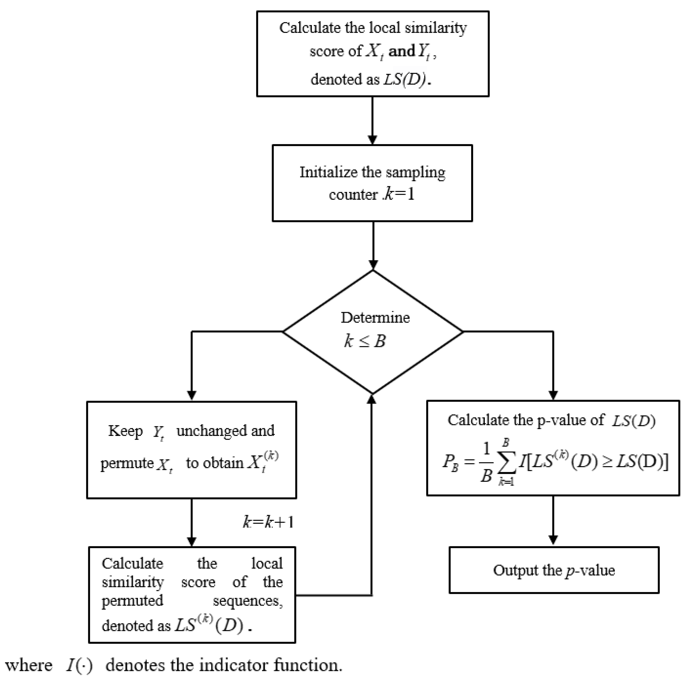
Figure 2.
Schematic Diagram of the Slider Selection Method.
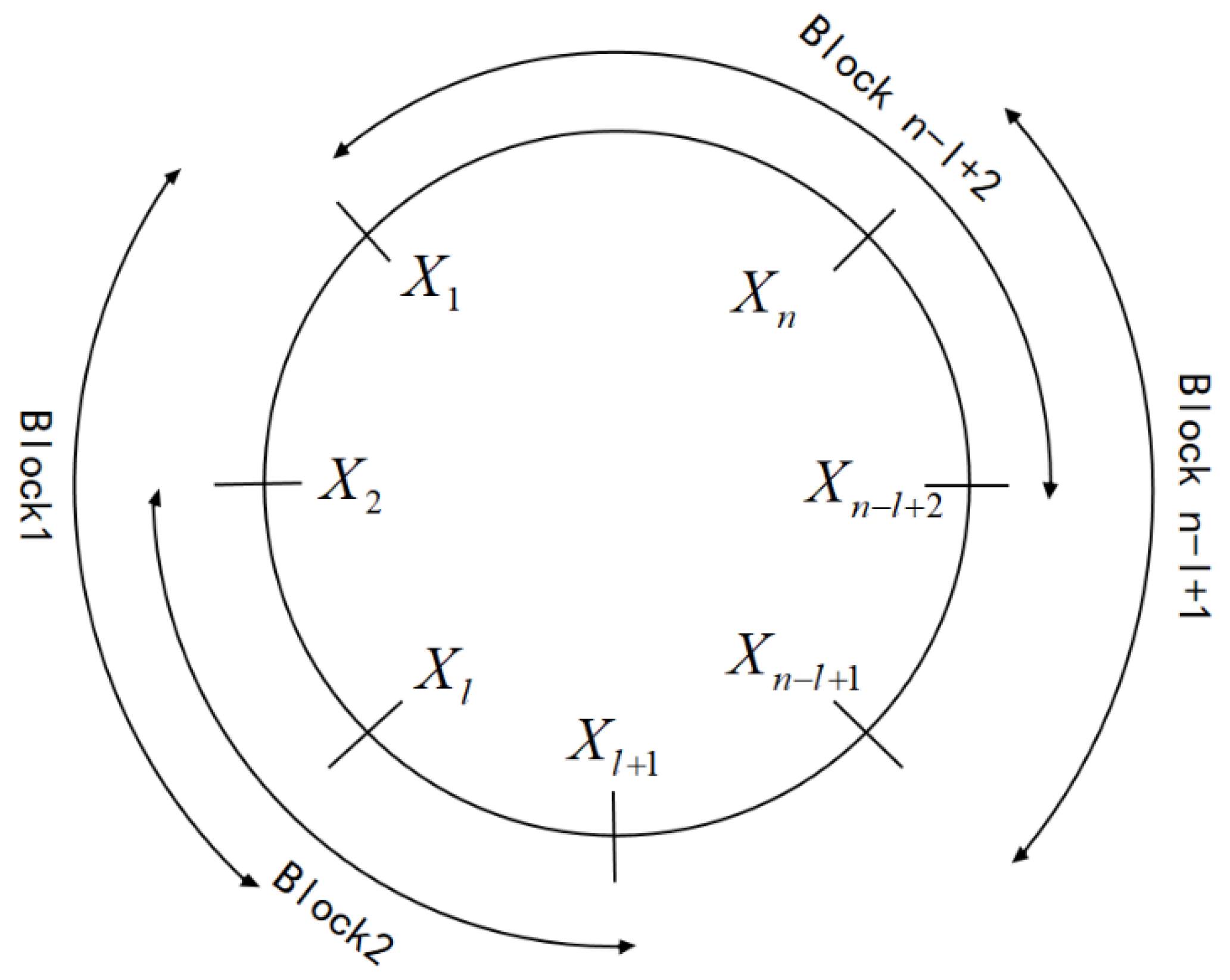
Figure 3.
Flowchart of the CMBBLSA computation.
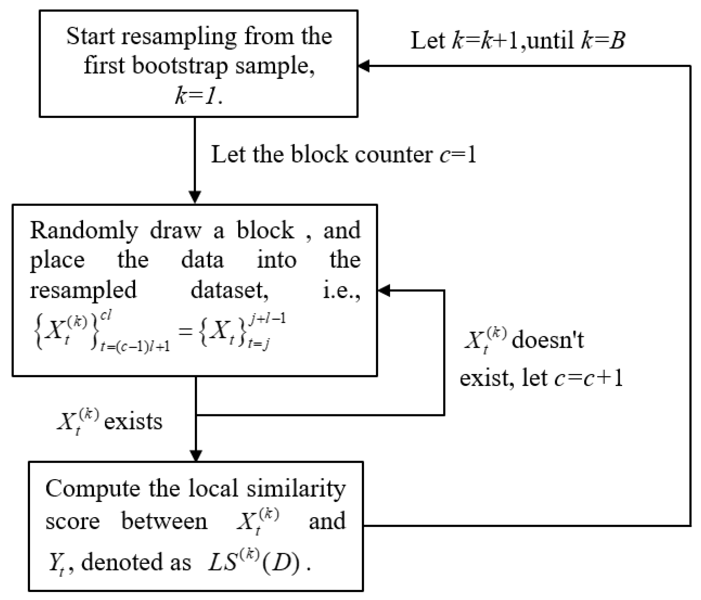
Figure 4.
Type I error rates at under different values of .
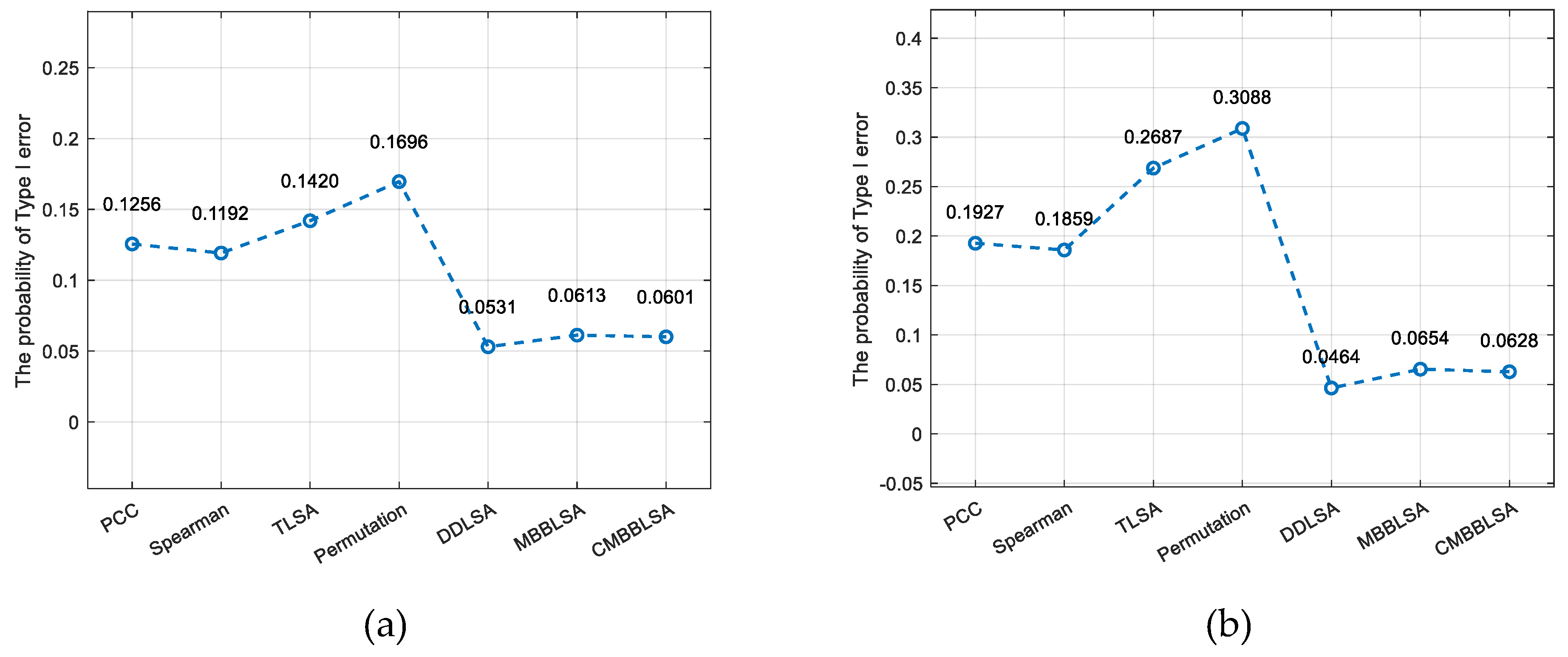
Figure 5.
Type I error rates at under different values of .
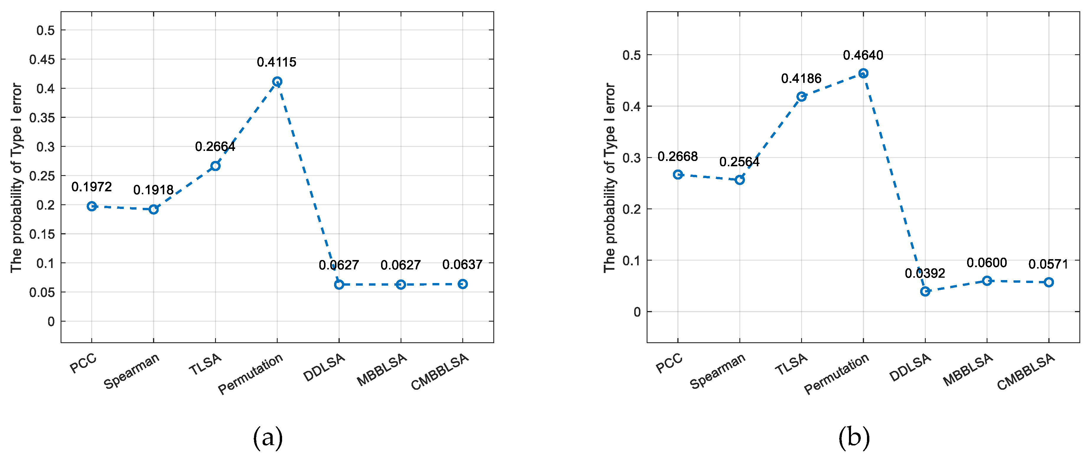
Figure 6.
Overlap of Significant Relationships by Different Methods.
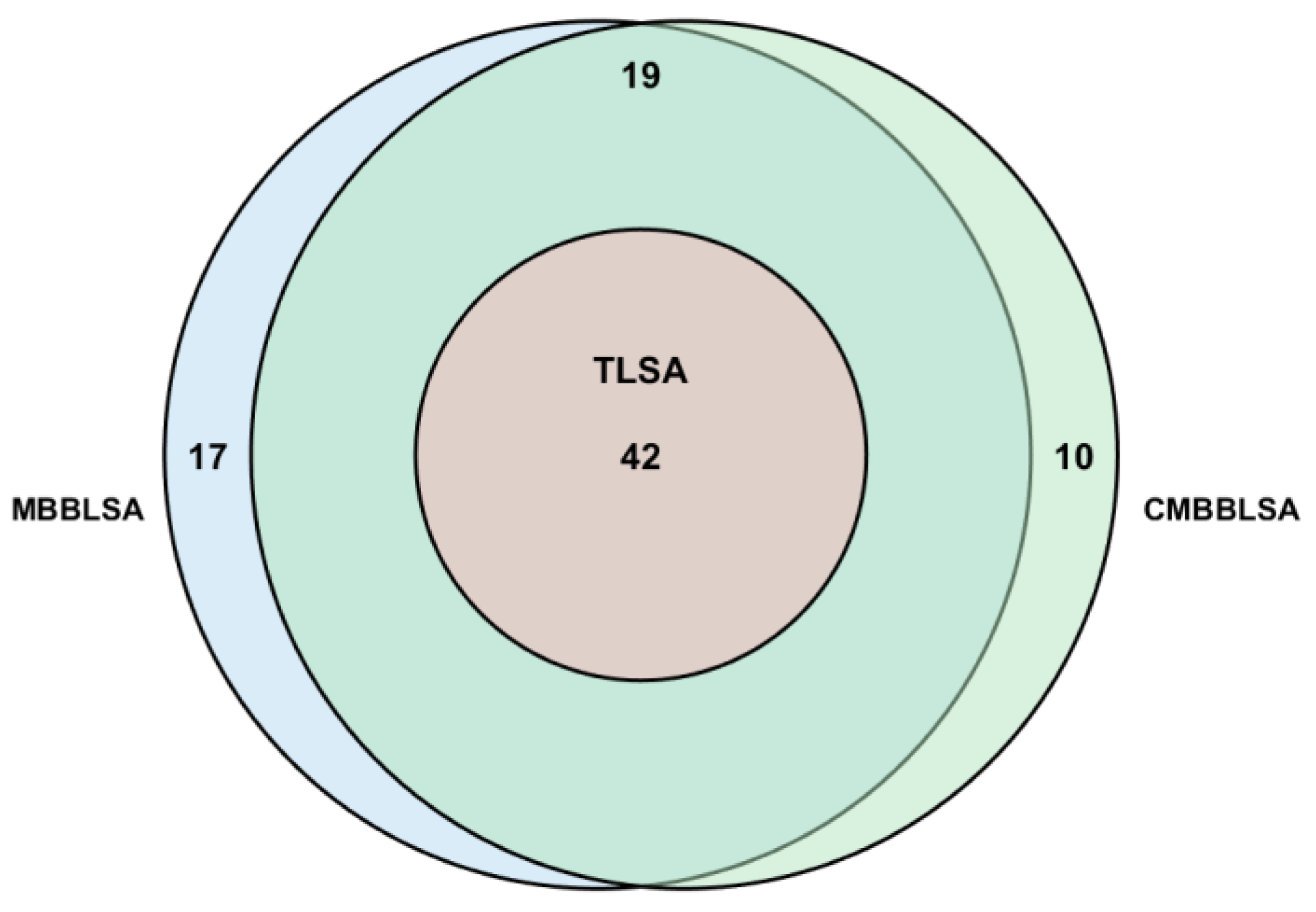
Figure 7.
Comparison Chart of Local Similarity Scores.
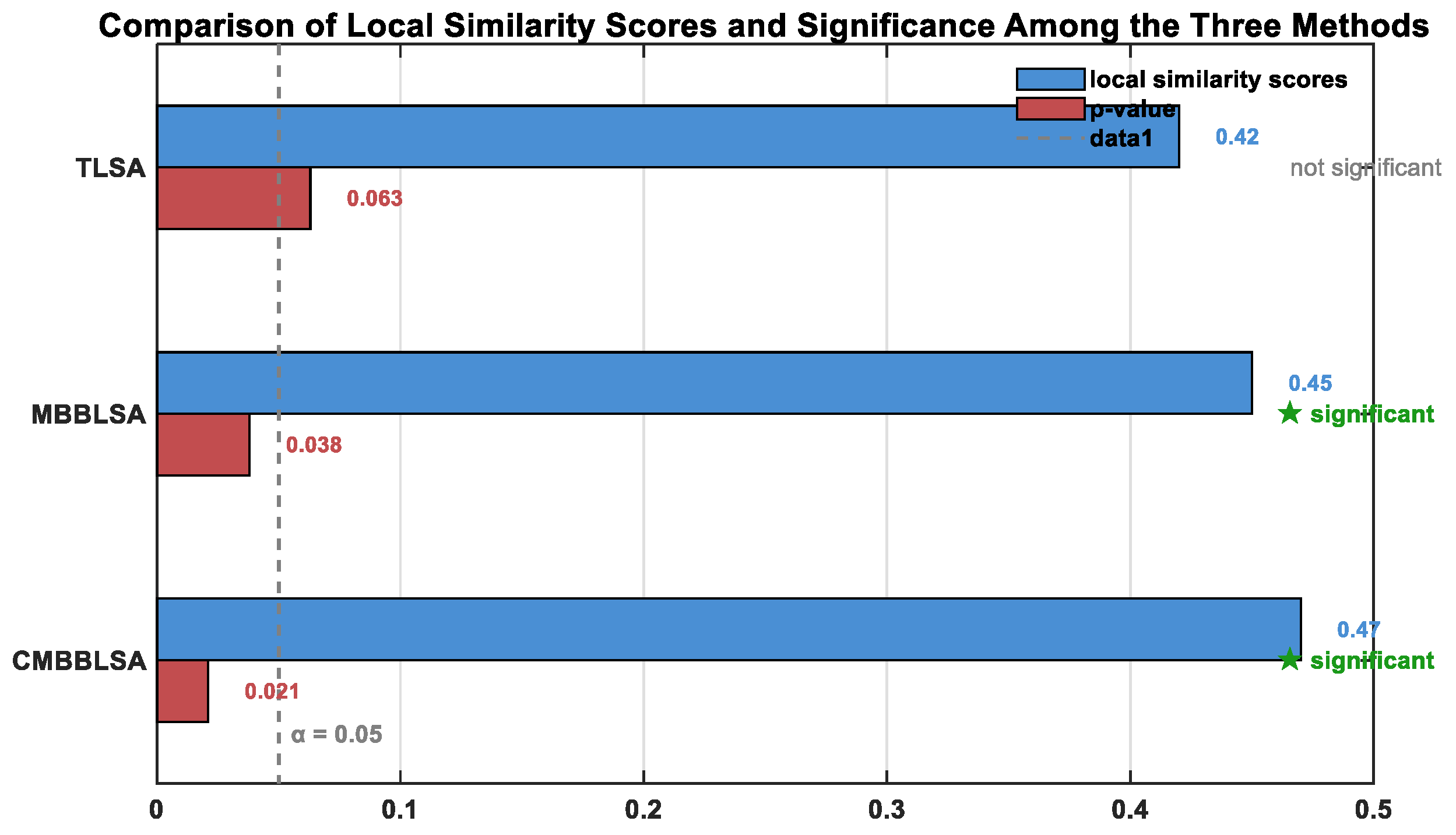
Table 1.
The probability of Type I error for different -values in the AR(1) model.
| n | PCC | Spearman | TLSA | Permutation | DDLSA | MBBLSA | CMBBLSA | |
| -0.5 -0.5 | 20 | 0.1063 | 0.1099 | 0.0407 | 0.1243 | 0.0198 | 0.0538 | 0.0499 |
| 40 | 0.1193 | 0.1136 | 0.0755 | 0.1408 | 0.0357 | 0.0575 | 0.0577 | |
| 60 | 0.1208 | 0.1156 | 0.0951 | 0.1502 | 0.0391 | 0.057 | 0.056 | |
| 80 | 0.1215 | 0.1198 | 0.104 | 0.157 | 0.039 | 0.0563 | 0.0539 | |
| 100 | 0.1245 | 0.1206 | 0.1182 | 0.1642 | 0.0432 | 0.0592 | 0.0547 | |
| 200 | 0.1275 | 0.1203 | 0.1376 | 0.1754 | 0.0461 | 0.0563 | 0.0548 | |
| 300 | 0.1328 | 0.1261 | 0.1527 | 0.1798 | 0.0497 | 0.0597 | 0.058 | |
| 0 0 | 20 | 0.0488 | 0.0469 | 0.0108 | 0.0496 | 0.0169 | 0.046 | 0.045 |
| 40 | 0.0531 | 0.0503 | 0.0225 | 0.0513 | 0.0264 | 0.0497 | 0.0502 | |
| 60 | 0.0489 | 0.0469 | 0.0242 | 0.0504 | 0.0287 | 0.0475 | 0.0486 | |
| 80 | 0.0464 | 0.0471 | 0.0264 | 0.0473 | 0.0279 | 0.0462 | 0.0463 | |
| 100 | 0.0499 | 0.049 | 0.0291 | 0.0513 | 0.0324 | 0.0491 | 0.05 | |
| 200 | 0.05 | 0.051 | 0.0346 | 0.0493 | 0.0363 | 0.0486 | 0.0496 | |
| 300 | 0.0477 | 0.0481 | 0.0373 | 0.0486 | 0.0383 | 0.0491 | 0.0496 | |
| 0.3 0.3 | 20 | 0.0645 | 0.0638 | 0.0161 | 0.0639 | 0.0227 | 0.0544 | 0.0532 |
| 40 | 0.0667 | 0.0659 | 0.0288 | 0.07 | 0.0286 | 0.0545 | 0.0534 | |
| 60 | 0.0697 | 0.0701 | 0.0395 | 0.0771 | 0.034 | 0.0575 | 0.057 | |
| 80 | 0.0742 | 0.0704 | 0.0473 | 0.0748 | 0.0417 | 0.0591 | 0.0565 | |
| 100 | 0.0716 | 0.0691 | 0.0486 | 0.0764 | 0.0401 | 0.0555 | 0.0544 | |
| 200 | 0.0722 | 0.0719 | 0.0618 | 0.0831 | 0.0476 | 0.0578 | 0.0563 | |
| 300 | 0.067 | 0.0704 | 0.061 | 0.0799 | 0.0445 | 0.0519 | 0.0502 | |
| 0.3 0.5 | 20 | 0.0795 | 0.0802 | 0.0198 | 0.077 | 0.022 | 0.0606 | 0.0587 |
| 40 | 0.0825 | 0.0837 | 0.0419 | 0.0888 | 0.0341 | 0.0613 | 0.0599 | |
| 60 | 0.0859 | 0.0848 | 0.0535 | 0.0931 | 0.0402 | 0.062 | 0.0583 | |
| 80 | 0.0878 | 0.0884 | 0.0622 | 0.1019 | 0.0417 | 0.0609 | 0.06 | |
| 100 | 0.0885 | 0.0873 | 0.07 | 0.1058 | 0.0457 | 0.0646 | 0.0621 | |
| 200 | 0.093 | 0.0888 | 0.0834 | 0.1098 | 0.0472 | 0.0605 | 0.0586 | |
| 300 | 0.0902 | 0.0859 | 0.0888 | 0.1115 | 0.0496 | 0.059 | 0.0575 | |
| 0.5 0.5 | 20 | 0.1046 | 0.1036 | 0.034 | 0.1079 | 0.0324 | 0.0724 | 0.0703 |
| 40 | 0.1157 | 0.1133 | 0.0668 | 0.1245 | 0.04 | 0.065 | 0.0646 | |
| 60 | 0.1175 | 0.1159 | 0.0851 | 0.1396 | 0.0413 | 0.0627 | 0.0626 | |
| 80 | 0.1223 | 0.1182 | 0.1009 | 0.1535 | 0.0467 | 0.0648 | 0.0644 | |
| 100 | 0.1151 | 0.1116 | 0.1033 | 0.1465 | 0.045 | 0.0622 | 0.0602 | |
| 200 | 0.1234 | 0.1192 | 0.1332 | 0.1675 | 0.0473 | 0.0602 | 0.0588 | |
| 300 | 0.1256 | 0.1192 | 0.142 | 0.1696 | 0.0531 | 0.0613 | 0.0601 | |
| 0.5 0.8 | 20 | 0.1484 | 0.1503 | 0.0559 | 0.1514 | 0.0359 | 0.0864 | 0.0847 |
| 40 | 0.1703 | 0.1731 | 0.1163 | 0.1985 | 0.045 | 0.0793 | 0.0712 | |
| 60 | 0.1859 | 0.1848 | 0.1529 | 0.224 | 0.0448 | 0.0763 | 0.0727 | |
| 80 | 0.1869 | 0.1814 | 0.1748 | 0.2388 | 0.0449 | 0.0742 | 0.0732 | |
| 100 | 0.1875 | 0.1837 | 0.1942 | 0.2584 | 0.0431 | 0.073 | 0.0712 | |
| 200 | 0.1939 | 0.1881 | 0.2442 | 0.2902 | 0.0511 | 0.0717 | 0.0703 | |
| 300 | 0.1927 | 0.1859 | 0.2687 | 0.3088 | 0.0464 | 0.0654 | 0.0628 |
Table 2.
The probability of Type I error for different ρ-values in the ARMA(1,1) model.
| n | PCC | Spearman | TLSA | Permutation | DDLSA | MBBLSA | CMBBLSA | |
| -0.5 -0.5 | 20 | 0.0482 | 0.0493 | 0.01 | 0.0475 | 0.0167 | 0.0455 | 0.0458 |
| 40 | 0.0472 | 0.0473 | 0.0202 | 0.0496 | 0.0226 | 0.0475 | 0.0478 | |
| 60 | 0.0516 | 0.0513 | 0.0251 | 0.0512 | 0.0293 | 0.0493 | 0.0502 | |
| 80 | 0.0489 | 0.0486 | 0.0268 | 0.0502 | 0.0301 | 0.0493 | 0.0498 | |
| 100 | 0.0504 | 0.05 | 0.0291 | 0.0484 | 0.0324 | 0.0479 | 0.0489 | |
| 200 | 0.0497 | 0.0523 | 0.0346 | 0.0512 | 0.0364 | 0.0516 | 0.0498 | |
| 300 | 0.0489 | 0.0503 | 0.0383 | 0.05 | 0.0391 | 0.0499 | 0.0502 | |
| 0 0 | 20 | 0.0858 | 0.0825 | 0.0237 | 0.0903 | 0.026 | 0.0658 | 0.0651 |
| 40 | 0.0823 | 0.0786 | 0.0396 | 0.0876 | 0.032 | 0.0576 | 0.0568 | |
| 60 | 0.0845 | 0.0799 | 0.0534 | 0.0899 | 0.0388 | 0.0567 | 0.0562 | |
| 80 | 0.085 | 0.0808 | 0.0602 | 0.0967 | 0.0439 | 0.059 | 0.0565 | |
| 100 | 0.0895 | 0.0841 | 0.0669 | 0.0997 | 0.0437 | 0.0596 | 0.0581 | |
| 200 | 0.0851 | 0.082 | 0.0749 | 0.1018 | 0.0453 | 0.0553 | 0.0547 | |
| 300 | 0.0857 | 0.0828 | 0.0841 | 0.105 | 0.046 | 0.0545 | 0.0533 | |
| 0.3 0.3 | 20 | 0.1274 | 0.1272 | 0.046 | 0.1361 | 0.0316 | 0.0745 | 0.0727 |
| 40 | 0.1316 | 0.1284 | 0.0866 | 0.1572 | 0.0383 | 0.0677 | 0.0675 | |
| 60 | 0.1357 | 0.1335 | 0.1066 | 0.1692 | 0.0373 | 0.0605 | 0.0605 | |
| 80 | 0.1455 | 0.1416 | 0.1267 | 0.1815 | 0.0427 | 0.067 | 0.065 | |
| 100 | 0.1391 | 0.1309 | 0.1348 | 0.1834 | 0.0397 | 0.0605 | 0.0586 | |
| 200 | 0.1398 | 0.1367 | 0.1558 | 0.1953 | 0.0444 | 0.0597 | 0.0595 | |
| 300 | 0.1433 | 0.1408 | 0.1786 | 0.212 | 0.0459 | 0.059 | 0.0588 | |
| 0.3 0.5 | 20 | 0.1454 | 0.1457 | 0.057 | 0.1543 | 0.0307 | 0.0756 | 0.0703 |
| 40 | 0.158 | 0.1534 | 0.1052 | 0.1851 | 0.0367 | 0.0678 | 0.0674 | |
| 60 | 0.1359 | 0.1523 | 0.133 | 0.1979 | 0.036 | 0.0636 | 0.0625 | |
| 80 | 0.1576 | 0.1561 | 0.1526 | 0.2086 | 0.0392 | 0.0657 | 0.0643 | |
| 100 | 0.166 | 0.1601 | 0.1665 | 0.2233 | 0.0423 | 0.0648 | 0.0628 | |
| 200 | 0.165 | 0.1561 | 0.1956 | 0.239 | 0.0406 | 0.0587 | 0.0573 | |
| 300 | 0.1637 | 0.1541 | 0.2178 | 0.2514 | 0.0427 | 0.0593 | 0.0569 | |
| 0.5 0.5 | 20 | 0.1786 | 0.1811 | 0.0802 | 0.1919 | 0.0364 | 0.0943 | 0.0812 |
| 40 | 0.1852 | 0.1848 | 0.1376 | 0.2222 | 0.0323 | 0.0693 | 0.0651 | |
| 60 | 0.1849 | 0.1841 | 0.1716 | 0.2511 | 0.0323 | 0.062 | 0.0598 | |
| 80 | 0.193 | 0.1856 | 0.1967 | 0.2708 | 0.0373 | 0.0602 | 0.0577 | |
| 100 | 0.1921 | 0.1869 | 0.2139 | 0.2808 | 0.0368 | 0.0598 | 0.0581 | |
| 200 | 0.1957 | 0.1901 | 0.2559 | 0.307 | 0.042 | 0.0567 | 0.0564 | |
| 300 | 0.1972 | 0.1918 | 0.2664 | 0.4115 | 0.0627 | 0.0627 | 0.0637 | |
| 0.5 0.8 | 20 | 0.225 | 0.2295 | 0.1102 | 0.2461 | 0.0282 | 0.1012 | 0.0868 |
| 40 | 0.2442 | 0.2437 | 0.1976 | 0.303 | 0.0295 | 0.0779 | 0.0736 | |
| 60 | 0.2514 | 0.2419 | 0.2443 | 0.3446 | 0.0278 | 0.0658 | 0.0654 | |
| 80 | 0.252 | 0.2543 | 0.2787 | 0.3634 | 0.0337 | 0.0698 | 0.07 | |
| 100 | 0.2544 | 0.2501 | 0.3063 | 0.3877 | 0.0316 | 0.0612 | 0.0606 | |
| 200 | 0.2647 | 0.2601 | 0.3826 | 0.4396 | 0.0402 | 0.0634 | 0.0622 | |
| 300 | 0.2668 | 0.2564 | 0.4186 | 0.464 | 0.0392 | 0.06 | 0.0571 |
Table 3.
Core Basic Information of the Dataset.
| Information Category | Concrete Content |
| Data Source | Intelligent Transportation System (ITS) of a first-tier city, monitoring station coordinates: 39°54′N, 116°23′E (downtown main road) |
| Collection Period | January 2023 – December 2023 (365 days total) |
| Sampling Interval | 5 minutes/interval, 8760 time points in total (continuous time series) |
| Core Variable Types | Traffic Flow Data, Speed Data, Environmental Factors |
| Final Selected Variables | 20 variables (12 traffic flow/speed variables + 8 environment-related variables) |
| Missing Value Handling Method | Piecewise Linear Interpolation |
Table 4.
Autocorrelation Test Results.
| Variable Type | Number of Variables |
Number of Significantly Autocorrelated Variables |
Proportion | Typical Variable Autocorrelation Coefficient (Lag 1) |
| Traffic Flow Data | 6 | 5 | 83.3% | Main Road A Morning Peak Flow: 0.68 (p=2.1×10⁻⁶) |
| Speed Data | 6 | 5 | 83.3% | Main Road B Evening Peak Speed: 0.52 (p=3.7×10⁻⁵) |
| Environmental Factors | 8 | 6 | 75.0% | Rainfall: 0.45 (p=1.2×10⁻⁴) |
| Total | 20 | 16 | 80.0% | -- |
Table 5.
Significantly Associated Relationships Count.
| Significance Level | TLSA | MBBLSA | CMBBLSA | False Positive Reduction Rate of CMBBLSA Compared to MBBLSA |
| =0.05 | 42 | 78 | 61 | 21.8% |
| =0.01 | 23 | 45 | 32 | 28.9% |
Disclaimer/Publisher’s Note: The statements, opinions and data contained in all publications are solely those of the individual author(s) and contributor(s) and not of MDPI and/or the editor(s). MDPI and/or the editor(s) disclaim responsibility for any injury to people or property resulting from any ideas, methods, instructions or products referred to in the content. |
© 2025 by the authors. Licensee MDPI, Basel, Switzerland. This article is an open access article distributed under the terms and conditions of the Creative Commons Attribution (CC BY) license (http://creativecommons.org/licenses/by/4.0/).
Copyright: This open access article is published under a Creative Commons CC BY 4.0 license, which permit the free download, distribution, and reuse, provided that the author and preprint are cited in any reuse.


