Preprint
Article

This version is not peer-reviewed.

Can Macroprudential Policy on Retail Banks Eliminate Bank Runs? Evidence from WAEMU’s Banking Sector

A peer-reviewed article of this preprint also exists.

Submitted:

08 December 2025

Posted:

11 December 2025

You are already at the latest version

Abstract

The aim of this paper is to determine a capital ratio for retail banks that can reduce the likelihood of bank runs in the WAEMU area. The study also compares the impact of imposing capital requirements on retail banks versus wholesale banks. The key finding are as follows: A capital ratio of 10 percent for retail banks is found to be sufficient to eliminate the probability of bank runs and mitigate interbank market frictions in the WAEMU area. Similarly, applying the same requirements to wholesale banks also eliminates the likelihood of bank runs. Implementing capital requirements on retail banks does not significantly affect interbank lending costs, whereas imposing the same requirements on wholesale banks leads to an increase in these costs. Consequently, regulating retail banks tends to shift assets towards wholesale banks, while regulating wholesale banks reallocates assets towards retail banks. The calculated capital ratio of 10 percent for retail banks maximizes welfare, surpassing the welfare achieved when the same requirements are imposed on wholesale banks.

Keywords: 
;  ;  ;  ;  ;  

1. Introduction

The global financial crisis of 2008 and the financial turmoil in March 2023 highlighted the importance of preventing bank failures, leading financial institutions such as the Bank for International Settlements and the Federal Reserve to tighten regulatory policies to ensure financial stability. Specifically, the minimum capital requirement regulation mandates that banks hold a minimum amount of capital relative to their total risk-adjusted assets.
In response to these concerns, the monetary and supervisory authorities of the West African Economic and Monetary Union (WAEMU) strengthened the regulatory framework through the Central Bank (BCEAO) and the Banking Commission. Following the global financial turbulence of 2023, the Council of Ministers of WAEMU decided to increase the minimum share capital of the Union's banks from XOF 10 to 20 billion, effective January 1, 2024. Additionally, a minimum capital ratio of 8.5% was set for the same year, which was met by 111 credit institutions, representing 86.0% of the institutions and accounting for 90.5% of total assets and 91.4% of risk-weighted assets in the banking system.
Numerous studies have shown the importance of macroprudential policies for financial stability. For example, Van den Heuvel (2008) found that a constant capital requirement of 10 percent can prevent banks from engaging in inefficient risk-taking. Recent studies have emphasized the need for higher capital requirements to discourage excessive risk-taking, with estimates ranging from 12 to 20 percent. These requirements not only reduce funding costs for banks but also enhance monitoring incentives and overall efficiency in banking activities. For instance, Collard et al. (2017) estimated that a Ramsey optimal capital requirement of 12 percent is sufficient to deter inefficient risk taking by banks. Begenau (2020) showed that an increased capital requirement from 9.25 percent to 12.38 percent for large banks, can decrease funding costs for banks and increase bank lending. A tighter capital requirement also enhances banks’ monitoring incentives, leading to greater efficiency in their activities. Another set of relevant papers analyzed the effects of capital requirements for financial stability (Christiano and Ikeda, 2016; Martinez-Miera and Suarez, 2014; Nguyen, 2014; Chari and Kehoe, 2016; Corbae and D’Erasmo, 2018; Gertler et al., 2016). Most of them indicated how imposing leverage constraints on banks can internalize credit externalities and decrease the social costs. In turn, Gertler et al. (2020) concluded that a capital requirement of 10 percent is sufficient to prevent the probability of bank runs. Nevertheless, their model makes unclear the distinction between commercial and shadow banks. By differentiating commercial (regulated) from shadow (unregulated) banks, Begenau and Landvoigt (2022) found that an optimal capital requirement about 20 percent for commercial banks makes both bank types safer. It directly strengthens commercial banks by reducing leverage and indirectly stabilizes shadow banks by influencing the valuation of intermediated assets.
Many of these studies have focused on US banks. In this paper, we aim to determine capital requirements for retail banks in the WAEMU region to prevent the probability of bank runs. By recalibrating a model economy with recent data from WAEMU banks, we also seek to compare the impact of implementing these capital requirements on retail banks versus wholesale banks. Our analysis is based on the model developed by Gertler, Kiyotaki, and Prestipino (2016), which focuses on banking and bank runs in the context of recent credit expansion and financial crises, distinguishing between retail and wholesale banks. This is an infinite horizon macroeconomic model with banking and bank runs developed in Gertler and Kiyotaki (2015).
The remainder of the paper is as follows: Section 2 describes the model. Section 3 explores numerical results. Section 4 debates discussion and Section 5 is about conclusion.

2. Framework

2.1. Key Features

The model features four types of agents: households, retail and wholesale banks and a regulator setting a prudential policy. There are two goods, a nondurable goods and a durable asset, which is capital. There is no capital’s depreciation, and the total supply of capital stock is normalized to unity. Wholesale and retail banks acquire capital through borrowed funds and their own equity. Households lend to banks and hold capital directly.
K t w + K t r + K t h = K ¯ = 1 ,       1
where K t w , K t r , and K t h are the total capital held by wholesale and retail bankers, and households respectively.
Expenditure in terms of goods at time t reflects the management cost of screening and monitoring investment projects. In the case of retail banks, the management costs might also reflect various regulatory constraints. We assume this management cost is increasing and convex in the total amount of capital, as given by the following quadratic formulation:
F j K t j = α j 2 K t j 2 .       B . 3
where type j = w , r , and h represents wholesale banks, retail banks and households, respectively. The marginal cost from providing the management service is denoted by:
f t j = F j ' K t j = α j K t j . B . 4
In addition, we assume the management cost is zero for wholesale banks and highest for households (holding constant the level of capital):
Assumption 1:  α w = 0 < α r < α h .
This assumption implies that wholesale bankers have an advantage over the other agents in managing capital. Retails banks in turn have a comparative advantage over households.

2.2. Households

Households consume and save either by lending funds to bankers or by holding capital directly in the competitive market. They may deposit funds in either retail or wholesale banks. In addition to the returns on portfolio investment, every period each household receives an endowment goods, Z t W h , that varies proportionately with the aggregate productivity shock Z t .
Deposits held in a bank from t to t + 1 are one period bonds that promise to pay the noncontingent gross rate of return R ¯ t + 1 in the absence of a run by depositors. In case of a deposit run, depositors only receive a fraction x t + 1 r of the promised return, where x t + 1 r is the total liquidation value of retail banks assets per unit of promised deposit obligations.
In consequence, the household’s return on deposits, R t + 1 is expressed as follows:
R t + 1 = R ¯ t + 1   i f   n o   d e p o s i t   r u n x t + 1 r R ¯ t + 1   i f   d e p o s i t   r u n   o c c u r s     2
where 0 x t r < 1 .
If a deposit run occurs all depositors receive the same pro rata share of liquidated assets.
Household utility U t is given by:
U t = E t i = 0 β i l n C t + i h
where C t h is the household’s consumption and 0 < β < 1 .
The household chooses consumption, bank deposits D t and direct capital holdings K t h to maximize expected utility subject to the budget constraint:
C t h + D t + Q t K t h + F h K t h = Z t W h + R t 1 D t 1 + Z t + Q t K t 1 h + f t r K t r F r K t r . 3
Consumption, saving, and management costs are financed by the endowment W h , the returns on savings, and the profits from providing management services to retail bankers. Q t is the market price of capital.
The household chooses consumption and saving with the expectation that the realized return on deposits, R t + i equals the promised return R ¯ t + 1 with certainty, and that asset prices Q t + i are those at which capital is traded when no bank run happens. (See Appendix B for the first-order conditions).
Moreover, the innovation shock Z t follows an A R 1 model:
Z t = ρ z Z t 1 + σ ε t + 1 . 4
where ρ z is the autoregressive parameter, σ the perturbation term and ε t is n.i.i.d process with variance σ ε 2 .

2.3. Banks

There are two types of bankers: retail and wholesale. Each type manages a financial intermediary. Banks fund capital investment, which refers to nonfinancial loans by issuing deposits to households, borrowing from other banks in an interbank market and using their own equity. Banks can also lend in the interbank market.
Bankers may be vulnerable to runs in the interbank market. In this case, creditor banks suddenly decide to not rollover interbank loans. In the event of an interbank run, the creditor banks receive a fraction x t + 1 w of the promised return on the interbank credit, where x t + 1 w is the total liquidation value of debtor bank assets per unit of debt obligations. Thus, the creditor bank’s return on interbank loans, R b t + 1 is as follows:
R b t + 1 = R ¯ b t + 1   i f   n o   i n t e r b a n k   r u n x t + 1 w R ¯ b t + 1   i f   i n t e r b a n k   r u n   o c c u r s , 5
where 0 x t w < 1 . If an interbank run occurs, all creditor banks receive the same pro rata share of liquidated assets.
Due to financial market frictions, bankers may be constrained in their ability to raise external funds. To the extent they may be constrained, they will attempt to save their way out of the financing constraint by accumulating retained earnings in order to move towards 100% equity financing. To limit this possibility, we assume that bankers have a finite expected lifetime: specifically, each banker of type j ( = w ,   r ) has an i . i . d . probability σ j of surviving until the next period and a probability 1 σ j of exiting.
Every period new bankers of type j enter with an endowment W j that is received only in the first period of life. This initial endowment may be thought of as the start up equity for the new banker. The number of entering bankers equals the number who exit, keeping the total constant.
To encourage the use of wholesale funding markets along with retail markets, we assume that the banker’s ability to divert funds depends on both the sources and uses of funds. The banker can divert the fraction θ of nonfinancial loans financed by retained earnings or funds raised from households, where 0 < θ < 1 . On the other hand, he/she can divert only the fraction θ ω of nonfinancial loans financed by interbank borrowing, where 0 < ω < 1 . Here, bankers lending in the wholesale market are more effective at monitoring the banks to which they lend than are households that supply deposits in the retail market.
For bankers that lend to other banks, we suppose that it is more difficult to divert interbank loans than nonfinancial loans. Specifically, we suppose that a banker can divert only a fraction θ γ of its loans to other banks, where 0 < γ < 1 . ω and γ are the parameters that govern the moral hazard problem in the interbank market.
The banker’s decision at t reduces to comparing the franchise value of the bank V t j , which measures the present discounted value of future payouts from operating honestly, with the gain from diverting funds. In this regard, rational lenders will not supply funds to the banker if he has an incentive to cheat. Thus, any financial arrangement between the bank and its lenders must satisfy the following set of incentive constraints:
V t j θ Q + f j K t j b t j + ω B t j , if B t j > 0 (net borrower)
V t j θ Q t + f t j K t j + γ K t j , if B t j < 0 (net lender), 6
Overall, there are two basic factors that govern the existence and relative size of the interbank market. First, the cost advantage that wholesale banks have in managing nonfinancial loans as in Assumption 1. Second, the size of the parameters ω and γ which govern the comparative advantage that retail banks have over households in lending to wholesale banks, as shown by Assumption 2.
Assumption 2:  ω + γ > 1 .
This implies that ω and γ can be sufficiently small to permit an empirically reasonable relative amount of interbank lending.
The banker’s evolution of net worth is thus:
N t + 1 j = R k t + 1 j Q t + f t j K t j R t + 1 D t j R b t + 1 B t j , 7
where R k t + 1 j is the rate of return on nonfinancial loans, given by:
R k t + 1 j = Q t + 1 + Z t + 1 Q t + f t j .     8
The stochastic discount factor Ω t + 1 j , which the bankers use to value N t + 1 j is a probability weighted average of the discounted marginal values of net worth to exiting and continuing bankers at t + 1 .
Ω t + 1 j = β 1 σ j + σ j V t + 1 j N t + 1 j , 9
where V t + 1 j / N t + 1 j is the Tobin’s Q ratio.
The banker’s optimization problem then is to choose K t j , D t j , B t j   each period to maximize the franchise value subject to the incentive constraint and the balance sheet constraints and E q . 9 .

2.3.1. Wholesale Banks

Generally, wholesale banks may raise funds either from other banks or from households. Especially, the model focuses on wholesale funding markets equilibrium where the conditions for the Lemma 1 are satisfied:
Lemma 1:  D t w = 0 , B t w > 0 and the incentive constraint is binding if and only if
0 < ω E t Ω t + 1 w R k t + 1 w R t + 1 < E t Ω t + 1 w R k t + 1 w R b t + 1 < θ ω
Given Lemma 1 the evolution of bank net worth is:
N t + 1 w = R k t + 1 w R b t + 1 ϕ t w + R b t + 1 N t w , ( 10 )
where the multiple leverage ratio ϕ t w is given by:
ϕ t w Q t K t w N t w . ( 11 )
In turn, the wholesale banks optimization problem to choosing the leverage multiple to solve:
V t w = max ϕ t w E t Ω t + 1 w R k t + 1 w R b t + 1 ϕ t w + R b t + 1 N t w , ( 12 )
subject to the incentive constraint
θ ω ϕ t w + 1 ω N t w V t w . 13
Given the incentive constraint is binding under Lemma 1, the objective combines with the binding incentive constraint to obtain the following solution for ϕ t w :
ϕ t w = E t Ω t + 1 w R b t + 1 θ 1 ω θ ω E t Ω t + 1 w R k t + 1 w R b t + 1 . 14
ϕ t w is increasing in E t Ω t + 1 w R k t + 1 w and decreasing in E t Ω t + 1 w R b t + 1 . Intuitively, the franchise value V t w increases when returns on assets are higher and decreases when the cost of funding asset purchases rises as indicated by E q . 12 . Increases in V t w loosen the incentive constraint, making lenders will, to supply more credit.
Likewise, ϕ t w is a decreasing function of both θ , the diversion rate on nonfinancial loans funded by net worth, and ω , the parameter that controls the relative ease of diverting nonfinancial loans funded by interbank borrowing relative to those funded by the other means: increases in either parameter tighten the incentive constraint, inducing lenders to reduce the amount of credit they supply.
Lastly, from E q . 12 , an expression of the franchise value per unit of net worth or the shadow value of wholesale bank net worth, that we call φ t w is set as:
φ t w = V t w N t w = E t Ω t + 1 w R k t + 1 w R b t + 1 ϕ t w + R b t + 1 > 1 15 ,
where ϕ t w is given by E q . 14 . The shadow value φ t w is greater than 1 since extra net worth enables the bank to borrow more and invest in assets earning an excess return.

2.3.2. Retail Banks

As with wholesale banks, the model opts for a parametrization where the incentive constraint binds and narrows to the case where retail banks are holding both nonfinancial and interbank loans. Particularly, the model considers a parametrization where in equilibrium Lemma 2 is satisfied:
Lemma 2:  B t r < 0 ,   K t r > 0 and the incentive constraint is binding if and only if
0 < E t Ω t + 1 r R k t + 1 r R t + 1 = 1 γ E t Ω t + 1 r R b t + 1 R t + 1 < 0 .
For the retail bank to be indifferent between holding nonfinancial loans, the rate on interbank loans R b t + 1 must be below the rate earned on nonfinancial loans R k t + 1 r in a way that satisfies the conditions for the lemma. Intuitively, the advantage for the retail bank to making an interbank loan is that households are willing to lend more to the bank per unit of net worth than for a nonfinancial loan. Therefore, to make the retail bank indifferent, R b t + 1 must lie below R k t + 1 r .
Let ϕ t r be a retail bank’s effective leverage multiple, namely the ratio of assets to net worth, where assets are weighted by the relative ease of diversion:
ϕ t r Q t + f t r K t r + γ B t r N t r . 16
The weight γ on B t r is the ratio of how much a retail banker can divert from interbank loans relative to nonfinancial loans.
Given the restrictions implied by lemma 2, the same procedure is used as in the case of wholesale bankers to express the retail banker’s optimization problem as choosing ϕ t r to solve:
V t r = max ϕ t r E t Ω t + 1 r R k t + 1 r R t + 1 ϕ t r + R t + 1 N t r , 17
subject to
θ ϕ t r N t r V t r .
Given Lemma 2, imposing that incentive constraint binds, which implies:
ϕ t r = E t Ω t + 1 r R t + 1 θ E t Ω t + 1 r R k t + 1 r R t + 1 . 18
As with the leverage multiple for wholesale bankers, ϕ t r is increasing in expected asset returns on the bank’s portfolio and decreasing in the diversion parameter.
At the end, from E q . 17 an expression for the franchise value per unit of net worth is as follows:
φ t r = V t r N t r = E t Ω t + 1 r R k t + 1 r R t + 1 ϕ t r + R t + 1 . 19
As with wholesale banks, the shadow value of a unit of net worth exceeds unity and depends only on aggregate variables.

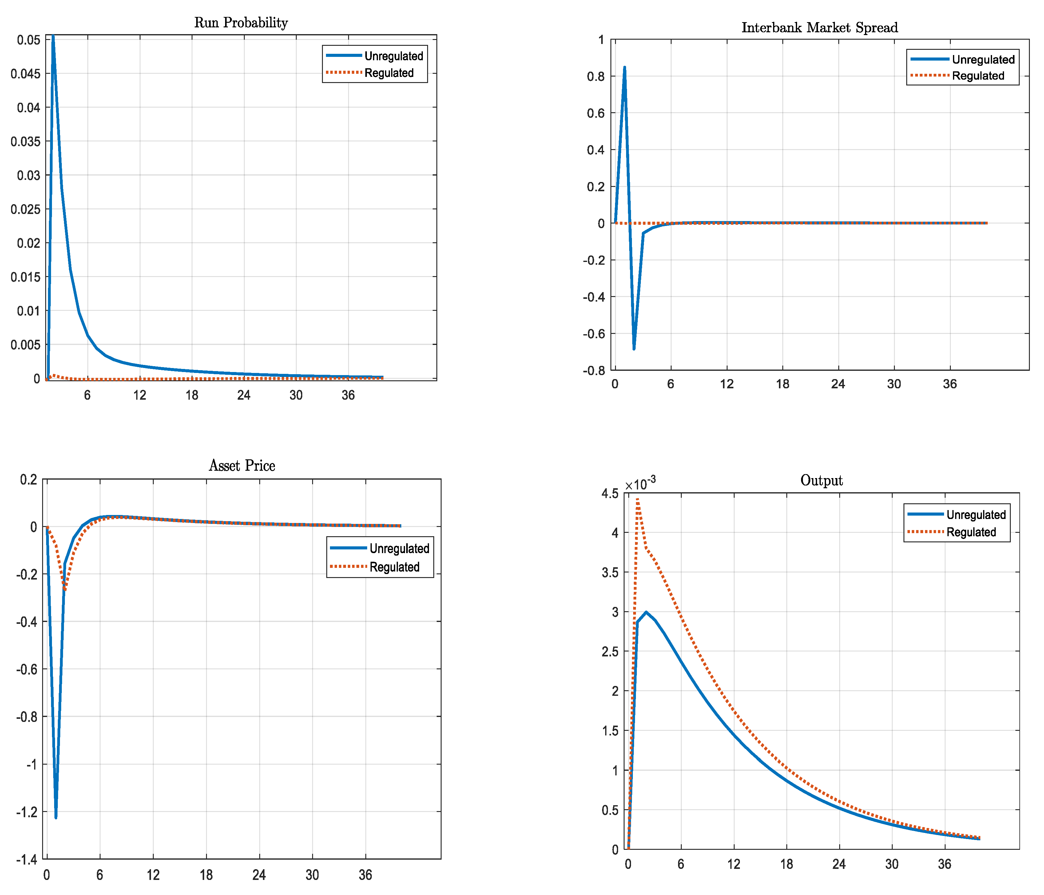
2.3.3. Recessions and Runs

This section deals with the scenario where the economy goes into recession, which involves a drop in Z t , making a bank run equilibrium possible. In this instance, the run variable is defined as:
R u n t w = 1 x t w , 20
where x t w is the recovery rate on wholesale debt. Hence, for a run to exist the run variable must be positive or the recovery rate is less than unity, i.e., (see Appendix C for the proof)
x t w = Z t + Q t * K t 1 w R b t B t 1 = R k t w * R b t ϕ t 1 w ϕ t 1 w 1 < 1 . , 21
where R k t w * is the return on bank assets conditional on a run at t   R k t w * Z t + Q t * Q t 1 , and Q t * the liquation price expressed as below:
Q t * = E t i = 1 Λ t , t + i Z t + i α h K t + i h α h K t h . 22
According to Gertler and Kiyotaki (2015) at each time t , the probability of transitioning to a state where a run on wholesale banks occurs, is given by a reduced form decreasing function of the expected recovery rate E t x t + 1 w as follows:
p t = 1 E t x t + 1 w δ . 23
This formulation allows to capture the idea that as wholesale balance sheet positions weaken, the likelihood of a run increases. In the numerical simulations, δ is set to δ = 0.5 .

2.4. Macroprudential Policy

Banks may encounter a moral hazard problem, where they must decide to operate honestly or to divert assets for personal use, thus the latter affecting their ability to raise funds. If they choose to divert, the consequence for the banker is that the creditors can push the financial intermediary into bankruptcy at the start of the subsequent period. As a consequence of this, bank runs can arise from either a deposit run or the inability of banks to meet their obligations. To rule out the probability of bank runs, the financial regulator imposes capital requirements on banks. Specifically, banks are subject to Basel-III-type capital requirements. Under the Basel III accords, banks are required to hold a set proportion of their risk-weighted assets in equity.
The time-varying capital requirement for retail banks is then:
k t = N t r Q t K t r θ φ t r ,     ( 24 )
Equation 24 shows that an increase in the shadow value of net worth φ t r , decreases the bank capital requirement, making the financial sector more fragile with possible bank runs. The capital requirement is also increasing in the diversion rate θ . In response to shocks that increase banks’ risk-taking, the regulator should raise the level of capital requirements.
Appendix A depicts the market clearing conditions

3. Numerical Results

This section presents the parameters values used to solve the model and turn to numerical findings resulting from the integration of capital requirements. The model is solved nonlinearly, using perturbation methods. A good idea to have a nonstationary model is that we can control the level of technology. Since Maih’s perturbation is also suitable for regime-switching, constant-parameters DSGE and RBC models, then the solution of the model is based on this type of perturbation. All numerical results are conducted using RISE software.

3.1. Parameters Values

We calibrate the model to 2023 WAEMU’s banks data. This period is marked not only by a weak banking regulation and persistent inflationary tensions observed in 2022, but also by the financial turmoil in March 2023, mainly due to incentive measures taken in favor of WAEMU’s economies and across the world, following the COVID-19’s crisis. Indeed, the households’ discount factor β is set at the conventional value β = 0.99 . The endowment is equal to W h = 0.006 , W r = 0.0008 , and W w = 0.0008 , for households, retail and wholesale banks respectively, while the persistence parameter of the AR(1) process ρ z equals 0.90 , as in Gertler et al. (2016) and a standard error σ z = 0.01 for its innovations. Based on financial soundness indicators from IMF (2023), the average funding cost and interest margins were around 2% and 5.1% respectively, indicating that WAEMU’s retail banks maintained a net interest margin of roughly 3.1% in 2023. This leads to the managerial costs of intermediating capital for households and retail bankers α h and α r for the spread between the deposit rate and retail bankers’ returns on loans as well as the difference between wholesale bankers and retail bankers’ returns on loans to be respectively 0.2% and 0.3% annually in steady state.1 The estimated average on the divertible proportion of assets in 2023 for retail and wholesale banks are based on triangulated data and from reports, such as BCEAO’s annual report (2023) and its statistical database, banking commission report, and IMF-WAEMU FSAP2 reports. This leads to θ = 0.30 and ω = 0.55 . This difference reflects the functional specialization since wholesale banks are designed for interbank and capital market operations, whereas retail banks for deposit-taking and households lending. From the same data sources, the fraction of divertible interbank loans γ is set to 0.70, leading to an annualized steady state spread between deposit and interbank rates of 0.14%. As of 2023, the survival probability of retail banks in the WAEMU area is generally high compared to wholesale banks, but variable, depending on the country and the size/type of the bank. By using countries specific banks data from mainly Banking Commission Annual Report (2023), and IMF Financial Stability Review-WAEMU (2023), we compute the average estimated 1-year survival probability for retail and wholesale banks to σ r = 0.96 and σ w = 0.89 . Then, Table 1 displays all parameters of the model.

3.2. Long Run Implications of Capital Requirements

This section discusses the model properties under macroprudential regulation, further exhibits the impulse response functions.

3.2.1. Model Properties Under Capital Requirements

Table 2 presents the key variables before and after the implementation of the capital requirement (old regime vs. new regime) along with the corresponding percentage changes. In Block 1, the second column shows the steady-state values under capital requirements for retail banks, while in Block 2, the second column displays the steady-state values for wholesale banks. The third column in each block indicates the percentage change between the new and old regimes. For our calibration, we find that the steady-state value of k t * is 10% for retail banks.
Households prefer the new regime in Block 1, leading to a significant increase in consumption (+9.09% compared to +8.82% in Block 2). This higher consumption level results in a 1.27% reduction in the equilibrium level of deposits (compared to a 12.05% decrease in Block 2).
Maintaining the interbank lending rate stable under the new regime allows retail banks to sustain credit supply in Block 1. This stability leads to an unchanged allocation of assets between both types of banks, keeping banks' return on assets consistent from the old to the new regime. Conversely, a 0.05% increase in the interbank rate in Block 2 makes lending less profitable for retail banks, prompting a 53.13% decrease in credit provision and a shift in asset allocation. This reduction increases retail banks' capital by over 100% and decreases wholesale banks' capital by 45.90%, resulting in a 0.07% increase in retail banks' return on assets and a 0.13% decrease in wholesale banks' return on assets.
The policy induced rise in asset prices by 6.14% in Block 1 and 1.96% in Block 2 has general equilibrium effects on banks' balance sheets, leading to improved capitalization and increased net worth. In Block 1, net worth increases by 11.87% for wholesale banks and 17.41% for retail banks, while in Block 2, the increases are 0.90% for wholesale banks and 4.21% for retail banks, reducing leverage in both banking sectors. Consequently, output increases by approximately 11.45% in Block 1 and 6.43% in Block 2.
We follow Begenau and Landvoigt (2022) in calculating the induced welfare for a capital requirement level of k * = 10 % , first implemented on retail banks and then on wholesale banks, as shown in Table 2. We simulate the model over multiple periods to obtain moments of the simulated variables. Welfare is measured as the percentage change in the mean and standard deviation of the household value function relative to the unregulated economy in each scenario, as presented in Table 3. Cases 1&3 in column 2 show the unconditional moments of key variables in the unregulated economy, while Cases 2&4 in column 3 represent their counterparts in the regulated economy. The results indicate that imposing a 10% capital ratio on retail banks (Case 2) leads to greater welfare gains (10%) and lower volatility (-17.46%) compared to applying the same requirements to wholesale banks (Case 4), where welfare improves by 7.38% and volatility increases by 16.67%.

3.2.2. Impulse Responses Under Capital Requirements ( k * = 10 % )

This section examines the effects of applying capital requirements to retail banks compared to the effects of implementing the same requirements on wholesale banks. The derived capital ratio for retail banks is, k * = 10 % at the steady-state.
3.2.2.1. Effects of Implementing Capital Requirements ( k * = 10 % ) on Retail Banks
Figure 1 displays the impulse response functions of the economy to a negative 6% shock to productivity with and without anticipated bank runs, with and without macroprudential regulation. The solid line represents the unregulated economy, while the dotted line represents the economy where the regulator enforces capital requirements on retail banks. The results show that capital requirements for retail banks eliminate the probability of a bank run by reducing interbank market frictions and lowering banks' leverage. In contrast, in the unregulated economy, the probability of a bank run remains high for several years, reaching about 5% in the first year of the recession, leading to increased leverage and exacerbating interbank market volatility. Furthermore, the policy has a significant stimulative effect on asset prices, with an increase of approximately 6.14% within the first two years of the recession. This rise in asset prices boosts banks' net worth, impacting output, which increases by 11.45% compared to the unregulated economy. Additionally, the regulation leads to a reallocation of assets towards wholesale banks, resulting in losses on retail banks' capital investments in favor of wholesale banks.
3.2.2.2. Effects of Implementing Capital Requirements ( k * = 10 % ) on Wholesale Banks
Figure 2 displays impulse response functions of the economy with anticipated bank runs to a negative 6% shock to productivity with and without macroprudential regulation. The solid line represents the unregulated economy, while the dotted line illustrates the economy under which a capital ratio of 10% is imposed by the regulator on wholesale banks. The results suggest that applying the same capital ratio to wholesale banks as retail banks eliminates the probability of a bank run and reduces financial frictions in the interbank market, while also controlling banks' leverage. However, over time, the probability of a bank run remains high, exceeding 30%, indicating persistent instability in the interbank market in the unregulated economy. Under the regulation, asset prices experience a significant increase of approximately 1.96% within the first two years of the recession, mitigating the drop in output by around 6.43%, which is lower than in the regulated economy shown in Figure 1. In contrast to Figure 1, implementing the same capital ratio on wholesale banks leads to a reallocation of assets towards retail banks, resulting in losses on wholesale banks' capital investments due to higher funding costs in the regulated economy (see Table 2).

4. Discussion

We establish a capital ratio for retail banks to mitigate the likehood of bank runs in the WAEMU area. We also compare the impact of imposing this capital requirement on retail banks versus wholesale banks. Our analysis shows that a 10 percent capital ratio effectively reduces the likelihood of bank runs, minimizes interbank market frictions, and limits banks' leverage. This indicates that even a modest capital requirement of 10 percent can enhance financial system resilience and discourage risky behavior by banks in the WAEMU area. Previous studies using US data have also demonstrated that a 10 percent risk-based capital ratio is sufficient to prevent bank runs (Van den Heuvel, 2008; Gertler et al., 2020). Implementing the policy on retail banks leads to higher asset prices, improved capitalization, and a more significant impact on output compared to applying the policy to wholesale banks (refer to Table 2 and Figures 1 & 2). Additionally, imposing macroprudential regulations on retail banks results in a slight shift of assets towards wholesale banks. This policy maintains the interbank rate at its current level in the unregulated economy, encouraging retail banks to maintain credit supply and enabling wholesale banks to protect their capital investments. Conversely, applying the same policy to wholesale banks redirects assets towards retail banks by increasing the interbank rate relative to its level in the unregulated economy, making lending less profitable for retail banks and prompting them to reduce credit provision. Consequently, wholesale banks decrease their capital investments in favor of retail banks (refer to Table 2, Figures 1 & 2). The study suggests that imposing the same level of capital requirements on retail and wholesale banks influences the asset allocation between the two types of banks. Research has shown that tightening capital requirements for commercial banks from the current 10% level prompts households to shift from commercial bank liquidity to shadow bank liquidity (Begenau and Landvoigt, 2022). Furthermore, the analysis reveals that implementing capital requirements for retail banks leads to higher consumption and welfare compared to applying the same requirements to wholesale banks (refer to Table 3). This indicates that implementing capital requirements on retail banks is more beneficial for welfare than imposing them on wholesale banks. Studies using US commercial banks data have consistently shown that varying levels of capital requirements can maximize welfare (Begenau and Landvoigt, 2022; Begenau, 2020; Collard et al., 2017; Van den Heuvel, 2008).

5. Conclusion

This study focuses on deriving capital requirements for retail banks in the WAEMU area to prevent bank failures. Likewise, it compares the effects of implementing capital requirements on retail banks to wholesale banks. The findings show that setting a capital ratio for retail banks can prevent bank runs and mitigate recessionary effects. Similarly, applying the same capital ratio to wholesale banks produces similar results. The allocation of assets between retail and wholesale banks is influenced by the capital ratio for retail banks. Future research could explore setting different risk-based capital ratios for wholesale banks compared to retail banks in the WAEMU area.

Appendix A. Aggregate

Once the conditions in Lemma 1 and 2 are satisfied, the following aggregation is made across banks to obtain relations between total assets and net worth for both the wholesale and retail banking sectors. Let Q t K t w and Q t K t r be total nonfinancial loans held by wholesale and retail banks, D t be retail bank deposits, B t be total interbank debt, and N t w and N t r total net worth in each respective banking sector.
We get:
Q t K t w = ϕ t w N t w , A . 1
Q t + f t r K t r + γ B t = ϕ t r N t r , A . 2
with
Q t K t w = N t w + B t , A . 3
Q t + f t r K t r + B t = D t r + N t r , A . 4
and
E t Ω t + 1 r R k t + 1 r R t + 1 = 1 γ E t Ω t + 1 r R b t + 1 R t + 1 , A . 5
A . 5 underwrites that the retail bank is indifferent at the margin between holding nonfinancial loans or interbank loans (Lemma 2).
Summing across both surviving and entering bankers produces the next expression for the evolution of N t :
N t w = σ w R k t w R b t ϕ t 1 w + R b t N t 1 w + W w , A . 6
N t r = σ r R k t r R t ϕ t 1 r + R t N t 1 r + W r + σ r R b t R t γ R k t r R t B t 1 , A . 7
where W j = 1 σ j w j is the total endowment of entering bankers. The first term is the accumulated net worth of bankers that operated at t 1 and survived to t , which is equal to the survival rate σ j times the net earnings on bank assets.
Total consumption of bankers equals the sum of the net worth of exiting bankers in each sector:
C t b = 1 σ w N t w W w σ w + 1 σ r N t r W r σ r , A . 8
Total gross output Y ¯ t is the sum of output from capital, household endowment Z t W h and bank endowment W r and W w :
Y ¯ t = Z t + Z t W h + W r + W w . A . 9
Net output which is assimilated to as output equals gross output minus managerial costs:
Y t = Y ¯ t F h K t h + F r K t r , A . 10
A . 10 captures how intermediation of assets by wholesale banks improves aggregate efficiency. Finally, output is consumed by households and bankers:
Y t = C t h + C t b . A . 11
The recursive competitive equilibrium without bank runs consists of aggregate quantities,
K t w , K t r , K t h , B t , D t r , N t w , N t r , C t b , C t h , Y ¯ t , Y t ,
prices
Q t , R t + 1 , R b t + 1 , f t r
and bankers’ variables
Ω t j , R k t j , V t j n t j , ϕ t j j = w , r
as a function of the state variables K t 1 w , K t r , R b t B t 1 , R t D t 1 w , R t D t r , Z t .

Appendix B. Household’s Optimization Problem

Appendix B presents household’s utility maximization problem. Thereby, the Lagrangian is denoted by:
L t = E t t = 0 β t ln C t h + Λ t Z t W h + R t D t 1 + Z t + Q t K t 1 h + f t r K t r F r K t r T t C t h + D t + Q t K t h + F h K t h .  
F.O.C:
Given that the household assigns probability zero to a bank run, the first-order condition with respect to C t h :
1 C t h = Λ t ,     B . 1
where the stochastic discount factor Λ t , t + 1 satisfies:
Λ t ,   t + 1 = β C t h C t + 1 h .
The first-order condition with respect to banks’ deposits D t :
β Ε t Λ t + 1 R t + 1 = Λ t ,     B . 2
The first-order condition with respect to households’ capital holdings K t h :
β Ε t Z t + 1 + Q t + 1 Λ t + 1 Λ t Q t + F h ' K t h = 0 ,
β Ε t R k t + 1 h Λ t + 1 = Λ t ,     B . 3
where
R k t + 1 h = Z t + 1 + Q t + 1 Q t + F h ' K t h .     B . 4
where F h ' K t h = α h K t h and R k t + 1 h is the household’s gross marginal rate of return from direct capital holdings.

Appendix C. Conditions for a Wholesale Bank Run Equilibrium

The condition for a bank run equilibrium to exist is that the recovery rate is less than unity, i.e.,
x t w = Z t + Q t * K t 1 w R b t B t 1 = Z t + Q t * Q t 1 K t 1 w N t 1 w Q t 1 R b t Q t 1 K t 1 w N t 1 w N t 1 w = Z t + Q t * Q t 1 Q t 1 K t 1 w N t 1 w R b t Q t 1 K t 1 w N t 1 w N t 1 w < 1 . C . 1

Notes

1
Philippon (2015) computes interest rate spreads charged by US financial institutions to be around 200 basis points (equivalently 2%), while Gertler et al.(2016) find a spread between the deposit rate and retail bankers’ returns on loans equal to 1.2% in annual steady-state.
2
FSAP: Financial Stability Assessment Program.

References

  1. Angeloni, I. and Faia, E., 2013. Capital Regulation and Monetary Policy with Fragile Banks. Journal of Monetary Policy, 60, 3111-3382. [CrossRef]
  2. Begenau, J. and Landvoigt, T., 2022. Financial regulation in a quantitative model of the modern banking system. The Review of Economic Studies, 2022. [CrossRef]
  3. Begenau, J., 2020. Capital Requirements, Risk Choice, and Liquidity Provision in a Business-Cycle Model. Journal of Financial Economics, 136 (2020), 355-378. [CrossRef]
  4. Chari, V. and Kehoe, P.J., 2016. Bailouts, time inconsistency, and optimal regulation: A macroeconomic view. American Economic Review 106(9), 2458-93. [CrossRef]
  5. Central Bank of West Africa States (BCEAO), 2024. Report on Banking Conditions in WAEMU 2023. November, 2024.
  6. Christiano, L. and Ikeda, D., 2014. Leverage Restrictions in A Business Cycle Model. In: Macroeconomic and Financial Stability: Challenges for Monetary Policy.
  7. Christiano, L.J., Motto, R. and Rostagno, M., 2014. Risk Shocks. American Economic Review, 104 (1), 27-65. [CrossRef]
  8. Collard, F., Dellas, H., Diba, B. and Loisel, O., 2017. Optimal Monetary and Prudential Policies. American Economic Journal: Macroeconomics 2017, 9(1): 40-87. [CrossRef]
  9. Corbae, D. and D’Erasmo, P., 2018. Capital requirements in a quantitative model of banking industry dynamics.
  10. Gertler, M. and Kiyotaki, N., 2015. Banking, Liquidity and Bank Runs in an Infinite Horizon Economy. American Economic Review, 105 (7), 2011-2043. [CrossRef]
  11. Gertler, M., Kiyotaki, N. and Prestipino, A., 2020. Credit Booms, Financial Crises, and Macroprudential Policy. Review of Economic Dynamics.
  12. Gertler, M., Kiyotaki, N. and Prestipino, A., 2016. Wholesale Banking and Bank Runs in Macroeconomic Modeling of Financial Crises. Handbook of Macroeconomy.
  13. Gertler, M., Kiyotaki, N. and Queralto, A., 2012. Financial Crises, Bank Risk Exposure and Government Financial Policy. Journal of Monetary Economic, 59, S17-S34. [CrossRef]
  14. International Monetary Funds, 2023. WAEMU’s Financial Soundness Indicators, 2016-23. IMF Country Reports, No 25/110.
  15. Martinez-Miera, D. and Suarez, J., 2014. Banks’ endogenous systemic risk taking.
  16. Nguyen, T. T., 2014. Bank capital requirements: A quantitative analysis. Technical report, Carnegie-Rochester Conference Series on Public Policy, Forthcoming.
  17. Philippon, T., 2015. Has the US Finance Industry Become Less Efficient? On the Theory and Measurement of Financial Intermediation. American Economic Review 105 (4), 1408-1438. [CrossRef]
  18. Van Den Heuvel, S. J., 2008. The welfare cost of bank capital requirements. Journal of Monetary Economics 55(2), 298-320. [CrossRef]
  19. WAEMU’s Banking Commission, 2023. Annual report. https://www.cb-umoa.org.
Figure 1. Transition dynamics with capital requirements ( k * = 10 % ) on retail banks. Note: the blue line represents the unregulated economy, whereas the dotted red line describes the regulated economy.
Preprints 188697 g001aPreprints 188697 g001bPreprints 188697 g001c
Figure 2. Transition dynamics with capital requirements ( k * = 10 % ) on wholesale banks. Note: the blue line represents the unregulated economy, whereas the dotted red line describes the regulated economy.
Preprints 188697 g002aPreprints 188697 g002bPreprints 188697 g002c
Table 1. Parameters values.
Households
β
α h
W h
Discount rate
Intermediation cost
Endowment
0.99
0.031
0.006
Retail banks
σ r
α r
W r
θ
γ
Survival probability
Intermediation cost
Endowment
Divertible proportion of assets
Shrinkage of divertible proportion of interbank loans
0.96
0.0074
0.0008
0.30
0.70
Wholesale banks
σ w
α w
W w
ω
Survival probability
Intermediation cost
Endowment
Divertible proportion of assets
0.8900.0008
0.55
Production
z
ρ z
Steady-state productivity
Serial correlation of productivity shocks
0.016
0.90
Table 2. Steady-state values under capital requirements k * = 10 % ().
Preprints 188697 i001
Table 3. Moments of simulated consumption and welfare for our capital ratio.
Preprints 188697 i002
Disclaimer/Publisher’s Note: The statements, opinions and data contained in all publications are solely those of the individual author(s) and contributor(s) and not of MDPI and/or the editor(s). MDPI and/or the editor(s) disclaim responsibility for any injury to people or property resulting from any ideas, methods, instructions or products referred to in the content.
Copyright: This open access article is published under a Creative Commons CC BY 4.0 license, which permit the free download, distribution, and reuse, provided that the author and preprint are cited in any reuse.
Prerpints.org logo

Preprints.org is a free preprint server supported by MDPI in Basel, Switzerland.

Subscribe

Disclaimer

Terms of Use

Privacy Policy

Privacy Settings

© 2026 MDPI (Basel, Switzerland) unless otherwise stated