Submitted:
10 December 2025
Posted:
11 December 2025
You are already at the latest version
Abstract
We present new high-dispersion optical spectra of the planetary nebula NGC 2371 obtained with the Manchester Echelle Spectrometer at the OAN-SPM 2.1-m telescope, complemented with 3D morpho-kinematic modelling using ShapeX. The data reveal that the present-day morphology of NGC 2371 is the outcome of multiple episodic mass-loss events rather than a single outflow. Our best-fitting model simultaneously reproduces the direct images and the Position–Velocity (PV) diagrams, and consists of a barrel-shaped shell with younger polar caps, extended bipolar lobes, and a pair of misaligned low-excitation [N ii] knots interpreted as jet-like ejections. The derived kinematical ages of the main structures, spanning ≃1600 to ≃4400 yr, indicate successive episodes of mass loss with different geometries and timescales. The nearly perpendicular bipolar lobes, the absence of a pronounced waist, and the surface distortions of the large-scale structures cannot be explained solely by standard axisymmetric wind interactions. Instead, our results point to a combination of shaping agents, including a late thermal pulse that produced the H-deficient [WR] central star, binary-driven interactions, and episodic jet activity. NGC 2371 thus emerges as a highly unusual planetary nebula, possibly involving physical processes that remain poorly explored in current models of PN formation and evolution.
Keywords:
stars: winds
; outflows—stars
; evolution—stars
; mass loss—(ISM) planetary nebulae
; general—(ISM) planetary nebulae
; individual (NGC 2371)
1. Introduction
Planetary nebulae (PNe) mark one of the final stages in the evolution of low- and intermediate-mass stars (). After leaving the main sequence phase, these stars undergo intense mass-loss episodes, particularly as they enter the asymptotic giant branch (AGB) phase e.g., [1,2] and references therein. This process deposits most of the star’s mass in a circumstellar envelope through a slow and dense wind while shedding its outer layers. As a result, the exposed core increases its effective temperature () to values exceeding 20 kK. Subsequently, the post-AGB star develops a vigorous stellar wind and UV photon flux, which collectively compress, photoionise, and heat the circumstellar material, ultimately giving rise to the PN [3].
However, the scenario described above must be addressed despite its illustrative nature. There is growing evidence that most PNe host binary progenitor systems [4], and consequently, their evolution may have played a significant role in shaping the variety of morphologies observed in PNe see, e.g., [5]. One particularly promising scenario is the formation of PNe after the binary system experiences a common envelope evolution [6]. In this scenario, the companion star shares the envelope of an inflated AGB or red giant star, contributing to the shaping of the mass loss that produces toroidal structures and jet-like ejections, directly impacting the formation of the PN e.g., [7,8,9,10] and references therein.
One of the best tests of the common envelope scenario is to study the kinematics of proto-PNe and PNe see, e.g., [11]. This becomes particularly pertinent when considering complex structures and multiple ejection axes, which are evidenced by deep imaging and spectroscopy, bringing further complexity to the analysis see e.g., [12,13].
In this paper, we present a detailed characterisation of the bipolar PN NGC 2371. In Figure 1, we show a composite [O iii] image of this PN. A reverse greyscale image is saturated to enhance the faint outer structures of the nebula, while a standard greyscale image is superimposed to highlight the inner regions. The main visible structures that will be used later are labelled. Details of this observation are mentioned in the corresponding section. With respect to NGC 2371, various studies encompassing radio, infrared, optical, and UV spectra have been conducted to address the physical properties of this PN and its hydrogen-deficient [Wolf-Rayet]([WR])-type central star (CS) see, e.g., [14,15,16,17]. According to the analysis of Gaia data presented by [18], the distance to NGC 2371 is kpc.
To our knowledge, Sabbadin et al. [19] conducted the initial effort to characterise the morpho-kinematics of this PN using various emission lines. These authors proposed that NGC 2371 has the shape of a three-axis ellipsoidal cavity with a toroidal central region and two external polar caps. However, it should be noted that the deep imaging of NGC 2371 has revealed that the so-called polar caps are part of the more extended bipolar structure, as illustrated in Figure 1.
More recently, Gómez-González et al. [20] presented one of the most comprehensive studies of this PN, in which they not only modelled the stellar atmosphere properties of the H-deficient [Wolf-Rayet]-type CS, but also obtained long-slit spectra from various morphological features to study its physical properties and abundances. These observations suggest that NGC 2371 exhibits a double structure that protrudes from a barrel-shaped central region [20].
Here, we present high-resolution spectra obtained at various epochs to meticulously study the kinematics of NGC 2371. Although our group has previously discussed preliminary results from some of these spectra, see [21,22], our current investigation is motivated by the recent work of Gómez-González et al. [20], prompting a detailed discussion of the formation scenario of NGC 2371 through a morpho-kinematic model. This paper is organised as follows. Section 2 outlines the details of our observations. Section 3 and Section 4 present our findings and their interpretation. Finally, we offer our concluding remarks in Section 5.
2. Observations
The [O iii] image in Figure 1 is used to illustrate the basic morphological structure of the nebula and to show the locations of the additional crossing slits (see Appendix A). This image was obtained on March 9, 2004, with the Arcadio Poveda 2.1 m telescope () at the Observatorio Astronómico Nacional in San Pedro Mártir, Mexico (OAN-SPM), using the “Rueda Italiana” filter wheel. A SITe CCD (, 24 m pix−1, plate scale 0.3 arcsec) was used in unbinned mode. The interference filter is centred at Å with a bandwidth of Å. The total exposure time was 600 s. Standard bias and flat-field correction, as well as cosmic-ray removal, were applied. The seeing during the observations was about 1.8 arcsec. This image is used only for morphological purposes, and no attempt was made to perform absolute flux calibration.
High-dispersion optical spectra were acquired using the Manchester Echelle Spectrometer MES [23] and the Arcadio Poveda Telescope (2.1 m; ) at the OAN-SPM during multiple observing runs (see Table 1). The average seeing during observations was approximately arcsec. A CCD binning mode of was employed, utilising a SITe3 (, 24 m pix−1, plate scale 0.62 arcsec) for runs A to E, and an E2V-4240 (, 13.5 m pix−1, plate scale 0.35 arcsec) for runs F and G. The slit dimensions were set to 6.5 arcsec in length and 2 arcsec (m) in width. Due to the absence of cross-dispersion, a bandwidth filter of Å was used to isolate the 114th order for observing the [O iii] 5007 emission line. Furthermore, a Å bandwidth filter was used to isolate the 87th order, covering the spectral range containing the H and [N ii] 6583 emission lines, but only for slits E1, E2, F2, and F3.
Wavelength calibration was conducted using a ThAr arc lamp, achieving an accuracy of km s−1. The Full Width at Half Maximum (FWHM) of the arc lamp emission lines was estimated to be approximately km s−1. The spectral scales for the SITe3 were 0.077 Å ([O iii]) and 0.100 Å (H+[N ii]), and for the E2V were 0.043 Å ([O iii]) and 0.057 Å (H+[N ii]).
Table 1 summarises the observations made by positioning the slit across various regions of the nebula. The data were calibrated using the NOIRLab 2.18 version of IRAF, which provides processing routines for long-slit spectroscopy [24,25,26]. Examples of slit paths of runs F and G are shown in Figures 2 and 4, while the others are shown in Appendix A.
3. Results
As can be seen in Figure 1, NGC 2371 displays an overall bipolar morphology. The central innermost region is dominated by a very bright, barrel-like structure. Embedded within this barrel are two compact knots of enhanced emission, located on opposite sides of the CS but not exactly collinear with it. Further out along this axis, we identify two fainter caps, and at the largest projected distances, two distorted outer lobes. The image has been processed to simultaneously enhance the bright core emission and the faint structures that outline the lobes. All these components, together with the CS, are labelled in the figure, and this nomenclature is adopted in the following sections.
With respect to kinematics, we focus on analysing the slits obtained in the F and G runs, although the resulting model was successfully tested on the other available slits (Appendix A).
In Figure 2, we show the position angle locations for run F. On the other hand, in Figure 3, the Position-Velocity (PV) diagrams (or maps) of the F1, F3, and F4 slits in the [O iii]Å emission line (top row) are presented, alongside the F2 and F3 slits in the emission lines H and [N ii]Å (bottom row). Each PV diagram is labelled with the slit designation in the upper right corner, the corresponding filter name in the bottom left corner, and the slit orientation in the upper left corner.
We used the line splitting observed over the central star in spectra F1, F3, and F4 to estimate the systemic radial velocity, taking the midpoint between the blue- and red-shifted components in each case. From these measurements, we obtain mean systemic velocities of km s−1 and km s−1, in the heliocentric and Local Standard of Rest (LSR) frames, respectively.
The PV diagram for F1 reveals an expanding shell characterised by several internal structures, including notable asymmetry, although an elliptical structure can be fitted to the data. The angular size of this structure is arcsec, corresponding to the bright central region seen in Figure 2. The eastern segment of this structure exhibits a redshift, whereas the western segment shows a blueshift. Figure 2 also shows the slit intersecting the weaker regions of the lobe-like structures at the extremities, and the corresponding PV map reveals faint evidence of their expansion, with no significant inclination observed.
The more extreme velocities in this PV diagram are and km s−1, with respect to the systemic velocity. Furthermore, two prominent knots are discernible, each roughly arcsec in width and exhibiting a dispersion of km s−1. Their centroids are symmetrically positioned at arcsec from the central star and km s−1 apart from each other. The orientation of these broad knots is opposite to that of the elliptical structure, with the eastern knot blueshifted and the western knot redshifted.
The PV map of slit F3, acquired at a location corresponding to the minor axis of the nebula, reveals a closed ellipsoidal structure. Despite the presence of internal features, it exhibits a higher degree of symmetry compared to F1. The angular extent of this region is approximately arcsec, with the spectral line splitting at the position of the CS measuring km s−1. The NE and SW extremities of the ellipse are separated by a mere km s−1, which are more pronounced on the PV map of F1.
The final slit of this run, observed in [O iii], is F4. The PV map corresponding to this slit reveals a particular point-symmetry. Starting from the position of the CS and progressing towards the NW, the centroid of the spectral line splitting shifts towards the red end of the spectrum. The intensity of the bluer component diminishes until it nearly vanishes at approximately 20 arcsec, whereas the redder component persists up to nearly 36 arcsec, stabilising its shift around 112 km s−1. In contrast, in the SE direction, the centroid of the splitting appears to shift toward the blue, stabilising after arcsec, with the bluer expansion near km s−1, thus contributing to this apparent symmetry. Close to the ends of the spatial axis, there are two enhanced intensity emission regions, symmetrically located at arcsec from the CS, with corresponding velocities of km s−1, respectively. These emission regions correspond to the zones in which the NW and SE caps are crossed by the F4 slit.
The bottom panels in Figure 3 present the PV diagrams for H and [N ii] Å corresponding to slits F2 (left) and F3 (right). For slit F2, substantial emission in H, and even in He ii, is detected within the brightest peak nebular emission. This observation suggests that both regions, spanning approximately 25 arcsec, exhibit very high excitation levels. However, within these regions, a pair of knots exhibits intense [N ii] brightness. The morphology of these regions in the direct images (Figure 1 and Figure 2) is radially elongated. Although the [N ii] emission and the morphology of these regions are indicative of collimated outflows (jets), it is noteworthy that these features are not perfectly aligned (separated °). In [N ii], the maxima of these jet-like structures are located arcsec from the central star and exhibit velocities in opposite directions, as anticipated in collimated bipolar ejections. Despite their relatively low radial velocities, km s−1(NE) and km s−1(SW), it is important to consider that these values are projections in the plane of the sky. However, the notable aspect is the clear disparity in their magnitudes.
Conversely, the H emission in the PV map corresponding to F3 closely resembles the [O iii] map. Similar to the case of F2, there is also a distinct emission of He iiÅ. The [N ii] emission is considerably more marginal, exhibiting a relatively broad region towards the southwest. Additionally, an arc-like structure is discernible in the blue region peaking at km s−1 and extending from the central star to approximately 12 arcsec towards the northeast. Precisely at that location, a highly compact emission is detected at km s−1. Progressing towards the northeast from that point, extending nearly up to arcsec, a faintly observed splitting is evident, which tends to converge as it recedes from the central star, mirroring the shape and dimensions of the northeastern segment observed in [O iii]. This slit does not intersect the intense regions in [N ii] that define the luminous central zone of this nebula; however, as depicted in Figure 3 (left), numerous knots, smaller in size and intensity than the “jets”, are observed throughout that area, predominantly emitting in [N ii].
Figure 4.
Colour-composite image of NGC 2371. The red, green, and blue channels correspond to the [N ii], H, and [O iii] optical images presented in Gómez-González et al. [20] (Figure 1). Slit positions are overlaid on the image for the run G. Refer to Table 1 for details.
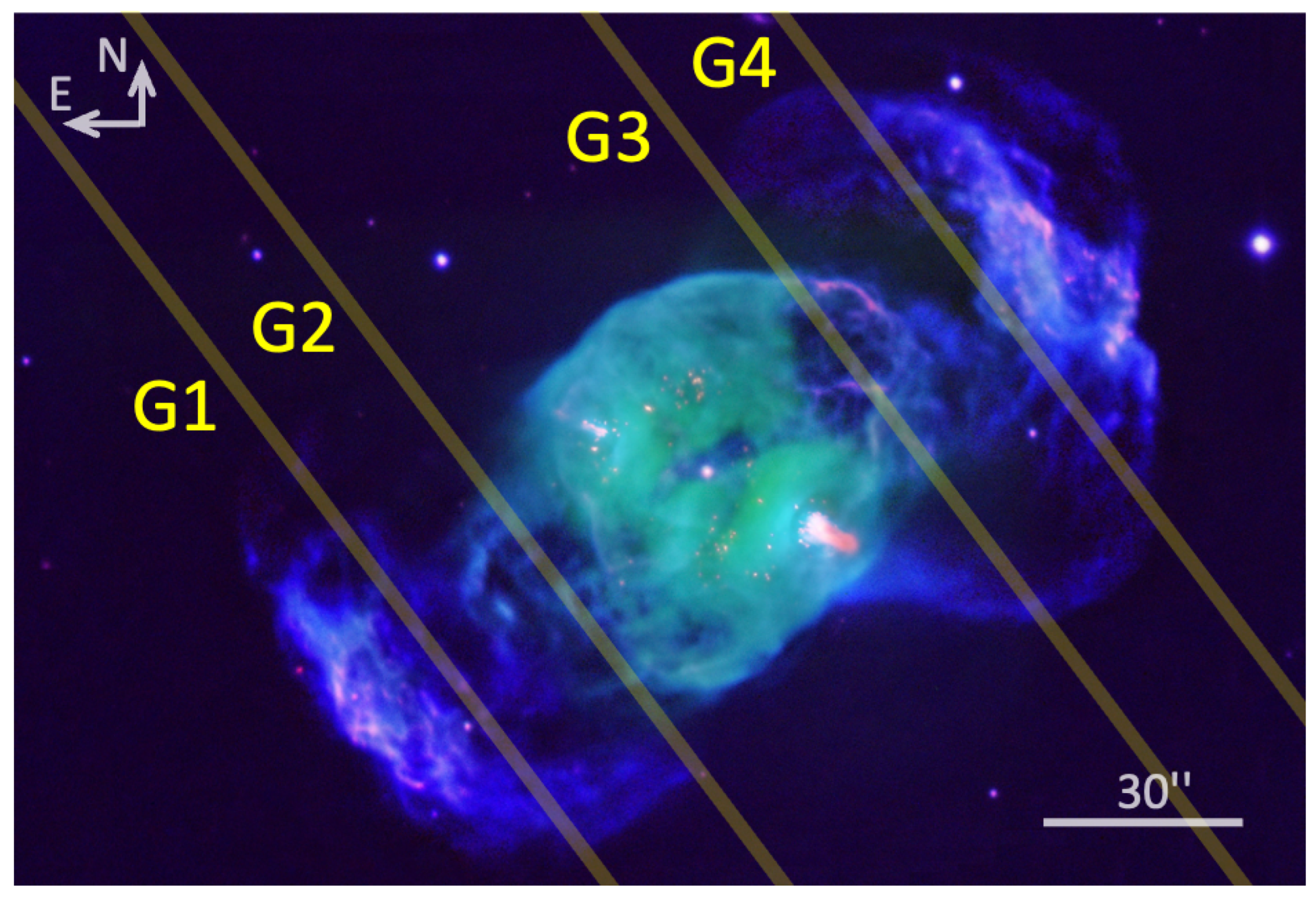
Figure 5 presents the PV maps corresponding to slits G1, G2, G3, and G4. These slits were observed at a °, crossing regions outside the main shell, which manifest as distinct lobes or large bubbles. The PV maps for G1 and G2 exhibit a predominance of the blue component, whereas for G3 and G4, the red component is more pronounced. Specifically, for G1, the emission spans approximately 66 arcsec, with expansion velocities ranging from 35 km s−1 (NE) to 63 km s−1 (SW), with the red velocity component being notably marginal.
The counterpart of G1 on the NW lobe is slit G4. A comparable structure is discerned, with a slight expansion in the SW region, manifesting a velocity of km s−1, which escalates towards the NE to approximately 58 km s−1. It is imperative to interpret this latter value with caution, as the blue component tends to attenuate, eventually vanishing in this direction. This PV map also reveals a faint, stationary emission at +18 km s−1in the NE extremity, extending over 10 arcsec. The total emission of this slit spans 82 arcsec.
As illustrated in Figure 4, slits G2 and G3 intersect the complex transition region between the barrel-like structure and the outer “lobes”. Both PV diagrams display a pronounced expansion pattern that subsequently decreases in amplitude. In the case of G2, the strongest expansion is directed toward the southwest (SW) along the slit and reaches km s−1. The blue component decreases to 22 km s−1 before appearing to increase once again. The red component vanishes when the expansion reaches its minimum. Additionally, there is a stationary emission centred at km s−1. The total emission spans 42 arcsec. The PV map for G3 reveals the largest expansion of 69 km s−1, with another of 27 km s−1 towards the SW along the slit. This slit also intersects a portion of the SW lobe, displaying a faint emission at the systemic velocity. Marginal emission is slightly observed towards the northeast (NE), but it is not possible to ascertain its expansion.
4. Discussion
4.1. The Morpho-Kinematic Model of NGC 2371
In order to further investigate the morphogenesis of NGC 2371, we produced a model using the 3D modelling tool for astrophysics, ShapeX Ver. 3.5.1 [27]. This software allows the user to define different structures with velocity patterns to produce synthetic images and PV diagrams that are then compared with those obtained from observations. A good model is evaluated by its ability to simultaneously reproduce both the observed PV diagrams and the nebular image. Our proposal is to obtain the fundamental structures, not in detail, given that in some cases there are insufficient elements to reach the microstructures. Guided by the velocity structure suggested by Gómez-González et al. [20] (see Figure 11 in that paper), we started by adopting axisymmetrical structures for NGC 2371.
To model the nebula, we use the ShapeX software in an interactive and iterative manner. Our procedure is described in detail in Appendix B. When applied to our data, we model the [O iii] Å emission in both the direct image and the PV maps, adopting an elliptical shell oriented SE–NW in the plane of the sky. Its major axis is inclined, with the NW side redshifted and the SE side blueshifted. We will refer to this ellipsoidal shell as the “barrel”, and we treat its polar regions as separate structures, hereafter referred to as the “NW cap” and the “SE cap”. In addition to these structures, we propose a system of bipolar lobes with its major axis slightly misaligned with the corresponding major axis of the barrel. Unlike most PNe with bipolar morphology, the ends of the lobes need to be spatially extended to match what we observe in the direct image, resulting in a wide waist. After the completion of the [O iii] emission model, we proceed to propose a structure for the internal knots emitting in [N ii] Å.
These low-excitation [N ii]-emitting knots were modelled as small, nearly aligned cylinders, corresponding to collimated ejections with slightly different distances with respect to the geometrical centre. The eastern knot was placed at °, with an inclination of °, and a deprojected velocity of km s−1. In contrast, the brightest knot, located to the west, was modelled with °, an inclination of °, and a deprojected velocity of km s−1. The nature of these structures will be discussed in the following section.
Table 2 summarises the morpho-kinematic characteristics of all the proposed structures, including their spatial and kinematic variables after derojection. For a detailed explanation of how these parameters were derived, we refer the reader to Appendix B. In this table, the lobes correspond to the full bipolar structure. and denote the semi-major and semi-minor axes, respectively, while and are the polar and equatorial expansion velocities, relative to the systemic velocity. For the “barrel”, is not applicable due to its truncated major axis, whereas does not apply to the caps and knots. represents the proportionality constant of the homologous velocity law adopted for each structure, while corresponds to the kinematical age taken from variables measured on the model, using the formalism from [28] as well as the value of distance obtained from the Gaia data mentioned before [18].
4.2. The Brilliant Knots in [N ii]
The most brilliant knots in [N ii] are not fully aligned themselves. One possible interpretation of this configuration is that the two knots are uncorrelated, as they are not fully aligned and exhibit different velocities. Gómez-Gonález et al. [20] argue that the shape of the [N ii]-emitting clumps is more consistent with that of photo-evaporative flows instead of jet-like features. However, the high velocity of (at least) the Easter clump challenges this idea.
An alternative interpretation could be that these knots represent a pair of bipolar, high-velocity jets that were originally aligned (their misalignment on the sky is around 10°). As a hypothesis, we propose that this emission corresponds to a pair of jets, originally ejected in opposite directions at the same velocity. Given the intense emission in [N ii] from these knots, we assume that they result from shocks caused by the bipolar jet interacting with the inner shell. Consequently, their apparent distance from the central star to their current position corresponds to the projected distance between the star and the inner shell, which is determined from the images. We can then deproject this element to obtain the inclination angle of each knot with respect to the line of sight, allowing us to deproject each velocity vector. With this information, we estimated a 3D angular misalignment of both vectors of °. The results of using this hypothesis are presented in Table 2.
The East jet has a deprojected velocity of 75 km s−1, while the West jet, which is the brightest, is also much slower ( km s−1). These features may result from the interaction of a high-velocity jet with circumstellar matter. Given the electron densities of the West jet ( cm−3) and its surroundings ( cm−3), obtained by Gómez-González et al. [20], we can reasonably estimate, using basic momentum conservation equations (see Appendix C), that a mass element could decelerate from 75 km s−1 to 20 km s−1. Thus, the slower velocity of 20 km s−1 can be explained by a deviation from the original direction, which is consistent with the observed loss of alignment. We recognise that this is a rather simple explanation. However, the small angular separation of °, its strong intensity in [N ii], and the consistency of the density estimates justify a more detailed modelling of this feature, which lies beyond the scope of the present work. Our working hypothesis is that the jets were originally ejected along a symmetry axis passing through the central star, with an initial velocity of at least 75 km s−1. For this reason, we do not regard the kinematical age of 7900 yr for the W jet as a robust value
The resulting ShapeX model, incorporating all proposed structures, is presented in Figure 6. It provides a satisfactory reproduction of the PV diagrams. In Figure 7, the synthetic spectra derived from the model are displayed superimposed on observed PV diagrams selected from Figure 3 and Figure 5, illustrating the consistency between the observations and the model.
4.3. The Origin of NGC 2371
The morpho-kinematic analysis presented in this work provides important clues to the origin and evolutionary history of NGC 2371. The different structural components show a wide range of kinematical ages: the inner barrel ( yr), the caps (–2600 yr), and the bipolar lobes ( yr). This spread suggests that the nebula did not form in a single, instantaneous ejection but rather through multiple episodes of mass loss and shaping.
The bipolar lobes are very likely the oldest structure in NGC 2371, which might have formed as a result of the main ejection during the transition of the progenitor star from the AGB to the post-AGB phase. Interestingly, the morphology of the lobes suggests that this structure was decelerated during the outflow, possibly through interaction with the surrounding medium.
Within the estimated uncertainties, the inner barrel and its associated caps seem to have formed as a result of another mass-ejection event; notably, such a secondary ejection might be linked to the same process that produced the current H-deficient [WR] characteristics of the CS of NGC 2371. It is currently accepted that [WR] stars originate from the born-again scenario [29,30], in which the CS of a PN undergoes a late thermal pulse after leaving the thermally-pulsating AGB phase; during this episode, the surface H is converted into He and C and violently expelled into the old PN, naturally giving rise to a double-shell PN morphology [31]. Finally, the star evolves into a second post-AGB phase, developing once again a fast stellar wind and a high-ionising photon flux.
The caps projected on the tips of the barrel may trace subsequent, somewhat more collimated outflows that have influenced the outermost regions of the nebula. For the SE cap, no clear morphological or kinematical differences are found with respect to the barrel. The only obvious distinction is the lower surface brightness of both caps relative to the barrel. In contrast, the NW cap not only expands more rapidly but also appears slightly detached from the barrel. This asymmetry is consistent with episodic and not strictly symmetric bipolar ejections; however, local conditions in the circumstellar environment, such as density gradients or anisotropies in the surrounding medium, could likewise have affected the NW cap differently. These properties seem to be consistent with what is observed in other born-again PNe, where the inner shell is not completely bipolar but exhibits a collection of clumps and filaments inside the old PN [32].
Nevertheless, additional effects produced by a binary companion are also evident. The pronounced bipolar morphology of the lobes suggests that shaping by a companion played an important role prior to the formation of the barrel-like structure. Moreover, the slight misalignment between the lobes and the barrel likely reflects precession – possibly driven by binary interactions – or a change in the dominant mass-loss axis over time. For example, the bright [N ii] knots provide evidence of even later ejection events, or of jets interacting with denser circumstellar material. Their misalignment and asymmetric velocities strongly suggest episodic jet activity, possibly associated with intermittent accretion processes in a binary system. This interpretation is consistent with hydrodynamical simulations of binary-driven outflows, where collimated jets interact with pre-existing shells and produce localised distortions in morphology and kinematics e.g. [33]. An additional point to consider is that the derived kinematical ages of these knots may not directly reflect their true time of origin, but rather the significant alterations in trajectory and velocity that they have experienced. Such deviations could represent indirect evidence of their interaction with an inhomogeneous circumstellar medium or, alternatively, the imprint of variable jet-launching conditions linked to binarity.
Although there is currently no direct evidence confirming that the CS of NGC 2371 is a binary, the observational evidence presented here strongly supports this idea. Asteroseismological surveys using TESS and Kepler have demonstrated their potential to reveal pulsations and rotational modulations in PG 1159-type stars, with several objects already showing clear variability signatures e.g. [34,35]. These techniques could be applied to the nucleus of NGC 2371 to search for evidence of a companion. Moreover, binary CSs are increasingly recognised as key drivers in the formation and evolution of complex PNe e.g. [36], with confirmed examples illustrating the diverse shaping mechanisms related to binarity. Therefore, we propose that future time-domain photometry or time-resolved spectroscopy be pursued to test whether the CS of NGC 2371 shares a binary-driven evolutionary history.
Another important aspect to highlight is that the final model of NGC 2371 required the large-scale structures (the bipolar lobes and the barrel) to display surface irregularities in the form of small ridges and valleys. Interestingly, their orientations do not seem to be directly related to the flow of material expelled by the central star. This might indicate the action of additional energetic processes that locally modify both the morphology and the kinematics. Such processes could involve hydrodynamical instabilities, interaction with pre-existing circumstellar material, or even collimated outflows driven by binary interactions. The very shape of the bipolar lobes of NGC 2371 is unusual: while morphologically similar cases exist e.g. NGC 6369, [37], the differences suggest that more than one shaping mechanism may be at play. These comparisons point towards the possibility that the evolution of NGC 2371 involved additional processes beyond those accounted for in our current models, thus opening the way for future observational and theoretical studies to test these scenarios.
5. Conclusions
Our morpho-kinematic analysis of NGC 2371 shows that its present-day morphology is the outcome of multiple episodic mass-loss events rather than a single outflow. The combination of a barrel-shaped shell, extended bipolar lobes, younger polar caps, and misaligned [N ii] knots points to a complex evolutionary history. The derived kinematical ages, spanning from 1600 to 4400 years, indicate successive episodes of mass loss with different geometries and timescales.
The peculiar morphology of NGC 2371 – its nearly perpendicular bipolar lobes, bipolarity without a pronounced waist, and surface distortions that do not align with the central outflow – cannot be explained solely by standard axisymmetric wind interactions. Instead, our results indicate that a combination of factors played a decisive role in shaping this nebula: a late thermal pulse that produced the H-deficient [WR] CS, binary-driven interactions, and episodic jet activity. NGC 2371 therefore stands out as an exceptional and highly unusual PN, pointing to physical mechanisms that remain poorly understood or only marginally explored in current models of PN formation and evolution.
Author Contributions
Conceptualization, RV, JAT, LFM, GRL; methodology, RV, LFM, SA, PFG, LO, FSB; validation, GRL, LS; formal analysis, RV, SA, LFM, MAGM, LO; investigation, RV, JAT, LFM, FSB; resources, RV, LFM, SA, MAGM, PFG, LO, FSB; data curation, RV, MEC, MAGM, PFG, LO, FSB; writing—original draft preparation, RV, JAT; writing—review and editing, LFM, GRL, LS; visualization, SA, MEC, MAGM, LO, FSB; supervision, RV; project administration, RV; funding acquisition, RV, JAT, LFM, LS. All authors have read and agreed to the published version of the manuscript.
Funding
This work was supported by UNAM PAPIIT (Mexico) IN106720, IN103125, IA101622, IN102324, and IN107625 grants. LFM acknowledges support from grants PID2023-146295NB-I00 and CEX2021-001131-S funded by MCIN/AEI/10.13039/501100011033.
Data Availability Statement
The data files will be shared on request to the first author.
Acknowledgments
This study is based upon observations carried out at the Observatorio Astrónomico Nacional on the Sierra San Pedro Mártir (OAN-SPM), Baja California, Mexico. The authors thank the OAN-SPM staff, in particular the telescope operators Gastavo Melgoza (aka “Tiky”), Felipe Montalvo, and Salvador Monroy (aka “Capt. Storm”). This work has made extensive use of NASA’s Astrophysics Data System (ADS). NOIRLab iraf is distributed by the Community Science and Data Center at NSF NOIRLab, which is managed by the Association of Universities for Research in Astronomy (AURA) under a cooperative agreement with the U.S. National Science Foundation. During the preparation of this manuscript, the authors used ChatGPT 5.1 for the purposes of grammatical revision. The authors have reviewed and edited the output and take full responsibility for the content of this publication. Finally, the authors wish to dedicate this paper to the memory of Professor Roberto Machorro (UNAM), an active researcher in optics, an inspiring educator, and a tireless promoter of science outreach, who recently passed away. ¡Gracias, Profe!
Conflicts of Interest
The authors declare no conflicts of interest.
Appendix A. Additional PV Diagrams
Figure A1 shows the slit position for observational run A according to Table 1. The corresponding PV diagrams are presented in Figure A2.
Figure A1.
Same composite [O iii] image of NGC 2371 as in Figure 1, now showing the slit positions for run A. North is up and east is to the left.
Figure A1.
Same composite [O iii] image of NGC 2371 as in Figure 1, now showing the slit positions for run A. North is up and east is to the left.
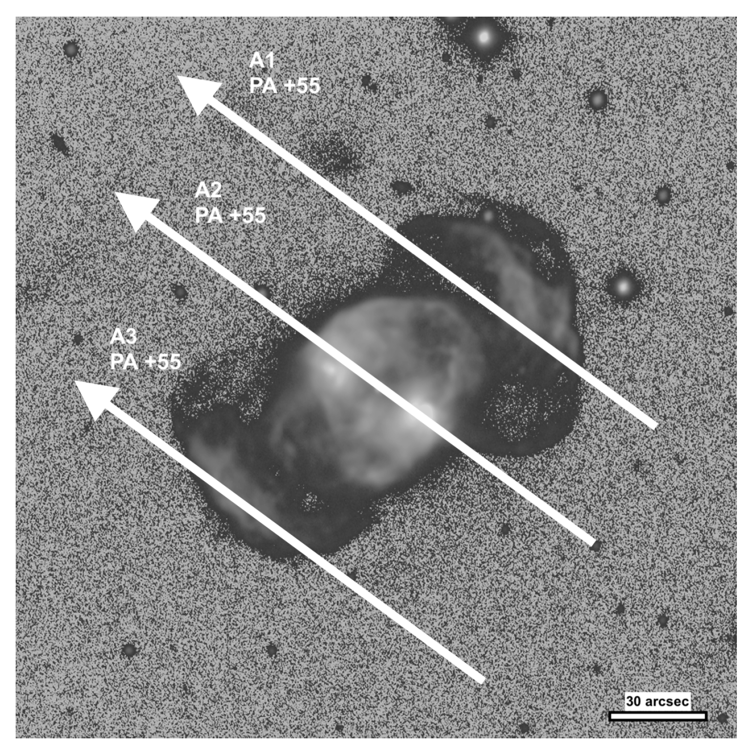
Figure A2.
The figure displays the PV diagrams from slit positions A1, A2, and A3 at PA=+55° in the [O iii] emission line. Slit A2, which crosses the central star, is presented in a logarithmic scale. The greyscale and zero position for all the spectra were chosen to improve the clarity of the image. The velocity scale is relative to the systemic velocity.

Figure A3 shows the slit position for observational run B according to Table 1. The corresponding PV diagrams are presented in Figure A4.
Figure A3.
Same as Figure A1 but for run B.
Figure A3.
Same as Figure A1 but for run B.
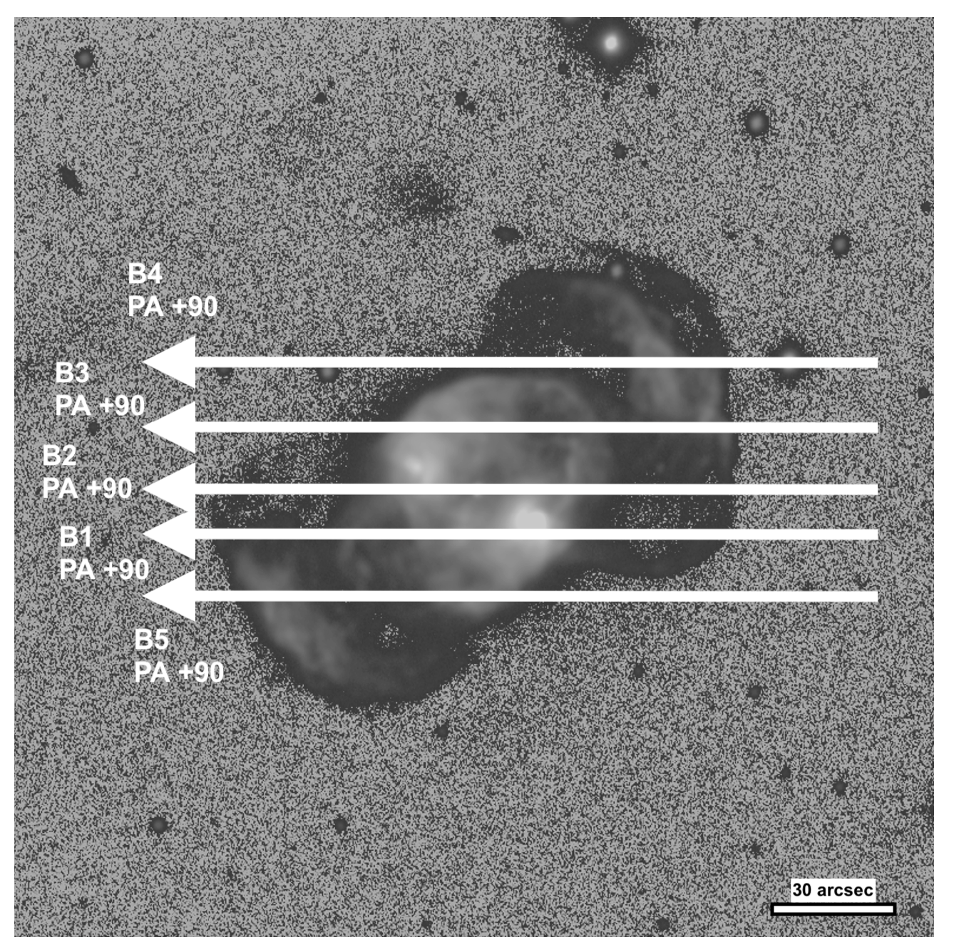
Figure A4.
This figure displays the PV diagrams from slit positions B1 to B5 at PA=+90° in the [O iii] emission line in logarithmic scale. The greyscale and zero position for all the spectra were chosen to improve the clarity of the image. The velocity scale is relative to the systemic velocity.
Figure A4.
This figure displays the PV diagrams from slit positions B1 to B5 at PA=+90° in the [O iii] emission line in logarithmic scale. The greyscale and zero position for all the spectra were chosen to improve the clarity of the image. The velocity scale is relative to the systemic velocity.
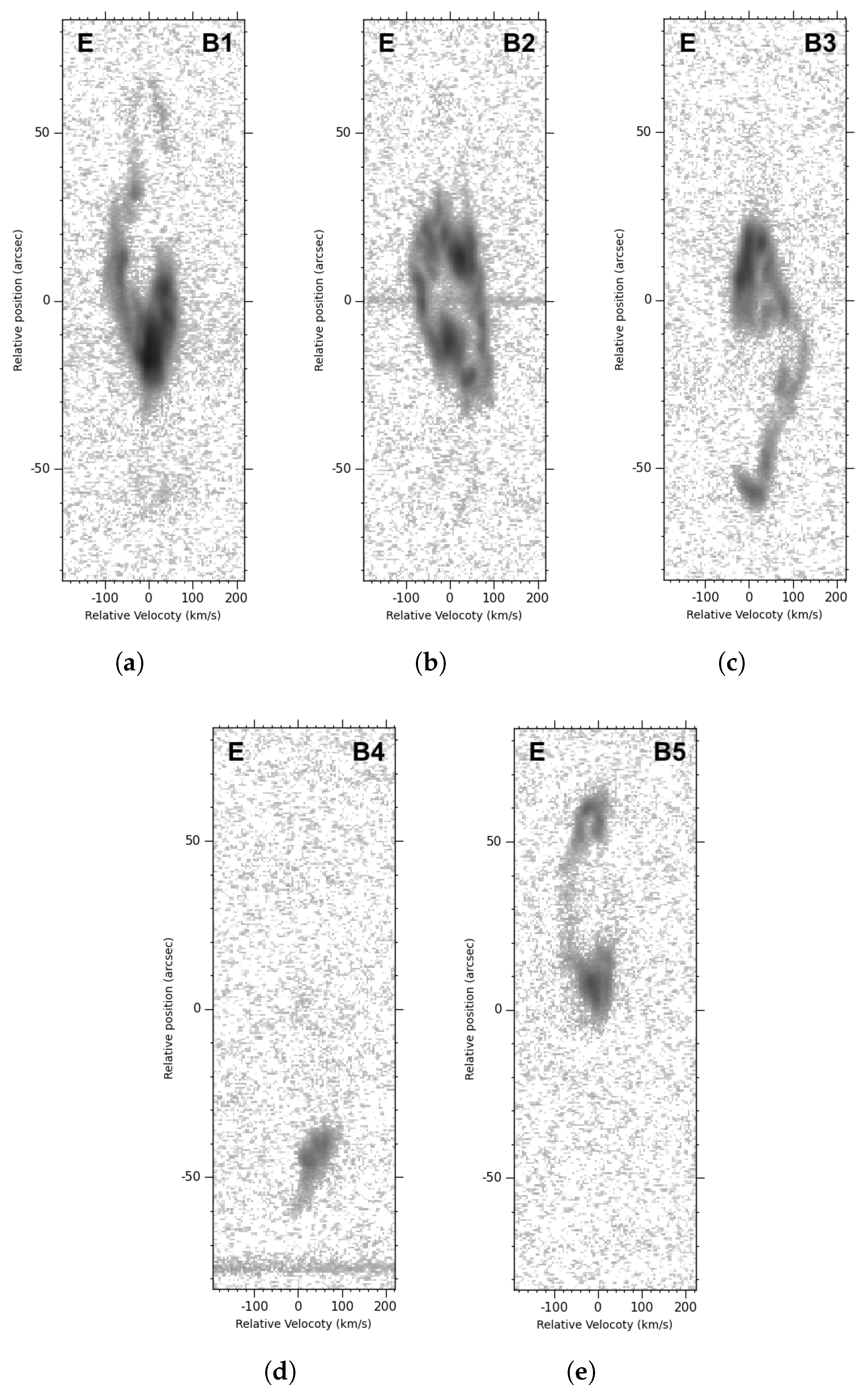
Figure A5 shows the slit position for observational run C according to Table 1. The corresponding PV diagrams are presented in Figure A6.
Figure A5.
Same as Figure A1 but for run C.
Figure A5.
Same as Figure A1 but for run C.
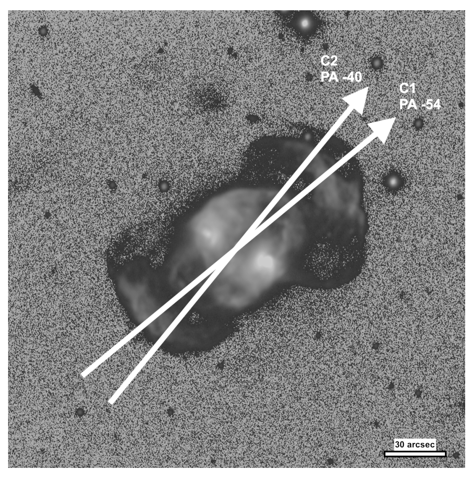
Figure A6.
PV diagrams from slit positions C1 and C2, at PA=° and PA°, respectively, in the [O iii] emission line. The greyscale was chosen to improve the clarity of both images. The velocity scale is relative to the systemic velocity, and the position is measured with respect to the central star.
Figure A6.
PV diagrams from slit positions C1 and C2, at PA=° and PA°, respectively, in the [O iii] emission line. The greyscale was chosen to improve the clarity of both images. The velocity scale is relative to the systemic velocity, and the position is measured with respect to the central star.
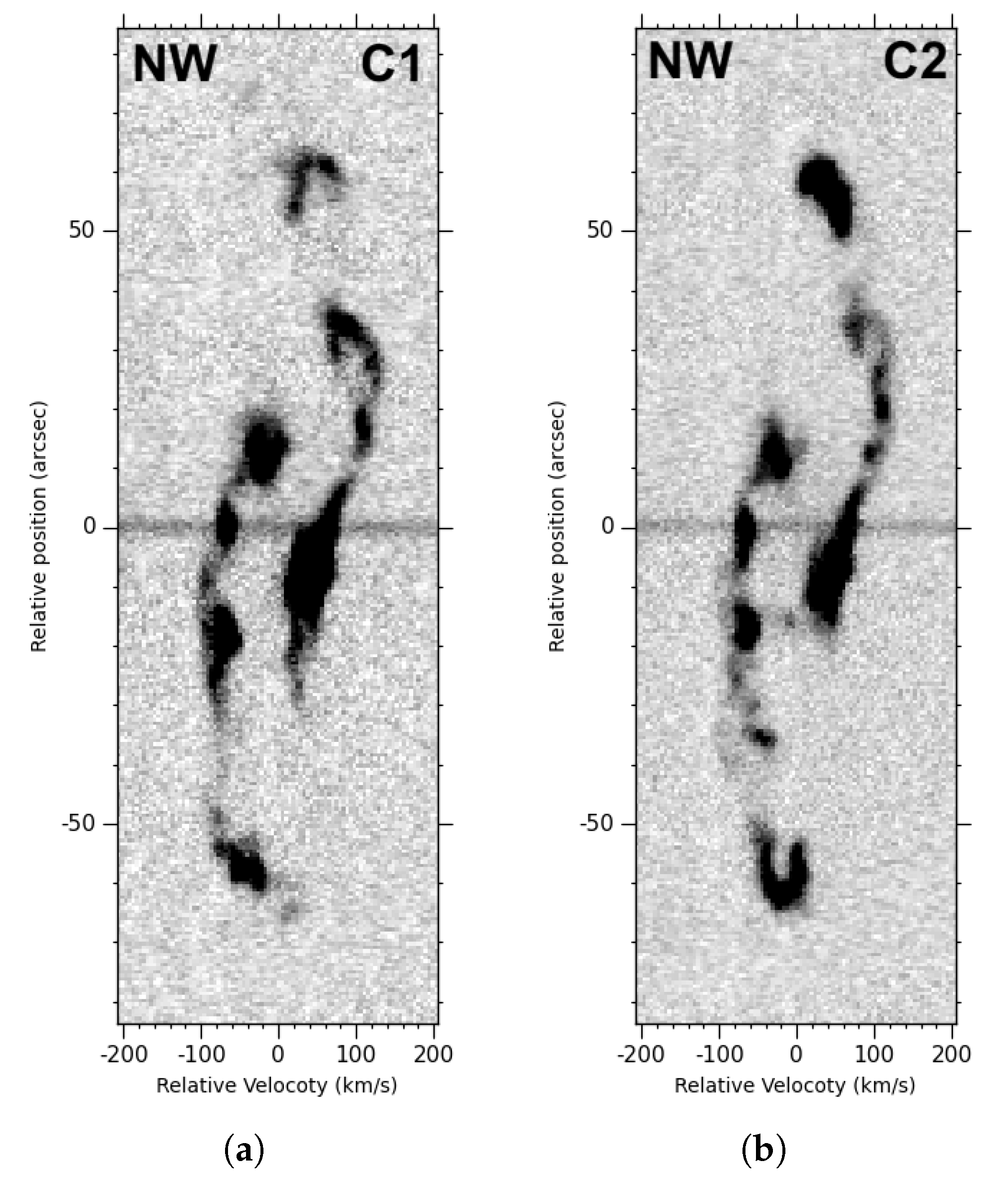
Figure A7 shows the slit position for observational run D according to Table 1. The corresponding PV diagrams are presented in Figure A8.
Figure A7.
Same as Figure A1 but for run D.
Figure A7.
Same as Figure A1 but for run D.
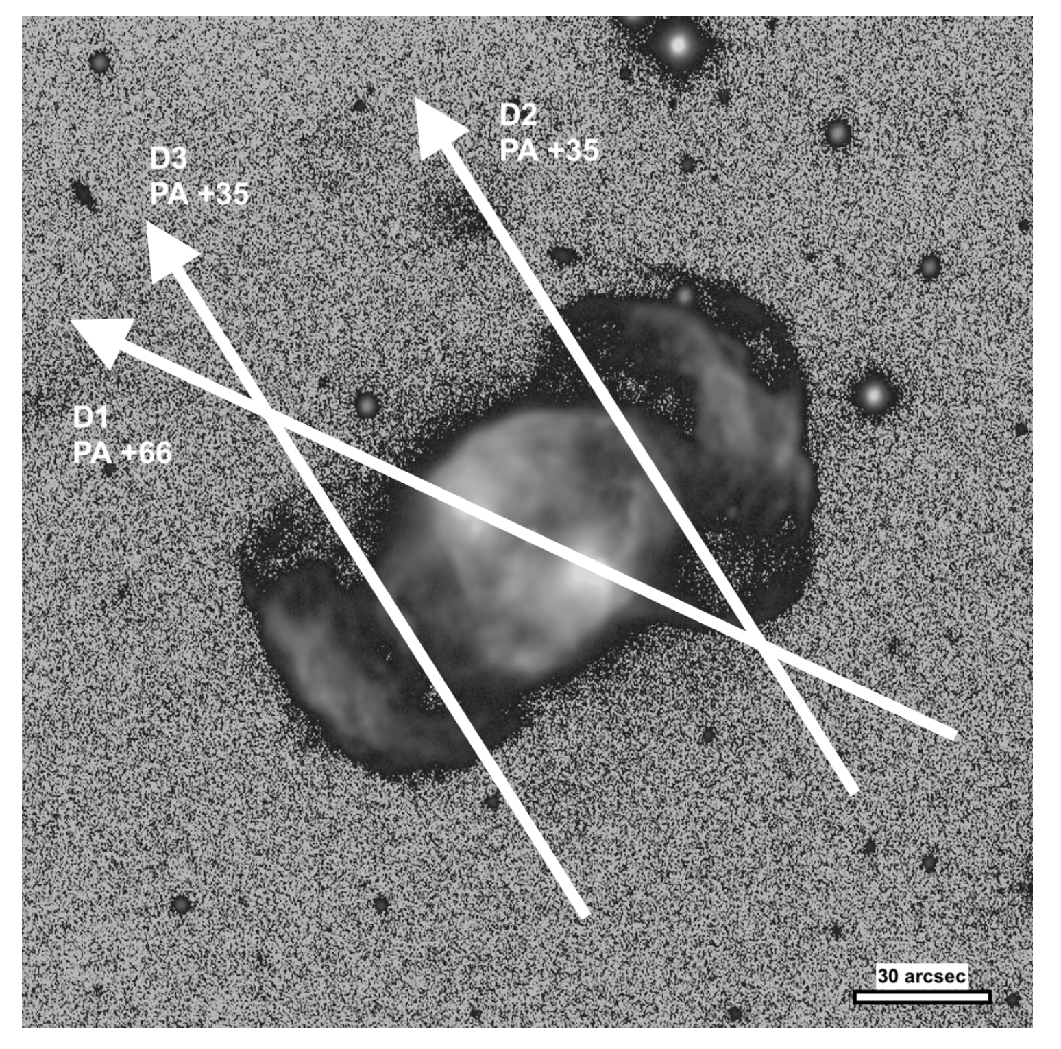
Figure A8.
The figure displays the PV diagrams from slit positions at PA=+66° (D1, crossing the central star) and PA=+35° (D2 and D3, crossing the upper and lower regions, respectively) in the [O iii] emission line. A logarithmic scale for intensity was used for the three spectra. The greyscale and zero position were chosen to improve the clarity of each image. The velocity scale is relative to the systemic velocity.
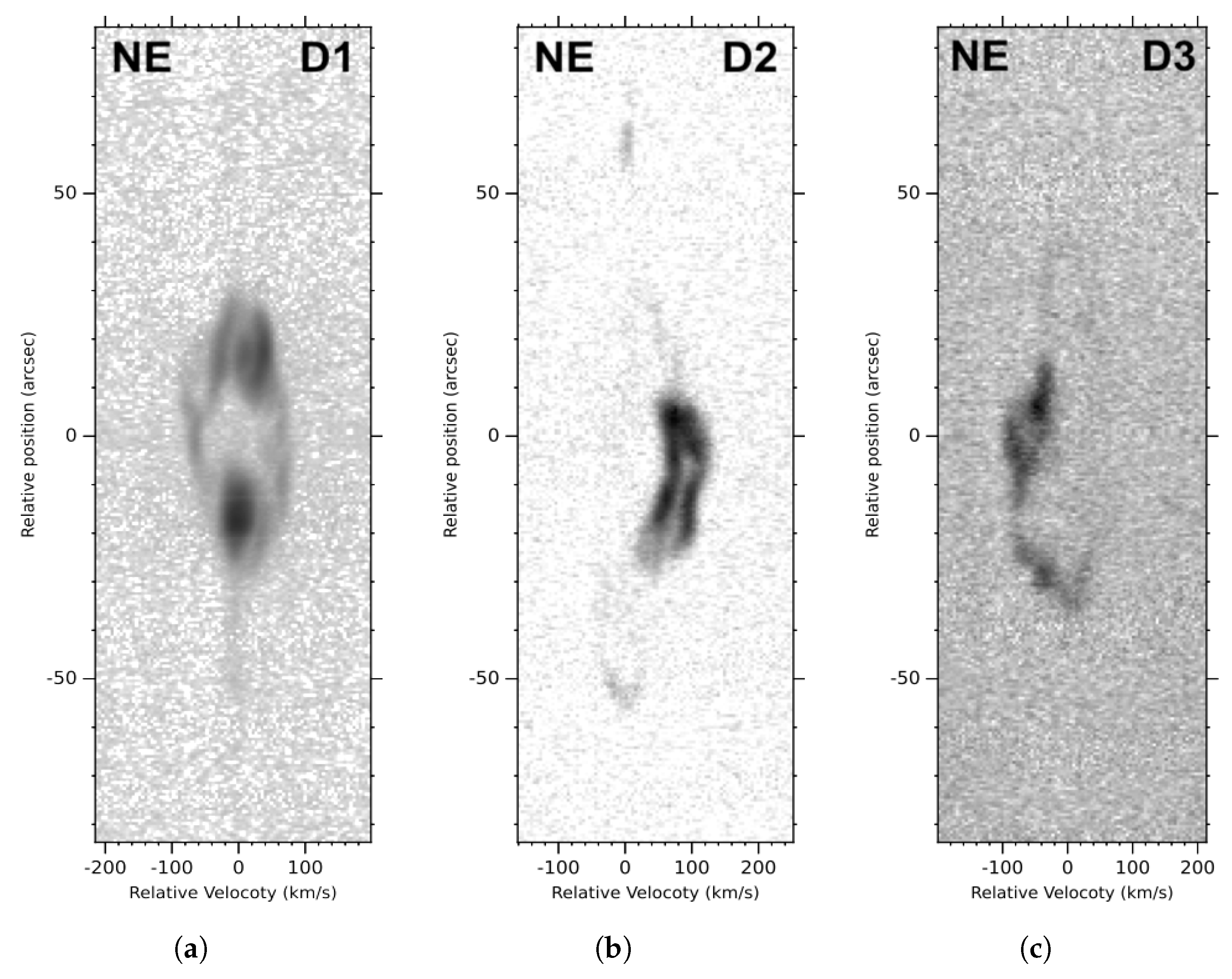
Figure A9 shows the slit position for observational run E according to Table 1. The corresponding PV diagrams are presented in Figure A10 and Figure A11.
Figure A9.
Same as Figure A1 but for run E.
Figure A9.
Same as Figure A1 but for run E.
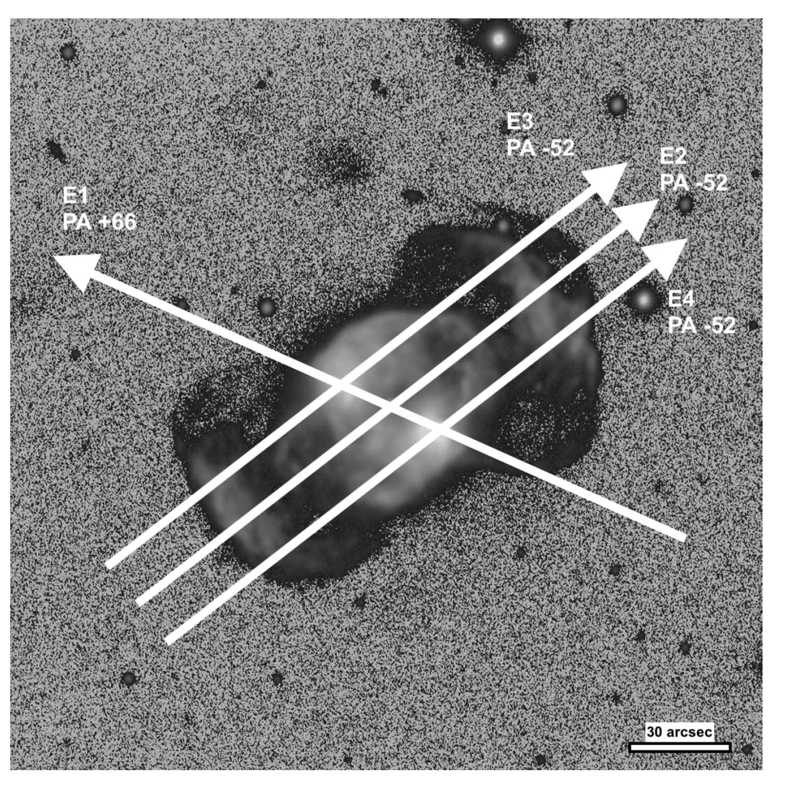
Figure A10.
PV diagrams from slit positions E1 at PA=+66° in the H+He iiÅ and [N ii]Å emission lines. The greyscale has been chosen to improve the clarity of each spectrum. The velocity scale is referenced to the systemic velocity, and positions are relative to the central star.
Figure A10.
PV diagrams from slit positions E1 at PA=+66° in the H+He iiÅ and [N ii]Å emission lines. The greyscale has been chosen to improve the clarity of each spectrum. The velocity scale is referenced to the systemic velocity, and positions are relative to the central star.
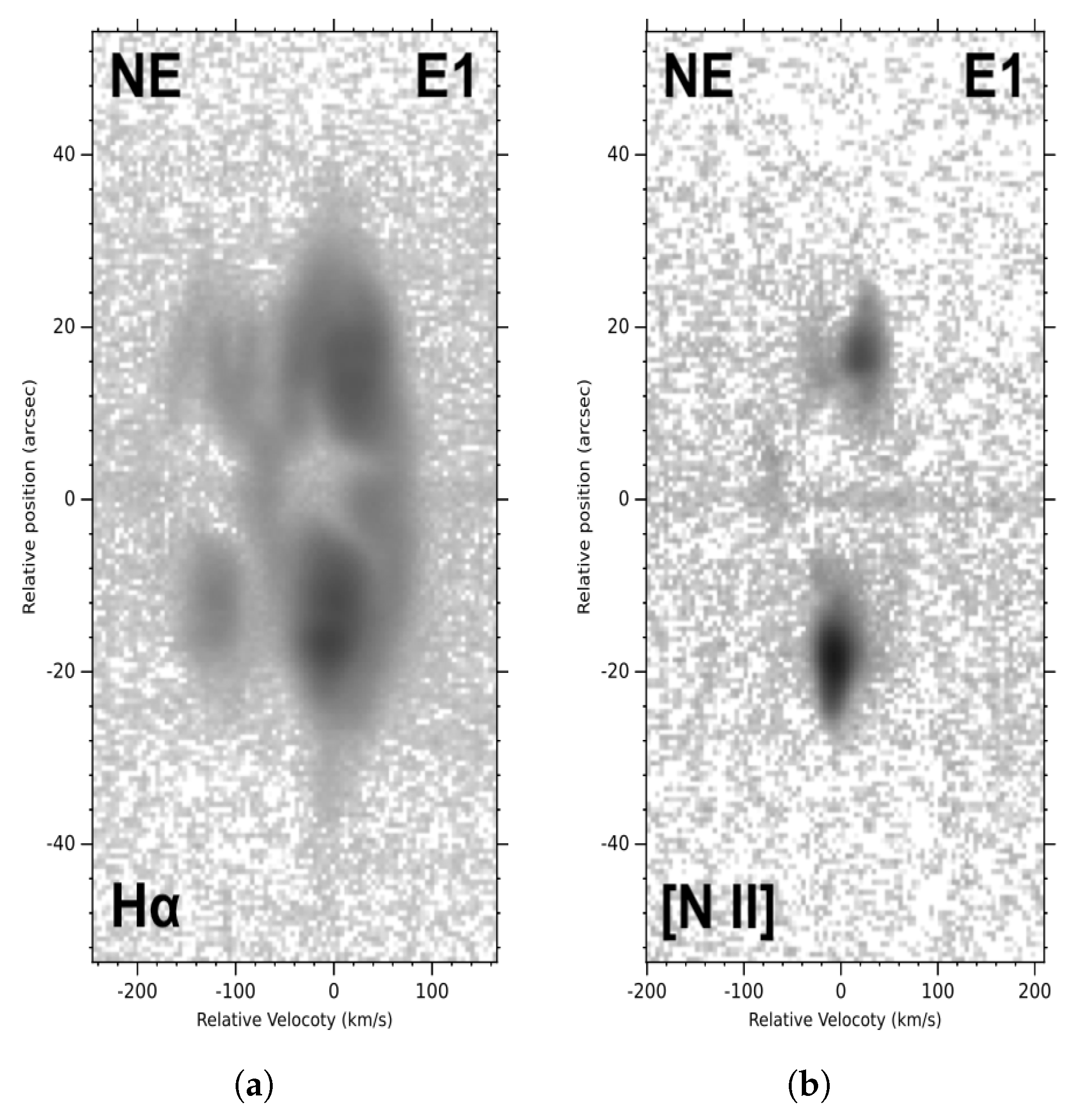
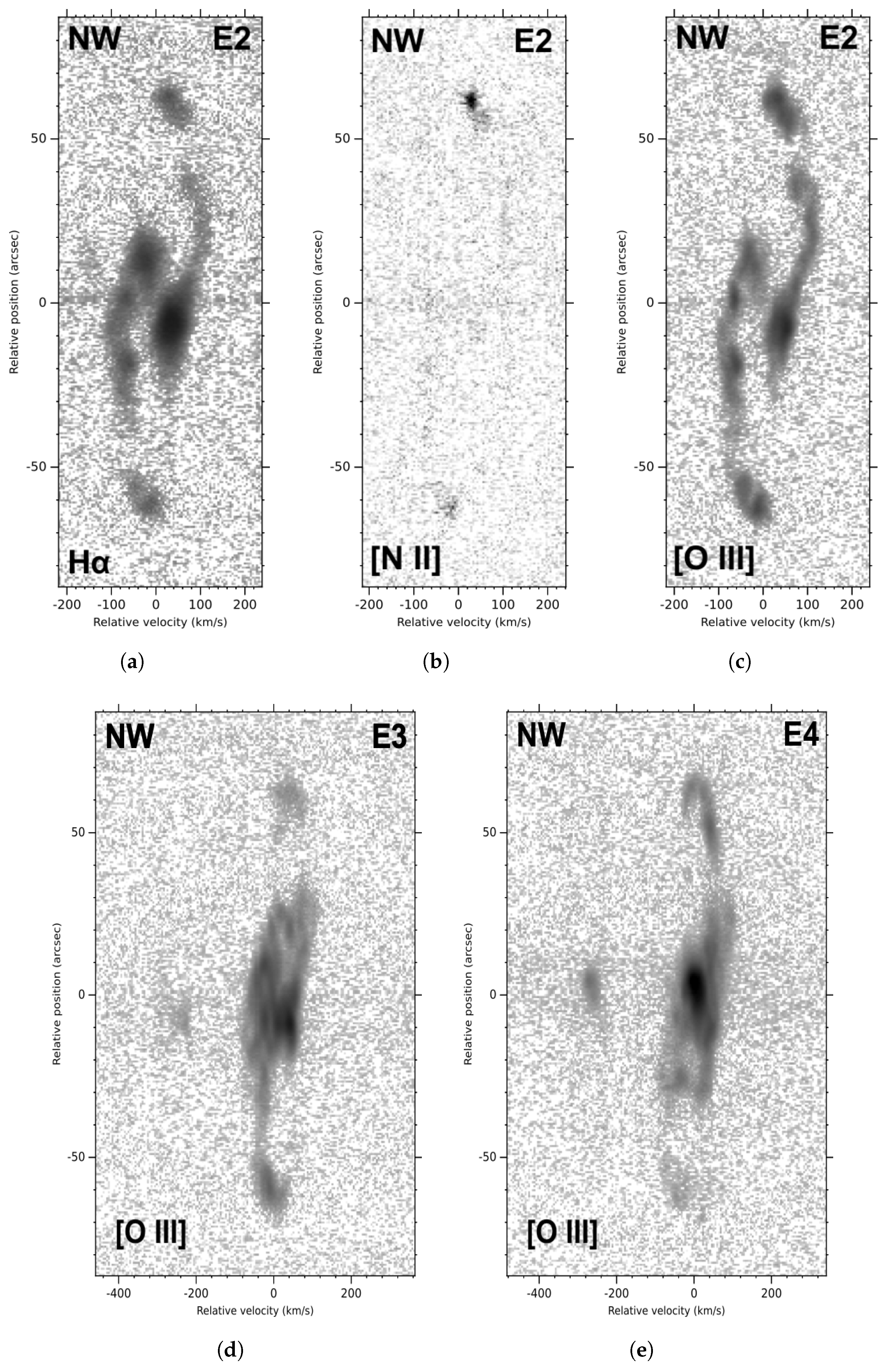
Figure A11.
Up: PV diagrams derived from slit position E2 at °, intersecting the central star, in the H, [N ii]Å, and [O iii]Å emission lines. Bottom: PV diagrams derived from slit positions E3 and E4 at °, crossing the [O iii] maxima (E and W, respectively). In all the PV maps, the greyscale was chosen to improve the clarity of each image. The velocity scale is relative to the systemic velocity and the position is measured with respect to the central star.
Appendix B. Modelling Structures in ShapeX
To avoid confusion, we find it important to outline the methodology used in ShapeX, which we have refined through our previous works e.g. [28,38,39,40]. In these studies, we adopted an interactive and iterative approach to construct models of nebular structures. The procedure can be summarised as follows:
- In most cases, the process begins by defining a sphere whose polar axis is initially oriented along the N–S direction.
- The sphere is then rotated so that its polar axis attains a position angle (PA) consistent with the orientation of the main axis of the structure to be modelled.
- At this stage, the modifiers SIZE or SQUEEZE are applied to transform the sphere into an ellipsoid or even into a bipolar structure. In some cases, only a section of these surfaces is employed to reproduce the observed morphology. For example, an ellipsoid may be used to represent a cap, but this does not imply the existence of the entire ellipsoid, only the region that matches the observed feature. This approach allows us to estimate both the distance from the geometric centre to the cap and to assign a velocity law consistent with its expansion.
- Once the synthetic structure resembles the morphology seen in direct imaging, a velocity law and an inclination angle with respect to the line of sight are introduced. These parameters are adjusted iteratively, along with the size and orientation, until the model reproduces the relevant portion of the PV diagram while maintaining consistency with the direct image.
- The same procedure is then repeated for each additional structure. In practice, it is often more effective to begin with a single PV diagram and, once a convincing fit is obtained, to test whether it also reproduces other PV diagrams. This process is continued until a robust final model is reached, in which all structures reproduce satisfactorily both the morphological and kinematic characteristics observed in the images and spectra.
- Using ShapeX as an analysis tool is also very powerful. For example, once an elliptical or bipolar structure has been defined and an inclination angle and velocity law have been assigned, the model can be rotated to view the nebula pole-on, and synthetic spectra can be extracted to directly measure the deprojected polar velocity. Likewise, by rotating the model so that the main axis is perpendicular to the line of sight, the deprojected equatorial expansion velocity can also be measured.
Appendix C. Calculations
First-order approximation of a fully inelastic collision: Consider the collision between the West Jet (J) and a dense gas region (R) as fully inelastic. By applying the conservation of momentum, the equation can be expressed as:
where and are the masses of the jet and the dense region, respectively; is the initial velocity of the jet, and is its final velocity post-collision. Assuming that the dense region is initially at rest (), and using the definition of density (mass/volume), we derive:
Following Gómez-González et al. [20], we adopt densities of cm−3 and cm−3. For the velocities, we use the values derived in this work, assuming that the deflected jet initially had a velocity of km s−1 and was slowed down to km s−1. Therefore, the volume ratio of the interacting regions can be approximated as:
Assuming forms a cylinder with the same radius as the ballistic knot that constitutes the jet (r), and the length of the cylinder corresponds to the thickness of the shell , we obtain the ratio:
Given that the shell thickness was modelled at 15 arcsec and the original radius of the jet at approximately 2 arcsec, the actual ratio is:
corresponding to an error of approximately 17 to 20%. We consider that this result implies that this interpretation is feasible given our data and our final model.
References
- Ramstedt, S.; Vlemmings, W. H. T.; Doan, L.; et al. 2020, DEATHSTAR: Nearby AGB stars with the Atacama Compact Array I. CO envelope sizes and asymmetries: A new hope for accurate mass-loss-rate estimates, A&A, 640, A133. [CrossRef]
- Scicluna, P.; Kemper, F.; McDonald, I.; et al. 2022, The Nearby Evolved Stars Survey II: Constructing a volume-limited sample and first results from the JCMT, MNRAS, 512, 1091. [CrossRef]
- Kwok, S. 2000, The Origin and Evolution of Planetary Nebulae, Cambridge Astrophysics Series, Vol. 33, Cambridge University Press, Cambridge.
- De Marco, O. 2009, The Origin and Shaping of Planetary Nebulae: Putting the Binary Hypothesis to the Test, PASP, 121, 316. [CrossRef]
- Sahai, R.; Morris, M. R.; Villar, G. G. 2011, Young Planetary Nebulae: Hubble Space Telescope Imaging and a New Morphological Classification System, AJ, 141, 134. [CrossRef]
- Ivanova, N.; Justham, S.; Chen, X.; et al. 2013, Common envelope evolution: where we stand and how we can move forward, A&AR, 21, 59. [CrossRef]
- Chamandy, L.; Blackman, E. G.; Frank, A.; et al. 2020, Common envelope evolution on the asymptotic giant branch: unbinding within a decade, MNRAS, 495, 4028. [CrossRef]
- García-Segura, G.; Taam, R. E.; Ricker, P. M. 2022, Common-envelope shaping of planetary nebulae IV: From protoplanetary to planetary nebula, MNRAS, 517, 3822. [CrossRef]
- López-Cámara, D.; De Colle, F.; Moreno Méndez, E.; et al. 2022, Jets in common envelopes: a low-mass main-sequence star in a red giant, MNRAS, 513, 3634. [CrossRef]
- Ondratschek, P. A.; Röpke, F. K.; Schneider, F. R. N.; et al. 2022, Single-degenerate Type Ia supernovae from common envelope evolution, A&A, 660, L8. [CrossRef]
- Rechy-García, J. S.; Toalá, J. A.; Guerrero, M. A.; et al. 2022, The common envelope origins of the fast jet in the planetary nebula M 3–38, ApJL, 933, L24. [CrossRef]
- Henney, W. J.; López, J. A.; García-Díaz, M. T.; et al. 2021, Five axes of the Turtle: symmetry and asymmetry in NGC 6210, MNRAS, 502, 1070. [CrossRef]
- Rodríguez-González, J. B.; Toalá, J. A.; Sabin, L.; et al. 2022, Adjusting the bow-tie: a morpho-kinematic study of NGC 40, MNRAS, 515, 1557. [CrossRef]
- Pottasch, S. R.; Gathier, R.; Gilra, D. P.; et al. 1981, The ultraviolet spectrum of the planetary nebula NGC 2371 and its exciting star, A&A, 102, 237.
- Kaler, J. B.; Stanghellini, L.; Shaw, R. A. 1993, NGC 2371: a high-excitation planetary nebula with an O VI nucleus, A&A, 279, 529.
- Ramos-Larios, G.; Phillips, J. P. 2012, The structure of the planetary nebula NGC 2371 in the visible and mid-infrared, MNRAS, 425, 1091. [CrossRef]
- Hajduk, M.; Haverkorn, M.; Shimwell, T.; et al. 2021, Evidence for cold plasma in planetary nebulae from LOFAR observations, ApJ, 919, 121. [CrossRef]
- Bailer-Jones, C. A. L., Rybizki, J., Fouesneau, M., et al. 2021, Estimating Distances from Parallaxes. V. Geometric and Photogeometric Distances to 1.47 Billion Stars in Gaia Early Data Release 3, AJ, 161, 3, 147. [CrossRef]
- Sabbadin, F.; Bianchini, A.; Hamzaoglu, E. 1982, Spatial–kinematical models for planetary nebulae: NGC 2371–2, A&AS, 50, 523.
- Gómez-González, V. M. A.; Toalá, J. A.; Guerrero, M. A.; et al. 2020, Planetary nebulae with Wolf–Rayet-type central stars I: The case of the high-excitation NGC 2371, MNRAS, 496, 959. [CrossRef]
- Olguín, L.; Vázquez, R.; Cook, R.; et al. 2002, Physical Conditions and Chemical Structure of the PNe NGC 2440 and NGC 2371-72, Revista Mexicana de Astronomía y Astrofísica Conference Series, 12, 172.
- Ayala, S.; Vázquez, R.; Miranda, L. F.; et al. 2005, NGC 2371: Mapping its physical and kinematic structure, in Planetary Nebulae as Astronomical Tools, AIP Conf. Proc., 804, 95. [CrossRef]
- Meaburn, J.; López, J. A.; Gutiérrez, L.; et al. 2003, The Manchester Echelle Spectrometer at the San Pedro Mártir Observatory (MES–SPM), RevMexA&A, 39, 185.
- Tody, D. 1986, The IRAF Data Reduction and Analysis System, Proc. SPIE, 627, 733. [CrossRef]
- Tody, D. 1993, IRAF in the Nineties, in Astronomical Data Analysis Software and Systems II, ASP Conf. Ser., 52, 173.
- Fitzpatrick, M.; Placco, V.; Bolton, A.; et al. 2025, Modernizing IRAF to Support Gemini Data Reduction, ASPCS, 541, 461. [CrossRef]
- Steffen, W.; Koning, N.; Wenger, S.; Morisset, C.; Magnor, M. 2011, Shape: A 3D modeling tool for astrophysics, IEEE Trans. Vis. Comput. Graphics, 17, 454. [CrossRef]
- Guillén, P. F.; Vázquez, R.; Miranda, L. F.; Zavala, S.; Contreras, M. E.; Ayala, S.; Ortiz-Ambriz, A. 2013, Multiple outflows in the planetary nebula NGC 6058, MNRAS, 432, 2676. [CrossRef]
- Schoenberner, D. 1979, Asymptotic giant branch evolution with steady mass loss, A&A, 79, 108.
- Iben, I., Kaler, J. B., Truran, J. W., et al. 1983, On the evolution of those nuclei of planetary nebulae that experiencea final helium shell flash, ApJ, 264, 605. [CrossRef]
- Toalá, J. A., Lora, V., Montoro-Molina, B., et al. 2021, Formation and fate of the born-again planetary nebula HuBi 1, MNRAS, 505, 3, 3883. [CrossRef]
- Fang, X., Guerrero, M. A., Marquez-Lugo, R. A., et al. 2014, Expansion of Hydrogen-poor Knots in the Born-again Planetary Nebulae A30 and A78, ApJ, 797, 2, 100. [CrossRef]
- Zou, Y.; Frank, A.; Chen, Z.; Reichardt, T.; De Marco, O.; Blackman, E. G.; Nordhaus, J.; et al. 2020, Bipolar planetary nebulae from outflow collimation by common envelope evolution, MNRAS, 497, 2855. [CrossRef]
- Córsico, A. H.; Althaus, L. G.; Miller Bertolami, M. M.; et al. 2021, White-Dwarf Asteroseismology with the Kepler Space Telescope, Frontiers in Astronomy and Space Sciences, 8, 631132. [CrossRef]
- Oliveira da Rosa, G.; et al. 2022, Kepler and TESS Observations of PG 1159-035, ApJ, 936(2), 187. [CrossRef]
- Jones, D. 2020, Binary Central Stars of Planetary Nebulae, Galaxies, 8, 33. [CrossRef]
- Ramos-Larios, G.; Guerrero, M. A.; Vázquez, R.; Phillips, J. P. 2012, Optical and infrared imaging and spectroscopy of the multiple-shell planetary nebula NGC 6369, MNRAS, 420, 1977. [CrossRef]
- Vázquez, R. 2012, Bubbles and Knots in the Kinematical Structure of the Bipolar Planetary Nebula NGC 2818, ApJ, 751, 116. [CrossRef]
- Gómez-Muñoz, M. A.; Vázquez, R.; Sabin, L.; Olguín, L.; Guillén, P. F.; Zavala, S.; Michel, R. 2023, The origin of the planetary nebula M 1–16: a morpho-kinematic and chemical analysis, A&A, 676, A101. [CrossRef]
- Friederich-Hidalgo, A.; Torres, R. M.; Soto-Badilla, F.; Medina-Leal, C. A.; Gil-Gallegos, S. S.; Íñiguez-Garín, E.; Vázquez, R. 2025, Tracing the ISM–PN interaction: a morphokinematic study of Abell 71, MNRAS, 541, 3932. [CrossRef]
Figure 1.
Composite [O iii] image of NGC 2371. A reverse greyscale image is saturated to enhance the faint outer structures of the nebula, while a standard greyscale image is superposed to highlight the inner regions. The main apparent structures are labelled; this nomenclature is used in the following sections.
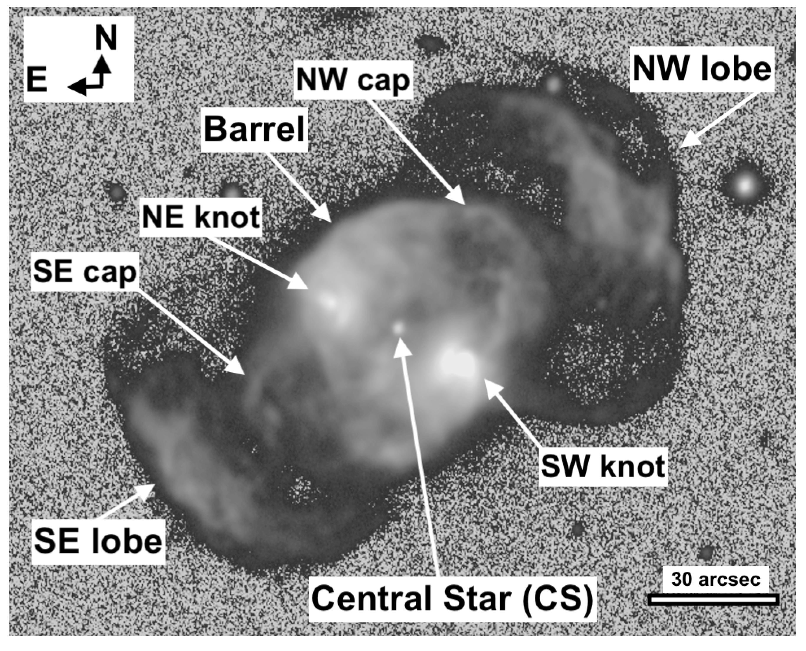
Figure 2.
Colour-composite image of NGC 2371. The red, green, and blue channels correspond to the [N ii], H, and [O iii] optical images presented in Gómez-González et al. [20] (Figure 1). Slit positions are overlaid on the image for the run F (left). Refer to Table 1 for details.
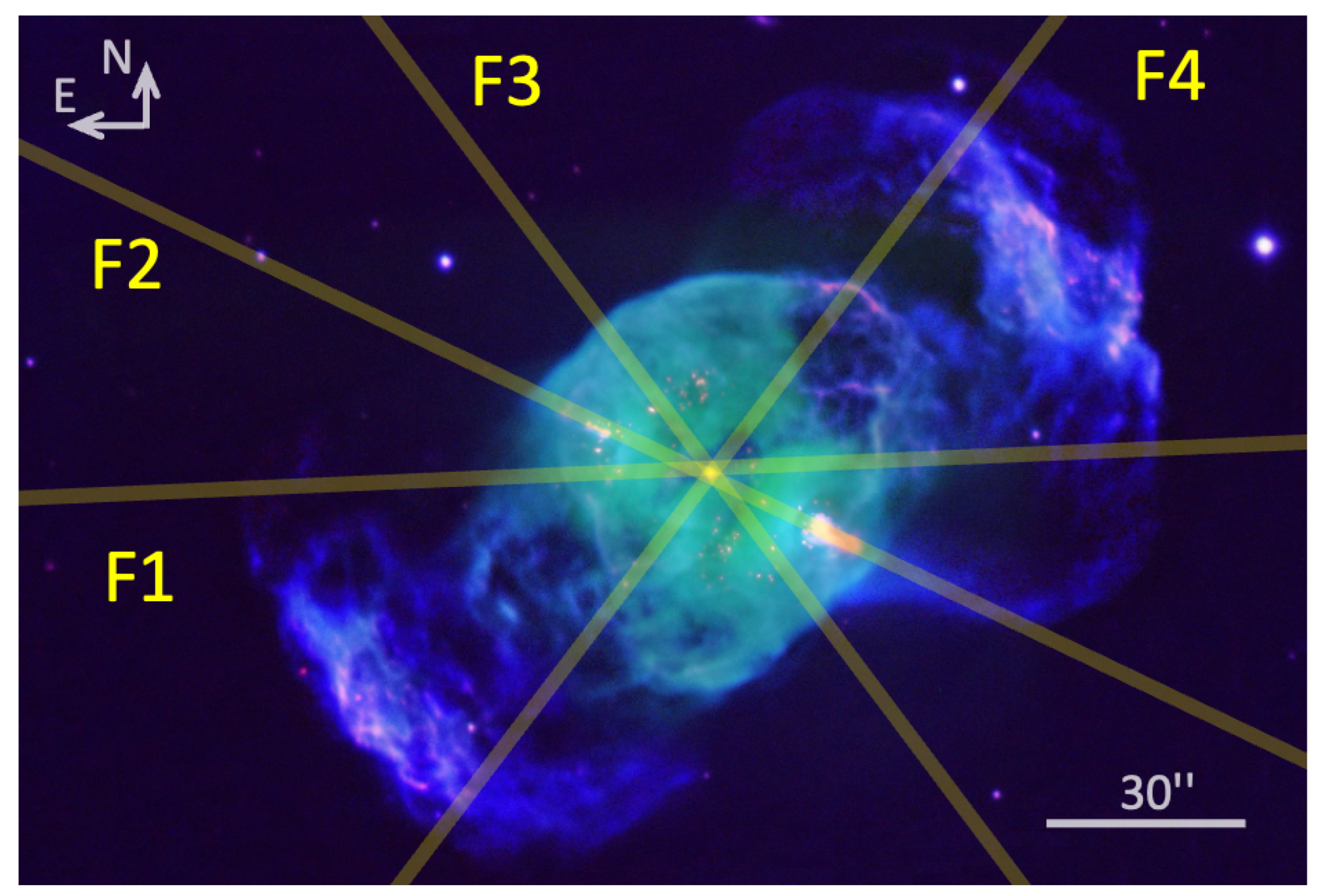
Figure 3.
Position-Velocity (PV) maps corresponding to the observed slit positions on NGC 2371, as labelled in Figure 2. The upper panels (slits F1, F3, and F4) display observations in [O iii]Å, while the lower panels (slits F2 and F3) depict observations in H and [N ii]Å. All maps are presented on a logarithmic scale. The zero position corresponds to the central star. The greyscale was chosen to improve the clarity of the image, and the velocity scale is relative to the systemic velocity.
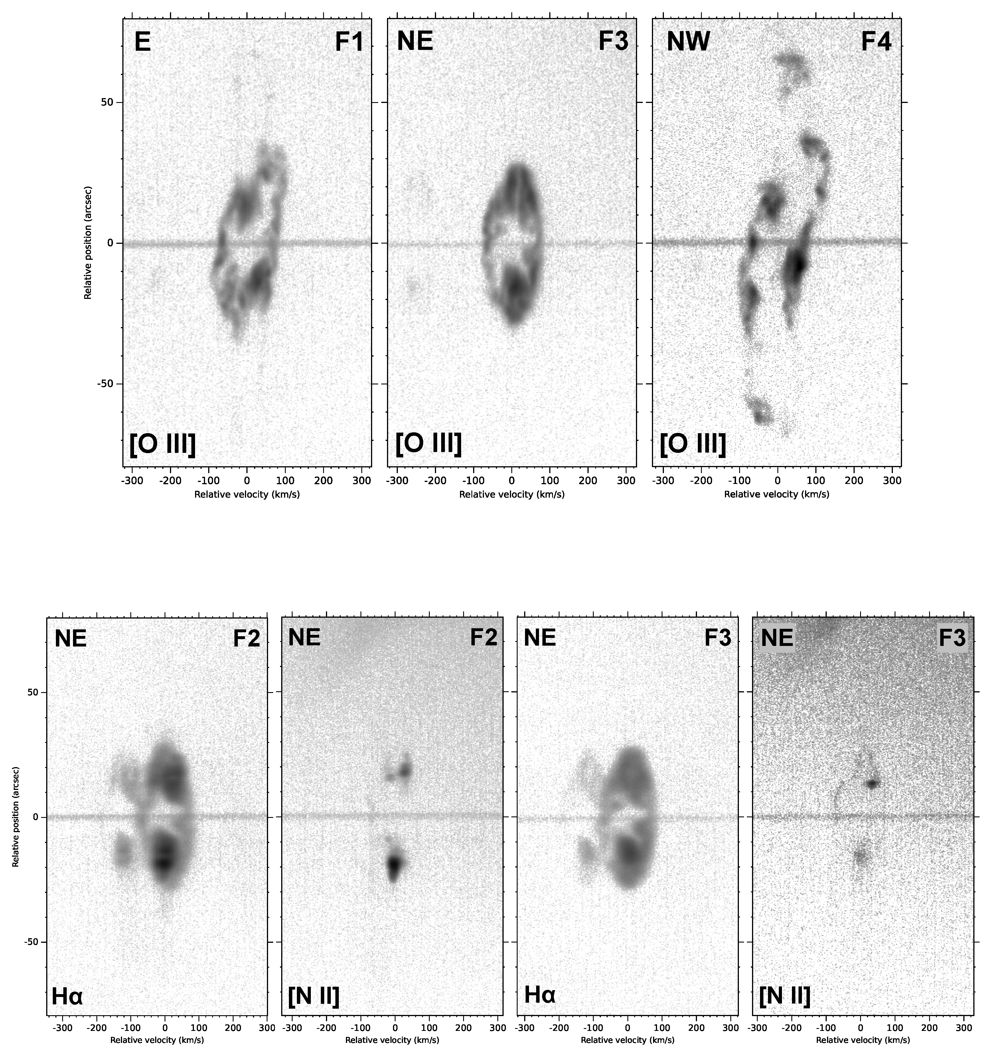
Figure 5.
Position-Velocity (PV) maps corresponding to the observed slit positions on NGC 2371, as labelled in Figure 4. All PV maps depict observations in [O iii]Å, utilising a logarithmic greyscale chosen to enhance image clarity. The velocity scale is relative to the systemic velocity.
Figure 5.
Position-Velocity (PV) maps corresponding to the observed slit positions on NGC 2371, as labelled in Figure 4. All PV maps depict observations in [O iii]Å, utilising a logarithmic greyscale chosen to enhance image clarity. The velocity scale is relative to the systemic velocity.
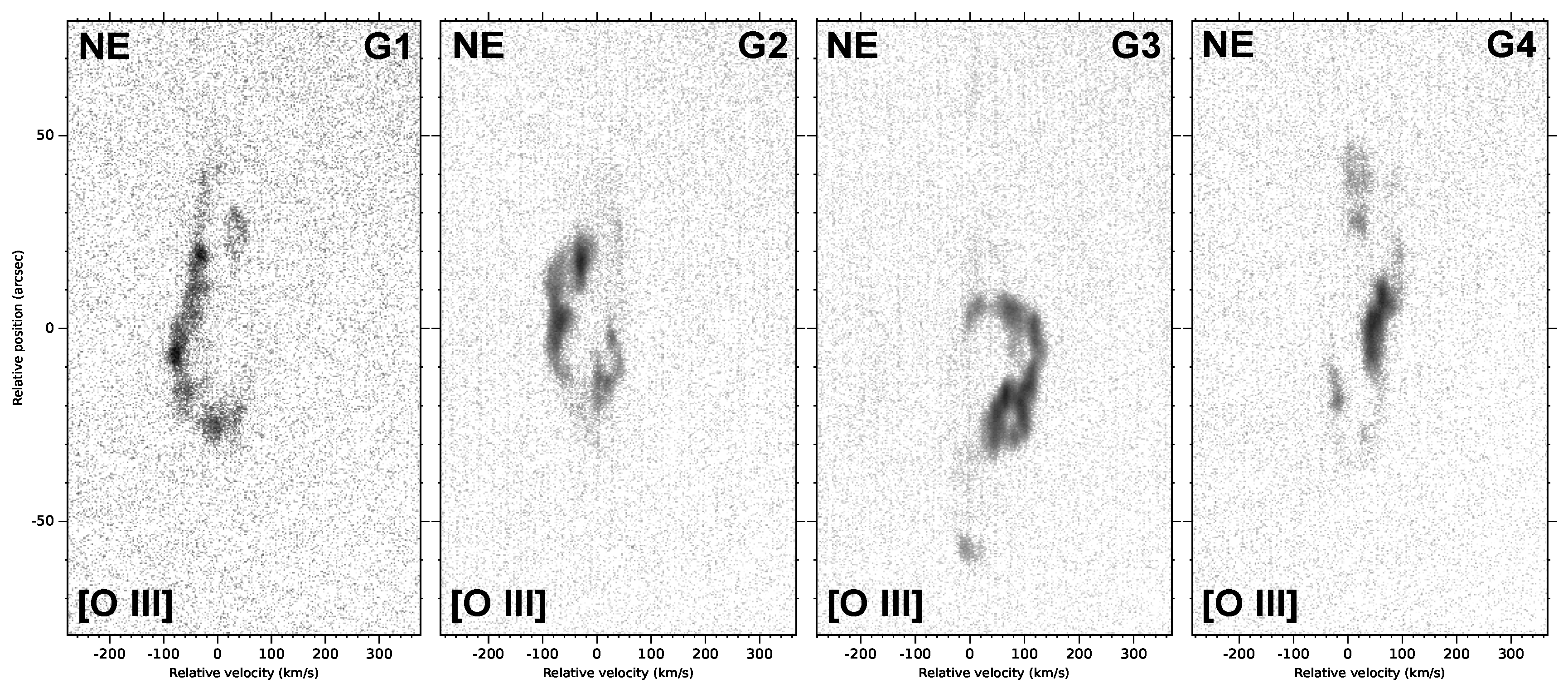
Figure 6.
Left: Components of the best ShapeX model for NGC 2371 that reproduce the SPM-MES observations. The barrel is in yellow, NW cap in red, SE cap in green, jets in red/orange, and the bipolar structure in blue/grey. Right Modelled structures superimposed on the direct image.
Figure 6.
Left: Components of the best ShapeX model for NGC 2371 that reproduce the SPM-MES observations. The barrel is in yellow, NW cap in red, SE cap in green, jets in red/orange, and the bipolar structure in blue/grey. Right Modelled structures superimposed on the direct image.
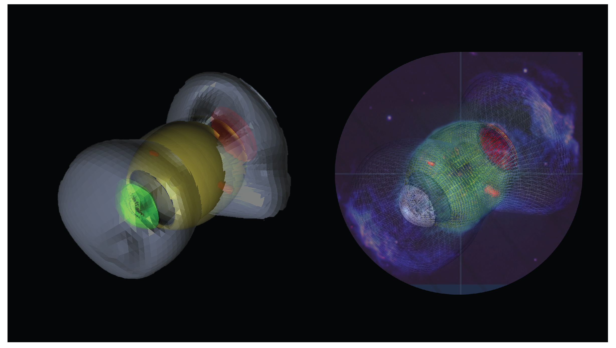
Figure 7.
Comparison between the observed and synthetic PV diagrams of NGC 2371. Top panels: slit positions F1–F4. Bottom panels: slit positions G1–G4. The greyscale background corresponds to the observed spectra, while the coloured contours represent the synthetic spectra from the final ShapeX model (the colour coding of the structures is the same as in Figure 6). Position angles (PAs) and emission lines are indicated in each panel. The velocity scale is defined with respect to the systemic velocity, whereas the spatial scale is centred on the central star for the F slits and on the geometrical centre of the emission for the G slits.


Table 1.
Details of the SPM-MES observations.
| Run | Date | Slit | PA | Filter | Exposure time (s) | Notesa |
|---|---|---|---|---|---|---|
| A | 2002 Jan 7 | A1 | 55° | [O iii] | 900 | 40″ to NW |
| A2 | 55° | [O iii] | 600 | CS | ||
| A3 | 55° | [O iii] | 900 | 60″ to SE | ||
| B | 2003 Feb 23 | B1 | 90° | [O iii] | 900 | 13″ to S |
| B2 | 90° | [O iii] | 900 | CS | ||
| B3 | 90° | [O iii] | 900 | 19″ to N | ||
| B4 | 90° | [O iii] | 900 | 30″ to N | ||
| B5 | 90° | [O iii] | 900 | 32″ to S | ||
| C | 2005 Feb 25 | C1 | ° | [O iii] | 1200 | CS |
| C2 | ° | [O iii] | 1200 | CS | ||
| D | 2005 Dec 13–14 | D1 | 66° | [O iii] | 900 | CS |
| D2 | 35° | [O iii] | 1800 | 33″ to NW | ||
| D3 | 35° | [O iii] | 1800 | 36″ to SE | ||
| E | 2009 Feb 4–6 | E1 | 66° | H+[N ii] | 1800 | Jets |
| E2_1 | ° | H+[N ii] | 900 | CS | ||
| E2_2 | ° | [O iii] | 900 | CS | ||
| E3 | ° | [O iii] | 900 | 17″ to NE | ||
| E4 | ° | [O iii] | 900 | 17″ to SW | ||
| F | 2016 Feb 20 | F1 | 93° | [O iii] | 1800 | CS |
| F2 | 65° | H+[N ii] | 1800 | CS | ||
| F3_1 | 37° | [O iii] | 1800 | CS | ||
| F3_2 | 37° | H+[N ii] | 1800 | CS | ||
| F4 | ° | [O iii] | 1800 | CS | ||
| G | 2016 Feb 21 | G1 | 37° | [O iii] | 1800 | 50″ to SE |
| G2 | 37° | [O iii] | 1800 | 28″ to SE | ||
| G3 | 37° | [O iii] | 1800 | 28″ to NW | ||
| G4 | 37° | [O iii] | 1800 | 50″ to NW |
a Slit positions are given either as CS when the slit crosses the central star, or as offsets (in arcsec, ″) from the CS toward the indicated direction.
Table 2.
Morphokinematical parameters of the proposed structures.
| Structure | PA | i | ||||||
|---|---|---|---|---|---|---|---|---|
| (arcsec) | (arcsec) | (°) | (°) | ( km s−1) | ( km s−1) | ( km s−1 arcsec−1) | (yrs) | |
| Lobes | n/a | n/a | 1.8 | |||||
| Barrel | n/a | 2.5 | ||||||
| NW cap | n/a | n/a | 5.0 | |||||
| SE cap | n/a | n/a | 3.0 | |||||
| E jet | n/a | n/a | 3.6 | |||||
| W jet | n/a | n/a | 1.0 |
a Truncated to this value; a full barrel size measures 37. b This structure is offset by from the barrel. c The position refers to the centre of the jet; its extent is . d Similar to (c), with an extent of .
Disclaimer/Publisher’s Note: The statements, opinions and data contained in all publications are solely those of the individual author(s) and contributor(s) and not of MDPI and/or the editor(s). MDPI and/or the editor(s) disclaim responsibility for any injury to people or property resulting from any ideas, methods, instructions or products referred to in the content. |
© 2025 by the authors. Licensee MDPI, Basel, Switzerland. This article is an open access article distributed under the terms and conditions of the Creative Commons Attribution (CC BY) license (http://creativecommons.org/licenses/by/4.0/).
Copyright: This open access article is published under a Creative Commons CC BY 4.0 license, which permit the free download, distribution, and reuse, provided that the author and preprint are cited in any reuse.


