
Submitted:
04 December 2025
Posted:
10 December 2025
You are already at the latest version
Abstract
Suppose $K_{_Y}$ and $K_{_X}$ are the image and the preimage of a nonlinear operator $\f:K_{_Y}\rightarrow K_{_X}$. It is supposed that the cardinality of each $K_{_Y}$ and $K_{_X}$ is $N$ and $N$ is large.
% large sets of observed and reference signals, respectively, each containing $N$ signals.
We provide an approximation to the map $\f$ that requires a prior information only on { a few elements} $p$ from
$K_{_Y}$, where $p\ll N$, but still effectively represents $\f(K_{_Y})$. It is
achieved under quite non-restrictive assumptions. The device behind the proposed method is based on a special
extension of the piecewise linear interpolation technique to the case of sets of stochastic elements.
The proposed technique provides {a single} operator that transforms any element from the {arbitrarily large } set $K_Y$. The operator is determined in terms of pseudo-inverse matrices so that it always exists.
Keywords:
approximation of nonlinear mappings
; error minimization
; optimization
; interpolation
1. Introduction
A purpose of the proposed methodology is to provide an effective way to transform large data sets. The methodology is motivated by the problems arising in signal processing where the nonlinear operator : is interpreted as a nonlinear system (or a nonlinear filter) transforming a set of stochastic signals to the set of stochastic signals . Therefore, below we refer to this terminology.
The device behind the proposed method is based on a special extension of the piecewise linear interpolation technique to the case of stochastic signal sets. The device is not straightforward and requires the careful substantiation presented in Section 2.3, Section 3.4, Section 4.2 and Section 4.4 below.
1.1. Motivations
The problem under consideration is motivated by the following observations.
1.1.1. Transformation of Large Sets of Signals
Suppose we need to transform a set of signals to another set of signals . The signals are represented by finite stochastic vectors1. A major associated difficulty and inconvenience which is common to many known filtering methodologies (see, for example, [1]–9,11,13,22,23,25]) is that they require a prior information on each reference signal to be estimated2. In particular, the filters in [22,23,25] are based on the use of either the reference signal itself, as in [22,23], or its estimate, as in [25]. The Wiener filtering approach (see, for example, [1]–13,23,25]) assumes that covariance matrices formed from a reference signal, , and an observed signal, , are known or can be estimated. The latter can be done, for instance, from samples of and . In particular, this means that the reference signal can be measured.
In the case of processing large signal sets, such restrictions become much more inconvenient.
The major motivating question for this work is as follows. Let : denote a filter that estimates a large set of reference signals, , from a large set of observed signals, . Each set contains N signals. Is it possible to construct a filter that requires a prior information only on few signals, p ≪ N, from KX but performs better than the known filters based on a prior information on every
reference signal from KX? We denote such a filter by (p−1).
It is shown in Section 2.3 and Section 4.4 that the positive answer is achievable under quite unrestrictive assumptions. The required features of filter are satisfied by its special structure described in Section 2.3, Section 3.1 and Section 3.4. The related conditions are also considered in those Sections.
1.1.2. Filtering Based on Idea of Piecewise Function Interpolation
The specific structure of the proposed filter follows from the extension of piecewise function interpolation [14]. This is because the technique of piecewise function interpolation [14] has significant advantages over the methods of linear and polynomial approximation used in known filtering techniques (such as, for example, those in [5,9]).
The structure of the proposed filter is presented in Section 2.3, Section 3.1 and Section 4.2 below.
1.1.3. Exploiting Pseudo-Inverse Matrices in the Filter Model
Most of the known filtering techniques, for example, those ones in [1]–3,6]–8,11,23,25], are based on exploiting inverse matrices in their mathematical models. In the cases of grossly corrupted signals or erroneous measurements those inverse matrices may not exist and, thus, those filters cannot be applied. The examples in Section 5 illustrate this case.
The filter proposed here avoids this drawback since its model is based on exploiting pseudo-inverse matrices. As a result, the proposed filter always exist. That is, it processes any kind of noisy signals. An extension of the filtering techniques to the case of implementation of the pseudo-inverse matrices is done on the basis of theory presented in [5].
1.1.4. Computational Work
Let m and n be the number of components of and of , respectively, where and each contains N signals. The known filtering techniques (e.g. see [1]–8,11,23,25]), applied to and , require computation of a product of an matrix and an matrix, as well as computation of an inverse or pseudo-inverse matrix for each pair of signals and . This requires and flops, respectively [26]. Thus, for the processing of all signals in and , the filters in [1]–8,11,23,25] require operations.
Alternatively, and can be represented by vectors, and , each with and components, respectively. In such a case, the techniques in [1]–8,11,23,25] can be applied to and as opposed to each signals in and . computational requirement is then and operations, respectively [26].
In both cases, but especially when N is large, computational work associated with the approaches [1]–8,11,23,25] becomes unreasonable hard.
For the filter to be introduced below, the associated computational work is substantially less. This is because requires computation of only p pseudo-inverse matrices associated with p selected signals in , where p is much less than the number of signals in . Therefore, for processing of the signal sets, and , requires only flops where . This comparison is illustrated in Section 5.
1.2. Relevant works
Some particular filtering techniques relevant to the method proposed below are as follows.
1.2.1. Generic Optimal Linear (GOL) Filter [5]
The generic optimal linear (GOL) filter in [5] is a generalization of the Wiener filter to the case when covariance matrix is not invertible and observable signal is arbitrarily noisy (i.e. when, in particular, noise is not necessarily additive and Gaussian). The GOL filter has been developed for processing an individual stochastic signal. Some ideas from [5] are used in the proof of Theorem 1 below.
1.2.2. Simplicial Canonical Piecewise Linear Filter [23]
A complex Wiener adaptive filter was developed in [23] from the two-dimensional complex-valued simplicial canonical piecewise linear filter [24]. The filter in [23] was developed for the processing of an individual stochastic signal and can be exploited when the reference signal is known and a ‘covariance-like’ matrix is invertible. The latter precludes an application to the signal types considered, for example, in Section 5: the matrices used in [23] are not invertible for the signals as those in Section 5. Similarly, the filters studied in [8,11] were developed for the processing of a single signal when the covariance matrices are invertible.
For the filter proposed here, these restrictions are removed.
1.2.3. Adaptive Piecewise Linear Filter [22]
1.2.4. Averaging Polynomial Filter [10,12]
The averaging polynomial filter proposed in [10,12] was developed for the purpose of processing infinite signal sets. The filter was based on an argument involving the ‘averaging’ over sets of signals under consideration. This device allows one to determine a single filter for the processing of infinite signal sets. At the same time, it leads to an increase in the associated error when signals differ considerably from each other. This effect is illustrated in Section 5 below.
1.2.5. Other Relevant Filters
The technique developed in [13] is an extension of the GOL filter to the constraint problem with respect to the filter rank. It concerns data compression.
The methods in [6,7,15,16] have been developed for deterministic signals. Motivated by the results achieved in [15,16], adaptive filters were elaborated in [17]. A theoretical basis for the device proposed in [15,16] is provided in [18].
We note that the idea of piecewise linear filtering has been used in the literature in several very different conceptual frameworks, despite exploiting some very similar terms (as in [15]–24]). At the same time, a common feature of those techniques is that they were developed for the processing of a single signal, not of large signal sets as in this paper. In particular, piecewise linear filters in [19] have been obtained by arranging linear filters and thresholds in a tree structure. Piecewise linear filters discussed in [20] were developed using so-called threshold decomposition, which is a segmentation operator exploited to split a signal into a set of multilevel components. Filter design methods for piecewise linear systems proposed in [21] were based on a piecewise Lyapunov function.
1.3. Difficulties Associated with the Known Filtering Techniques
Basic difficulties associated with applying the known filtering techniques to the case under consideration (i.e. to processing of large signal sets, and ) are that:
(i) they require an information on each reference signal (in the form of a sample, for example),
(ii) matrices used in the known filters can be not invertible (as in the simulations considered below in Section 5) and then the filter does not exist, and
(ii) the associated computation work may require a very long time. For example, in simulations (Section 5), MATLAB was out of memory for computing the GOL filter [5] when each of sets and was represented by a long vector (this option has been discussed in Section 1.1.4 above).
1.4. Differences from the Known Filtering Techniques
The differences from the known filtering techniques discussed above are as follows.
(i) We consider a single filter that processes arbitrarily large input-output sets of stochastic signal-vectors. The known filters [1]–9,11,13,15]–25] have been developed for the processing of an individual signal-vector only. In the case of their application to arbitrarily large signal sets, they imply difficulties described in Section 1.1 and Section 1.3 above.
(ii) As a result, our piecewise linear filter model (Section 3), the statement of the problem (Section 3.3 below) and consequently, the device of its solution (Section 4 below) are different from those considered in [15]–24]. In this regard, see also Section 1.2.5.
(iii) The above naturally leads to a new structure of the filter (presented in Section 3.4 and Section 4.2 below) which is very different from the known ones.
1.5. Contribution
In general, for the processing of large data sets, the proposed filter allows us to achieve better results in comparison with the known techniques in [1]–25]. In particular, it allows us to
(i) achieve a desired accuracy in signal estimation3,
(ii) exploit a prior information only on few reference signals, p, from the set that contains signals or even infinite number of signals,
(iii) find a single filter to process any signal from the arbitrarily large signal set,
(vi) determine the filter in terms of pseudo-inverse matrices so that the filter always exists, and
(v) decrease the computational load compared to the related known techniques.
2. Some Preliminaries
2.1. Notation
The signal sets we consider are, in fact, special representations of time series.
Let be a probability space4, and and be arbitrarily large sets of signals such that
where We interpret as a reference signal and as an observable signal, an input to the filter studied below5. The variable represents time6. Then, for example, the stochastic signal x(t, ·) can be interpreted as an arbitrary stationary time series.
Let be a sequence of fixed time-points such that
Because of the partition (1), the sets and are divided in `smaller’ subsets and , respectively, so that, for each ,
Therefore, and can now be represented as
2.2. Brief Description of the Problem
Given two arbitrarily large sets of stochastic signals, and , find a single filter : that estimates the signal with a controlled, associated error. Note that in our formulation the set can be finite or infinite.
2.3. Brief description of the method
The solution of the above problem is based on the representation of the proposed filter in the form of a sum with terms where each term, j, is interpreted as a particular sub-filter (see (4) and (5) below). Such a filter is denoted by .
The sub-filter j transforms signals that belong to ‘piece’ of set to signals in ‘piece’ of , i.e. . Each sub-filter j depends on two parameters, and .
The prime idea is to determine j (i.e. and ) separately, for each . The required and follow from the solutions of the equation (11) and an associated minimization problem (11) (see Section 3.4 and Section 4.2 below). This procedure adjusts j so that the error associated with the estimation of is minimal.
A motivation for such a structure of the filter is as follows. The method of determining and provides an estimate that interpolates at and . In other words, the filter is flexible to variations in the sets of observed and reference signals and , respectively. Due to this way of determining j, it is natural to expect that the processing of a ‘smaller’ signal set, , may lead to a smaller associated error than that for the processing of the whole set by a filter which is not specifically adjusted to each particular piece .
As a result, represents a special piecewise interpolation procedure and, thus, should be attributed with the associated advantages such as, for example, the high accuracy of estimation.
In Section 4.4, this observation is confirmed. In Section 2 and Section 5, it is also shown that the proposed technique allows us to avoid the difficulties discussed in Section 1.3 above.
3. Description of the Problem
3.1. Piecewise Linear Filter Model
Let be a filter such that, for each ,
where
Thus, j is defined by an operator such that
3.2. Assumptions
In the known approaches related to filtering of stochastic signals (e.g. see [1]–13,23,25]), it is assumed that covariance matrices formed from the reference signal and observed signal are known or can be estimated.
The assumption used here is similar. The covariance matrices that are assumed to be known or can be estimated, are formed from selected signal pairs with and p to be a small number8, , where N is the number of signals in or .
3.3. The Problem
In (4)-(6), parameters of the filter , i.e. vector and matrix , for , are unknown. Therefore, under the assumptions described in Section 3.2, the problem is to determine and , for . The related problem is to estimate an error associated with the filter .
Solutions to the both problems are given in Section 4.2 and Section 4.4, respectively. In particular, in the following Section 3.4, interpolation conditions (8) and (11) are introduced that lead to a determination of and .
3.4. Interpolation Conditions
Let us denote
where is the Euclidean norm of .
For , let be an estimate of determined by known methods [1]–13,23,25]. This is the initial condition of the proposed technique.
Sub-filter 1: For , and solve
respectively. Then an estimate of , , for , is determined as
where and satisfy (8). In particular, and
Extending this procedure up to , where , we set the following. Let be an estimate of defined by the preceding steps as
Then sub-filter is defined as follows.
Sub-filter : For , and solve
respectively. Then an estimate of , , for , is determined as
4. Main Results
4.1. General Device
In accordance withe the scheme presented in Section 3.1 and Section 3.4 above, an estimate of the reference signal , for any , by the piecewise linear interpolation filter , is given by
where, for each the sub-filter j is given by (5), and is defined from the interpolation conditions (8) and (11).
4.2. Determination of Piecewise Linear Interpolation Filter
Let us denote
We need to represent and in terms of their components as follows:
where and are stochastic variables, for all .
Then we can introduce the covariance matrix
where
Below, is the Moor-Penrose generalized inverse of a matrix M.
Now, we are in a position to establish the main results.
Theorem 1.
Let
be sets of reference signals and observed signals, respectively. Let , for , be such that
For let be a known estimate of 9. Then, for any , the proposed piecewise linear interpolation filter transforming any signal to an estimate of , , is given by
where
and where In is n × n identity matrix and MBj is an m × n arbitrary matrix.
Proof: The proof of Theorem 1 is given in Section A.
It is worthwhile to observe that, due to an arbitrary matrix in (19), the filter is not unique. In particular, can be chosen as the zero matrix similarly to the generic optimal linear [5] (which is also not unique by the same reason).
4.3. Numerical Realization of Filter and Associated Algorithm
4.3.1. Numerical Realization
In practice, the set (see Section 2.1) is represented by a finite set , i.e. where .
For , the estimate of , , and observed signal are represented by and matrices
The sequence of fixed time-points introduced in (1) is such that
where and where and are positive integers such that .
For , vectors and associated with in (21) are represented, respectively, by
4.3.2. Algorithm
As it has been mentioned in Section 3.4, it is supposed that, for an estimate of , , is known and can be determined by the known methods. This is the initial condition of the proposed technique.
On the basis of the results obtained in Section 3.4 and Section 4.2, the performance algorithm of the proposed filter consists of the following steps. For , we write .
(Possible ways to get estimates of and are discussed below in Section 4.5.)
Final parameters:, ,…, .
Algorithm:
• for to p do
begin
• for to do
begin
end
end
4.4. Error Analysis
It is natural to expect that the error associated with the piecewise interpolating filter decreases when decreases. Below, in Theorem 3, we justify that this observation is true. To this end, first, in the following Theorem 2, we establish an estimate of the error associated with the filter F.
Let us introduce the norm by
We also denote .
Let us suppose that and are Lipschitz continuous signals, i.e. that there exist real non-negative constants and , with , such that, for ,
where .
Theorem 2.
Under the conditions (23) the error associated with the piecewise interpolation filter, , is estimated as follows:
Proof: The proof of Theorem 2 is given in Section A. □
Further, to show that the error of the reference signal estimate tends to the zero, we need to assume that, for , the known estimate differs from for the value of the order , i.e. that, for some constant ,
Theorem 3.
Let the conditions (23) and (25) be true. Then the error associated with the piecewise interpolating filter F, , decreases in the following sense:
Proof: The proof of Theorem 3 is given in Section A. □
Remark 1.
We would like to emphasize that the statement of Theorem 3 is fulfilled only under assumptions (23) and (25). At the same time, the assumptions (23) and (25) are not restrictive from a practical point of view. The condition (23) is true for Lipschitz continuous signals and , i.e. for very wide class of signals. The condition (25) is achieved by a choosing an appropriate known method (e.g. see [1]–13,23,25]) to find the estimate used in the proposed filter (see (8) and Theorem 1).
4.5. Some Remarks Related to the Assumptions of the Method
As it has been mentioned in Section 3.2, for , matrices and in (19) are assumed to be known or can be estimated. Here, p is a chosen number of selected interpolation signal pairs (see Section 3.4). We note that normally p is much smaller than the number of input-output signals and . Therefore, to estimate any signal from an arbitrarily large set , only a small number, p, of matrices and should be estimated (or be known). This issue has also been discussed in Section 1.1.1 and Section 1.1.4.
By the proposed method, is estimated for . While in (19) can be directly estimated from observed signals and , an estimate of matrix depends on the reference signal (see (14) and (15)) which is unknown (because the estimate is considered for ).
Some possible approaches to an estimation of matrix could be as follows.
1. In the general case, when and are arbitrary signals as discussed in Section 2.1 above, matrix can be estimated as proposed, for example, in [27], from samples of and .
3. Let be a matrix obtained from matrix where the term is replaced by with . Since with is known, matrix can be considered as an estimate of .
4. In the important case of an additive noise, can be represented in the explicit form. Indeed, if
where is a random noise, then and matrix can be represented as follows:
We note that the RHS of (27) depends only on observed signals , , estimated signal , and noise , not on the reference signal . In particular, in (27), the term can be estimated as where . It is motivated by the Holder’s inequality for integrals. The second term in (27), , can be estimated from the samples of and .
We also note that the first term in the RHS of (27), , is similar to the related covariance matrix in the Wiener filtering approach [5].
5. Other known ways to estimate can be found in [5], Section 5.3.
5. Simulations
5.1. General Consideration
In these simulations, in accordance with Section 4.3.1, signal sets and (see Section 2.1) are given by
where, for , and . In many practical problems (arising, for example, in a DNA analysis the number N is quite large, for instance, .
We set and . Thus, in these simulations, the interval (see Section 2.1 and Section 4.3.1) is modelled as 141 points with so that .
The sequence of fixed time-points in (1) is now such that
Below, in Examples 1-12, four particular choices of the specific interpolation signal pairs (introduced in Section 3.4) are considered, for and 28. Points are as follows.
For , if , then , respectively, where and .
For , if , then , and if , then , where .
Signals and have been simulated as digital images represented by matrices
respectively, for , so that represents an image that should be estimated from an observed image . A column of matrices and , and , for , represents a realization of signals and , respectively.
Note that did not used in the piecewise linear filter below since they are not supposed to be known. They are represented here for illustration purposes only. In particular, are used to compare their estimates by different filters.
Observed noisy signals have been simulated in different forms presented by (40), (49), (50) and (51) in the Examples 1-12 below. We note that the considered observed signals are grossly corrupted.
To estimate the signals , ..., from the observed signals , ..., , the proposed piecewise linear filter , the generic optimal linear (GOL) filters [5] and the averaging polynomial filter [12] have been used.
The filters proposed in [12,13,22,23] have not been applied here by the reasons discussed in Section 1. In particular, the filter in [23] cannot be applied to signals represented by , ..., in the form (40), (49), (50) and (51) below because the associated inverse matrices used in [23] do not exist.
For signals under consideration (given by matrices and with ), the filter , the generic optimal linear (GOL) filters [5] and the averaging polynomial filter [10,12] are represented as follows.
(i) Piecewise linear filter .For , designates an interpolation pair defined similarly to that in Section 3.4. Each and is associated with in (25) so that
The estimate of by the filter is given by
and where and are estimates of matrices and in (19), respectively. In particular, can be represented in the form
Further, matrix depends on where is unknown. Therefore a determination of is reduced, in fact, to finding an estimate of . Since it is customary to find in terms of signal samples [5], has been presented as
and has been constructed from a sample of as follows. The sample of is a matrix presented by odd columns of . Then an estimate of is chosen as a matrix where each odd column is a related odd column of , and each even column is an average of two adjacent columns. The last column in is the same as its preceding column.
This way of estimating was chosen for illustration purposes only. Other related methods have been considered in Section 4.5.
The errors associated with the filter are given by
(ii) Generic optimal linear (GOL) filters [5]. To each signal , an individual GOL filter has also been applied, so that estimates from in the form
for each . Thus, the GOL filter requires an estimate of 141 matrices , for each .
Similarly to matrix in the filter above, the matrix has been estimated from samples of each , , for each .
One of the advantages of the proposed filter is that requires a smaller number, p, of samples of , , to be known (where ).
The errors associated with filters are given by
(iii) Averaging polynomial filters [10,12]. By the methodology in [10], the averaging polynomial filter W is based on the use of the estimates of the covariance matrices, and , in the form
Then, for each, , the estimate of is given by
The errors associated with the filter W are given by
5.2. Simulations with Signals Modelled from Images ‘Plant’: Application of Piecewise Interpolation Filter and GOL Filters
Here, results of simulations for reference signals represented by matrices (see (29) above) formed from images ‘plant’10 are considered. Typical selected images are shown in Figure 9.
Observed noisy images have been simulated in the form
for each Here, • means the Hadamard product, and and are matrices with random entries. The entries of are normally distributed with mean zero, variance one and standard deviation one. The entries of are uniformly distributed in the interval . A typical example of such images is given in Figure 10 (a).
To demonstrate the effectiveness of the proposed filter , sub-filters and associated interpolation signal pairs have been chosen in four different ways as follows.
Example 1. First, for , the interpolation signal pairs are
The error values associated with filter are evaluated by (37). The graph of is presented in Figure 11 (a).
Example 2. For , the interpolation signal pairs are
The error magnitudes associated with the piecewise interpolation filter constructed by (31)-(36) with the interpolation signal pairs given by (43)-(44) are diagrammatically shown in Figure 11 (b).
It follows from Figure 11 (b) that the errors associated with filter is less than those of filter . This is a confirmation of Theorem 3.
Example 3. Further, for , the interpolation pairs are
In Figure 11 (c), the errors associated with the piecewise interpolation filter are presented. The Figure 11 (c) demonstrates a further confirmation of Theorem 3: the errors associated with the piecewise interpolation filter diminishes as p increases.
Example 4. Finally, the number of interpolation signal pairs is so that
In this case, when p is grater than in the previous Examples 1-3, the errors associated with the piecewise interpolation filter are smaller than those associated with filters , and - see Figure 11 (d).
The diagrams of errors associated with the GOL filters [5] are also presented in Figure 11. It follows from Figure 11 that proposed filters , , and provide the better accuracy then that of the GOL filters.
At the same time, the filter is easer to implement since it requires less initial information compared to GOL filters, as it has been discussed in Section 1.1.1 and Section 1.1.4.
Results of the application of the averaging polynomial filter [10,12] are discussed in Section 5.4 below.
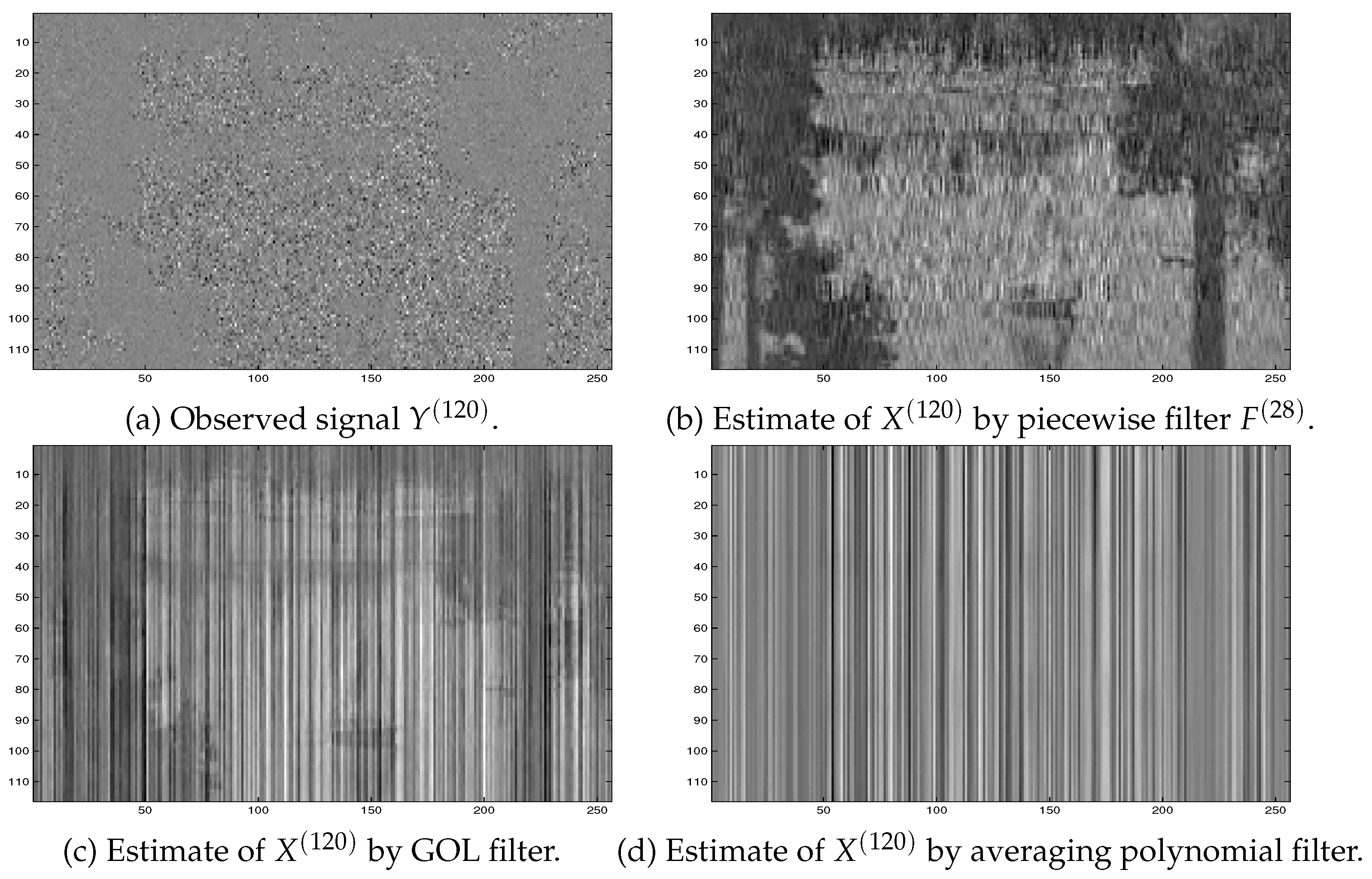
5.3. Simulations with Signals Modelled from Images ‘Boat’: Application of Piecewise Interpolation Filter and GOL Filters
In this section, results of the simulations for a different type of signals than those considered in Section 5.2 above are presented. Here, the reference signals are formed from images ‘boat’11.
Observed noisy signals have been simulated in the form
for each The noise term is different from that in (40).
As in Section 5.2, the piecewise interpolation filter is constructed by (31)-(36). In Examples 5-8 below, the number of sub-filters and associated interpolation signal pairs have been chosen in four different ways.
Example 5. First, similar to Example 1, the number of interpolation signal pairs has been chosen as , and and have been presented as in (41)-(42).
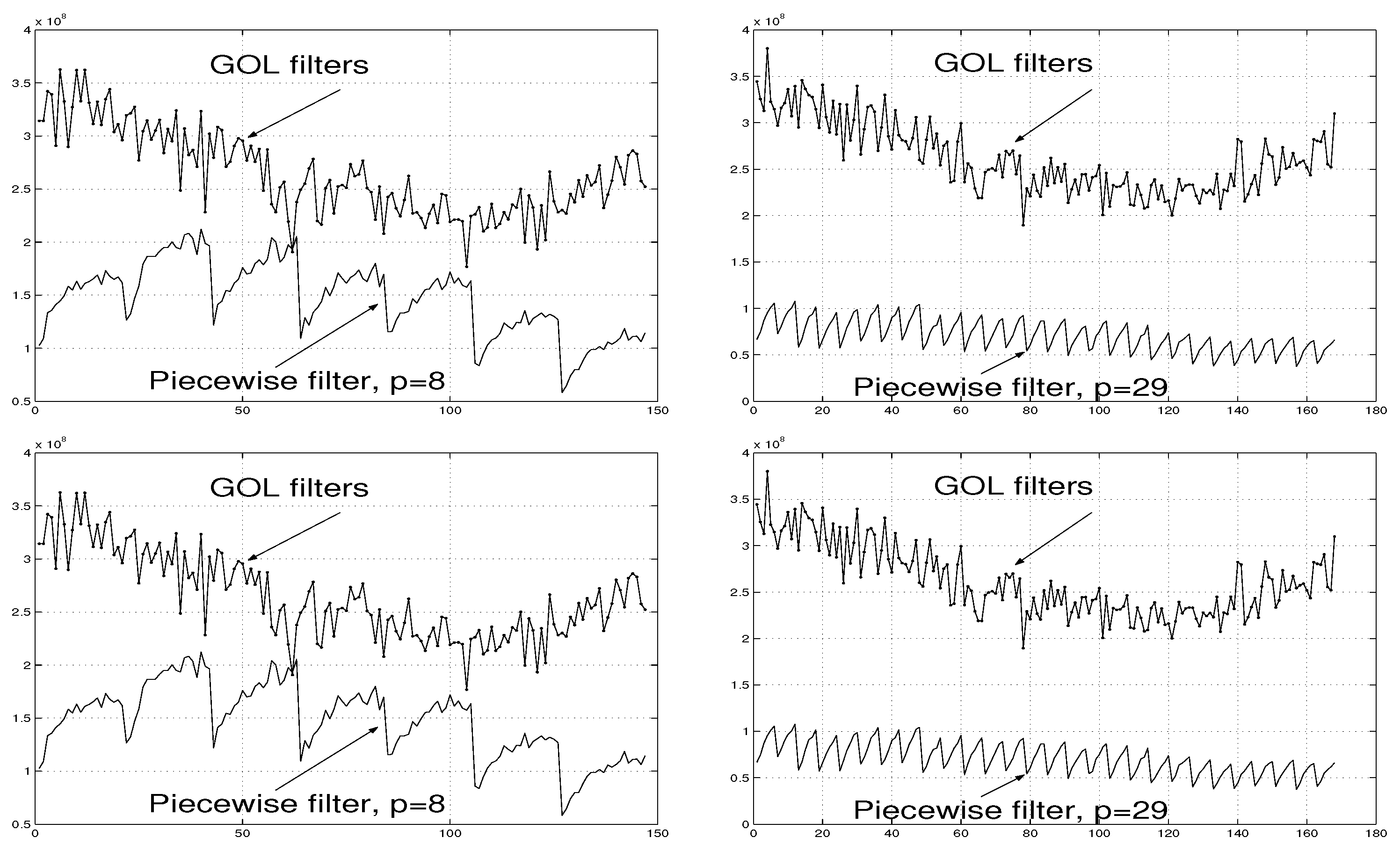
The error values associated with the piecewise interpolation filter applied to these data are presented in Figure 14 (a).
Example 6. For the grater number of interpolation signal pairs than that in Example 5, , and for and () chosen as in (43)-(44), the error magnitudes associated with the piecewise interpolation filter are diagrammatically shown in Figure 14 (b). A comparison between Figure 14 (a) and (b) demonstrates that the increase in p implies the decrease in the errors associated with the filter .
Example 7. For , and for and () chosen as in (45)-(46), the errors associated with the piecewise interpolation filter are further less than those for filters and . See Figure 14 (c) in this regard.
Example 8. The further increase in p to , confirms this tendency. The piecewise interpolation filter with and () chosen similar to (47)-(48) produces the associated errors represented in Figure 14 (d). They are, clearly, less than the errors associated with filters , and .
The errors associated with the GOL filters are also presented in Figure 14 (a)-(d). The figures clearly demonstrate the advantage of the piecewise interpolation filter .
Results of the application of the averaging polynomial filter [12] are discussed in Section 5.4 below.
5.4. Results of Simulations for Averaging Polynomial Filter [10,12]
To further illustrate the effectiveness of the proposed piecewise interpolation filter, in this Section, results of simulations for the averaging polynomial filter [10,12] are presented. The filter has been applied to two different types of data considered in Section 5.2 and Section 5.3.
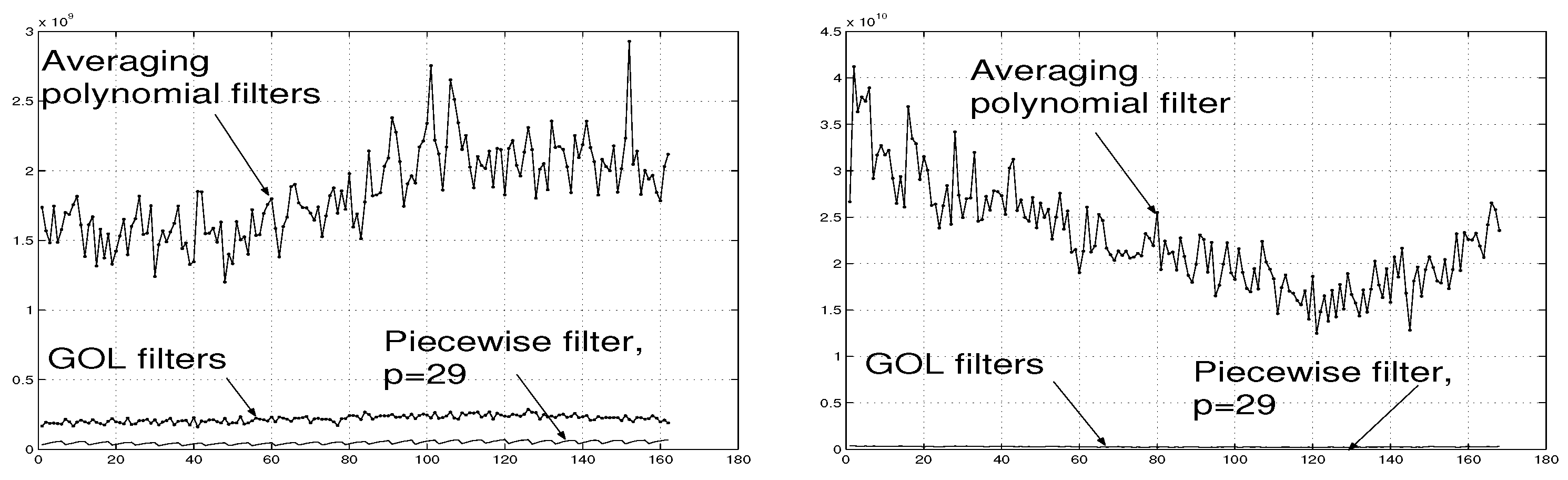
Example 9. The filter [10,12] applied to signals considered in Section 5.2 gives the associated errors (see (39)) represented in Figure 15 (a). For a comparison, the errors associated with the piecewise interpolation filter and the GOL filters [5] are also given in Figure 15 (a).
A typical example of the estimated signal by the averaging polynomial filter [10,12] is presented in Figure 10 (d) above.
Example 10. The averaging polynomial filter [12] applied to signals considered in Section 5.3 produces the associated errors shown in Figure 15 (b). The errors associated with the piecewise interpolation filter are much smaller and they are not discerned in Figure 15 (b).
Together with Figure 10, Figure 11, Figure 13 and Figure 14, Figure 15 (a) and (b) illustrate the advantage of the piecewise interpolation filter.
Figure 1.
Examples of selected signals to be estimated from observed data.
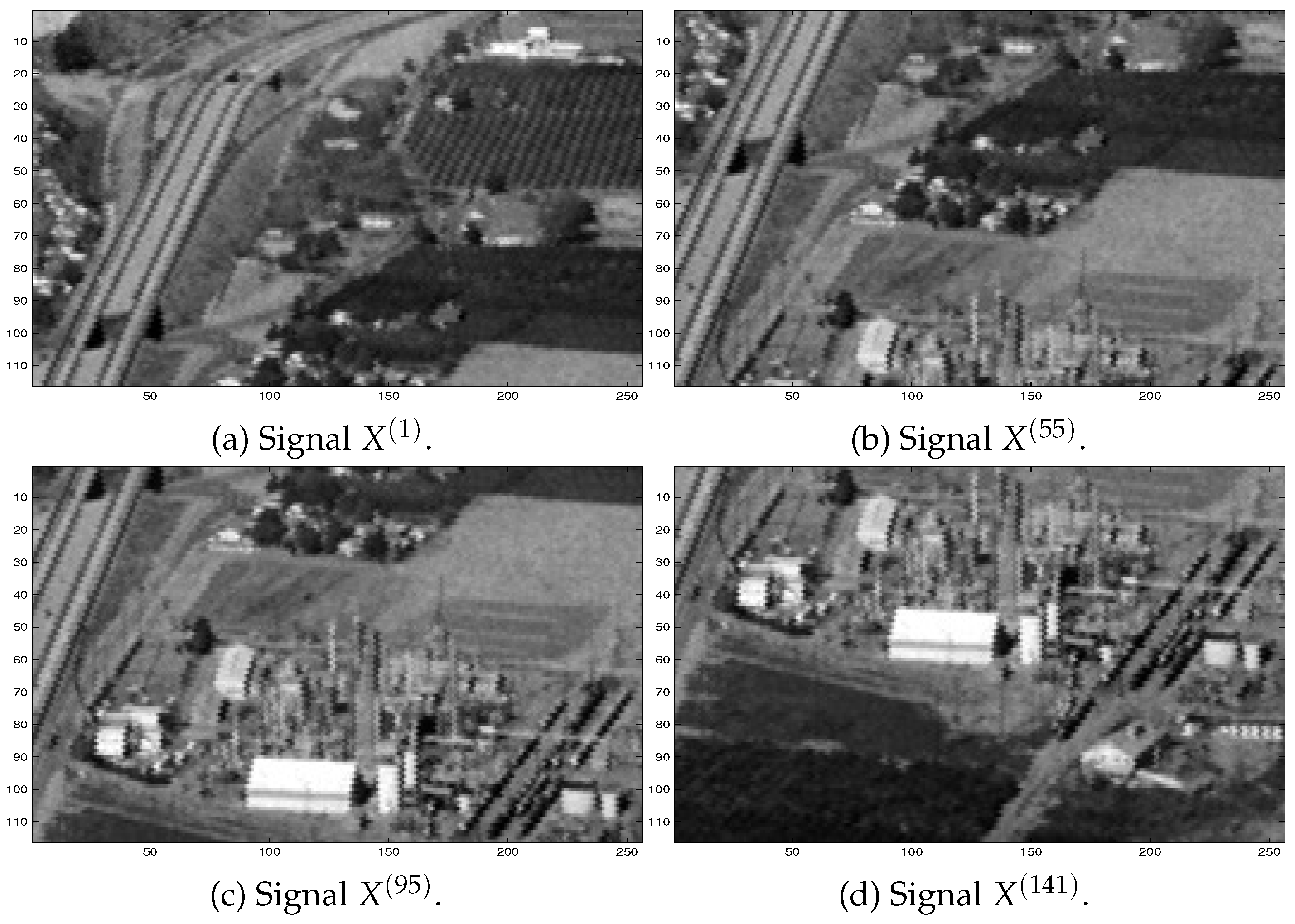
Figure 2.
Examples of the observed signal and the estimates obtained by different filters.
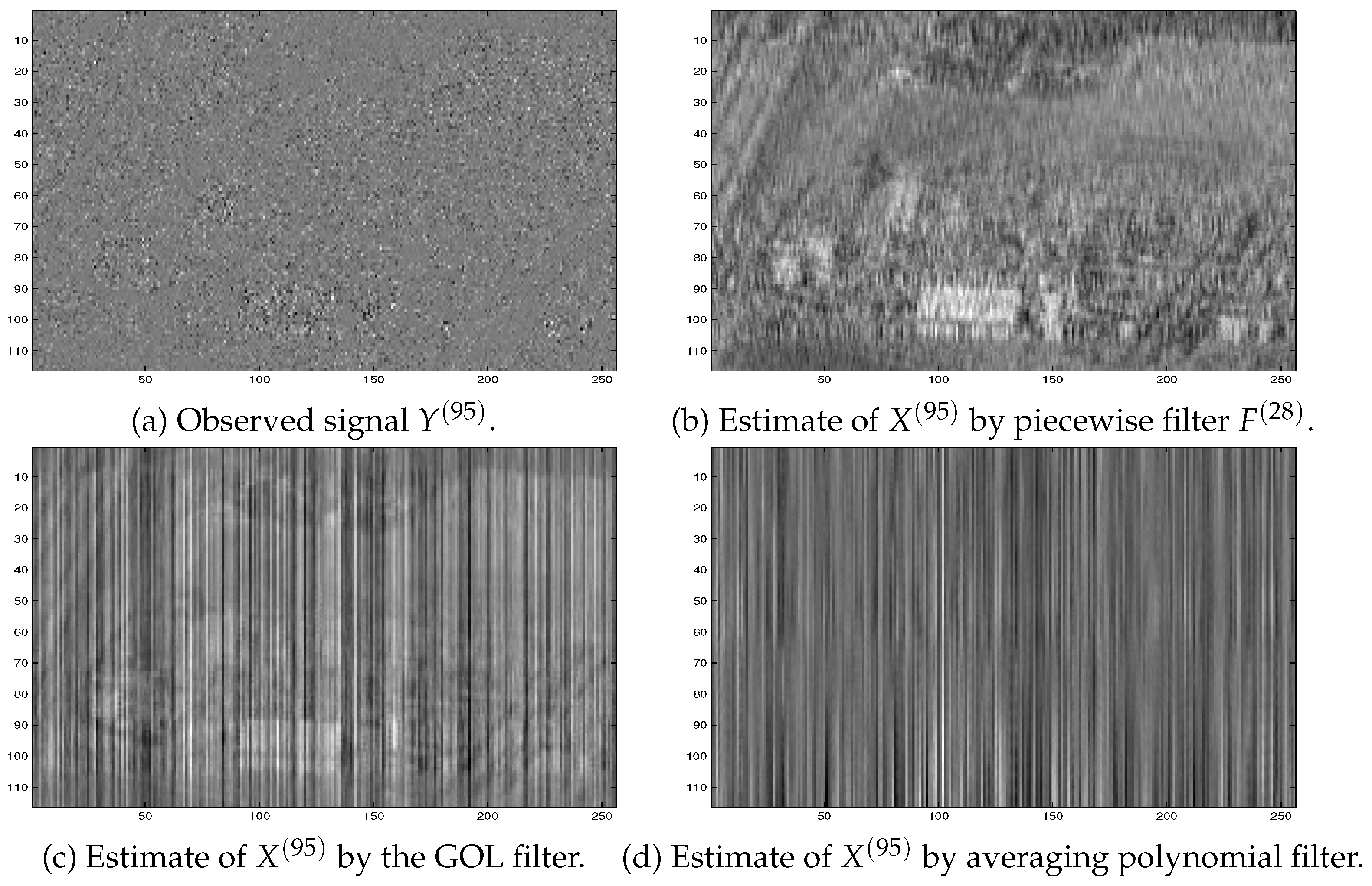
Figure 3.
Illustration of the errors associated with the piecewise interpolation filters and the GOL filters [5] applied to signals described in Examples 1–4.
Figure 3.
Illustration of the errors associated with the piecewise interpolation filters and the GOL filters [5] applied to signals described in Examples 1–4.

Figure 4.
Examples of selected signals to be estimated from observed data considered in Example 5-9.
Figure 4.
Examples of selected signals to be estimated from observed data considered in Example 5-9.
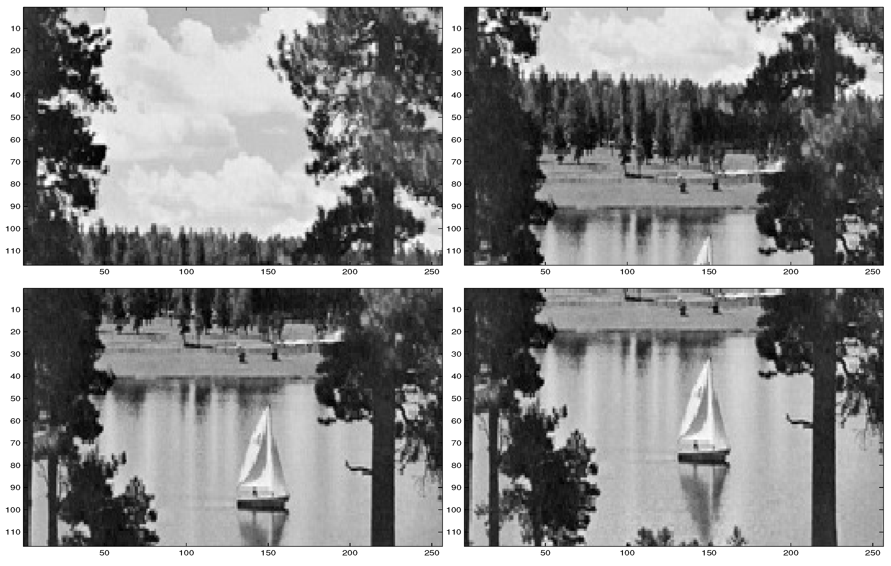
Figure 5.
Examples of the observed signal and the estimates obtained by different filters.
5.5. Further Simulations with Different Type of Noise
In Examples 11 and 12 below, a different type of noise is considered. Unlike the multiplicative noise in (40) and (49), here, the noise is additive.
Example 11. First, the piecewise interpolation filter , the GOL filters [5] and the averaging polynomial filter [12] have been applied to the observed signals given by
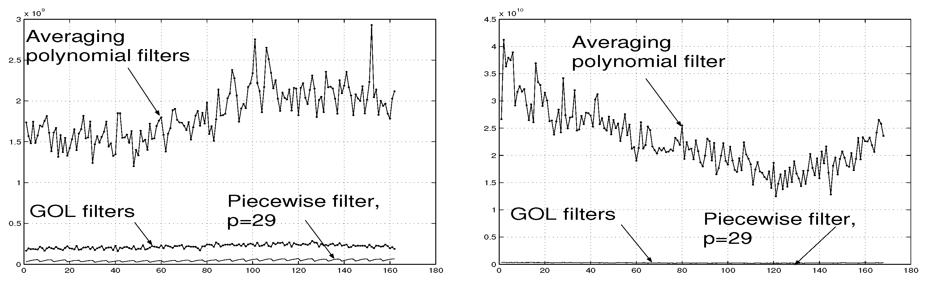
where is as in Section 5.2, i.e. is formed from the images ‘plant’. In Figure 8 (a), the diagrams of the errors associated with filter and the GOL filters [5] are given. The errors associated with the averaging polynomial filter [12], , are much grater (of order ) and they are not presented in Figure 8 (a).
Figure 6.
Illustration of errors associated with the piecewise interpolation filter of order p and the generic optimal linear (GOL) filters [5] applied to signals described in Examples 5–8.
Figure 6.
Illustration of errors associated with the piecewise interpolation filter of order p and the generic optimal linear (GOL) filters [5] applied to signals described in Examples 5–8.
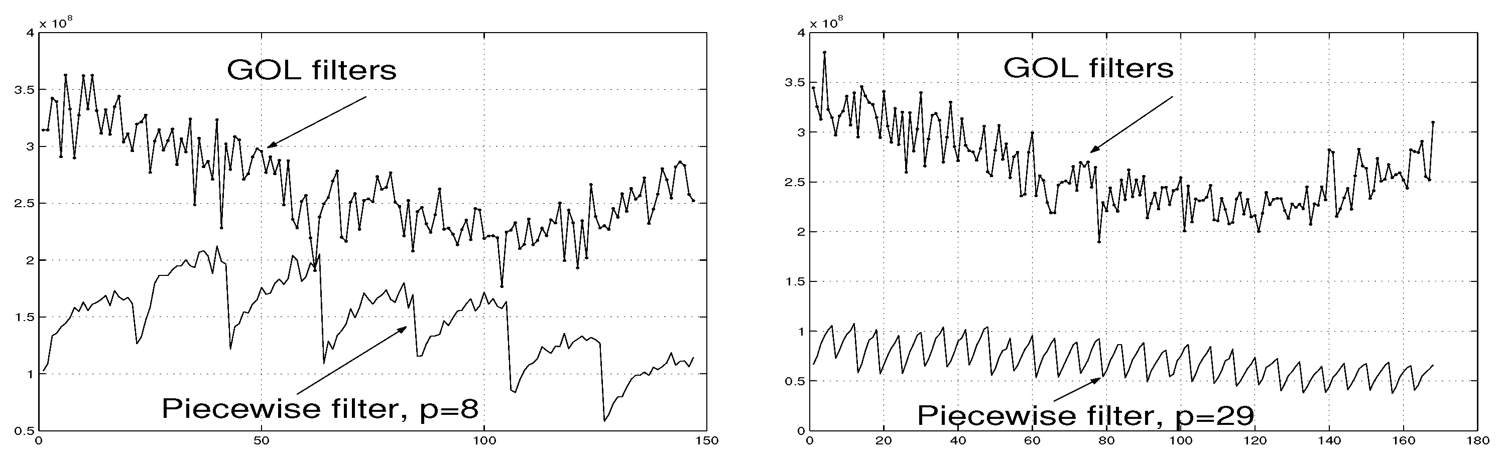
Figure 7.
Illustration of errors associated with the averaging polynomial filters [10,12] in Examples 9 and 10.
Example 12. In this example, the reference signals are as those in Section 5.3, i.e. they are formed from the image ‘boat’. The observed signals are given by
The piecewise interpolation filter and the GOL filters [5] estimate the reference signals with the associated errors represented in Figure 8 (b). As in Example 11 above, in this case, the errors associated with the averaging polynomial filter [10,12] are much grater (of order ) and they are not presented in Figure 8 (b).
Examples 11 and 12 further demonstrate the advantages of the proposed piecewise interpolation filter.
Figure 8.
Illustration of errors associated with the piecewise interpolation filter and the generic optimal linear (GOL) filters [5] applied to signals described in Examples 11 and 12.
Figure 8.
Illustration of errors associated with the piecewise interpolation filter and the generic optimal linear (GOL) filters [5] applied to signals described in Examples 11 and 12.
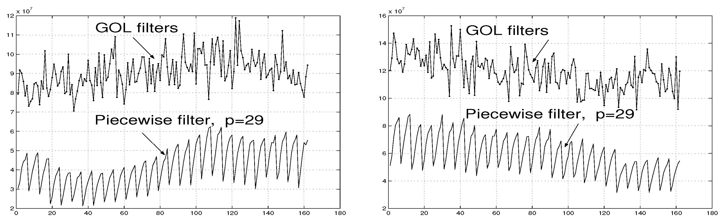
Figure 9.
Examples of selected signals to be estimated from observed data.

Figure 10.
Examples of the observed signal and the estimates obtained by different filters.
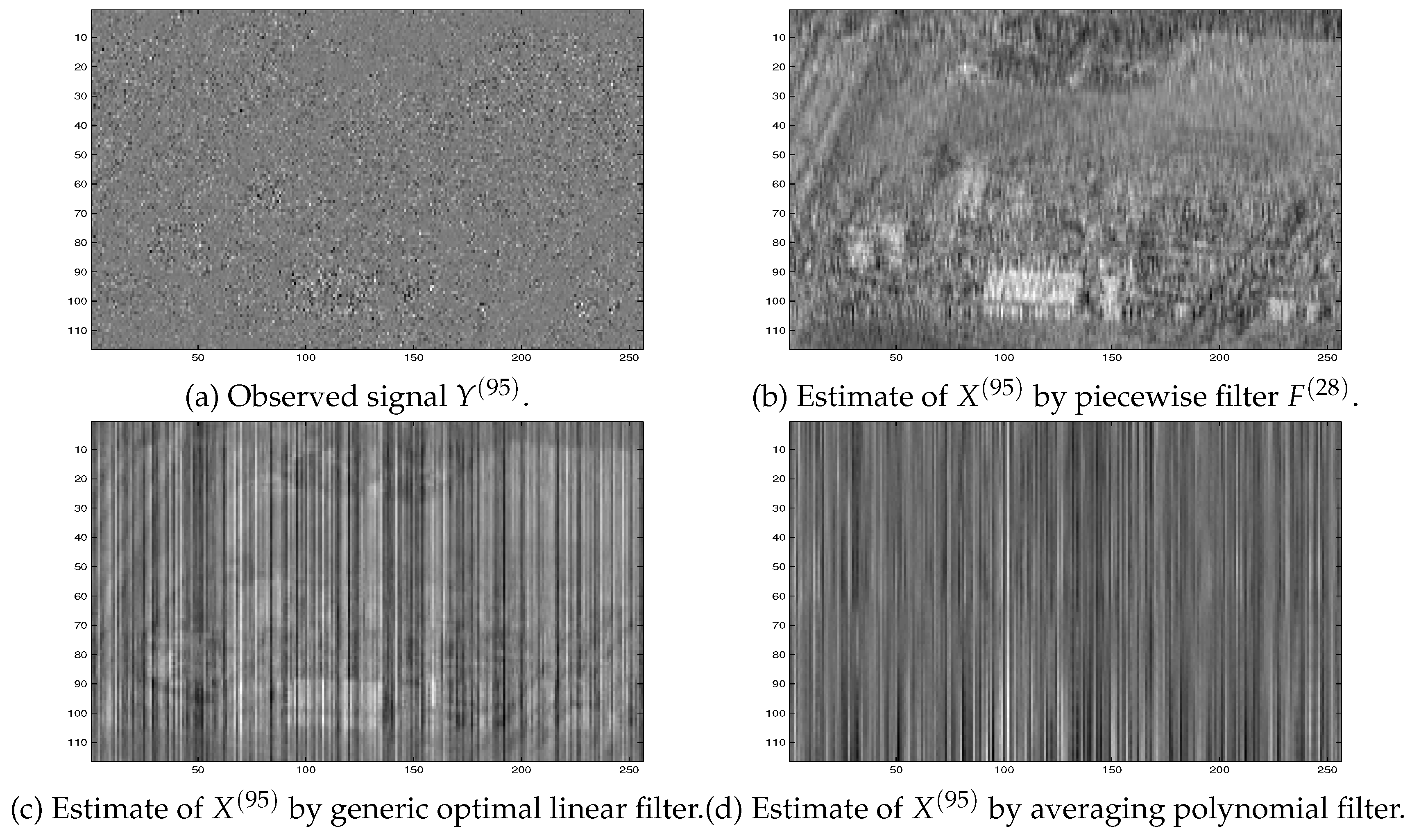
Figure 11.
Illustration of the errors associated with the piecewise interpolation filters and the generic optimal linear (GOL) filters [5] applied to signals described in Examples 1–4.
Figure 11.
Illustration of the errors associated with the piecewise interpolation filters and the generic optimal linear (GOL) filters [5] applied to signals described in Examples 1–4.
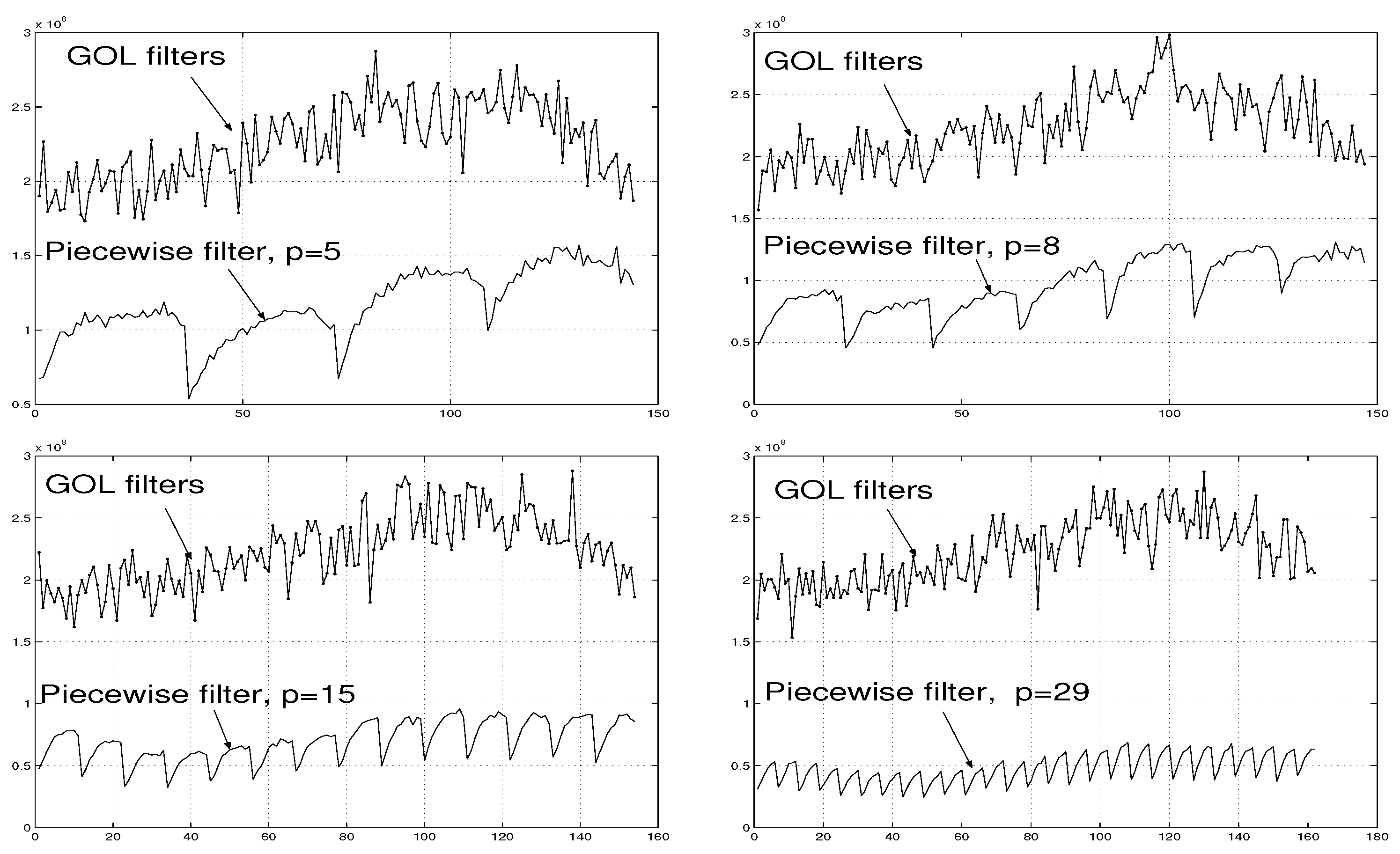
Figure 12.
Examples of selected signals to be estimated from observed data considered in Example 5-9.
Figure 12.
Examples of selected signals to be estimated from observed data considered in Example 5-9.
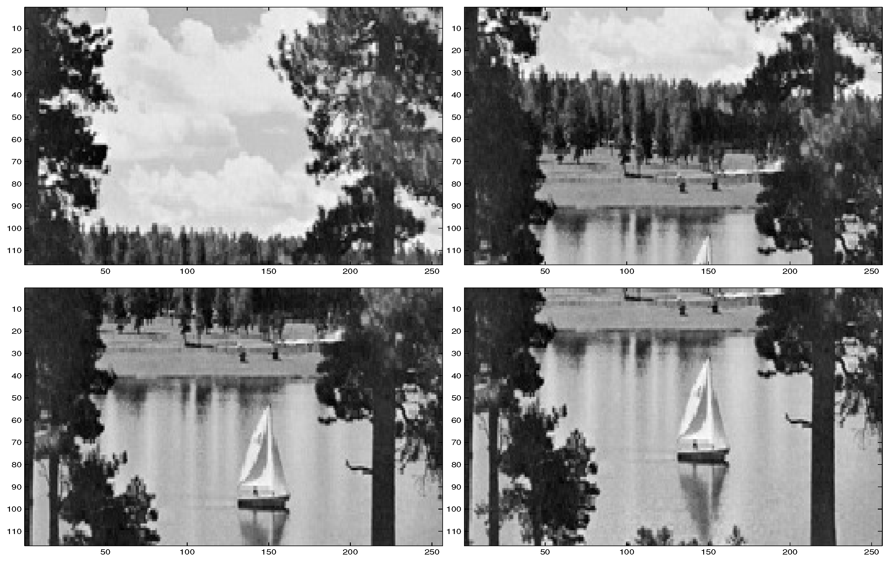
Figure 13.
Examples of the observed signal and the estimates obtained by different filters.
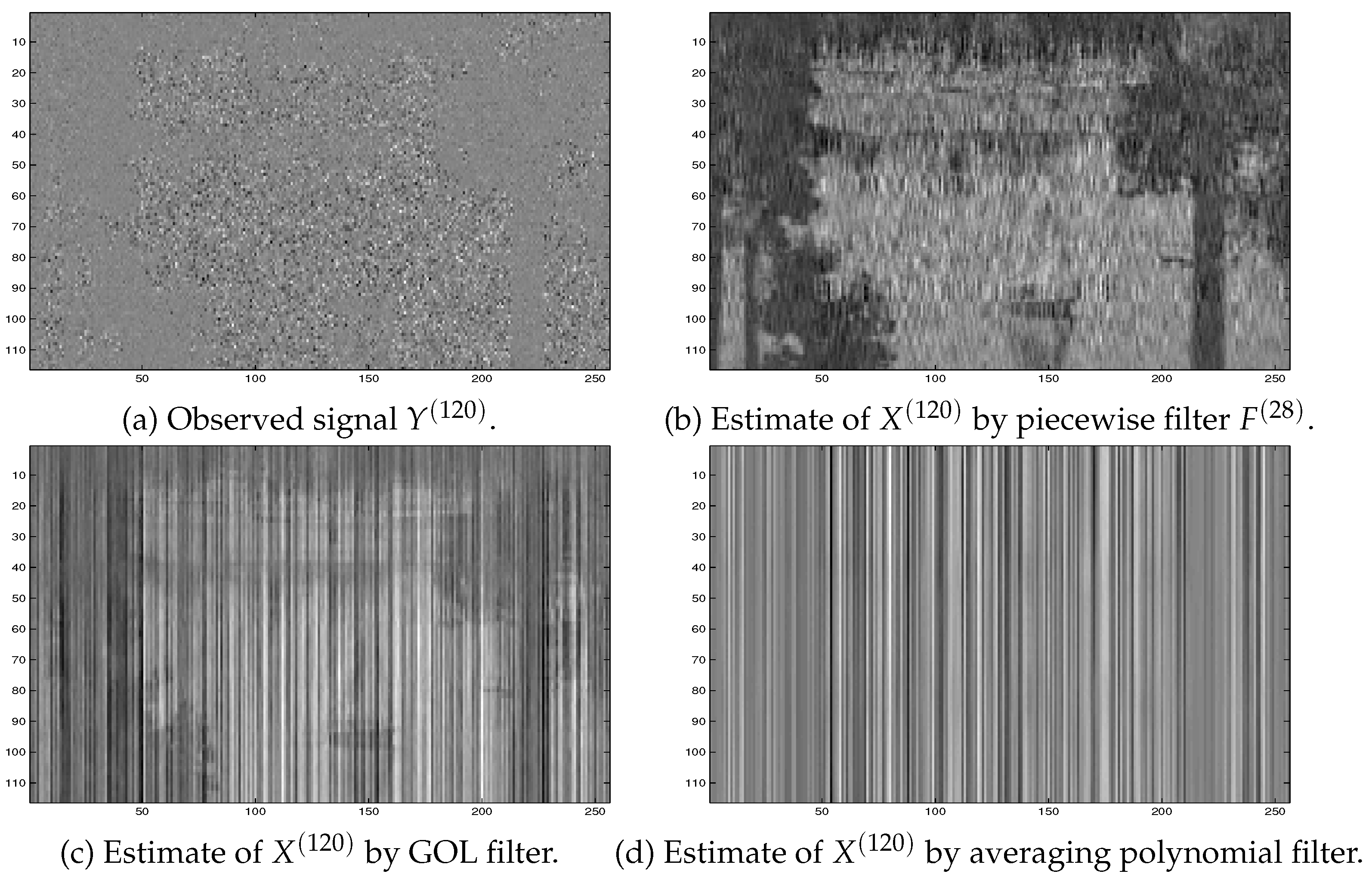
Figure 14.
Illustration of errors associated with the piecewise interpolation filter of order p and the generic optimal linear (GOL) filters [5] applied to signals described in Examples 5–8.
Figure 14.
Illustration of errors associated with the piecewise interpolation filter of order p and the generic optimal linear (GOL) filters [5] applied to signals described in Examples 5–8.
5.6. Summary of Simulations
The above simulations confirm the theoretical results obtained in Theorems 1–3. In particular, Figs. Figure 11 and Figure 14 demonstrate that the error associated with the piecewise interpolation filter decreases when the number of sub-filters , p, increases.
A comparison between the proposed filter and the known related filters [5,10,12,22,23] has been done. The filter estimates the reference signals with the accuracies that are much better than those of the generic optimal linear (GOL) filters [5] and the averaging polynomial filter [10,12]. Further, the filters proposed in [22,23] fail in processing the signals under consideration. This is because the observed signals in (40), (49), (50) and (51) are grossly corrupted and, therefore, the inverse matrices used in the filter structures in [23] do not exist. The technique in [22] requires the use of the reference signal in the proposed filter which is supposed to be unknown in the simulations above.
The filters have been applied to the different signal sets (presented in Section 5.2 and Section 5.3), using different forms of noise (given in (40), (49), (50) and (51)).
computational work associated with the proposed filter is substantially less than that associated with the known filters discussed in Section 1 (in particular, with the filters in [11]–23]). This is because, for the processing of a data set containing N signals, filter requires computation of p covariance matrices with while the known filters require computation of N matrices (in the above Examples, , respectively, and ).
6. Conclusions
The technique of the constructive approximation of a nonlinear operator has been provided. Here, and where and is the set of outcomes of a probability space. The device behind the proposed method is based on a special extension of the piecewise linear interpolation technique to the case of stochastic sets and . The proposed methodology is motivated by the problems arising in signal processing where the nonlinear operator is interpreted as a nonlinear system (or a nonlinear filter) transforming a set of stochastic signals KY to the set of stochastic signals KX Therefore, the provided technique provides an effective way to transform large data sets.
Distinctive features of the approach are as follows.
(i) The proposed filter is nonlinear and is presented in the form of a sum with terms where each term, , is interpreted as a particular sub-filter. Here, and are ‘small’ pieces of and , respectively.
(ii) The prime idea is to exploit a prior information only onfew reference signals, p, from the set that contains signals (or even an infinite number of signals) and determine j separately, for each pieces and , so that the associated error is minimal. In other words, the filter is flexible to changes in the sets of observed and reference signals and , respectively.
(iii) Due to the specific way of determining j, the filter provides a smaller associated error than that for the processing of the whole set by a filter which is not specifically adjusted to each particular piece . Moreover, the error associated with our filter decreases when the number of its terms, , increases.
(iv) While the proposed filter processes arbitrarily large (and even infinite) signal sets, the filter is nevertheless fixed for all signals in the sets.
(v) The filter is determined in terms of pseudo-inverse matrices so that the filter always exists.
(vi) computational load associated with the filter is less than that associated with other known filters applied to the processing of large signal sets.
Authors’ Contributions
Conceptualization, methodology, writing original draft - A.T. Numerical simulations - A.T. and P.P. Algorithm - P.P. Matlab codes - P.P. English amelioration - P.P. The authors have read and agreed to the published version of the manuscript.
Funding
This research received no external funding.
Data Availability Statement
The raw data supporting the conclusions of this article will be made available by the authors on request.
Conflicts of Interest
The authors declare no conflicts of interest.
Appendix A
where is the Frobenius norm. The latter is true because
and
It is known (see, for example, [5], p. 304) that the solution of problem (A5) is given by (19). The equation (17) follows from (6) and (A1).
Theorem 1 is proven. □
Proof of Theorem 2: For and defined by (17)–(19),
Then (A6) implies
where .
It follows from (A2) and (A3) that for given by (19),
Then (16)–(19), (23) and (A6)–(A8) imply that for all and , (24) is true. □
Proof of Theorem 3: The relation (22) implies that
where
Then
Let us consider an estimate of , for . To this end, let us denote .
For i.e. for ,
where . In particular, the latter implies
For i.e. for ,
where . In particular, then it follows that
On the above basis, let us assume that, for with , i.e. for ,
where is defined by analogy with .
Then, for with , i.e. for ,
where . Thus, the following is true:
Therefore, (A10), (A11) and (A12) imply
where , and then it follows from (A9)–(A11) and (A13) that for all ,
Let us now choose and so that and partition interval by points so that and with . There exists an integrable (bounded) function such that, for , . Then
Thus,
References
- Chen, J.; Benesty, J.; Huang, Y.; Doclo, S. New Insights Into the Noise Reduction Wiener Filter. IEEE Trans. on Audio, Speech, and Language Processing 2006, 14(No. 4), 1218–1234. [Google Scholar] [CrossRef]
- Spurbeck, M.; Schreier, P. Causal Wiener filter banks for periodically correlated time series. Signal Processing 2007, 87(6), 1179–1187. [Google Scholar] [CrossRef]
- Goldstein, J. S.; Reed, I.; Scharf, L. L. A Multistage Representation of the Wiener Filter Based on Orthogonal Projections. IEEE Trans. on Information Theory 1998, 44, 2943–2959. [Google Scholar] [CrossRef]
- Y. Hua, M. Nikpour, and P. Stoica, “Optimal Reduced-Rank estimation and filtering,”IEEE Trans. on Signal Processing,vol. 49, pp. 457-469, 2001.
- A. Torokhti and P. Howlett, Computational Methods for Modelling of Nonlinear Systems, Elsevier, 2007.
- E. D. Sontag, Polynomial Response Maps, Lecture Notes in Control and Information Sciences, 13, 1979.
- Chen, S.; Billings, S. A. Representation of non-linear systems: NARMAX model. Int. J. Control 1989, 49(no. 3), 1013–1032. [Google Scholar] [CrossRef]
- V. J. Mathews and G. L. Sicuranza, Polynomial Signal Processing, J. Wiley & Sons, 2001.
- Torokhti, A.; Howlett, P. Optimal Transform Formed by a Combination of Nonlinear Operators: The Case of Data Dimensionality Reduction. IEEE Trans. on Signal Processing 2006, 54(No. 4), 1431–1444. [Google Scholar]
- Torokhti, A.; Howlett, P. Filtering and Compression for Infinite Sets of Stochastic Signals. Signal Processing, 2009; Volume 89, pp. 291–304. [Google Scholar]
- Vesma, J.; Saramaki, T. Polynomial-Based Interpolation Filters - Part I: Filter Synthesis; Circuits, Systems, and Signal Processing, 2007; Volume 26, Number 2, pp. Pages 115–146. [Google Scholar]
- Torokhti, A.; Manton, J. Generic Weighted Filtering of Stochastic Signals. IEEE Trans. on Signal Processing 2009, 57(issue 12), 4675–4685. [Google Scholar] [CrossRef]
- Torokhti, A.; Miklavcic, S. Data Compression under Constraints of Causality and Variable Finite Memory. Signal Processing 2010, 90(Issue 10), 2822–2834. [Google Scholar] [CrossRef]
- Babuska, I.; Banerjee, U.; Osborn, J. E. Generalized finite element methods: main ideas, results, and perspective. International Journal of Computational Methods 2004, 1(1), 67–103. [Google Scholar] [CrossRef]
- Kang, S.; Chua, L. A global representation of multidimensional piecewise-linear functions with linear partitions. IEEE Trans. on Circuits and Systems 1978, 25(Issue:11), 938–940. [Google Scholar] [CrossRef]
- Chua, L.O.; Deng, A.-C. Canonical piecewise-linear representation. IEEE Trans. on Circuits and Systems 1988, 35(Issue:1), 101–111. [Google Scholar] [CrossRef]
- Lin, J.-N.; Unbehauen, R. Adaptive nonlinear digital filter with canonical piecewise-linear structure. IEEE Trans. on Circuits and Systems 1990, 37(Issue:3), 347–353. [Google Scholar] [CrossRef]
- J.-N. Lin and R. Unbehauen, Canonical piecewise-linear approximations,IEEE Trans. on Circuits and Systems I: Fundamental Theory and Applications,39 Issue:8, pp. 697 - 699, 1992.
- Gelfand, S.B.; Ravishankar, C.S. A tree-structured piecewise linear adaptive filter. IEEE Trans. on Inf. Theory 1993, 39(issue 6), 1907–1922. [Google Scholar] [CrossRef]
- Heredia, E.A.; Arce, G.R. Piecewise linear system modeling based on a continuous threshold decomposition. IEEE Trans. on Signal Processing 1996, 44(Issue:6), 1440–1453. [Google Scholar] [CrossRef]
- Feng, G. Robust filtering design of piecewise discrete time linear systems. IEEE Trans. on Signal Processing 2005, 53(Issue:2), 599–605. [Google Scholar] [CrossRef]
- Russo, F. Technique for image denoising based on adaptive piecewise linear filters and automatic parameter tuning. IEEE Trans. on Instrumentation and Measurement 2006, 55(Issue:4), 1362–1367. [Google Scholar] [CrossRef]
- Cousseau, J.E.; Figueroa, J.L.; Werner, S.; Laakso, T.I. Efficient Nonlinear Wiener Model Identification Using a Complex-Valued Simplicial Canonical Piecewise Linear Filter. IEEE Trans. on Signal Processing 2007, 55(Issue:5), 1780–1792. [Google Scholar] [CrossRef]
- P. Julian, A. Desages, B. D’Amico, Orthonormal high-level canonical PWL functions with applications to model reduction,IEEE Trans. on Circuits and Systems I: Fundamental Theory and Applications,47 Issue:5, pp. 702 - 712, 2000.
- T. Wigren, Recursive Prediction Error Identification Using the Nonlinear Wiener Model,Automatica,29, 4, pp. 1011–1025, 1993.
- G. H. Golub and C. F. van Loan, Matrix Computations, Johns Hopkins University Press, Baltimore, 1996.
- T. Anderson,An Introduction to Multivariate Statistical Analysis,New York, Wiley, 1984.
- L. I. Perlovsky and T. L. Marzetta, Estimating a Covariance Matrix from Incomplete Realizations of a Random Vector,IEEE Trans. on Signal Processing, 40, pp. 2097-2100, 1992.
- O. Ledoit and M. Wolf, A well-conditioned estimator for large-dimensional covariance matrices,J. Multivariate Analysis88, pp. 365–411, 2004.
| 1 | We say a stochastic vector is finite if its realization has a finite number of scalar components. |
| 2 | |
| 3 | This means that any desired accuracy is achieved theoretically, as is shown in Section 4.4 below. In practice, of course, the accuracy is increased to a prescribed reasonable level. |
| 4 | As usually, is the set of outcomes, a -field of measurable subsets in and an associated probability measure on . In particular,
|
| 5 | Hereinafter, we will use a non-curly symbol to denote an operator and associated matrix (e.g., the operator and the associated matrix are denoted by ). |
| 6 | It is worthwhile to note that it is not assumed that the covariance matrices are known for each signal pair from , with . |
| 7 | As it has been mentioned in Section 3.4, can be determined by the known methods. |
| 8 | The database is available in http://sipi.usc.edu/services/database.html. |
| 9 | The database is available in http://sipi.usc.edu/services/database.html. |
| 10 | The database is available in http://sipi.usc.edu/services/database.html. |
| 11 | The database is available in http://sipi.usc.edu/services/database.html. |
Disclaimer/Publisher’s Note: The statements, opinions and data contained in all publications are solely those of the individual author(s) and contributor(s) and not of MDPI and/or the editor(s). MDPI and/or the editor(s) disclaim responsibility for any injury to people or property resulting from any ideas, methods, instructions or products referred to in the content. |
© 2025 by the authors. Licensee MDPI, Basel, Switzerland. This article is an open access article distributed under the terms and conditions of the Creative Commons Attribution (CC BY) license (http://creativecommons.org/licenses/by/4.0/).
Copyright: This open access article is published under a Creative Commons CC BY 4.0 license, which permit the free download, distribution, and reuse, provided that the author and preprint are cited in any reuse.


