
Submitted:
08 December 2025
Posted:
09 December 2025
You are already at the latest version
Abstract
Fuel consumption in heavy-duty off-road machinery depends on a wide range of in-teracting factors related to the operating environment, the technical characteristics and condition of the machine, and the behaviour, experience and state of the operator. Existing studies typically address only fragments of this relationship, focusing on vehicle parame-ters, selected environmental factors or individual aspects of driving style. The method proposed in this work provides a general and transferable framework for assessing fuel consumption in any type of machine or vehicle. The Integrated Fuel Consumption As-sessment Model (IFCAM) combines environmental, vehicle and human domains into a coherent structured formula that can be used across different operational contexts. The model was developed using continuous short-term measurements and long-term opera-tional data collected during real industrial work. Its universal structure makes it applica-ble not only to mining equipment, but also to construction machinery and transport vehi-cles, as well as conventional passenger cars, where it offers a systematic procedure for es-timating fuel demand under variable operating conditions. The results demonstrate that integrating multi-domain data improves predictive accuracy and opens new possibilities for analysing operator influence and overall energy efficiency.
Keywords:
fuel consumption
; heavy-duty machines
; construction machinery
; transport vehicles
; operating environment
; vehicle characteristics
; operator behaviour
; integrated assessment model
; machine performance
; IFCAM
1. Introduction
Climate change has been identified for many years as a central global challenge, a conclusion consistently reinforced in successive IPCC assessments, including the 2014 report and the more recent AR6 publication [1,2,3,4]. Both documents emphasise that stabilising greenhouse gas emissions, particularly CO₂, is essential for limiting future environmental and socio-economic impacts. Similar priorities were reflected earlier in the Kyoto Protocol and the Paris Agreement, where emission reductions became a core element of international climate policy [2,3].
Within this context, the transport sector plays a decisive role. Although it is responsible for approximately 22% of global anthropogenic CO₂ emissions, the share attributed to heavy-duty vehicles (HDVs) and specialised machinery is significantly higher than their proportion in the global fleet would suggest [4]. These vehicles operate under demanding conditions, often with long duty cycles, high loads, and limited opportunities for energy recovery, which translates directly into disproportionately high fuel consumption [4,5]. Their role is particularly evident in mining and construction environments, where Non-Road Mobile Machinery (NRMM) powered by internal combustion engines operate round the clock and account for a substantial share of total energy use.
Over the past two decades, both freight activity and the number of HDVs in operation have grown steadily worldwide [6,7]. Long-term projections further indicate that global heavy-duty fleets may nearly double by 2040, resulting in marked increases in fuel demand and related emissions [8,9]. At the same time, regulatory frameworks in the European Union- such as the CO₂ reduction targets for HDVs introduced in 2019- aim to limit these trends while encouraging the development of more efficient powertrains and alternative fuels [10,11]. Industrial analyses suggest, however, that combustion engines will continue to dominate heavy-duty applications in the near future, making improvements in operational fuel efficiency a priority for manufacturers and fleet operators [12].
The scientific literature confirms that fuel consumption in heavy-duty vehicles is shaped by a wide array of factors, including machine characteristics, environmental conditions and human behaviour. Yet most studies examine these factors separately, which limits their usefulness in complex, real-world operating environments. This fragmentation makes it difficult to build models that are both accurate and transferable across vehicle types, operating settings and user profiles.
For this reason, there is a clear need for an integrated assessment method that jointly incorporates environmental, technical and behavioural determinants of fuel consumption. The present work addresses this need by introducing the Integrated Fuel Consumption Assessment Model (IFCAM), a framework developed using real operational data from heavy-duty machinery and applicable to a broad range of vehicles and operating contexts.
2. Literature Review
Fuel consumption in vehicles and heavy machinery has long been recognised as a key parameter affecting operating costs and environmental impact. In recent years, this topic has gained additional relevance due to global efforts to reduce greenhouse gas emissions and improve energy efficiency. Numerous studies have addressed factors that influence fuel use under real operating conditions, focusing on four main areas: vehicle design and technical parameters, environmental and road conditions, driver behaviour, and the type of fuel. Although each of these domains has been investigated extensively, the literature remains fragmented and lacks an integrated approach suited for heavy machinery.
A large body of research examines fuel consumption as a function of vehicle-related parameters. Various methods have been proposed to estimate fuel use on the basis of technical indicators [13,14,15,16,17,18,19]. Many studies focus on the influence of vehicle mass and payload. In [20], the impact of payload mass and road gradient on fuel consumption was analysed, showing that heavier loads increase engine demand and fuel use, especially on gradients above 5%. Other works [21,22,23,24,25,26]confirmed that payload and road infrastructure significantly affect CO₂ and NOx emissions and distance-based fuel consumption. For example, [21] reported that a heavy truck operating with a 20-ton payload showed a 67% increase in fuel consumption in urban conditions and a 45% increase on extra-urban routes. Additional results in [26] indicated that extra-urban cycles reduce fuel consumption by approximately 20% compared with mixed cycles.
Engine power and drivetrain characteristics also play an important role. The analysis in [23] showed that vehicles equipped with higher-power engines exhibited lower fuel consumption and reduced emissions, partly due to the presence of advanced exhaust after-treatment systems. Studies on engine downsizing [27] demonstrated that reducing engine displacement while maintaining power output can lower fuel consumption and emissions. Other works highlighted the influence of drivetrain efficiency, torque characteristics and gear selection on energy use in heavy-duty applications [15,16,18]. A broader technical perspective was provided in [28], where 21 parameters, including vehicle mass, rolling resistance, drivetrain losses and aerodynamic characteristics, were identified as significant determinants of fuel consumption.
Environmental and climatic conditions form the second major group of factors. In [29]the relationship between ambient temperature, rolling resistance, air density and drivetrain efficiency was analysed. Temperature variations from -15 °C to +30 °C were shown to cause measurable changes in fuel consumption, with a minimum at around 9 °C and an increase of about 7% at temperature extremes. Lower temperatures increase rolling resistance and air density, contributing to higher energy demand. Similar relationships were observed in studies addressing the combined effects of terrain, atmospheric pressure, microclimate and road surface [20,29,30,31,32,33]. Recent findings [34] emphasise the growing importance of high-resolution environmental modelling due to the non-linear behaviour of modern propulsion systems, including hybrid and regenerative systems.
Road geometry also has a substantial impact on fuel use. In [35], a predictive cruise-control algorithm was introduced that uses rolling resistance, aerodynamic drag and gravitational forces to anticipate engine load. This approach resulted in a 3.5% reduction in fuel consumption over a 120 km route and a 42% reduction in gear shifts. A related mathematical model in [36]quantified the influence of speed, elevation and gradient on fuel consumption in mountainous conditions. Simulations and fleet analyses in [37] further indicated that omitting slope dynamics and transient load responses can lead to errors exceeding 15% in fuel consumption estimation.
Human behaviour is another decisive factor. Numerous studies [38,39,40,41,42]have shown that driving style, particularly rapid acceleration, high speed variability and unnecessary braking, significantly affects fuel consumption. These findings form the basis for eco-driving strategies. Research on eco-driving [40,41,42,43,44,45,46,47,48] reports potential fuel savings of up to 15% [49]. However, long-term improvements are limited because drivers tend to return to previous habits [50], and awareness regarding the impact of driving style remains low [51]. Other studies pointed to the limited use of incentive systems for fuel-efficient driving [52,53]. Sustainable reductions in fuel consumption therefore require continuous monitoring of driver behaviour and operating parameters [54].
The literature also addresses broader human factors. The influence of emotional state [38,55,56], aggression [57,58], fatigue, health status [59,60,61,62], skills [50], age [63,64] and use of intoxicants [62,65,66] on driving behaviour and fuel consumption has been documented. Behavioural variability between operators is now recognised as one of the largest sources of uncertainty in predictive models, which is consistent with recent findings presented in [67].
Fuel type and composition constitute another important research area. Numerous works have examined the performance and environmental implications of biofuels and fuel blends, including FAME and FAEE esters [68], palm-oil-derived fuels [69], diesel–natural gas dual-fuel systems [70], bioethanol blends [71] and fuels containing nanomaterial additives [72]. Many studies showed that although specific fuel consumption may be higher due to lower calorific value, renewable fuel components improve overall environmental performance. Research on glycerol-based fuels [73,74] and locally developed blends [75,76,77] identified further options for low-cost, low-carbon solutions. In [78], adding 30% n-butanol reduced CO₂ emissions and lowered fossil-carbon content due to the biogenic share of the fuel.
Modelling and prediction of fuel consumption are also widely addressed. Classical regression models and combustion-process analyses [79,80,81] have been complemented by machine-learning approaches using neural networks and multi-parameter telematics data. Large data sets derived from CAN-bus and OBD systems enable the development of advanced predictive models [34,67]. These studies show that traditional assessment methods require updating, as they do not fully reflect current vehicle technologies, duty cycles or energy management strategies. This view is consistent with findings in [82], which highlight limitations of existing frameworks such as HDM-4 and the need for their recalibration.
In summary, fuel consumption has been studied extensively for many decades, and remains central to international strategies aimed at reducing emissions. Despite the wide range of existing research, knowledge is dispersed across separate domains, and there is no comprehensive method that integrates vehicle parameters, environmental factors and human behaviour. This gap is particularly evident for heavy machinery, which will continue to rely on combustion engines for many years. These observations justify the development of a systematic and transferable fuel consumption assessment method.
3. Model and Methodology
The fuel consumption assessment method proposed in this study is based on the practical observation that fuel use in heavy-duty machinery results from the interaction of three areas operating simultaneously. These include the operating environment, the technical characteristics of the vehicle and the human factor associated with the operator. In practice, these three domains form a single interacting system, and fuel consumption is the measurable outcome of their combined effect. This concept, frequently highlighted in operational studies of transport and mining machinery, is reflected in the Environment - Vehicle - Human diagram, where fuel consumption remains at the centre of the interaction.
The development of the method followed a sequence that mirrors the logic of real data processing. At the beginning, it was necessary to define the boundaries of the system by specifying criteria such as dataset size, data homogeneity, availability and the possibility of completing missing records. Only after meeting these requirements was it possible to proceed with the main analytical stages: data collection, verification of raw signals, construction of individual models and validation of the selected variables. These stages correspond directly to the workflow shown in the methodological diagram and illustrate how raw operational data are transformed into a structured analytical model.
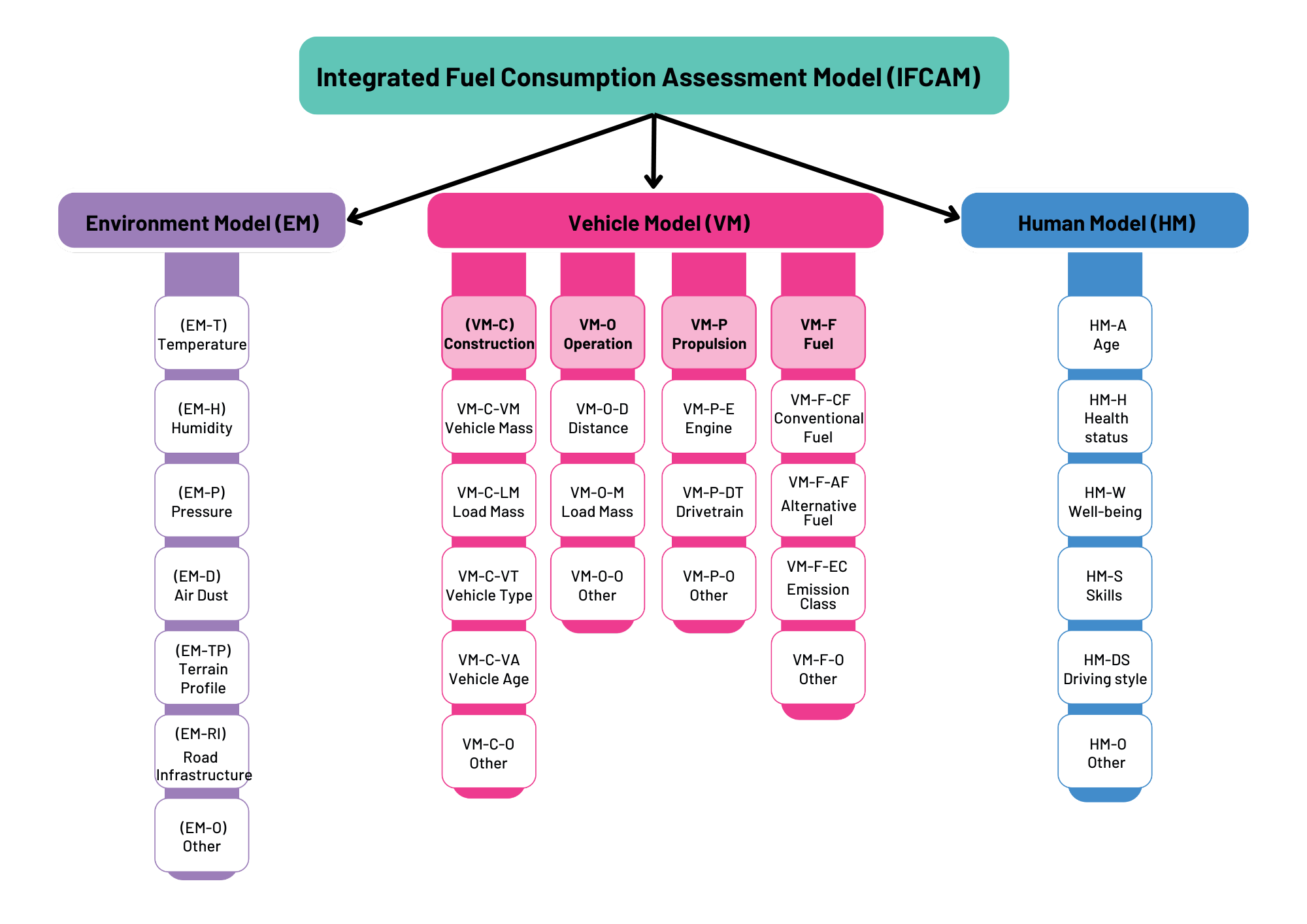
The central component of the method is the Integrated Fuel Consumption Assessment Model (IFCAM). This structure groups all relevant variables into three coherent areas: the Environment Model (EM), the Vehicle Model (VM) and the Human Model (HM). The EM includes parameters typical for underground and open-pit conditions, such as temperature, humidity, pressure, dust level, terrain profile or road infrastructure. The VM comprises construction-related factors, operating conditions, engine and drivetrain characteristics and the type of fuel used. The HM includes operator-related features such as age, health status, well-being, skills and driving style, which directly influence the energy demand of the machine.
A key feature of the IFCAM structure is the clear placement of each parameter within its functional category. This makes the model scalable and adaptable to other machine types, construction equipment and road transport fleets. Its modular architecture also allows for further extensions, for example by including new vehicle propulsion technologies or additional behavioural indicators.
In the final stage, the validated EM, VM and HM variables are integrated into the fuel consumption model, which becomes the basis for subsequent analytical and optimisation tasks. Although this paper does not discuss the operator efficiency index or neural network prediction modules, the method preserves the ability to incorporate these elements in separate studies.
Overall, the diagrams used in this section illustrate how the assessment method progresses from defining the operational system, through modelling the three core domains, to the final integration step that forms the IFCAM model. Taken together, these components provide a transparent and consistent methodology for evaluating fuel consumption under real and continuously changing operating conditions.
3.1. Structure of the Integrated Fuel Consumption Assessment Model
The Integrated Fuel Consumption Assessment Model (IFCAM) is built on three fundamental components: the Environment Model, the Vehicle Model and the Human Model, as shown in Figure 1. Each component groups variables that describe a separate area of influence on fuel consumption. The model can be applied to different types of machinery, including underground and surface mining equipment, construction machines, transport vehicles, agricultural machinery and specialised industrial vehicles. The mining case presented in this study serves only as an example of implementation.
3.1.1. Environment Model (EM)
The Environment Model groups external physical and infrastructural conditions in which the machine operates. These factors do not depend on the vehicle or the operator and describe the characteristics of the location in which the machine performs its tasks.
The EM includes the following variables:
- EM-T– temperature: ambient temperature in the working area,
- EM-H– humidity: relative air humidity,
- EM-P– atmospheric pressure: pressure at the operating site (e.g. depth underground or altitude above sea level),
- EM-D– dust level: concentration of airborne particulate matter,
- EM-TP– terrain profile: geometry of the ground or roadway, including inclines and local variations,
- EM-RI– road or ground infrastructure: surface type and condition,
- EM-O– other environment-specific parameters: factors characteristic for a specific location.
The Environmental Model is expressed as:
3.1.2. Vehicle Model (VM)
The Vehicle Model describes the characteristics of the machine itself. It consists of four sub-models: Construction, Operation, Propulsion and Fuel. This structure allows the model to be used for different machine types and applications.
- 1.
-
Vehicle Construction Sub-Model ( VM-C)
- VM-C-VM– vehicle mass (empty): base mass of the machine,
- VM-C-LM– load mass: mass of the transported material,
- VM-C-VT– vehicle type: classification based on function and configuration,
- VM-C-VA– vehicle age: age or hours of operation,
- VM-C-O– other construction parameters.
- 1.
-
Vehicle Operation Sub-Model ( VM-O)
- VM-O-D – distance or operating cycle type,
- VM-O-M – load-related operational mass,
- VM-O-O – other operating variables.
- 2.
-
Vehicle Propulsion Sub-Model ( VM-P)
- VM-P-E – engine: main propulsion unit,
- VM-P-DT – drivetrain: type of transmission system,
- VM-P-O – other propulsion-related factors.
- 3.
-
Vehicle Fuel Sub-Model ( VM-F)
- VM-F-CF – conventional fuel: standard diesel or gasoline fuels,
- VM-F-AF – alternative fuels: biodiesel, dual-fuel or hybrid mixtures,
- VM-F-EC – emission class: emission category of the vehicle,
- VM-F-O – other fuel-related parameters.
VM − F = f(VM − F − CF, VM − F − AF, VM − F − EC, VM − F − O)
3.1.3. Human Model (HM)
The Human Model groups operator-related factors that can influence fuel consumption. These parameters describe the physical and behavioural characteristics of the driver.
- HM-A – age.
- HM-H – health condition.
- HM-W – well-being.
- HM-S – skills and training level.
- HM-DS – driving style.
- HM-O – other operator-related variables.
The detailed structure of the Integrated Fuel Consumption Assessment Model is presented in Figure 2.
3.1.4. Final Integrated Fuel Consumption Formula
The complete model is obtained by integrating the three domains:
In expanded form:
The functional form does not require all variables to be present in every use-case. Empty variables are treated as non-active parameters, allowing the model to be applied in sectors where only a subset of EM, VM or HM inputs is available.
The method is based on the sequence of steps used in the processing of operational data: system definition, data acquisition, verification, model construction and analytical integration. The workflow illustrates how raw machine data are transformed into an analytical structure.
After defining the complete functional form of the fuel consumption model, the next step is to link the mathematical structure with the practical workflow used to develop and apply the Integrated Fuel Consumption Assessment Model. The sequence presented in Figure 3 shows the full procedure, starting from system definition and ending with decision-making and long-term monitoring. Each stage corresponds directly to the steps required to transform raw operational data into a validated and transferable fuel consumption model.
The first block of the schematic refers to the system establishment stage, in which the operational context and analytical constraints are defined. This includes specifying the dataset size, its homogeneity, completeness and the feasibility of supplementing missing segments. These criteria ensure that all three domains- Environment, Vehicle and Human- are represented with sufficient resolution to construct stable statistical models.
The next stages, data collection and data verification, reflect the practical process of acquiring and preparing raw signals. Data verification includes identification and removal of corrupted records, detection of missing values, spikes and outliers, as well as the assessment of internal consistency between related parameters. At this point, each variable is assigned to its proper category within the EM, VM or HM domain, which ensures correct interpretation during model development.
Following verification, the individual domain models are developed. This stage includes statistical evaluation of each parameter, its preliminary correlation with specific fuel consumption and the construction of regression-based functional dependencies, consistent with the approach used in the doctoral research. Model validation follows, comprising tests of statistical significance of coefficients, analysis of residuals, assessment of model stability and the examination of multicollinearity. Variables that demonstrate instability or lack of statistical relevance are eliminated. The validated EM, VM and HM models are then used to assess relationships between the domains and to identify dominant factors or interactions that influence fuel consumption.
The final part of the schematic shows the transition from model development to application. The validated variables are integrated into the full fuel consumption model, which can be used for several analytical purposes:
- short-term prediction, for example by applying neural networks to forecast fuel consumption over a future time interval Δt;
- operator performance assessment based on the efficiency index e, used for comparative analysis between operators or shifts;
- local decision-making within a selected Environment, Vehicle or Human domain, allowing adjustments to operational practices or machine parameters;
- global decision-making, supporting fleet-level or organisational strategies aimed at reducing fuel consumption;
- long-term data management, enabling continuous monitoring of changes in the system and updating the model when new operational conditions occur.
The schematic therefore summarises not only the construction of IFCAM but also the entire procedure required for its practical implementation. Because each element of the workflow is independent and modular, the method can be applied across various sectors beyond mining, including construction machinery, agricultural equipment, municipal service vehicles and heavy road transport. The only requirement is that the available operational variables are assigned to the relevant EM, VM or HM categories. Once this condition is met, the same workflow can be followed to construct a complete and transferable fuel consumption model.
4. Study System and Data (Corrected and Validated)
The Integrated Fuel Consumption Assessment Model (IFCAM) was developed using long-term operational data from a large underground mining complex in Europe. The system comprises three underground mines with a combined annual ore production of approximately 30 million tonnes. Mining is carried out at depths of about 1000–1200 m, where the geothermal gradient reaches roughly 1°C per 32 m of depth, resulting in high ambient temperatures in the working areas.
4.1. Environmental Conditions
The analysed mine operates in demanding thermal and atmospheric conditions typical for deep underground extraction. Daily measurements collected across more than ten production districts showed:
- dry-bulb temperature (EM–T): 33.7–37.0°C,
- climate substitute temperature: 28.9–31.0°C,
- relative humidity (EM–H): ≈90%,
- airflow velocity (EM–O): 0–2 m/s,
- dust concentration: high and stable,
- roadway inclination: ≤5°,
- roadway dimensions:
– width ≥ 4.6 m,
– height typically 2–4 m, depending on ore thickness.
These values are consistent with the geothermal conditions of underground workings at depths above 800 m, where rock temperatures reach +35 to +46°C, requiring the use of central cooling installations with cooling capacities above 15 MW.
The environmental characteristics listed above were used directly in the Environment Model (EM), as they represent the physical boundary conditions under which LHD machines perform repetitive loading–hauling–dumping cycles.
4.2. Vehicle Population and Machine Selection
The mining company operates a fleet of approximately 1200 heavy-duty vehicles, including trucks, loaders, drilling rigs and auxiliary machinery. Within the analysed mine, 507 machines operate underground.
For IFCAM validation, a homogeneous population of 45 loading machines (LHDs) was selected from a total of 123 loaders in the fleet. This group was chosen because:
- all machines shared the same engine type and drivetrain configuration,
- they performed the same type of work (short-distance loading and hauling),
- they represented the highest annual fuel consumption within their category.
The annual fuel use of these 45 loaders exceeded 4.14 million litres, making them the most fuel-intensive group on site.
Typical technical properties of the selected LHD class include:
- bucket capacity: ≈4.6 m³,
- machine operating weight: ≈28.7 t.
These characteristics correspond to the parameters included in the Vehicle Model (VM), particularly in construction-, operation- and propulsion-related components. To illustrate the operating conditions and the type of machinery included in the study, two representative photographs of underground loading equipment are shown below. The images on Figure 4 document the typical working environment, roadway geometry, dust level and spatial limitations characteristic of the analysed system. They also reflect the conventional configuration of the LHD loader class selected for IFCAM validation.
4.3. Human-Related Factors
The dataset included 41 operators assigned to the selected LHD group. Each operator worked underground for approximately 6 hours per shift in a four-shift system.
Although detailed demographic data (age, health records) were not available, all operators met the required medical and training criteria for work in deep underground conditions.
The only operator-related factor that could be reliably assessed was the driving style, represented in the data by:
- engine speed n,
- engine torque M,
- effective work time t,
- transported material mass per cycle,
- instantaneous fuel use.
These behavioural differences were included in the Human Model (HM). No unsupported numerical ranges describing fuel variability were added.
4.4. Monitoring System and Data Structure
All selected machines were equipped with an on-board diagnostic and monitoring system recording data with a frequency of 1 Hz. The system captured over 30 separate parameters, including:
- engine state variables,
- drivetrain load and temperatures,
- hydraulic system pressures and temperatures,
- payload measurements,
- selected environmental indicators.
This temporal structure allowed the IFCAM method to be applied consistently across machines performing repetitive tasks under similar boundary conditions.
4.5. Data Pre-Processing
Data pre-processing followed a structured multi-stage verification procedure:
- 3–7% of records were removed due to missing data, corrupted values or unrealistic spikes,
- only short gaps of ≤2–3 seconds were interpolated,
- after verification, 93–97% of all signals remained valid,
- all four phases of the operational cycle (loading, loaded haul, dumping, return) were automatically identified and aligned.
This ensured that the dataset fulfilled the requirements of IFCAM regarding completeness, homogeneity and repeatability. This ensured that the dataset fulfilled the requirements of IFCAM regarding completeness, homogeneity and repeatability. The key characteristics of the validated dataset are summarised in Table 1.
5. Results and Analysis
The Integrated Fuel Consumption Assessment Model (IFCAM) was applied to the operational dataset obtained from the underground mining system discussed in Section 4. The purpose of this part of the study is to examine how the three components of the model– environment, vehicle and operator– shape fuel consumption during real repetitive loading–haul–dump cycles.
In this article IFCAM is demonstrated on one industrial case: an underground copper mine in Europe. The site was selected because it provides continuous work cycles, stable boundary conditions and long-term monitoring data. These features make it suitable for validating the method, even though IFCAM itself is not limited to mining applications and can be transferred to other heavy-duty vehicles.
To ensure a consistent analytical sample, the study focused on one machine class operated in large numbers at the site. Out of 45 LHD loaders equipped with the same engine and drivetrain configuration, 38 units met the completeness criteria and were included in the analysis. This allowed the dataset to remain homogeneous while still providing sufficient statistical diversity for model validation. The same selection logic can be applied to other groups of machines when IFCAM is used in different sectors.
The sections that follow present the results obtained for the environmental, vehicle and operator domains, as well as the combined relationships between these factors. All results are based solely on the measured 1 Hz data without introducing external assumptions.
5.1. Environmental Conditions and Their Impact on Fuel Use
Validation of the Environmental Model (EM) focused on assessing which environmental parameters showed sufficient variability and statistical relevance to be included in the final IFCAM structure. Long-term operational measurements demonstrated that most environmental variables characteristic for the analysed system remained effectively constant throughout machine operation. Relative humidity (≈90%), dust concentration (high and stable), roadway inclination (≤5°) and airflow velocity (0-2 m/s) did not exhibit meaningful variation and were therefore excluded from regression analysis. Their role in the model is structural- they define the boundary conditions of the operating environment, but they do not contribute to explaining fuel consumption differences between machines.
Among all EM variables, dry-bulb temperature (t_a) was the only parameter that varied sufficiently (33.7-37.0 °C) to assess its direct influence on hourly fuel consumption. This allowed for a focused validation consistent with the model-selection procedure used in the full IFCAM framework. The applied analyses included exploratory statistics, correlation testing and second-order curve fitting to capture potential non-linear effects.
The results confirmed that temperature had a statistically relevant but moderate effect on fuel consumption. The relationship is shown in Figure 5, where the distribution of data points and the fitted polynomial curve indicate a non-linear trend: fuel consumption decreases slightly around intermediate temperatures and increases noticeably above approximately 36.5 °C. This behaviour is consistent with known thermal effects on air density, engine efficiency and mechanical losses in heavy-duty diesel engines. The calculated Pearson correlation coefficient (r = 0.20) also confirms a measurable, though not dominant, influence.
Although temperature explains a smaller share of variability compared with the Vehicle Model (VM) and Human Model (HM), including this variable improved overall model stability and reduced residual error. Importantly, the environmental conditions presented in this study represent only an application example, demonstrating how IFCAM identifies and validates relevant environmental predictors. The same procedure can be applied in construction, transport or agricultural machinery, where environmental parameters may vary more widely and thus contribute more substantially to fuel consumption.
5.2. Vehicle Model (VM) Validation
The Vehicle Model (VM) was initially structured into four conceptual groups: (i) vehicle construction, (ii) operating profile, (iii) propulsion system, and (iv) fuel type. In the present case study, all analysed machines belonged to the same class of underground wheel loaders, equipped with the same diesel engine, identical drivetrain layout and supplied exclusively with standard diesel fuel. As a result, several construction- and fuel-related variables remained constant across the fleet and could not be used as explanatory predictors in the regression layer of IFCAM. Their role is structural: they define the machine class and boundary conditions of the analysed system.
A full dataset was available for 38 machines of the same model, each of which operated for a complete year without long shutdowns. For every machine, monthly and annual fuel consumption and operating hours were recorded, allowing the calculation of average hourly fuel consumption HFC [dm³/h] at both monthly and annual levels. In 2021 the highest monthly average HFC was observed in December (25.42 dm³/h), while the lowest was recorded in May (23.21 dm³/h). The overall mean for the fleet was 24.37 dm³/h. At the machine level, the most fuel-intensive unit reached an annual average of 28.58 dm³/h, whereas the lowest value was 21.25 dm³/h.
5.2.1. Machine Age and Fuel Consumption
Machine age (in decimal years since commissioning) was first evaluated as a potential VM predictor. Normality of its distribution was checked using several tests: Kolmogorov–Smirnov, Lilliefors, Shapiro–Wilk and D’Agostino–Pearson. Although the Kolmogorov–Smirnov test suggested approximate normality (p = 0.288), the more sensitive tests for small samples (n = 38) indicated that the age distribution significantly deviated from normality (Lilliefors p = 0.021, Shapiro–Wilk p = 0.036, D’Agostino–Pearson p = 0.023). This justified the use of non-parametric correlation methods.
The monotonic dependence between machine age and average annual HFC was therefore analysed using Spearman’s rank correlation. The resulting coefficient was r = −0.174 with p = 0.295 (95% CI: −0.48 to 0.16), which confirms the absence of a statistically significant relationship between age and hourly fuel consumption. The corresponding scatter plot (Figure 6) shows considerable dispersion of points without a clear trend, supporting this conclusion.
In a second step, the correlation between machine age and total annual fuel consumption (sum of fuel dispensed in 2021) was evaluated. In this case a strong, statistically significant negative correlation was observed, with Spearman r = −0.686 (95% CI: −0.83 to −0.46, p = 0.000002). Older machines consumed significantly less fuel per year, which reflects their reduced utilisation rather than improved energy efficiency. This result is important for IFCAM: age acts as a utilisation indicator at fleet level, but it does not explain differences in specific hourly consumption between machines.
5.2.2. Fleet-Level Consistency of Hourly Fuel Consumption
A key methodological question for IFCAM was whether a single representative machine could be used for detailed telemetric analyses, instead of processing complete high-frequency data from all 38 units. To address this, statistical tests were carried out to verify the consistency of HFC across machines and months.
First, a non-parametric repeated-measures ANOVA (Friedman test) was applied to monthly HFC values for all machines in 2021. The test compared fuel consumption across the twelve months for the entire fleet. The Friedman statistic was T₁ = 19.25 with p = 0.0568, slightly above the conventional 0.05 threshold. This indicates that no statistically significant differences in hourly fuel consumption between months were detected, even though some months exhibited slightly higher median values (e.g., March and October), as illustrated in Figure 7.
Figure 8 presents the distribution of hourly fuel consumption (HFC) for all 38 machines across fourteen consecutive months (November 2020–December 2021). The results show that HFC remains within a narrow and stable range of approximately 23–26 dm³/h throughout the entire observation period. Median values for all months are closely aligned, and interquartile ranges are relatively uniform, indicating comparable loading conditions and similar operational profiles over time.
A small number of outliers correspond to isolated periods of higher engine load but do not alter the overall distribution pattern. Importantly, no visible month-to-month shift in central tendency or dispersion is observed. This visual inspection is consistent with the Friedman test, which did not identify statistically significant differences in HFC between months.
The stability of monthly HFC distributions confirms that the fleet operates under consistent duty cycles and supports the methodological assumption that a single unit can be treated as representative for high-resolution telemetric analyses within IFCAM.
Next, the Kendall’s coefficient of concordance W was used to assess the agreement of HFC values between machines across months. In this formulation, each machine acted as a “judge” assigning ranks to months (or conversely, each month acted as a judge ranking machines). The resulting coefficient was W = 0.385, with an associated chi-square statistic of 170.82 and p < 0.000001. The corresponding average pairwise Spearman correlation between machines was 0.329. These values indicate a moderate but statistically highly significant level of agreement in hourly fuel consumption across the fleet.
Together, the Friedman and Kendall tests support the hypothesis that the machines exhibit statistically consistent hourly fuel consumption behaviour over time. On this basis, the following working hypothesis was accepted:
H1.
A single machine of the analysed type can be treated as representative of the entire fleet with respect to hourly fuel consumption.
This conclusion is essential for the design of IFCAM. It justifies the reduction of data volume by focusing detailed, high-frequency analyses (e.g., engine speed, torque, instantaneous fuel rate, bucket load) on one carefully monitored reference machine, while fleet-level effects remain captured by aggregated VM parameters (age, utilisation and HFC distributions).
5.2.3. Implications for the Vehicle Model in IFCAM
In summary, VM validation for this case study showed that:
- Construction-related and fuel-related parameters remained constant and therefore define the machine class rather than explain variability in fuel consumption.
- Machine age does not significantly influence average hourly fuel consumption, but it is strongly and inversely correlated with annual fuel use due to reduced utilisation of older machines.
- Hourly fuel consumption patterns are statistically consistent across the 38 machines, which validates the use of a single representative machine for in-depth telemetric analysis within IFCAM.
As a result, the Vehicle Model in this implementation of IFCAM incorporates age and utilisation measures at fleet level, while load- and engine-related variables derived from telemetric data are further analysed within the Human Model (HM), where they are attributed to operator behaviour rather than to the vehicle itself.
4.3. Validation of the Human Model (HM)
The Human Model (HM) component of the fuel-consumption framework was validated using high-resolution telemetric data obtained from one load–haul–dump (LHD) machine operated over 18 days by 41 operators. The objective of this analysis was to isolate and quantify the behavioural contribution to fuel consumption under stable environmental, organisational and vehicle-related conditions. Since individual-level demographic or physiological data (age, training level, fatigue, health status) were not available, operator influence was inferred exclusively from behavioural patterns represented in engine-related variables. This approach is consistent with contemporary research demonstrating that behavioural signatures—rather than self-reported characteristics—are often the most reliable proxy for driver-induced variability in energy demand.
4.3.1. Data Characteristics and Behavioural Indicators
The telemetric system recorded engine speed (rpm), engine torque (T), instantaneous fuel rate, specific fuel consumption (SFC, g/kWh) and, where available, bucket load mass (m). Across several hundred thousand observations sampled at 1 Hz:
- mean rpm ≈ 1539,
- mean torque ≈ 483 Nm,
- mean SFC ≈ 208 g/kWh, close to the nominal 205 g/kWh reference,
- operator-level SFC ranged widely between ≈184 g/kWh and ≈236 g/kWh.
This wide dispersion occurred despite all operators using the same machine, in the same environment, and performing the same task- strongly suggesting a behavioural origin rather than mechanical or contextual causes. Missing data in bucket-load measurements indicated inconsistencies in the measurement system; however, where mass data were available, distribution patterns provided additional behavioural context. Normality tests (Kolmogorov–Smirnov, Lilliefors) confirmed non-normal distributions for all variables (p < 0.01), necessitating non-parametric statistical methods.
4.3.2. Operating-Field Analysis
To evaluate how operators utilise the available powertrain, operating points were mapped into the (rpm–T) plane and binned into 45 subregions representing distinct operating states ranging from idle/low-load to near-maximum power. The distribution of engine operating points across the torque–speed domain is shown in Figure 9, where the heat-map visualization highlights the most frequently utilized operating ranges.
This analysis revealed strong behavioural clustering:
- operators spent only ~3% of time in the most fuel-efficient SFC region (≈180–200 g/kWh),
- ~9% in the extended efficient region,
- ~97% of total operating time was located in regions where SFC exceeded 200 g/kWh.
Two areas dominated:
- Low-load operation (idle and low rpm): large clusters appeared around 800–1000 rpm and torque below 200 Nm. Although these points represent low mechanical load, they are inefficient because fuel is consumed without producing useful work.
- High-load, high-rpm operation: dense clusters also emerged above 1600 rpm and in torque ranges approaching machine limits (≈850–1000 Nm). In these regions SFC increases sharply due to enriched fuel dosing, thermal stress and reduced combustion efficiency. Together, these patterns indicate that operators rarely utilise the machine in the thermodynamic “sweet spot” identified in engine efficiency theory.
The analysis also demonstrates that behaviourally induced inefficiency overwhelms the mechanical capacity for optimal performance — an important finding for energy-intensive sectors.
4.3.3. Efficient vs. Inefficient Operators: Behavioural Signatures
To isolate behavioural effects, operators were ranked by mean SFC, considering only those with ≥2.5 h of recorded work to ensure representativeness, shown on Figure 10.
Efficient operators (SFC ≈ 200–201 g/kWh)
These operators exhibited:
- 59–75% of operating time in low- and mid-speed regions (800–1600 rpm),
- minimal sustained operation at high torque/speed,
- smooth, evenly distributed operating-point fields.
Their rpm–SFC curves showed a predictable pattern: SFC rises gradually with rpm up to ~1500 rpm, then stabilises around ~210 g/kWh — typical of conservative, controlled driving.
Inefficient operators (SFC ≈ 232–236 g/kWh)
In contrast, inefficient operators:
- spent 52–58% of time above 1600 rpm,
- showed pronounced clustering near the machine’s upper speed and torque limits,
- displayed distinct “bands” of high SFC (220–240 g/kWh) across large rpm intervals.
Their behaviour indicates persistent operation in high-load states, consistent with over-aggressive throttle application, insufficient modulation and prolonged peak-power usage. These behavioural archetypes correspond well with human-factor findings in heavy-vehicle operations: operators with smoother pedal modulation and load anticipation consistently achieve lower energy consumption.
Spearman correlation analysis conducted for the full dataset revealed the following relationships:
- engine speed and torque were highly positively correlated (r ≈ 0.78), which reflects the mechanical interaction between throttle application and engine-load generation;
- both variables showed a moderate positive correlation with specific fuel consumption (r ≈ 0.47–0.49), indicating that increases in speed and load lead to higher fuel demand;
- bucket payload exhibited only a weak, although statistically significant, correlation with fuel consumption, suggesting that the presence of load contributes to fuel use, but its influence is secondary relative to operator-induced changes in speed and torque.
To verify whether bucket load introduced meaningful differentiation, the dataset was divided into two subsets:
- m ≤ 0.05 t (nominally no-load operation),
- m > 0.05 t (operation with measurable load).
A Mann–Whitney U test confirmed statistically significant differences in fuel-consumption distributions between these groups (p < 0.05); however, the magnitude of the effect was small. This result supports the interpretation that for this machine type, fuel consumption is predominantly driven by operator behaviour rather than by variations in transported mass.
4.3.5. Implications for the Human Model and Energy Efficiency
The validation outcomes clearly indicate that operator behaviour constitutes the dominant source of variability in fuel consumption when environmental and machine-level conditions remain stable. This leads to several practical insights:
- Differences attributable to individual operators exceed those originating from machine tolerances. Under identical conditions, variations in SFC between operators reached 28–30%.
- Operators rarely utilise the most efficient operating region; time spent in these favourable ranges amounted to only approximately 3–9% of total operating time. Consequently, behavioural modification and operator training represent an effective path toward energy-efficiency improvement.
- Metrics derived from operating-field distributions show strong discriminative capability. Heatmaps and statistical profiles provide identifiable patterns characteristic of each operator, enabling targeted feedback, personalised instruction, or performance-based incentives.
- Fuel consumption can be modelled using behavioural metrics alone. The joint distribution of engine speed, torque, payload mass and SFC sufficiently captures differences in driving style and supports prediction within the Human Model.
Accordingly, the Human Model incorporates:
- engine speed (rpm),
- engine torque (T),
- bucket load (m),
- specific fuel consumption (SFC), and
- distribution-based indicators quantifying time spent inside and outside efficient operating regions. These variables form the behavioural input layer of the IFCAM framework, enabling accurate prediction, energy-efficiency optimisation and systematic evaluation of operator performance.
6. Development of the Fuel-Consumption Model
Based on the analyses performed for the environment, vehicle and operator-related variables, three operational parameters were identified as relevant predictors of specific fuel consumption (SFC): engine speed , torque and payload mass . Since mass registration was not active for all operators, zero readings could not be interpreted unequivocally—either as actual zero payload or as missing data. For that reason, zero values originating from inactive measurement were treated as missing observations and removed from the regression dataset.
A multiple linear regression was then developed using only the records where the payload value was valid. The resulting model was statistically significant (F = 7363.3; p < 0.0001), and all independent variables contributed significantly to explaining variation in SFC. The obtained regression equation was:
The coefficient of determination was , which is appropriate when considering the nature of the data, characterised by transient operating states and strong operator-driven variability. For in-situ production conditions, involving non-stationary cycles and behavioural influence, such a level of explained variance is consistent with real operating variability. The standard estimation error was approximately 27 g/kWh, which corresponds to typical fluctuations observed during underground loading cycles.
Residual inspection confirmed appropriate reproduction of average trends, with predicted values aligning along the trajectory of the measured points. Thus, the regression model provides a referential analytical form describing average SFC behaviour as a function of n, and m, and served as a baseline model for subsequent nonlinear prediction.
7. Nonlinear Prediction of SFC Using a Neural Network
To capture nonlinear relationships between the operational variables and instantaneous fuel consumption, a predictive model in the form of an artificial neural network was developed. The model was trained using approx. 2 million recorded observations from 2.5 weeks of operation of a single loader used by 41 operators.
A multilayer perceptron (MLP) network with the architecture 3–8–1 was implemented, comprising three inputs (n, T, m), one hidden layer with eight neurons and one output representing SFC. The dataset was randomly divided into training (70%), testing (15%) and validation (15%) subsets. The hidden layer used the tanh activation function, while the output neuron employed a logistic activation function.
The model achieved high correlation coefficients between observed and predicted values:
- training phase: 0.9645
- testing phase: 0.9647
- validation phase: 0.9648
The uniformity of these values confirms proper generalisation and the absence of over-fitting. The network provided accurate predictions for both individual operating states and time sequences of machine use. The strongest influence on the output response was linked to engine speed and torque, whereas payload mass improved estimation accuracy for phases associated with real loading conditions.
The model was exported in PMML format, enabling direct integration with monitoring systems processing online CAN data. This allows real-time estimation of fuel-consumption behaviour, quantification of operator-dependent efficiency and operational cost evaluation. In summary, the linear regression offers an interpretable analytical relationship describing the average influence of operational variables, whereas the neural network effectively reflects dynamic, instantaneous and operator-dependent variability of fuel demand. Together, these approaches constitute a comprehensive modelling framework suitable for energy-efficiency assessment under real exploitation conditions.
8. Discussion
The presented research introduces a structured method for assessing fuel consumption of heavy-duty machines, based on the combined influence of environmental, vehicle and human-related factors. Using long-duration operational data from a full working cycle of an underground loader, the developed approach enabled separation of effects that remain inseparable under conventional reporting based only on averaged fuel indicators. This allowed for quantitative identification of the magnitude of machine-induced variability and operator-induced variability, with direct implications for operational optimisation. Although environmental parameters are traditionally considered a significant determinant of fuel usage, the collected dataset demonstrated that their influence was minimal under stable working conditions. Ambient temperature and humidity remained nearly constant over the monitoring period, eliminating their confounding effect on the model. This confirms that environmental factors in industrial mining systems, once stabilised, do not introduce systematic distortions in fuel demand, which justified their exclusion from predictive modelling. Machine-related parameters exhibited predictable but limited explanatory potential. Engine rotational speed and torque jointly accounted for approximately one-quarter to one-third of variance in specific fuel consumption. This aligns with general combustion characteristics of high-displacement diesel engines—fuel demand grows with torque and engine speed, but only a portion of this trend remains observable under real-operation duty cycles dominated by transient loading. The regression model, although statistically significant, displayed a moderate goodness-of-fit. This result is methodological rather than limiting; it demonstrates that consumption cannot be explained solely from engine thermodynamics and momentary load, despite correct physical directionality of the coefficients. The most pronounced finding arises from the human factor. Operator behaviour explained variability exceeding the mechanical effect, even though the machine operated in nominally identical working cycles. The proportion of time spent in load-efficient regions, modulation of throttle at onset of excavation, and stabilisation of torque during acceleration phases were key differentiators. Segmentation of operators based on measurable indicators resulted in differences in fuel consumption exceeding 25–30%, with no differences attributable to vehicle condition or external conditions. This confirms that behavioural patterns, even those not perceived consciously by operators, directly shift operating points into less efficient combustion zones. The load parameter, representing mass carried on the bucket, proved weakly correlated with consumption when considered alone. However, its significance emerged not as a physical effect, but as a structural differentiator that separated correctly measured cycles from incomplete loading sequences. The statistical test comparing SFC distributions showed significance, yet effect sizes remained low, again reinforcing that correct interpretation of load serves primarily as a qualifier of operational completeness rather than a causal driver.
Finally, the application of neural modelling verified the suitability of the selected predictors. Although linear regression identified directional significance of speed, torque and load, the neural networks captured the non-linear interactions that arise in actual machine duty cycles. A multilayer perceptron trained on the same dataset achieved high agreement between predicted and observed values, confirming that these selected indicators form a sufficient feature space for operational prediction. This coherence between physical interpretability (regression) and predictive adequacy (MLP) validates the methodological structure established in this work.
Collectively, the results confirm that a combined modelling approach- integrating machine state and operator profiles- provides a reliable basis for assessment and prediction of fuel consumption in heavy-duty operational environments.
9. Conclusions
This work proposed and validated a method for fuel-consumption assessment in heavy-duty machinery by integrating environmental, vehicle and human components into a unified analytical framework. Based on long-term operational data collected from actual mining loaders, the following conclusions were established:
- Environmental influence on consumption is negligible under stable site conditions.Ambient parameters, despite being theoretically relevant, contributed no measurable variability and can be excluded from predictive models when working conditions do not vary.
- Vehicle-related parameters retain clear physical relevance but moderate predictive strength.Engine speed, torque and transported mass showed statistically significant correlations with fuel consumption, forming the basis for analytical modelling.
- Operator behaviour is the dominant source of variability in real industrial operation.Differences in throttle modulation, machine acceleration and load-handling approach resulted in consumption differences exceeding 25%, despite identical equipment and environment.
- Linear regression provides interpretable, statistically correct relationships, but captures only part of real interactions.The model correctly indicated directionality of influence and quantified average consumption levels but remained limited by inherent non-linearity of duty cycles.
- Neural modelling enables accurate prediction using the same explanatory variables.The MLP structure achieved high predictive agreement with observed data, confirming operational sufficiency of the selected input set and validating integration of human-behavioural characteristics.
- The proposed method constitutes an applicable decision-support tool.It allows classification of operator efficiency, assessment of machine usage patterns and prediction of future consumption, forming a basis for cost-reduction strategies, training interventions and operational scheduling.
In summary, the developed method provides both interpretability and predictive capability, allowing fuel consumption to be assessed not only retrospectively, but also controllably and proactively. The results provide a foundation for implementation in fleet monitoring systems, integration into telematic platforms, and development of behavioural efficiency indices supporting training and incentive programmes in heavy-industry applications.
Data Availability Statement
The data analyzed in this study originate from industrial operational systems and are subject to confidentiality agreements. For this reason, the datasets are not publicly available. Anonymized or aggregated data subsets may be provided upon reasonable request to the corresponding author.
Conflicts of Interest
The author declares no conflict of interest. The funders had no role in the design of the study; in the data collection, analyses, or interpretation; in the preparation of the manuscript; or in the decision to publish the work.
Abbreviations
The following abbreviations are used in this manuscript:
| SFC | Specific Fuel Consumption [g/kWh] |
| HM | Human Model |
| VM | Vehicle Model |
| EM | Environmental Model |
| MLP | Multi-Layer Perceptron |
| rpm (n) | Engine rotational speed [rpm] |
| T | Engine torque [Nm] |
| m | Bucket load [t] |
References
- IPCC Międzyrządowy Zespół Ds. Zmiany Klimatu, Raport: Zmiana Klimatu 2022. Zagrożenia , Adaptacja i Wrażliwość; 2022; ISBN 9781009325844.
- Raport z Kyoto: Kyoto Protokol to the United Nations Framework Convention on Climate Change United Nations; 1998.
- Protokół Paryski – Plan Przeciwdziałania Zmianie Klimatu Na Świecie Po 2020 r. Komunikat Komisji Do Parlamentu Europejskiego i Rady; Bruksela, 2015.
- The Future of Trucks; OECD, 2017; ISBN 9789264279452.
- Lijewski, P. Studium Emisji Związków Toksycznych Spalin z Silników o Zastosowaniach Pozadrogowych; Wydawnictwo Politechniki Poznańskiej: Poznań, 2013.
- Raport ACEA EU New Medium and Heavy Commercial Vehicle Regestration by Fuel Type.
- PWC Rozwój Elektromobilności w Polsce.
- ExxonMobil The Outlook for Energy: A View to 2040. 2013.
- Rymaniak, Ł. Analiza Wpływu Rodzaju Układu Napędowego i Parametrów Ruchu Autobusów Miejskich Na Ekologiczne Wskaźniki Pracy. Praca Doktorska. 2016.
- Rodríguez, F. CO2 Standards for Heavy-Duty Vehicles in the European Union. International Council on Clean Transportation. 2019.
- Komisja Europejska Available online: https://climate.ec.europa.eu/.
- Deloitte, D.B.P. Negatywne Szoki Gospodarcze – Stress Testy Polskiej Gospodarki w Roku 2017; 2018.
- Lorenc, A. Metodyka Prognozowania Rzeczywistego Methodology of Forecasting Actual.
- Sitnik, L.J.; Magdziak-Tokłowicz, M.; Andrych-Zalewska, M. The Assessment Method of Operation Fuel Consumption of Underground Machinery; 2017; Vol. Part F10.
- Giannelli, R.A.; Nam, E. Medium and Heavy Duty Diesel Vehicle Modeling Using A Fuel Consumption Methodology. National Vehicle Fuel and Emission Laboratory, US Environmental Protection Agency, Ann Arbor, MI 2004, 27.
- Rymaniak, Ł.; Daszkiewicz, P.; Merkisz, J.; Kamińska, M. Methods of Evaluating the Exhaust Emissions from Driving Vehicles. Combustion Engines 2019, 179. [CrossRef]
- Sitnik, L.; Zadworny, D. Application of the Monte Carlo Method in the Calculation Procedure of the Internal Combustion Engine. Combustion Engines 2019, 178. [CrossRef]
- Kolin, A.; Silantyev, S.E.; Rogov, P.; Gnenik, M.E. Methods and Simulation to Reduce Fuel Consumption in Driving Cycles for Category N1 Motor Vehicles. Acta Technica Jaurinensis 2021, 14. [CrossRef]
- Gong, J.; Shang, J.; Li, L.; Zhang, C.; He, J.; Ma, J. A Comparative Study on Fuel Consumption Prediction Methods of Heavy-Duty Diesel Trucks Considering 21 Influencing Factors. Energies (Basel) 2021, 14. [CrossRef]
- Posada-Henao, J.J.; Sarmiento-Ordosgoitia, I.; Correa-Espinal, A.A. Effects of Road Slope and Vehicle Weight on Truck Fuel Consumption. Sustainability (Switzerland) 2023, 15, 1–19. [CrossRef]
- Fuć, P.; Merkisz, J.; Ziółkowski, A. Wpływ Masy Ładunku Na Emisję CO2, NOx i Na Zużycie Paliwa Pojazdu Ciężarowego o Masie Całkowitej Powyżej 12 000 Kg. Postępy Nauki i Techniki 2012, 41–53.
- Merkisz, J.; Fuć, P.; Lijewski, P.; Bielaczyc, P. The Comparison of the Emissions from Light Duty Vehicle in On-Road and NEDC Tests. In Proceedings of the SAE Technical Papers; 2010.
- Merkisz, J.; Fuć, P.; Lijewski, P.; Ziółkowski, A.; Rymaniak, Ł. The Research of Exhaust Emissions and Fuel Consumption from HHD Engines under Actual Traffic Conditions. Combustion Engines 2014, 158. [CrossRef]
- Fuc, P.; Lijewski, P.; Kurczewski, P.; Ziolkowski, A.; Dobrzynski, M. The Analysis of Fuel Consumption and Exhaust Emissions From Forklifts Fueled by Diesel Fuel and Liquefied Petroleum Gas (LPG) Obtained Under Real Driving Conditions. In Proceedings of the Volume 6: Energy; American Society of Mechanical Engineers, November 3 2017; Vol. 6.
- Merkisz, J.; Fuć, P.; Lijewski, P.; Ziołkowski, A.; Rymaniak, Ł. The Research of Exhaust Emissions and Fuel Consumption from HHD Engines under Actual Traffic Conditions. Combustion Engines 2014, 158. [CrossRef]
- Ziółkowski, A.; Fuć, P.; Lijewski, P.; Rymaniak, Ł.; Daszkiewicz, P.; Kamińska, M.; Szymlet, N.; Jagielski, A. Analysis of Exhaust Emission Measurements in Rural Conditions from Heavy-Duty Vehicle. Combustion Engines 2020, 182, 54–58. [CrossRef]
- Sroka, Z.J. Impact of Downsizing Technology on Operating Indicators for Combustion Engine Fed with Gaseous Fuel with Low Methane Content. Pol J Environ Stud 2014, 23.
- Wang, Z.; Mae, M.; Nishimura, S.; Matsuhashi, R. Vehicular Fuel Consumption and CO2 Emission Estimation Model Integrating Novel Driving Behavior Data Using Machine Learning. Energies (Basel) 2024, 17. [CrossRef]
- Sroka, Z.J.; Cieślak, M. An Impact of Engine Downsizing on Change of Engine Weight. Journal of KONES. Powertrain and Transport 2015, 22. [CrossRef]
- Sroka, Z.J. Wybrane Zagadnienia Teorii Tłokowych Silników Spalinowych w Aspekcie Zmian Objȩtości Skokowej. Prace Naukowe Instytutu Konstrukcji i Eksploatacji Maszyn Politechniki Wroclawskiej/Scientific Papers of the Institute of Machine Design and Operation of the Technical University of Wroclaw 2013, 92.
- Savostin-Kosiak, D.; Madziel, M.; Jaworski, A.; Ivanushko, O.; Tsiuman, M.; Loboda, A. Establishing the Regularities of Correlation Between Ambient Temperature and Fuel Consumption by City Diesel Buses. Eastern-European Journal of Enterprise Technologies 2020, 6, 23–32. [CrossRef]
- Masih-Tehrani, M.; Ebrahimi-Nejad, S.; Dahmardeh, M. Combined Fuel Consumption and Emission Optimization Model for Heavy Construction Equipment. Autom Constr 2020, 110. [CrossRef]
- Borisov, G. V.; Kuzmin, N.A.; Molev, J.I.; Mavleev, I.R.; Salakhov, I.I. The Consideration of Road Longitudinal Slopes in Automobile Fuel Consumption Rationing. IOP Conf Ser Mater Sci Eng 2019, 695. [CrossRef]
- Costagliola, M.A.; Marchitto, L.; Piras, M.; Berra, A. Effect of Performance Packages on Fuel Consumption Optimization in Heavy-Duty Diesel Vehicles: A Real-World Fleet Monitoring Study. Energies (Basel) 2025, 18. [CrossRef]
- Hellström, E.; Ivarsson, M.; Åslund, J.; Nielsen, L. Look-Ahead Control for Heavy Trucks to Minimize Trip Time and Fuel Consumption. Control Eng Pract 2009, 17, 245–254. [CrossRef]
- Avagyan, A.; Yeritsyan, G.; Tonapetyan, P.; Karapetyan, M. Three-Factor Mathematical Model for Determinig Motor Vehicle Fuel Consumption under Operating Mountain Conditions. In Proceedings of the E3S Web of Conferences; EDP Sciences, February 28 2023; Vol. 371.
- Al-Sager, S.M.; Almady, S.S.; Marey, S.A.; Al-Hamed, S.A.; Aboukarima, A.M. Prediction of Specific Fuel Consumption of a Tractor during the Tillage Process Using an Artificial Neural Network Method. Agronomy 2024, 14. [CrossRef]
- Eboli, L.; Guido, G.; Mazzulla, G.; Pungillo, G.; Pungillo, R. Investigating Car Users’ Driving Behaviour through Speed Analysis. PROMET - Traffic&Transportation 2017, 29, 193–202. [CrossRef]
- Merkisz, J.; Jacyna, M.; Andrzejewski, M.; Pielecha, J.; Merkisz-Guranowska, A. The Influence of the Driving Speed on the Exhaust Emissions. Combustion Engines 2014, 156. [CrossRef]
- Prinz, R.; Mola-Yudego, B.; Ala-Ilomäki, J.; Väätäinen, K.; Lindeman, H.; Talbot, B.; Routa, J. Soil, Driving Speed and Driving Intensity Affect Fuel Consumption of Forwarders. Croatian Journal of Forest Engineering 2023, 44, 31–43. [CrossRef]
- Eboli, L.; Mazzulla, G.; Pungillo, G. Combining Speed and Acceleration to Define Car Users’ Safe or Unsafe Driving Behaviour. Transp Res Part C Emerg Technol 2016, 68, 113–125. [CrossRef]
- Ahn, K.; Rakha, H.; Trani, A.; Van Aerde, M. Estimating Vehicle Fuel Consumption and Emissions Based on Instantaneous Speed and Acceleration Levels. J Transp Eng 2002, 128, 182–190. [CrossRef]
- Barkenbus, J.N. Eco-Driving: An Overlooked Climate Change Initiative. Energy Policy 2010, 38, 762–769. [CrossRef]
- Gimpel, H.; Heger, S.; Wöhl, M. Sustainable Behavior in Motion: Designing Mobile Eco-Driving Feedback Information Systems. Information Technology and Management 2022, 23, 299–314. [CrossRef]
- Xu, Y.; Li, H.; Liu, H.; Rodgers, M.O.; Guensler, R.L. Eco-Driving for Transit: An Effective Strategy to Conserve Fuel and Emissions. Appl Energy 2017, 194, 784–797. [CrossRef]
- Barth, M.; Boriboonsomsin, K. Energy and Emissions Impacts of a Freeway-Based Dynamic Eco-Driving System. Transp Res D Transp Environ 2009, 14, 400–410. [CrossRef]
- Coloma, J.F.; García, M.; Wang, Y. Eco-Driving Effects Depending on the Travelled Road. Correlation between Fuel Consumption Parameters. In Proceedings of the Transportation Research Procedia; Elsevier B.V., 2018; Vol. 33, pp. 259–266.
- Rolim, C.; Baptista, P.; Duarte, G.; Farias, T.; Pereira, J. Impacts of Delayed Feedback on Eco-Driving Behavior and Resulting Environmental Performance Changes. Transp Res Part F Traffic Psychol Behav 2016, 43, 366–378. [CrossRef]
- Y. Huang Eco-Driving Technology for Sustainable Road Transport: A Review. Renewable and Sustainable Energy Reviews 2018, 596–609.
- Christian Brand; Jillian Anable Lifestyle, Efficiency and Limits: Modelling Transport Energy and Emissions Using a Socio-Technical Approach. Energy Effic 2019, 12, 187–207, doi:doi.org/10.1007/s12053-018-9678-.
- Yao, Y.; Zhao, X.; Ma, J.; Liu, C.; Rong, J. Driving Simulator Study: Eco-Driving Training System Based on Individual Characteristics. Transp Res Rec 2019, 2673, 463–476. [CrossRef]
- Schall, D.L.; Mohnen, A. Incentivizing Energy-Efficient Behavior at Work: An Empirical Investigation Using a Natural Field Experiment on Eco-Driving. Appl Energy 2017, 185, 1757–1768. [CrossRef]
- Schall, D.L.; Wolf, M.; Mohnen, A. Do Effects of Theoretical Training and Rewards for Energy-Efficient Behavior Persist over Time and Interact? A Natural Field Experiment on Eco-Driving in a Company Fleet. Energy Policy 2016, 97, 291–300. [CrossRef]
- Silva Cruz, I.; Katz-Gerro, T. Urban Public Transport Companies and Strategies to Promote Sustainable Consumption Practices. J Clean Prod 2016, 123, 28–33. [CrossRef]
- Eboli, L.; Mazzulla, G.; Pungillo, G. The Influence of Physical and Emotional Factors on Driving Style of Car Drivers: A Survey Design. Travel Behav Soc 2017, 7, 43–51. [CrossRef]
- Eboli, L.; Mazzulla, G.; Pungillo, G. How Drivers’ Characteristics Can Affect Driving Style. In Proceedings of the Transportation Research Procedia; 2017.
- Gao, J.; Chen, H.; Dave, K.; Chen, J.; Li, Y.; Li, T.; Liang, B. Analysis of Driving Behaviours of Truck Drivers Using Motorway Tests. Proceedings of the Institution of Mechanical Engineers, Part D: Journal of Automobile Engineering 2020, 234. [CrossRef]
- Özkan, T.; Lajunen, T.; Chliaoutakis, J. El; Parker, D.; Summala, H. Cross-Cultural Differences in Driving Behaviours: A Comparison of Six Countries. Transp Res Part F Traffic Psychol Behav 2006, 9, 227–242. [CrossRef]
- Alonso, F.; Esteban, C.; Sanmartín, J.; Useche, S.A. Reported Prevalence of Health Conditions That Affect Drivers. Cogent Med 2017, 4. [CrossRef]
- MacLeod, K.E.; Satariano, W.A.; Ragland, D.R. The Impact of Health Problems on Driving Status among Older Adults. J Transp Health 2014, 1, 86–94. [CrossRef]
- Pope, C.A.; Dockery, D.W. Health Effects of Fine Particulate Air Pollution: Lines That Connect. J Air Waste Manage Assoc 2006, 56, 709–742. [CrossRef]
- Igarashi, A.; Aida, J.; Sairenchi, T.; Tsuboya, T.; Sugiyama, K.; Koyama, S.; Matsuyama, Y.; Sato, Y.; Osaka, K.; Ota, H. Does Cigarette Smoking Increase Traffic Accident Death during 20 Years Follow-up in Japan? The Ibaraki Prefectural Health Study. J Epidemiol 2019, 29, 192–196. [CrossRef]
- Arafa, A.; Saleh, L.H.; Senosy, S.A. Age-Related Differences in Driving Behaviors among Non-Professional Drivers in Egypt. PLoS One 2020, 15. [CrossRef]
- Joonwoo Son, M.P.H.O. Age and Gender Difference in Driving Style and Fuel Efficiency on Highway Driving. The Japanese Journal of Ergonomics 2013, 49, 548–551.
- Ogden, E.J.D.; Moskowitz, H. Effects of Alcohol and Other Drugs on Driver Performance. Traffic Inj Prev 2004, 5, 185–198. [CrossRef]
- Achermann Stürmer, Y. Driving under the Influence of Alcohol and Drugs: ESRA Thematic Report No. 2. 2016.
- Shateri, A.; Yang, Z.; Xie, J. Utilizing Artificial Intelligence to Identify an Optimal Machine Learning Model for Predicting Fuel Consumption in Diesel Engines. Energy and AI 2024, 16. [CrossRef]
- Zając, G.; Piekarski, W. Ocena Poziomu Zużycia Paliwa Przez Silnik o Zapłonie Samoczynnym Przy Zasilaniu FAME i FAEE; 2009; Vol. 8.
- Benjumea, P.; Agudelo, J.; Agudelo, A. Effect of Altitude and Palm Oil Biodiesel Fuelling on the Performance and Combustion Characteristics of a HSDI Diesel Engine. Fuel 2009, 88, 725–731. [CrossRef]
- Zhang, C. hua; Song, J. tong Experimental Study of Co-Combustion Ratio on Fuel Consumption and Emissions of NG–Diesel Dual-Fuel Heavy-Duty Engine Equipped with a Common Rail Injection System. Journal of the Energy Institute 2016, 89, 578–585. [CrossRef]
- Teoh, Y.H.; Yu, K.H.; How, H.G.; Nguyen, H.T. Experimental Investigation of Performance, Emission and Combustion Characteristics of a Common-Rail Diesel Engine Fuelled with Bioethanol as a Fuel Additive in Coconut Oil Biodiesel Blends. Energies (Basel) 2019, 12. [CrossRef]
- EL-Seesy, A.I.; Kosaka, H.; Hassan, H.; Sato, S. Combustion and Emission Characteristics of a Common Rail Diesel Engine and RCEM Fueled by N-Heptanol-Diesel Blends and Carbon Nanomaterial Additives. Energy Convers Manag 2019, 196. [CrossRef]
- Chwist, M.; Gruca, M.; Pyrc, M.; Szwaja, M.S.S. By-Products from Thermal Processing of Rubber Waste as Fuel for the Internal Combustion Piston Engine. Combustion Engines 2020, 181, 11–18. [CrossRef]
- Grab-Rogalinski, K.; Szwaja, S. The Combustion Properties Analysis of Various Liquid Fuels Based on Crude Oil and Renewables. In Proceedings of the IOP Conference Series: Materials Science and Engineering; Institute of Physics Publishing, September 27 2016; Vol. 148.
- Reksa, M. The Application of Non-Converted Vegetable Oils in Contemporary Self-Ignition Engines; 2009; Vol. 16.
- Janicka, A.; Kolanek, C.; Reksa, M.; Walkowiak, W. The Future of Alternative Fuels for Internal Combustion Engines Applications.
- Gawron, B.; Białecki, T.; Janicka, A.; Suchocki, T. Combustion and Emissions Characteristics of the Turbine Engine Fueled with HeFA Blends from Different Feedstocks. Energies (Basel) 2020, 13. [CrossRef]
- Sroka, Z.J.; Ahmed, H.; Sitnik, L.; Gorniak, A.; Skretowicz, M.; Magdziak-Toklowicz, M. Prediction of Ternary Gasoline Composition Using Light and Heavy Alcohols to Reduce Fuel Consumption and Meet Emission Standards. In Proceedings of the SAE Technical Papers; 2020.
- Parlak, A.; Islamoglu, Y.; Yasar, H.; Egrisogut, A. Application of Artificial Neural Network to Predict Specific Fuel Consumption and Exhaust Temperature for a Diesel Engine. Appl Therm Eng 2006, 26, 824–828. [CrossRef]
- Nasr G.E., B.E.A., J.C. Back Propagation Neural Networks for Modeling Gasoline Consumption. Energy Conversion and Management 2003, 44, 893–905.
- Kara Togun, N.; Baysec, S. Prediction of Torque and Specific Fuel Consumption of a Gasoline Engine by Using Artificial Neural Networks. Appl Energy 2010, 87, 349–355. [CrossRef]
- Zacharof, N.; Doulgeris, S.; Zafeiriadis, A.; Dimaratos, A.; van Gijlswijk, R.; Díaz, S.; Samaras, Z. A Simulation Model of the Real-World Fuel and Energy Consumption of Light-Duty Vehicles. Frontiers in Future Transportation 2024, 5. [CrossRef]
Figure 1.
Conceptual structure of the Environment–Vehicle–Human system used in IFCAM.
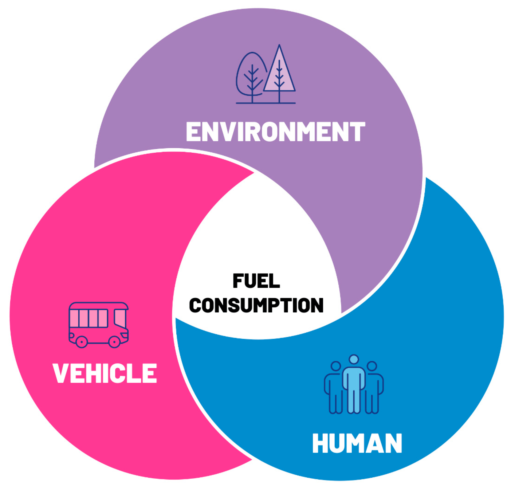
Figure 2.
General IFCAM application framework illustrating the transferability of the method across different vehicle types and operating sectors.
Figure 2.
General IFCAM application framework illustrating the transferability of the method across different vehicle types and operating sectors.
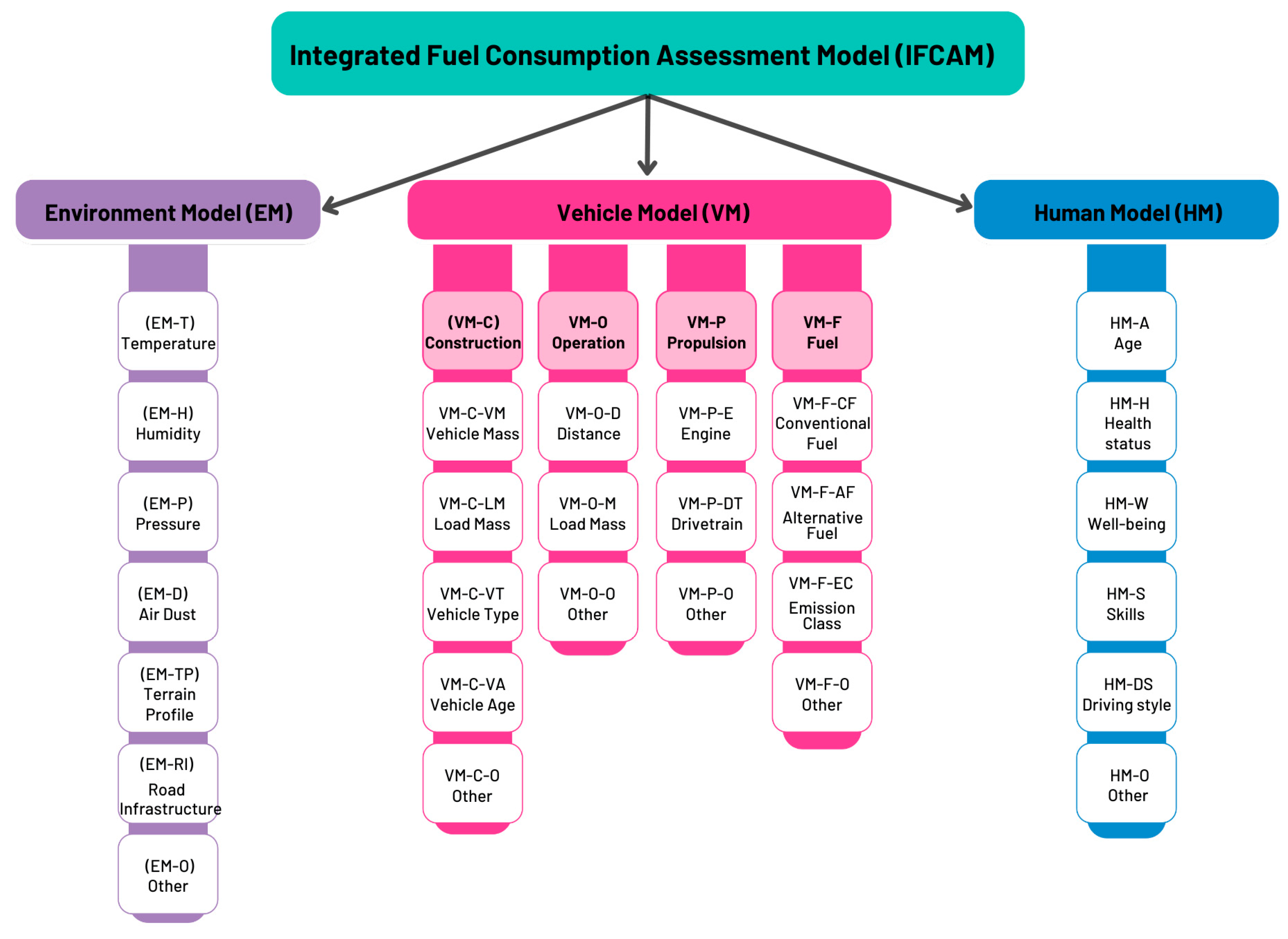
Figure 3.
General workflow of the Integrated Fuel Consumption Assessment Model (IFCAM), from system definition to model integration, decision-support and long-term monitoring.
Figure 3.
General workflow of the Integrated Fuel Consumption Assessment Model (IFCAM), from system definition to model integration, decision-support and long-term monitoring.
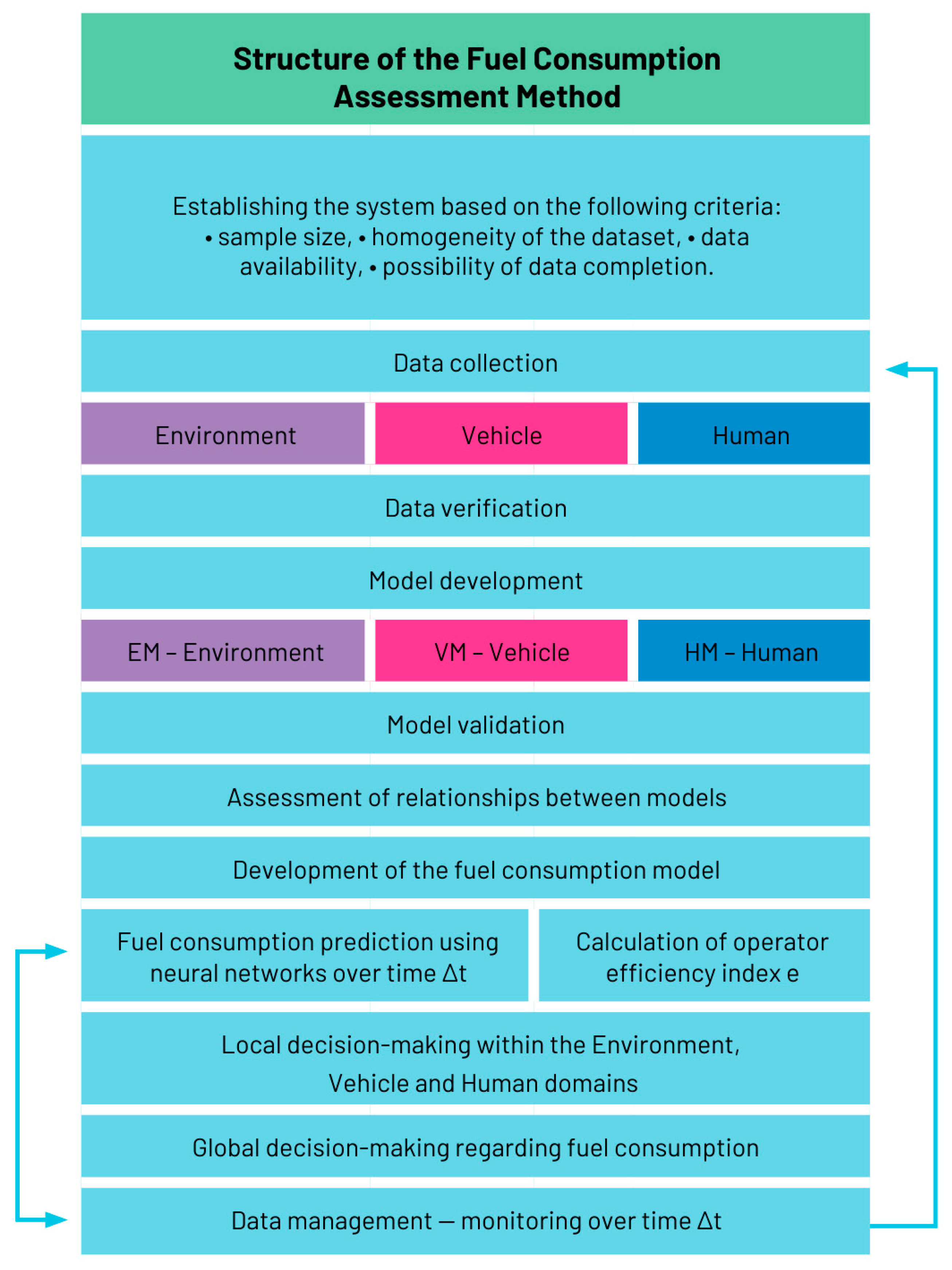
Figure 4.
Examples of LHD loader operation in the analysed underground mine: (a) loading and manoeuvring in a low-height drift under constrained visibility conditions; (b) loading of broken ore directly at the production face.
Figure 4.
Examples of LHD loader operation in the analysed underground mine: (a) loading and manoeuvring in a low-height drift under constrained visibility conditions; (b) loading of broken ore directly at the production face.
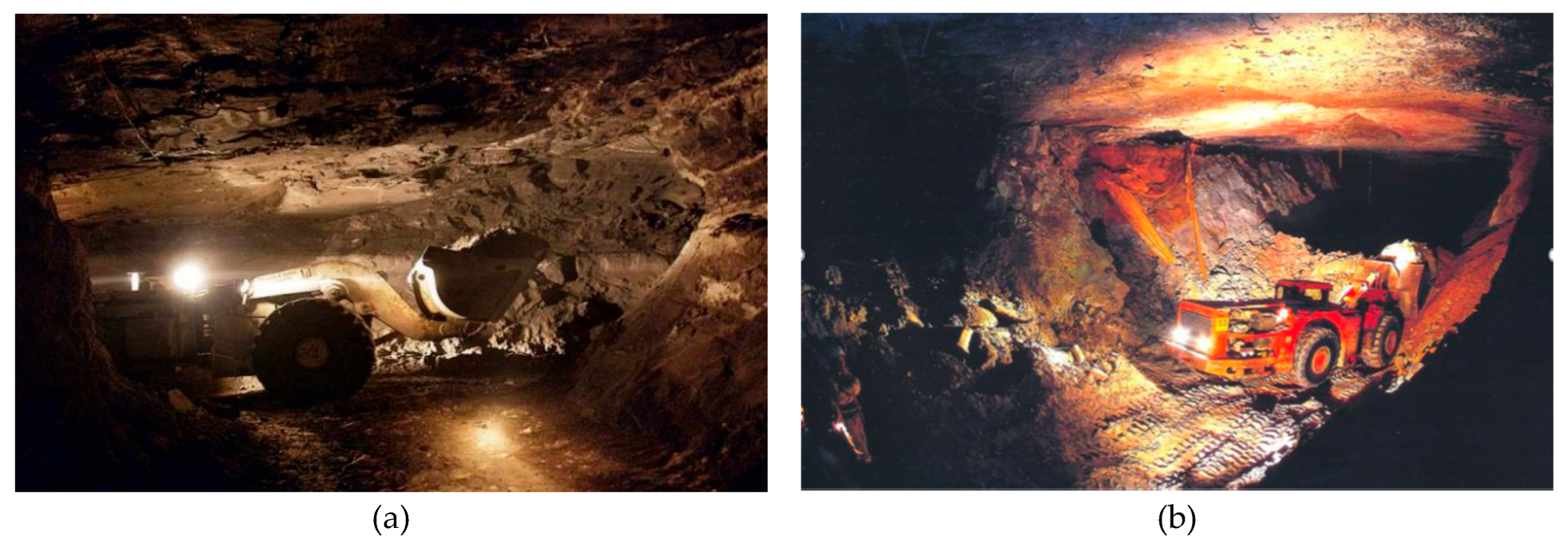
Figure 5.
Relationship between dry-bulb temperature (t_a) and the average hourly fuel consumption (HFC). The fitted second-order polynomial illustrates the moderate, non-linear influence of temperature on fuel demand, with a noticeable increase above approximately 36.5 °C. Pearson correlation: r = 0.20.
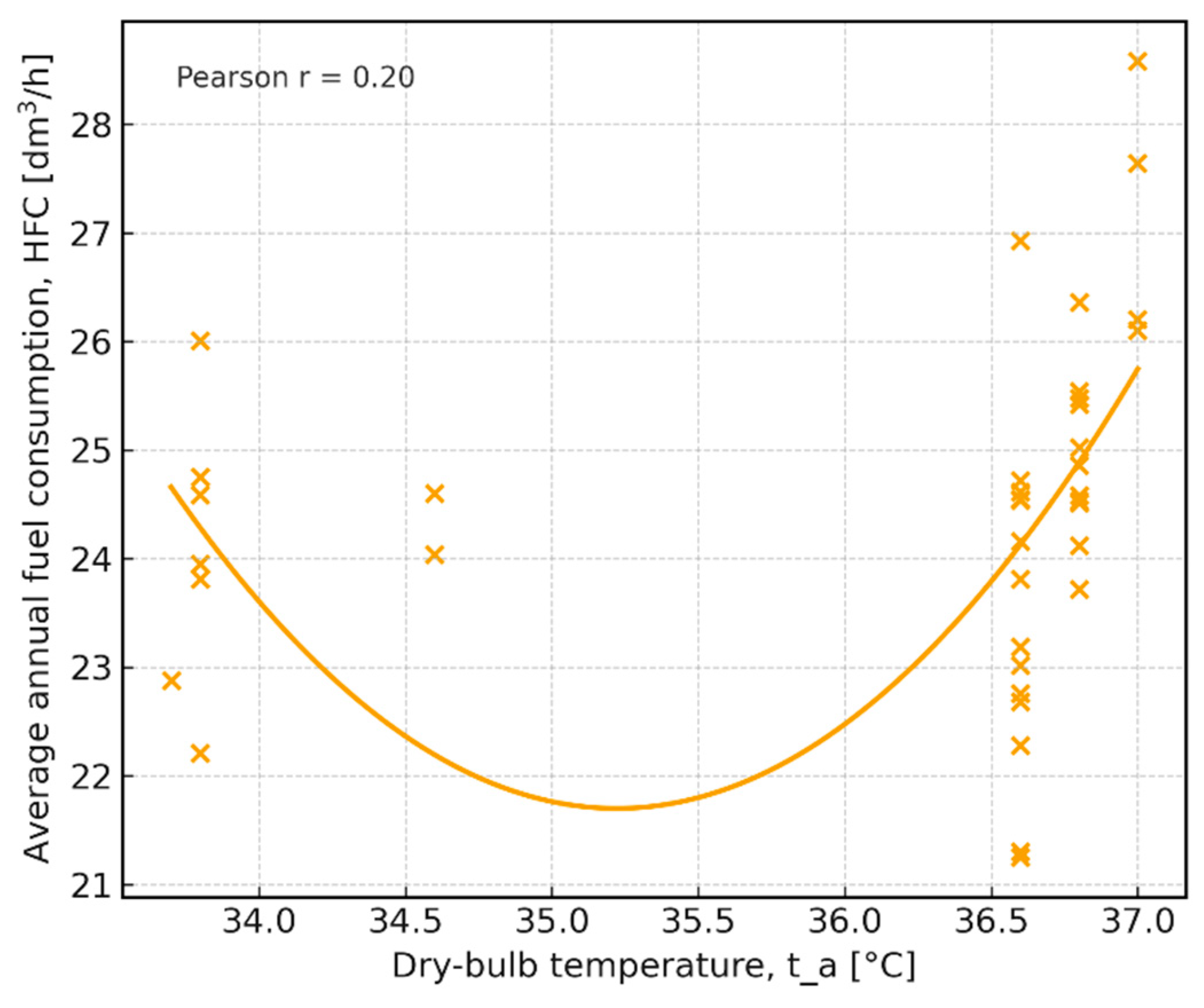
Figure 6.
Relationship between machine age and hourly fuel consumption (HFC). Spearman’s rank correlation (r = −0.17, p = 0.295) indicates no significant dependence; therefore machine age was not included as a predictive variable in the Vehicle Model.
Figure 6.
Relationship between machine age and hourly fuel consumption (HFC). Spearman’s rank correlation (r = −0.17, p = 0.295) indicates no significant dependence; therefore machine age was not included as a predictive variable in the Vehicle Model.
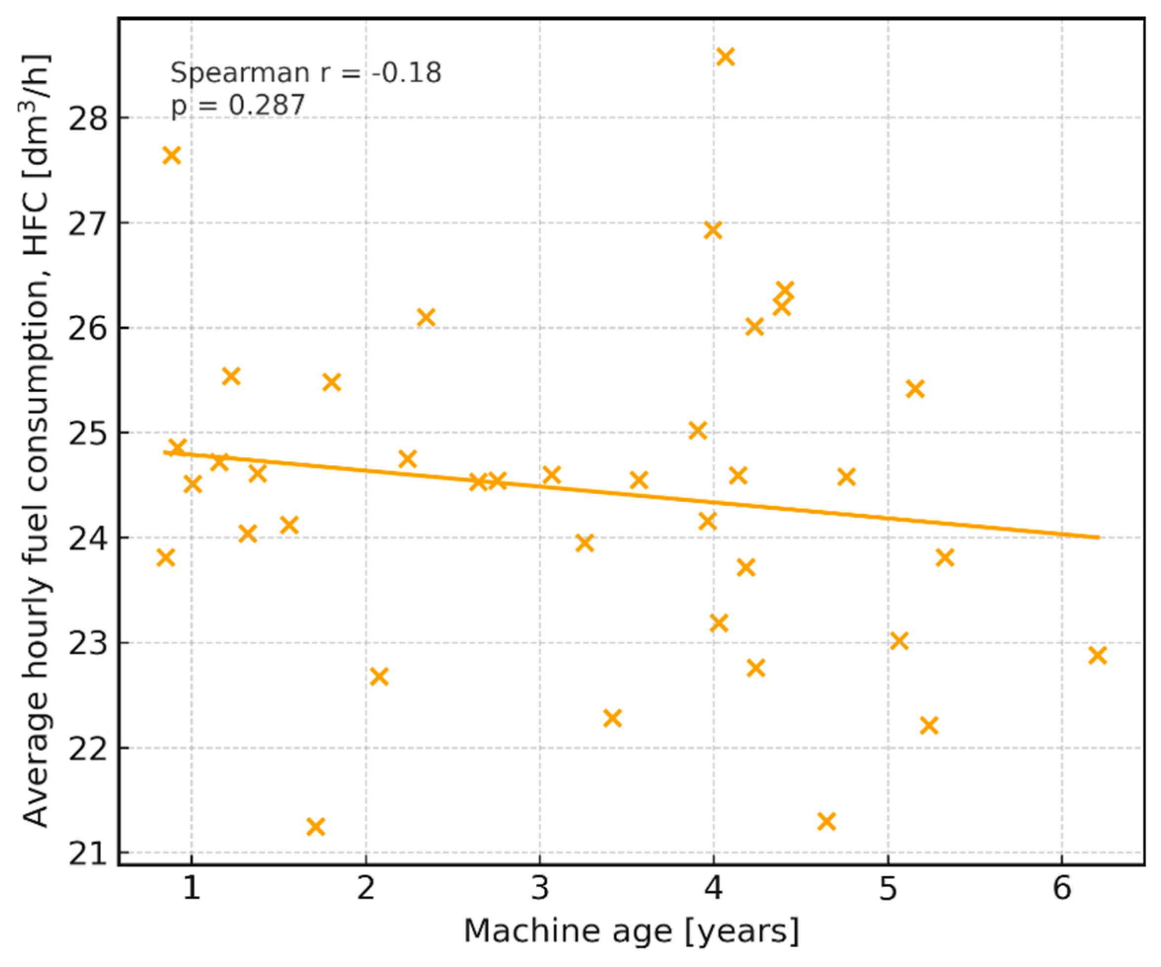
Figure 7.
Relationship between machine age and annual fuel consumption. Spearman’s rank correlation (r = −0.69, p < 0.001) indicates a strong negative monotonic association, showing that older machines consume less fuel annually because they are used less intensively.
Figure 7.
Relationship between machine age and annual fuel consumption. Spearman’s rank correlation (r = −0.69, p < 0.001) indicates a strong negative monotonic association, showing that older machines consume less fuel annually because they are used less intensively.
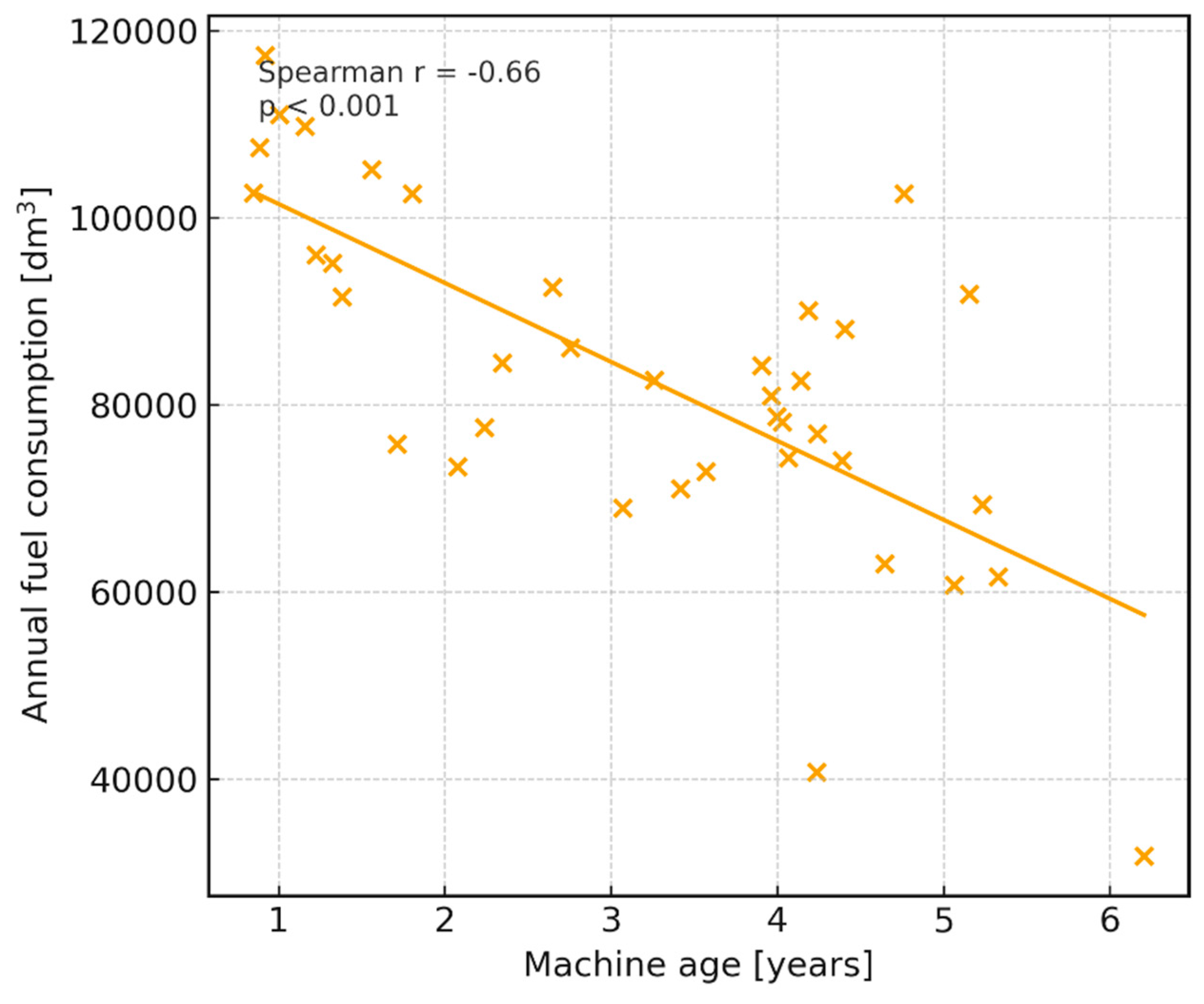
Figure 8.
Distribution of hourly fuel consumption (HFC) for all 38 machines across fourteen months (Nov 2020–Dec 2021).
Figure 8.
Distribution of hourly fuel consumption (HFC) for all 38 machines across fourteen months (Nov 2020–Dec 2021).
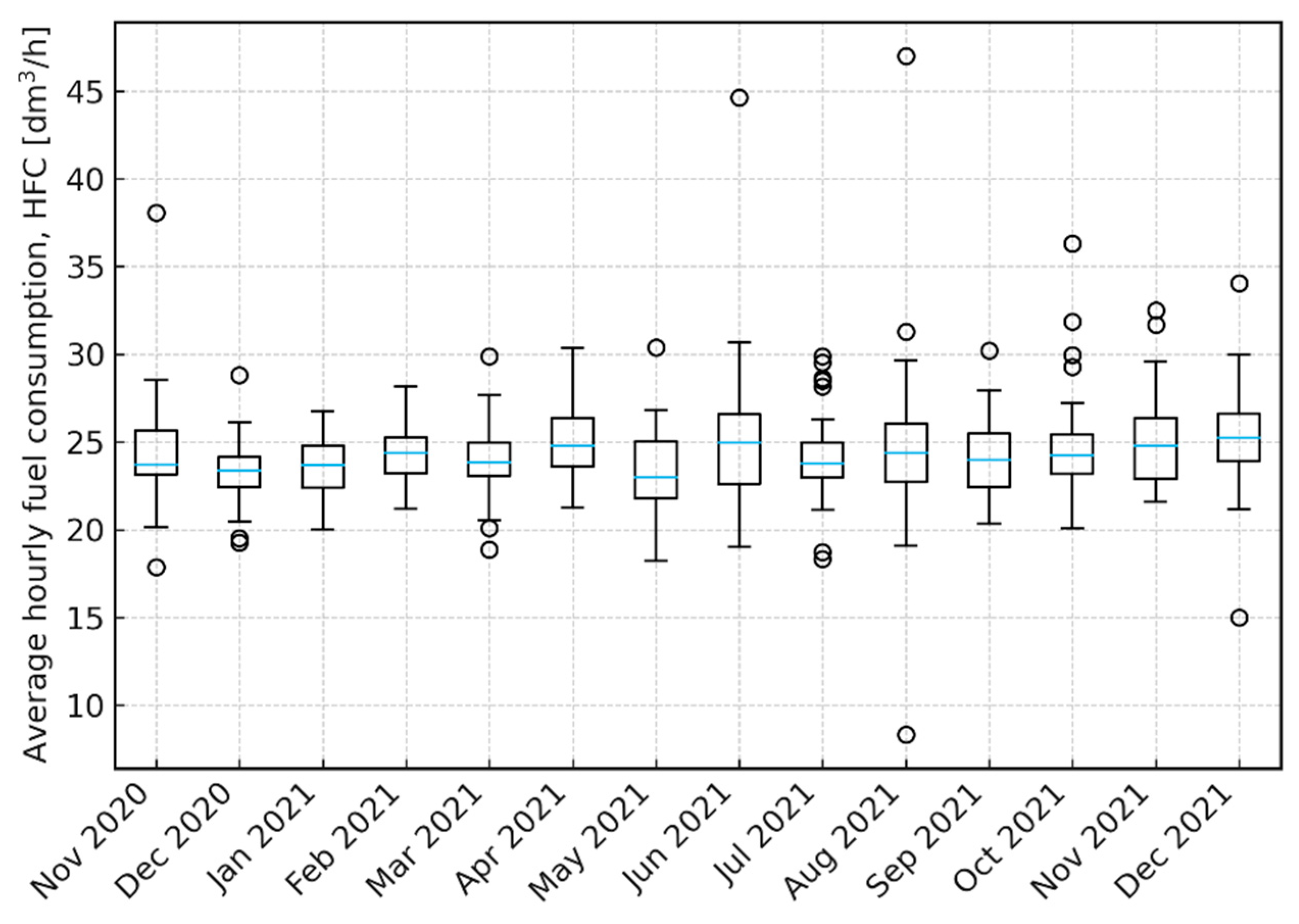
Figure 9.
Heat map of the engine operating distribution in the torque–speed domain, expressed as the relative frequency of occurrence [%].
Figure 9.
Heat map of the engine operating distribution in the torque–speed domain, expressed as the relative frequency of occurrence [%].
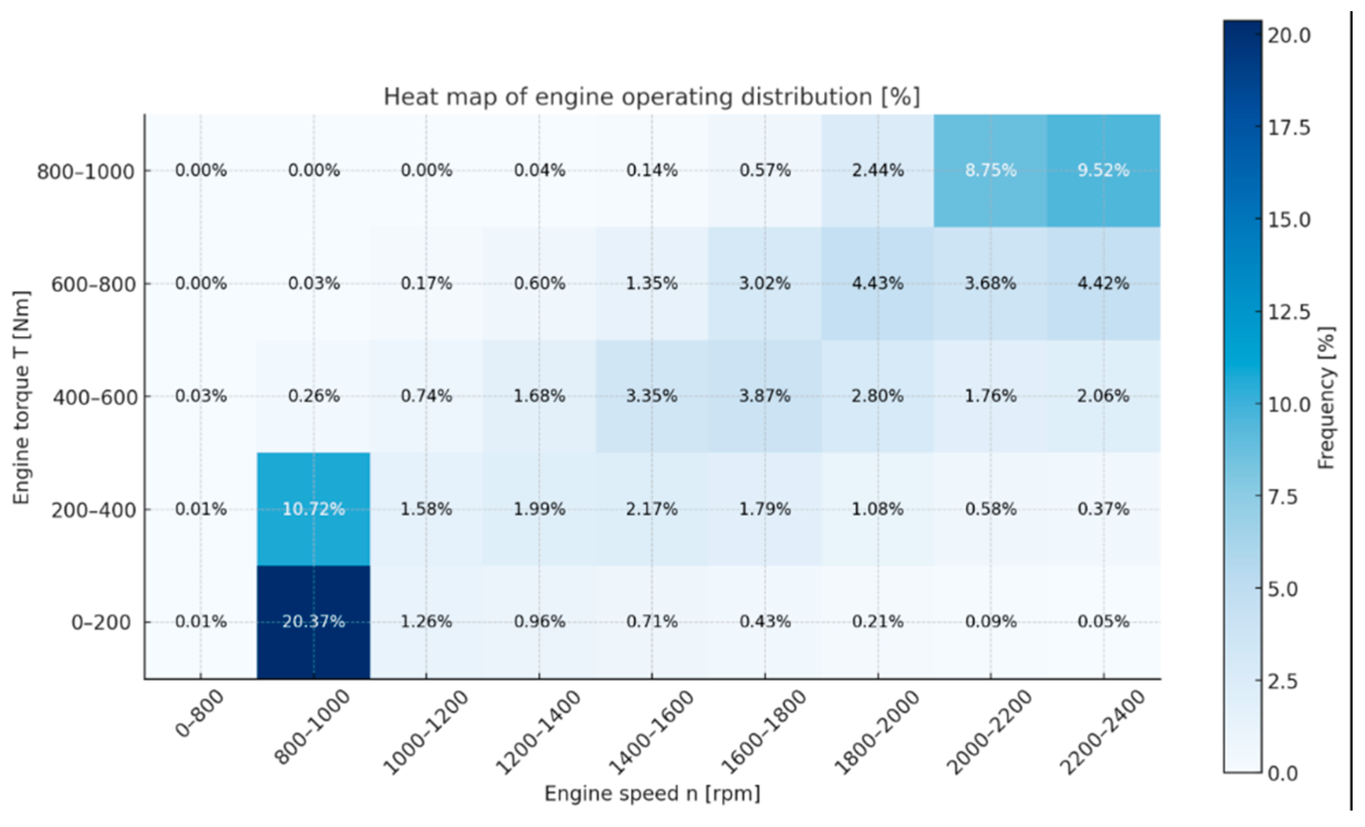
Figure 10.
Mean specific fuel consumption (SFC) for all operators. The dashed line represents the fleet-level reference value of 205 g/kWh used to identify operators with above-average and below-average fuel efficiency.
Figure 10.
Mean specific fuel consumption (SFC) for all operators. The dashed line represents the fleet-level reference value of 205 g/kWh used to identify operators with above-average and below-average fuel efficiency.
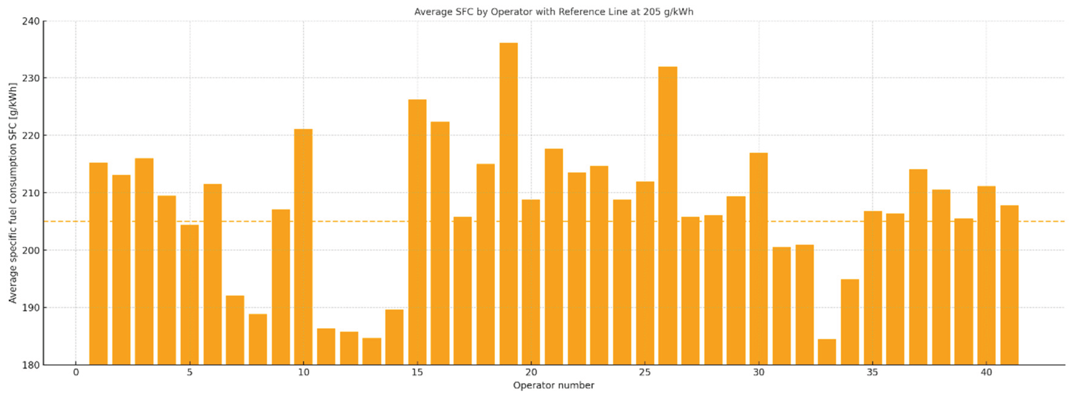

Table 1.
Summary of the key operational, environmental and data-acquisition parameters used in the IFCAM study.
Table 1.
Summary of the key operational, environmental and data-acquisition parameters used in the IFCAM study.
| Category | Value/Range | Description / Notes |
| Mining system | 3 underground mines | Total production capacity approx. 30–35 Mt/year |
| Mining depth | ~400–1200 m | Geothermal gradient ~1°C per 30–33 m |
| Temperature (dry-bulb) | 33–37°C | Daily measurements across 10+ districts |
| Climate substitute temperature | 29–31°C | Based on ta, tw, air velocity |
| Relative humidity | 85–95% | High and stable across districts |
| Dust level | High | Qualitative assessment from ventilation reports |
| Air velocity | 0–2 m/s | Depending on location and ventilation conditions |
| Roadway inclination | ≤5° | Horizontal drift system (room-and-pillar) |
| Roadway width / height | ≥4.6 m / 2–4 m | Height dependent on ore thickness |
| Total fleet | ~1200 units | Includes LHDs, haul trucks, drilling rigs etc. |
| LHD population | 123 units | Most numerous category |
| Selected LHD group | 45 units | Homogeneous class used for IFCAM validation |
| Annual fuel use of selected group | >4.1 million litres | Highest consumption in the fleet |
| Bucket capacity | ~4.5–5.0 m³ | Representative for selected class |
| Machine operating weight | ~28–30 t | Typical for the selected loaders |
| Operators included | 41 | All operators assigned to selected machines |
| Typical shift duration | ~6 h underground | Standard for the analysed group |
| Fuel-use variation between operators | 10–18% | Under identical working conditions |
| Sampling frequency | 1 Hz | Continuous recording of operational parameters |
| Number of parameters | >30 | Engine, drivetrain, hydraulics, process parameters |
| Cycle identification | 4 phases | Loading, loaded haul, dumping, empty return |
Disclaimer/Publisher’s Note: The statements, opinions and data contained in all publications are solely those of the individual author(s) and contributor(s) and not of MDPI and/or the editor(s). MDPI and/or the editor(s) disclaim responsibility for any injury to people or property resulting from any ideas, methods, instructions or products referred to in the content. |
© 2025 by the authors. Licensee MDPI, Basel, Switzerland. This article is an open access article distributed under the terms and conditions of the Creative Commons Attribution (CC BY) license (http://creativecommons.org/licenses/by/4.0/).
Copyright: This open access article is published under a Creative Commons CC BY 4.0 license, which permit the free download, distribution, and reuse, provided that the author and preprint are cited in any reuse.


