Decorated Loop-Spaces I: Foundations and Applications

1. Introduction

1.1. Motivation

Many processes of interest across almost every domain which humans have concerned themselves with are not perfectly periodical, but indeed quasi-periodical. For instance, in evolutionary biology, reproduction cannot be modelled as a simple cyclic process, because epigenetic modifications and mutations are introduced at the level of the individual.1 It therefore behooves us greatly to take these perturbations into account.

In topology, there is a simple tool for describing cyclic processes2, as given by the free loop-space $\mathcal{L}X$ of a space X. It is the set of all maps of the form:

$$\mathcal{L}X\mathrm{Maps}(S^1,X)$$

(1)

from the circle into X. While it is conceptually elegant, we do in fact have good motivation to tweak it, due to the reasons mentioned previously. However, because the original formulation is very clean as is, it would serve us not to alter it too drastically. Thus, we propose a conservative modification, called the decorated loop-space (DLS) of X, as follows:

$$\widehat{\mathcal{L}}X\mathrm{Maps}({\widehat{S}}^1,\widehat{X})$$

(2)

where we explicitly define ${\widehat{S}}^1$ to be equal to the union of $S^1$ with some additional datum ${\left\{g_j\right\}}_{j\in J}$, and $\widehat{X}$ is similarly defined as the union of X with some additional datum ${\left\{p_k\right\}}_{k\in K}$. After quick re-writing of Equation (2), we get:

$$\widehat{\mathcal{L}}\mathrm{Maps}(S^1,X)\times \prod _{j\in J}\mathrm{Maps}(\left\{g_j\right\},\widehat{X})$$

(3)

and we denote the right-hand-side (the decorator) by:

$$\mathfrak{D}=\prod _{j\in J}\mathrm{Maps}(\left\{g_j\right\},\widehat{X}).$$

(4)

In the case where $\left\{g_j\right\}$ is a single marked point, then our decorator reduces to:

$$\mathfrak{D}={\widehat{X}}^J$$

(5)

which is just the function space of J-indexed pro-objects in $\widehat{X}$. While we do eventually wish to move beyond this simple setup, it is enough for a toy model. This allows us to describe constraints, energies, boundary conditions, defects, mollifiers, or other kinds of “test data” as simple punctures along with a “natural" choice of image $p_k$, called a decoration.

The number of possible data we can model under this single paradigm is expected to be quite broad, although with the caveat that each case warrants a specialized treatment. We will not be able to cover every single application here, but we introduce the machinery along with a few conceptual examples to get the ball rolling, so to speak. This paper shall be a mixture of topological and categorical scaffolding, along with practical uses. We present many vantage points, at the cost of dissatisfying specialists in any one area.

1.2. Outline of the paper

Section 2 develops the basic formalism of decorated spaces and decorated loop-spaces. We introduce the category $\mathbf{DecLpSpc}$, distinguish carefully between decorators and connectors on functor categories, and construct the decorated loop functor $\widehat{\mathsf{\Omega }}$ together with a notion of decorated concatenation. We also discuss decorated suspension and a decorated Eckmann–Hilton operator, setting up the interaction between loop- and suspension-like constructions in the decorated setting.

Section 3 turns to homotopy operations. We recall the classical Whitehead product, then define decorated Whitehead products and their higher analogues, exhibiting decorated homotopy groups as carrying a quasi-Lie structure refined by decoration data. We prove functoriality and graded-Jacobi type relations, describe a symmetric monoidal structure on $\mathbf{DecLpSpc}$, and explain how operads act on decorated loop-spaces, leading to recognition results for iterated decorated loop functors ${\widehat{\mathsf{\Omega }}}^n$. A worked example on a wedge of spheres illustrates how decorations enrich a nontrivial Whitehead product.

Section 4 collects applications. We sketch how decorated loop-spaces package worldsheet geometry, background fluxes, and vacuum expectation values in string-theoretic settings; how decorations separate epigenetic from phenotypic data in a simple evolutionary model; and how connectors organise feedback, integral action, and signal-flow architectures in control-theoretic examples. We close with a brief discussion of future directions, including more systematic operadic refinements, computable invariants, and data-driven variants of the framework. The appendices contain additional case studies and technical remarks, including a signal-processing/OCR example and further comments on operadic and higher-algebraic extensions of the theory.

2. Categorical Considerations

2.1. The Category $\mathbf{DecLpSpc}$

Before developing decorated loop spaces and their adjunctions, we first clarify the categorical environment these constructions reside in. The category $\mathbf{DecLpSpc}$ is designed to refine the usual category of based topological spaces by enriching every object with puncture–data and every morphism with connector–data. This structure records how decorations are transported along continuous maps, and it ensures that subsequent constructions, such as decorated suspensions, decorated loop spaces, and the Eckmann–Hilton duality Section 2.3, are all implemented functorially. In particular, $\mathbf{DecLpSpc}$ serves as the ambient category in which the decorated analogues of classical homotopical operations naturally live.

Let us now formalize the category of decorated loop spaces (DLS).

Warning 1.

This construction applies specifically to the case in which the $\left\{g_j\right\}$ are (families of) points; slight modifications must be made to treat the other cases.

Throughout, let $S^n$ denote the n–sphere equipped with a fixed CW structure (used only to organize marked loci), and let P denote a fixed decoration parameter space.

Definition 1.

An object of $\mathbf{DecLpSpc}$ is a pair $(X,{\mathfrak{D}}_X)$ consisting of:

• a based topological space X, and
• a decoration functor

  $${\mathfrak{D}}_X:{\mathbf{Loop}}_X⟶\mathbf{Set}$$
  assigning to each loop $L:S^n\to X$ a set ${\mathfrak{D}}_X\left(L\right)$ of admissible decorations.

Warning 2.

The connectors introduced below should not be confused with the decorator. The decorator $\mathfrak{D}$ is responsible only for selecting the image of each generator $g_j$ in $\widehat{X}$; that is, it supplies a family of assignments

$$g_j⟼p_k\in \widehat{X}.$$

By contrast, the connectors act not on the generators themselves, but on the corresponding families of functions.

More precisely, for each generator $g_j$ decorated by $p_k$, we consider the functor categories

$$\mathrm{Fun}(g_j,\mathcal{C})\mathrm{and}\mathrm{Fun}(p_k,\mathcal{D}),$$

with $\mathcal{C}$ and $\mathcal{D}$ objects of the same ambient category. A connector is then a natural transformation

$${\phi }_{g_j}:\mathrm{Fun}(g_j,\mathcal{C})\Rightarrow \mathrm{Fun}(p_k,\mathcal{D}),$$

which transports families of functions associated to the mode $g_j$ into families indexed by the decorated image $p_k$. In this way, the decorator determines the target of each connector, while the connector itself acts at the level of function-families.

In the applications of this paper, the decoration functor is taken to be as in Equation (4) corresponding to a finite family of marked loci $\left\{g_j\right\}$ on the domain $S^n$; equivalently, these are pointwise labels or weights attached to the loop. We write

$$\widehat{\mathcal{L}}X:=\mathcal{L}X\times {\mathfrak{D}}_X\left(\mathcal{L}X\right)$$

for the associated decorated loop space.

Definition 2.

A morphism

$$(f,\phi ):(X,{\mathfrak{D}}_X)⟶(Y,{\mathfrak{D}}_Y)$$

in $\mathbf{DecLpSpc}$ consists of:

• a continuous map $f:X\to Y$, and
• a natural transformation (thedecoration connector)

  $$\phi :{\mathfrak{D}}_X⟹f^{*}{\mathfrak{D}}_Y,$$
  that is, for every loop $L:S^n\to X$ a function

  $${\phi }_L:{\mathfrak{D}}_X\left(L\right)⟶{\mathfrak{D}}_Y(f\circ L).$$

The connector $\phi$ prescribes how decorations flow along f; in physical practice it may encode trivial relabelings, screening or renormalization transformations, or the action of auxiliary symmetry data.

Definition 3.

Given composable morphisms

$$(X,{\mathfrak{D}}_X)\stackrel{(f,\phi )}{\to }(Y,{\mathfrak{D}}_Y)\stackrel{(g,\psi )}{\to }(Z,{\mathfrak{D}}_Z),$$

their composite is

$$(g,\psi )\circ (f,\phi ):=\left(g\circ f,\psi \circ \left(f^{*}\phi \right)\right),$$

i.e. the geometric part composes as usual, while the decoration connector is the composite

$${\mathfrak{D}}_X\left(L\right)\stackrel{{\phi }_L}{\to }{\mathfrak{D}}_Y(f\circ L)\stackrel{{\psi }_{f\circ L}}{\to }{\mathfrak{D}}_Z(g\circ f\circ L).$$

The identity morphism on $(X,{\mathfrak{D}}_X)$ is $({\mathrm{id}}_X,{\mathrm{id}}_{{\mathfrak{D}}_X})$.

Proposition 1.

The data above endows $\mathbf{DecLpSpc}$ with the structure of a category: composition is associative, and identity morphisms act as strict units.

Remark 1.

The forgetful functor

$$U:\mathbf{DecLpSpc}⟶\mathbf{Top},(X,{\mathfrak{D}}_X)⟼X,$$

admits a natural decorated loop space construction via $X\mapsto \widehat{L}X$, as described above.

2.2. The Decorated Suspension

The suspension functor plays a central role in the loop–suspension adjunction, and in the decorated setting it must be refined to incorporate connector–data. We begin with the classical construction. For any based space $(X,x_0)$, the reduced suspension $\Sigma X$ is obtained from $X\times I$ by collapsing

$$X\times \left\{0\right\}\sim {*}_{-},X\times \left\{1\right\}\sim {*}_{+},$$

where ${*}_{-}$ and ${*}_{+}$ are the south and north poles. The canonical pinch map

$${\nabla }_X:\Sigma X⟶S^1\wedge X$$

(6)

is the quotient identifying the two ends of the suspension as the two points of the circle. Equivalently, ${\nabla }_X$ collapses $X\times \left\{0\right\}$ and $X\times \left\{1\right\}$ to the two poles of $S^1$, and restricts to the identity on X along the equatorial region.

In the decorated setting, the suspension construction is augmented by the connector–data supplied by a decorated morphism. Given a decorated object $\widehat{X}=(X,\left\{p_i\right\})$ with punctures $\left\{p_i\right\}$ and a connector $\phi$ describing how punctures propagate under morphisms, we form the decorated suspension

$$\widehat{\Sigma }X\Sigma X\cup \mathrm{Maps}(\left\{g_j\right\},\left\{p_i\right\}),$$

where the connector–data are attached along the classical pinch map (6). Intuitively, $\widehat{\Sigma }X$ is obtained by suspending the underlying topological space while simultaneously transporting the puncture–data upward along the suspension cylinder, allowing decorations to “flow’’ between the poles under the control of $\phi$.

This decorated suspension is functorial in $\mathbf{DecLpSpc}$: a decorated morphism $(f,\phi ):\widehat{X}\to \widehat{Y}$ induces a uniquely determined morphism

$${(f,\phi )}_{\Sigma }:\widehat{\Sigma }X⟶\widehat{\Sigma }Y,$$

obtained by applying f to the underlying suspended space and applying $\phi$ to the connector–data. It is through this functoriality that the decorated loop–suspension adjunction of Section 2.3, and hence the decorated Eckmann–Hilton operator, becomes well-defined.

2.3. Eckmann–Hilton Duality

Classically, the loop–suspension adjunction asserts a natural isomorphism

$$\mathrm{Maps}(X,\mathsf{\Omega }Y)\cong \mathrm{Maps}(\Sigma X,Y),$$

(7)

often referred to as the Eckmann–Hilton duality. This relationship expresses the fact that based maps into a loop space are equivalent to suspended maps into the underlying space; see, for example, [14,20], and [16] for a more informal retrospective.3

In our decorated setting, where every object carries auxiliary puncture–data and every morphism $(f,\phi )$ consists of an underlying continuous map together with a connector specified as in Definition 2, this adjunction persists in a fully functorial manner. Namely, the based decorated loop space is defined by

$$\widehat{\mathsf{\Omega }}X{\mathrm{Maps}}_{*}\left({\widehat{S}}^1,\widehat{X}\right),$$

(with basepoint *) and the decorated suspension $\widehat{\Sigma }X$ is obtained by freely adjoining the connector–data along the suspension pinch map, as described in Section 2.2. With these definitions in place, we obtain the decorated adjunction

$$\mathrm{Maps}(\widehat{X},\widehat{\mathsf{\Omega }}Y)\cong \mathrm{Maps}(\widehat{\Sigma }X,\widehat{Y}),$$

(8)

and every decorated morphism

$$(f,\phi ):\widehat{X}⟶\widehat{Y}$$

determines a uniquely associated decorated suspension adjoint

$${(f,\phi )}_{♭}:\widehat{\Sigma }X⟶\widehat{Y}.$$

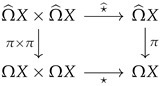
Following the classical pattern, we define the decorated Eckmann–Hilton operator by looping this adjoint:

$$\widehat{\mathcal{EH}}(f,\phi )\mathsf{\Omega }\left({(f,\phi )}_{♭}\right):\mathsf{\Omega }\widehat{\Sigma }X⟶\mathsf{\Omega }\widehat{Y}.$$

(9)

This construction has the advantage of being both fully typed and functorial: $\widehat{\mathcal{EH}}(f,\phi )$ is a well-defined morphism in the category $\mathbf{DecLpSpc}$, and reduces to the classical $\mathsf{\Omega }\Sigma$-construction when all decorations are trivial. In particular, (9) constitutes the correct decorated analogue of composing a map with the $\mathsf{\Omega }\Sigma$-shift in the ordinary Eckmann–Hilton duality.

Proposition 2

(Decorative Functoriality). Let $\widehat{X},\widehat{Y},\widehat{Z}$ be objects of $\mathbf{DecLpSpc}$ and let

$$(f,\phi ):\widehat{X}⟶\widehat{Y},(g,\psi ):\widehat{Y}⟶\widehat{Z}$$

be decorated morphisms. The assignment

$$(f,\phi )⟼\widehat{\mathcal{EH}}(f,\phi )=\mathsf{\Omega }\left({(f,\phi )}_{♭}\right):\mathsf{\Omega }\widehat{\Sigma }X⟶\mathsf{\Omega }\widehat{Y}$$

defines a functorial operation on decorated morphisms. Concretely:

• $\widehat{\mathcal{EH}}\left({\mathrm{id}}_{\widehat{X}}\right)={\mathrm{id}}_{\mathsf{\Omega }\widehat{\Sigma }X}.$
• $\widehat{\mathcal{EH}}\left((g,\psi )\circ (f,\phi )\right)=\widehat{\mathcal{EH}}(g,\psi )\circ \widehat{\mathcal{EH}}(f,\phi ).$

Proof. 

We use two facts: the naturality (functoriality) of the loop–suspension adjunction

$$\mathrm{Maps}(\widehat{X},\widehat{\mathsf{\Omega }}Y)\cong \mathrm{Maps}(\widehat{\Sigma }X,\widehat{Y}),$$

and the fact that $\mathsf{\Omega }$ is a functor on $\mathbf{DecLpSpc}$.

(1) Identity. The identity morphism ${\mathrm{id}}_{\widehat{X}}$ transposes under the adjunction to the identity ${\left({\mathrm{id}}_{\widehat{X}}\right)}_{♭}={\mathrm{id}}_{\widehat{\Sigma }X}$. Applying $\mathsf{\Omega }$ yields

$$\widehat{\mathcal{EH}}\left({\mathrm{id}}_{\widehat{X}}\right)=\mathsf{\Omega }\left({\left({\mathrm{id}}_{\widehat{X}}\right)}_{♭}\right)=\mathsf{\Omega }\left({\mathrm{id}}_{\widehat{\Sigma }X}\right)={\mathrm{id}}_{\mathsf{\Omega }\widehat{\Sigma }X},$$

as required.

(2) Composition. Consider the composite $(g,\psi )\circ (f,\phi ):\widehat{X}\to \widehat{Z}$. By naturality of the adjunction (the transposition isomorphism is natural in both variables), the suspension adjoint of the composite equals the composite of the suspension adjoints up to the evident structural maps coming from $\Sigma$; schematically,

$${\left((g,\psi )\circ (f,\phi )\right)}_{♭}={(g,\psi )}_{♭}\circ \widehat{\Sigma }\left({(f,\phi )}_{♭}\right),$$

where $\widehat{\Sigma }$ denotes the decorated suspension functor and the right-hand composition is the ordinary composition of maps $\widehat{\Sigma }X\to \widehat{Z}$. Applying the functor $\mathsf{\Omega }$ (which preserves composition) yields

$$\widehat{\mathcal{EH}}\left((g,\psi )\circ (f,\phi )\right)=\mathsf{\Omega }\left({(g,\psi )}_{♭}\circ \widehat{\Sigma }\left({(f,\phi )}_{♭}\right)\right)=\mathsf{\Omega }\left({(g,\psi )}_{♭}\right)\circ \mathsf{\Omega }\left(\widehat{\Sigma }\left({(f,\phi )}_{♭}\right)\right).$$

Because $\mathsf{\Omega }$ and $\widehat{\Sigma }$ are adjoint functors, the latter composition is equal (under the canonical identifications afforded by the adjunction) to

$$\mathsf{\Omega }\left({(g,\psi )}_{♭}\right)\circ \mathsf{\Omega }\left({(f,\phi )}_{♭}\right)=\widehat{\mathcal{EH}}(g,\psi )\circ \widehat{\mathcal{EH}}(f,\phi ).$$

Thus the assignment preserves composition, completing the proof.    □

2.4. Heteromorphisms

Definition 4

(Heteromorphism). Let $\mathcal{C}$ and $\mathcal{D}$ be categories. A heteromorphism (or chimera morphism) from an object $A\in \mathcal{C}$ to an object $B\in \mathcal{D}$ consists of the following data:

• an ambient category$\mathcal{E}$ together with (not necessarily essentially unique) functors

  $$J_{\mathcal{C}}:\mathcal{C}⟶\mathcal{E},J_{\mathcal{D}}:\mathcal{D}⟶\mathcal{E},$$
  which we think of as embeddings of $\mathcal{C}$ and $\mathcal{D}$ into a common environment;
• a morphism in $\mathcal{E}$

  $$f:J_{\mathcal{C}}\left(A\right)⟶J_{\mathcal{D}}\left(B\right).$$

We write

$$A⇝B$$

for such a heteromorphism, and denote the set of all heteromorphisms from A to B by

$$\mathrm{Het}(A,B):={\mathrm{Hom}}_{\mathcal{E}}\left(J_{\mathcal{C}}\left(A\right),J_{\mathcal{D}}\left(B\right)\right).$$

Thus a heteromorphism $A⇝B$ is, in particular,

• a morphism $A\to B$ whose domain and codomain lie in different categories$\mathcal{C}$ and $\mathcal{D}$, and
• a morphism taking place inside a single ambient category$\mathcal{E}$ which contains (the images of) both $\mathcal{C}$ and $\mathcal{D}$.

Remark 2.

Fixing $\mathcal{C}$, $\mathcal{D}$ and $\mathcal{E}$ as in Definition 4, the assignment

$$\mathrm{Het}:{\mathcal{C}}^{\mathrm{op}}\times \mathcal{D}⟶\mathrm{Set},(A,B)⟼{\mathrm{Hom}}_{\mathcal{E}}\left(J_{\mathcal{C}}\left(A\right),J_{\mathcal{D}}\left(B\right)\right),$$

is a het-bifunctor in the sense of Ellerman: morphisms in $\mathcal{C}$ and $\mathcal{D}$ act on the left and right by pre- and postcomposition inside $\mathcal{E}$. This recovers the abstract $\mathrm{Het}$-formalism from a concrete ambient-category picture.4

Example 1.

As a first concrete class of heteromorphisms, it is useful to place a “semantic layer5” on top of $\mathbf{DecLpSpc}$. Let $\mathcal{N}$ be a category of narrative states, whose objects record coarse dynamical behaviours (for instance: stable equilibrium, damped oscillation, runaway growth, or an Ω-like nonterminating loop), and whose morphisms encode refinements or coarsegrainings between such descriptions. A semantic decoration functor is a functor

$$B:\mathbf{DecLpSpc}⟶\mathcal{N}$$

which assigns to each decorated space $(X,\mathcal{D})$ an abstract narrative $B(X,\mathcal{D})$ and to each morphism $F:(X,\mathcal{D})\to (Y,\mathcal{E})$ a corresponding update $B\left(F\right):B(X,\mathcal{D})\to B(Y,\mathcal{E})$. In the sense of Definition 4, taking the ambient category $\mathcal{E}=\mathcal{N}$ means that heteromorphisms out of $(X,\mathcal{D})$ into the semantic layer are simply arrows

$$\mathrm{Het}\left((X,\mathcal{D}),N\right)\cong {\mathrm{Hom}}_{\mathcal{N}}\left(B(X,\mathcal{D}),N\right),$$

so that higher homotopical operations on $\widehat{\mathsf{\Omega }}X$ (concatenation, suspension, decorated Whitehead products, and so on) induce systematic narrative operations (iteration, amplification, coarsegraining) on $B(X,\mathcal{D})$. This point of view will be exploited in the applications below, where we use B to track whether a given decorated feedback loop is genuinely terminating, stabilizing, or exhibits Ω-like nontermination.

3. Homotopical and Algebraic Structures on $\mathbf{DecLpSpc}$

The preceding sections developed the basic categorical framework for decorated loop spaces, together with their duality properties and suspension–pinch interactions. We now turn to the deeper structural layer that makes the category $\mathbf{DecLpSpc}$ a natural receptacle for both algebraic and homotopical data. Whereas the previous section emphasized the formal aspects of decorated loops (objects, morphisms, and elementary constructions); our goal here is to expose the rich network of higher coherences that decorate these loops at the level of homotopy.

The fundamental observation guiding this section is that decorated loops inherit more than a mere concatenation operation: they possess a family of homotopically meaningful compositions, each mediated by the decorating data. This leads to higher associativity conditions, generalized Eckmann–Hilton phenomena, and the emergence of structures reminiscent of $A_{\infty }$- and $E_{\infty }$-algebras. These can be understood as “hidden symmetries” arising from the compatibility between geometric gluing of loops and the combinatorics of their decorations. In this sense, $\mathbf{DecLpSpc}$ behaves simultaneously like an ordinary category, a monoidal category, and an operad—depending on which piece of data one chooses to foreground.

A second theme is the functoriality of decorated loop operations with respect to the underlying manifold or ambient space. Even though the loops themselves live in $\mathsf{\Omega }X$ or $LX$, the decorating data often lives in an auxiliary category: bundles, coefficient systems, local functionals, or even actions of a higher group or higher algebra. This interplay confers additional algebraic structure, sometimes in the form of convolution products and sometimes as transfer maps or regulators. As a result, the homotopical structure of $\mathbf{DecLpSpc}$ carries a blend of geometric and algebraic information encoded functorially.

Finally, the constructions in this section serve as the foundational layer for all later analytical and dynamical applications. The phenomena studied here (higher homotopies, coherence laws, operadic composition, and generalized concatenation) are precisely the mechanisms by which decorated loops interact with spectral data, transfer operators, and cyclic dynamical systems. The remainder of the paper will draw repeatedly on the structures introduced below, making this section a kind of “homotopical engine room’’ for the theory.

3.1. Concatenation, Higher Homotopies, and Coherence Laws

3.1.1. Classical Concatenation

Now that we have at least some picture in mind for the DLS construction, it is important to ensure it is actually a workable one. Probably the most important thing for us now is to define a notion of concatenation of loops in a DLS. Let’s first start with the usual notion of concatenation. Let $(X,x_0)$ be a space with base-point $x_0$ and $\mathsf{\Omega }X$ the based loop space defined by replacing the free-loops functor $\mathcal{L}$ in 1 with $\mathsf{\Omega }$. Specific maps are given by

$$\gamma :[0,1]⟶X\gamma \left(0\right)=x_0=\gamma \left(1\right)$$

(10)

Definition 5.

For $\alpha ,\beta \in \mathsf{\Omega }X$, concatenation of loops $\alpha ★\beta \in \mathsf{\Omega }X$ is given by

$$(\alpha ★\beta )\left[t\right]=\left\{\begin{array}{c}\alpha \left(2t\right)\mathrm{if}0\le t\le {\displaystyle \frac{1}{2}}\hfill \\ \beta (2t-1)\mathrm{if}{\displaystyle \frac{1}{2}}\le t\le 1\hfill \end{array}\right.$$

giving us a continuous map $★:\mathsf{\Omega }X\times \mathsf{\Omega }X\to \mathsf{\Omega }X$ with the constant loop $e\left(t\right)$ playing the role of a unit element.

3.1.2. Decorated Concatenation

What we want now is a modification of Definition 5 which extends to the DLS picture as painlessly as possible. That is, we want a continuous map:

$$\widehat{★}:\widehat{\mathsf{\Omega }}X\times \widehat{\mathsf{\Omega }}X\to \widehat{\mathsf{\Omega }}X$$

which reduces to ★ on the underlying based loops, while simultaneously gluing the appropriate decorating data. Our essential principle is that decorated loops $(\gamma ,\phi )$ ought to consist of ordinary loops $\gamma \in \mathsf{\Omega }X$ together with decorating data $\phi$ assigned along $\gamma$. Concatenation should combine these components by:

• Performing the usual piecewise-linear reparameterization on the geometric component
• Gluing the decorations along the pinch point in a manner compatible with decoration fibration.

The fibration is:

$$\pi :\widehat{\mathsf{\Omega }}X⟶\mathsf{\Omega }X$$

and the concatenation $\widehat{★}$ should be a lift of the classical concatenation along $\pi$.

Definition 6

(Decorated Concatenation). Let $(\alpha ,{\phi }_1),(\beta ,{\phi }_2)\in \widehat{\mathsf{\Omega }}X$ be decorated loops satisfying the usual compatibility conditions given in Equation 10. Theirdecorated concatenation

$$(\alpha ,{\phi }_1)★(\beta ,{\phi }_2)$$

is the decorated loop defined by

$$(\alpha ,{\phi }_1)★(\beta ,{\phi }_2)(\alpha ★\beta ,{\phi }_1{★}_{\mathrm{gl}}{\phi }_2)$$

where:

• $\alpha ★\beta$ is the usual concatenation from Definition 5;
• ${\phi }_1{★}_{\mathrm{gl}}{\phi }_2$ is the glued decoration obtained by pulling back ${\phi }_1$ and ${\phi }_2$ along the two halves of $[0,1]$ and identifying their endpoint values via the universal property of the pushout diagram

  $$S^1⟵\left\{1\right\}⟶S^1$$

This construction yields the continuous map $\widehat{★}$ which makes the diagram:

commute.

3.1.3. Coherence

In general, the operations ★ and $\widehat{★}$ are not strictly associative. Let $(\alpha ★\beta )★\gamma$ and $\alpha ★(\beta ★\gamma )$ be maps $[0,1]\to X$. Then, they traverse the same three loops but with different speeds/parameterizations. Thus, they are equal only up to homotopy, and there is in fact a canonical based homotopy between them built by “redistributing" the time intervals on $[0,1]$.

Proposition 3

(Functoriality of Decorated Concatenation). Let $F:(X,\mathcal{D})\to (Y,\mathcal{E})$ be a morphism of decorated spaces in the sense of Definition 2. Then the induced map

$$\widehat{\mathsf{\Omega }}F:\widehat{\mathsf{\Omega }}X⟶\widehat{\mathsf{\Omega }}Y$$

preserves decorated concatenation up to canonical homotopy. That is, for all decorated loops $({\gamma }_1,{\phi }_1),({\gamma }_2,{\phi }_2)\in \widehat{\mathsf{\Omega }}X$,

$$\widehat{\mathsf{\Omega }}F\left(({\gamma }_1,{\phi }_1)\widehat{★}({\gamma }_2,{\phi }_2)\right)\simeq \widehat{\mathsf{\Omega }}F({\gamma }_1,{\phi }_1)\widehat{★}\widehat{\mathsf{\Omega }}F({\gamma }_2,{\phi }_2).$$

Proof. 

On the level of underlying loops, functoriality of classical concatenation gives

$$F({\gamma }_1★{\gamma }_2)=F{\gamma }_1★F{\gamma }_2,$$

so the geometric component of the decorated concatenation is preserved strictly.

For decorations, recall that $\widehat{\mathsf{\Omega }}X$ and $\widehat{\mathsf{\Omega }}Y$ are defined via decoration fibrations

$${\pi }_X:\widehat{\mathsf{\Omega }}X⟶\mathsf{\Omega }X,{\pi }_Y:\widehat{\mathsf{\Omega }}Y⟶\mathsf{\Omega }Y.$$

Since F is a morphism in $\mathbf{DecLpSpc}$, it induces fiberwise maps

$$F_{*}:{\pi }_X^{-1}\left(\gamma \right)⟶{\pi }_Y^{-1}\left(F\gamma \right)$$

compatible with the gluing structure used to form decorated concatenation. In particular, if

$$({\gamma }_i,{\phi }_i)\in \widehat{\mathsf{\Omega }}X,i=1,2,$$

then decoration gluing satisfies

$$F_{*}\left({\phi }_1{★}_{\mathrm{gl}}{\phi }_2\right)\simeq F_{*}\left({\phi }_1\right){★}_{\mathrm{gl}}{F}_{*}\left({\phi }_2\right),$$

where the homotopy is induced by naturality of the gluing operations along the pushout diagram

$$S^1⟵\left\{1\right\}⟶S^1.$$

Finally, the classical associativity homotopy

$$({\gamma }_1★{\gamma }_2)★{\gamma }_3\simeq {\gamma }_1★({\gamma }_2★{\gamma }_3)$$

is natural with respect to F, and hence induces the required homotopy on the decorations through the fiberwise maps $F_{*}$. Putting these together yields a canonical homotopy

$$\widehat{\mathsf{\Omega }}F\left(({\gamma }_1,{\phi }_1)\widehat{★}({\gamma }_2,{\phi }_2)\right)\simeq \widehat{\mathsf{\Omega }}F({\gamma }_1,{\phi }_1)\widehat{★}\widehat{\mathsf{\Omega }}F({\gamma }_2,{\phi }_2),$$

completing the proof.    □

Remark 3.

Further, the unit $e★\alpha$ is only a unit up to homotopy;:

$$e★\alpha \simeq \alpha \simeq \alpha ★e$$

because extra time is spent at the basepoint.

This motivates one of the most important concepts we will need, owed to Stasheff. The idea itself is schematically very-simple:

Definition 7.

An $A_n$-space is a collection ofcoherentmaps:

$$m_k:{\mathcal{K}}_k\times X^k$$

(11)

with ${\mathcal{K}}_k$ a $(k-2)$-dimensional associahedron, $X^k$ a k-dimensional space, all satisfying $2\le k\le n$.

This immediately feeds into our next definition. Let A be an $A_n$-space. Then:

Definition 8.

An $A_{\infty }$-algebra structure on A is again a coherent set of maps:

$$m_k:A^{\otimes k}\to A$$

(12)

of degree $k-2$.

Of course, we have begun to brush up against the prickly issue of “coherence." The high-level idea is to allow for associativity (up to homotopy) at all levels. Stasheff himself [24] defined it using a convoluted but concise formula:

$$0=\sum _{i+j=n+1}\sum _{k=1}\pm m_i\left(a_1\otimes \dots \otimes a_{k-1}\otimes m_j(a_k\otimes \dots \otimes a_{k+j-1})\otimes a_{k+j}\dots \otimes a_n\right)$$

(13)

It is better if we just use an illustrative example. Consider the case of $n=3$. The identity becomes:

$$\begin{array}{c}\hfill m_1\left(m_3(a_1,a_2,a_3)\right)+\\ \hfill m_2(m_2(a_1,a_2),a_3)+m_2(a_1,m_2(a_2,a_3))+\\ \hfill m_3(m_1\left(a_1\right),a_2,a_3)+m_3(a_1,m_1\left(a_2\right),a_3)+m_3(a_1,a_2,m_1\left(a_3\right))\\ \hfill =0\end{array}$$

Formulated this way, things become much more manageable. Breaking it down, $m_1$ is a differential satisfying $m_1^2=0$, $m_2$ is a product (associative up to $m_3$), $m_3$ is a homotopy measuring the failure of associativity, and the $m_{>3}$ are higher homotopies which enforce the coherence among previous ones. An $A_{\infty }$-space obeying the structure of Equation (13) for $n\to \infty$.

The immediate reason to care about these structures is because any topological space which both admits an $A_{\infty }$-structure and whose connected components are homotopy-equivalent are precisely homotopy-equivalent to a loop-space. This has been known since at least the 1970s6, and reveals a deeper structure beyond the category we have presented here. In particular, this suggests that suitably grouplike decorated $A_{\infty }$-structures should be viewed as decorated loop-spaces, a perspective that will underly Section 3.1.2 and Section 3.2.

3.2. Decorated Whitehead Products and Homotopy Brackets

The story we have portrayed thus far is deceptively simple. The classical Whitehead product provides the first genuinely nontrivial binary operation in higher homotopy, measuring the obstruction to commuting two sphere families in a space. In the decorated setting, this operation arises naturally once we recognize that concatenation of decorated loops is homotopy–coherent rather than strictly functorial. When two decorated families interact, their underlying homotopies and their decoration data can interfere in a way not captured by ordinary loop composition. The decorated Whitehead product introduced in this section encodes precisely this second-order interaction: it refines the classical Whitehead bracket by incorporating the geometric information carried by decorations, and serves as the first layer in the higher $L_{\infty }$-type structure of the decorated loop space.

3.2.1. Classical Whitehead Products and Quasi-Lie Structure

Recall that our sphere $S^n$ comes with a CW-structure used to organized marked loci. CW-complexes are very nice spaces to work with.

Let $S^p$ and $S^q$ be a p-sphere and a q-sphere, respectively.7 Then, we can form a subspace of $S^p\times S^q$ by $S^p\vee S^q$, the wedge-sum (one–point union) of the spheres. Our CW-structure allows us to form attaching maps

$$a_{p,q}:S^{p+q-1}⟶S^p\vee S^q$$

of the unique $(p+q)$–cell in $S^p\times S^q$.

Definition 9

(Whitehead Product). Now, let $f:S^p\to X$ and $h:S^q\to X$ be based maps. Their composition is given by:

$$[f,g]=(f\vee g)\circ a_{p,q}:S^{p+q-1}⟶X$$

and is known as the Whitehead product.

These products were first investigated by Whitehead himself in [26], and many properties were immediately deduced. They are as follows; let $p,q,r\ge 2$. For $\alpha ,{\alpha }^{\prime }\in {\pi }_p\left(X\right)$ (the pth homotopy group of X), $\beta ,{\beta }^{\prime }\in {\pi }_q\left(X\right)$ and $\gamma \in {\pi }_r\left(X\right)$, Whitehead products satisfy:

• (identity) $[\alpha ,0]=0$ and $[0,\beta ]=0$.
• (bilinearity) $[\alpha +{\alpha }^{\prime },\beta ]=[\alpha ,\beta ]+[{\alpha }^{\prime },\beta ]$ and $[\alpha ,\beta +{\beta }^{\prime }]=[\alpha ,\beta ]+[\alpha ,{\beta }^{\prime }]$
• (graded symmetry) $[\alpha ,\beta ]={(-1)}^{pq}[\beta ,\alpha ]$
• (graded Jacobi) ${(-1)}^{pr}[[\alpha ,\beta ],\gamma ]+{(-1)}^{pq}[[\beta ,\gamma ],\alpha ]+{(-1)}^{rq}[[\gamma ,\alpha ],\beta ]=0$

Remark 4.

The above were copied essentially verbatim from [9]. They are known as the properties of the Whitehead bracket operations (homotopy brackets), and consist of generalized maps of the form

$$[-,-]:{\pi }_p\left(X\right)\times {\pi }_q\left(X\right)⟶{\pi }_{p+q-1}\left(X\right).$$

The graded Jacobi identity is a generalization of the Jacobi identity for Lie algebras:

$$[x,[y,z\left]\right]+[y,[z,x\left]\right]+[z,[x,y\left]\right]=0$$

and in fact reduces to it when all the degrees are zero. Furthermore, the graded symmetry is a generalization of skew-symmetry. Thus, Whitehead brackets turn the graded group

$${\pi }_{\ge 2}\left(X\right)=\underset{n\ge 2}{⨁}{\pi }_n\left(X\right)$$

(14)

into a graded Lie algebra (GLA) up to signs. Elements of ${\pi }_n\left(X\right)$ are considered to have degree $n-1$. With the suspension shift, the GLA sign rules produce the signs in the whitehead product identities. The graded symmetry is derived from the fact that $\left|\alpha \right|\left|\beta \right|=(p-1)(q-1)\equiv pqmod2$, where the $|-|$ denotes degree.

3.2.2. Higher and Generalized Whitehead Products

The Whitehead product, as presented in Definition 9, is a 2-fold product which can be generalized to higher homotopies. This is known, quite fittingly, as the generalized Whitehead product (GWP), dating back to Arkowitz [2] and later systematized by Porter [21]. It may be viewed as an iterated bracket

$$[f_1,f_2,\dots ,f_n],$$

defined whenever all lower–order brackets among the $f_i$ vanish coherently.

Setup. Let $A_1,\dots ,A_n$ be based spaces and consider the fat wedge

$$T_n(A_1,\dots ,A_n)=\left\{(a_1,\dots ,a_n)\in A_1\times \dots \times A_n|a_i=*\mathrm{for}\mathrm{some}i\right\}.$$

Given maps $f_i:A_i\to X$, a map

$$\varphi :T_n(A_1,\dots ,A_n)⟶X$$

is said to be of type $(f_1,\dots ,f_n)$ if each restriction ${\varphi |}_{A_i}\simeq f_i$. The central question is whether such a $\varphi$ extends to a map

$$A_1\times \dots \times A_n⟶X.$$

Higher Whitehead products as obstructions. Porter’s construction identifies a single obstruction to such an extension:

$$W\left(\varphi \right)\in {\pi }_{*}\left(C^{n-1}(A_1\wedge \dots \wedge A_n),X\right),$$

called the nth order Whitehead product of the maps $f_1,\dots ,f_n$. It satisfies

$$W\left(\phi \right)=0⟺\varphi \mathrm{extends}\mathrm{to}{A}_1\times \dots \times A_n,$$

and thus completely measures the failure of the $f_i$ to assemble into a strictly defined n-ary operation.

When $A_i=S^{m_i}$, the obstruction specializes to an iterated bracket

$$[f_1,\dots ,f_n]\in {\pi }_{m_1+\dots +m_n-(n-1)}\left(X\right),$$

generalizing the classical Whitehead product (the case $n=2$).

Coherence of lower brackets. The higher product $[f_1,\dots ,f_n]$ is defined only when every lower–order Whitehead product among the $f_i$ vanishes coherently—that is, in a way compatible with the skeletal filtration of the fat wedge. This coherence ensures the existence of a map on $T_{n-1}(A_1,\dots ,\widehat{A_i},\dots ,A_n)$ for each step of the induction, making the higher product the final obstruction in a tower of increasingly refined homotopy–commutativity failures.

Properties. Higher Whitehead products satisfy natural generalizations of the classical properties:

• naturality: $g_{*}[f_1,\dots ,f_n]=[g{f}_1,\dots ,g{f}_n]$;
• graded symmetry: permutation of inputs introduces Koszul signs;
• multilinearity: additivity in each coordinate when $A_i$ is a suspension;
• homotopy invariance: $[f_1,\dots ,f_n]=[f_1^{\prime },\dots ,f_n^{\prime }]$ for homotopic representatives;
• H-space vanishing: all higher Whitehead products vanish in an H-space;
• suspension: $E\left([f_1,\dots ,f_n]\right)=0$, with E the reduced suspension.

In this way, higher Whitehead products furnish a hierarchy of higher brackets detecting increasingly subtle obstructions to homotopy commutativity. They sit naturally alongside Toda brackets and their ilk, and will play an analogous role in the theory of decorated loop spaces developed here.

Remark 5

(Suspension and pinch maps). All of the constructions above are compatible with the classical suspension homomorphisms and pinch maps. In particular, decorated Whitehead products and their higher generalizations may be described, if desired, using the usual pinch maps on spheres together with the decorating data; we refrain from spelling this out in detail, as it does not play an essential rôle in our main arguments.

3.2.3. Decorating the Whitehead Product and Jacobiator

We now construct the decorated analogue of the classical Whitehead product, using the decorated concatenation of Section 5 as the fundamental binary operation. The philosophy is the same as in the classical case: one measures the failure of two decorated loop classes to commute, but now the measurement includes both the topological commutator and the decoration produced as the commutator square is traversed.

Definition 10.

Let $(X,\mathcal{D})$ be a decorated space and let

$$({\gamma }_1,{\phi }_1)\in {\widehat{\pi }}_p\left(X\right),({\gamma }_2,{\phi }_2)\in {\widehat{\pi }}_q\left(X\right).$$

Choose representative decorated maps

$$({\gamma }_1,{\phi }_1):S^p\to \widehat{\mathsf{\Omega }}X,({\gamma }_2,{\phi }_2):S^q\to \widehat{\mathsf{\Omega }}X.$$

Let

$$\omega :S^{p+q-1}⟶S^p\vee S^q$$

be the classical attaching map defining the Whitehead product. The decorated Whitehead bracket

$${[({\gamma }_1,{\phi }_1),({\gamma }_2,{\phi }_2)]}_{\mathcal{D}}\in {\widehat{\pi }}_{p+q-1}\left(X\right)$$

is defined as the decorated homotopy class of the composite

$$S^{p+q-1}\stackrel{\omega }{\to }{S}^p\vee S^q⟶\widehat{\mathsf{\Omega }}X,$$

where the second arrow sends the two wedge summands to the chosen representatives. The decoration on the resulting map $S^{p+q-1}\to \widehat{\mathsf{\Omega }}X$ is given by

$${\phi }_{\omega }\left(w\right)={\phi }_1\left({\pi }_p\left(\omega \left(w\right)\right)\right)\widehat{★}{\phi }_2\left({\pi }_q\left(\omega \left(w\right)\right)\right)\widehat{★}{\Xi }_{\mathcal{D}}({\gamma }_1,{\gamma }_2;w),$$

where ${\pi }_p,{\pi }_q$ are the canonical retractions onto the $S^p$ and $S^q$ summands, $\widehat{★}$ is the decorated concatenation, and ${\Xi }_{\mathcal{D}}({\gamma }_1,{\gamma }_2;-)$ is the decoration correction obtained by evaluating the decoration functor along the classical commutator square.

Example 2.

Let $p,q\ge 2$, and let

$$X=S^p\vee S^q$$

be the wedge of two spheres with common basepoint $x_0$. Denote by

$${\iota }_p:S^p⟶X\mathrm{and}{\iota }_q:S^q⟶X$$

the canonical inclusions, and write

$$\alpha =\left[{\iota }_p\right]\in {\pi }_p\left(X\right)\mathrm{and}\beta =\left[{\iota }_q\right]\in {\pi }_q\left(X\right)$$

for their homotopy classes. The classical Whitehead product

$$[\alpha ,\beta ]\in {\pi }_{p+q-1}\left(X\right)$$

is represented by the composite

$$S^{p+q-1}\stackrel{\omega }{\to }{S}^p\vee S^q\stackrel{{\iota }_p\vee {\iota }_q}{\to }X,$$

where ω is the standard Whitehead attaching map built from the pinch map $S^{p+q-1}\to S^p\vee S^q$. It is well known that this Whitehead product is nontrivial; for instance, in the case $p=q=2$ it maps to the Hopf generator in ${\pi }_3\left(S^2\right)$ under collapsing one wedge summand.

To see how the decorated Whitehead product refines this picture, fix an abelian group A and choose elements $a,b\in A$. Define a decorator $\mathfrak{D}$ on X as follows: we regard the attaching maps of the p- and q-cells as generators

$$g_p\sim {\iota }_p,g_q\sim {\iota }_q,$$

and specify decoration data by

$$\mathfrak{D}\left(g_p\right)=a,\mathfrak{D}\left(g_q\right)=b,$$

extending to composite cells using the monoidal structure on A (for example, by the additive law).

In this way, the classes α and β lift to decorated classes

$$\widehat{\alpha }=(\alpha ,a)\in {\widehat{\pi }}_p(X,\mathfrak{D}),\widehat{\beta }=(\beta ,b)\in {\widehat{\pi }}_q(X,\mathfrak{D}),$$

in the sense of Section 2.1. By Definition 10, their decorated Whitehead product

$${[\widehat{\alpha },\widehat{\beta }]}_{\mathfrak{D}}\in {\widehat{\pi }}_{p+q-1}(X,\mathfrak{D})$$

is represented by the same underlying map $S^{p+q-1}\to X$ as $[\alpha ,\beta ]$, together with the decoration obtained by combining a and b along the two hemispheres of $S^{p+q-1}$ and gluing them along the equator via the Whitehead construction. Concretely, if the decorator uses a bilinear pairing

$$\mu :A\times A⟶A$$

to transport decorations across the pinch map, then

$${[\widehat{\alpha },\widehat{\beta }]}_{\mathfrak{D}}\mathrm{has}\mathrm{underlying}\mathrm{class}[\alpha ,\beta ]\mathrm{and}\mathrm{decoration}\mu (a,b)\in A.$$

In the special case $p=q=2$ and $X=S^2\vee S^2$, collapsing one summand exhibits $[\alpha ,\beta ]$ as a Hopf map $S^3\to S^2$, while the decorated bracket ${[\widehat{\alpha },\widehat{\beta }]}_{\mathfrak{D}}$ may be viewed as a “charged” Hopf map, with charge $\mu (a,b)$ recording how the two labelled spheres interact. This example illustrates how decorated Whitehead products refine the classical ones by keeping track of auxiliary algebraic labels attached to the generators.

Remark 6.

Forgetting decorations recovers the usual Whitehead product:

$$\mathrm{U}\left({[({\gamma }_1,{\phi }_1),({\gamma }_2,{\phi }_2)]}_{\mathcal{D}}\right)=[{\gamma }_1,{\gamma }_2]\in {\pi }_{p+q-1}\left(X\right).$$

where U is as in remark 1.

Again, we have the following nice properties:

3.2.3.1. Functoriality.

If $F:(X,\mathcal{D})\to (Y,\mathcal{E})$ is a morphism of decorated spaces, then the induced map $\widehat{\mathsf{\Omega }}F$ preserves the decorated Whitehead product up to canonical decorated homotopy:

$$\widehat{\mathsf{\Omega }}F\left({[({\gamma }_1,{\phi }_1),({\gamma }_2,{\phi }_2)]}_{\mathcal{D}}\right)\simeq {\left[\widehat{\mathsf{\Omega }}F({\gamma }_1,{\phi }_1),\widehat{\mathsf{\Omega }}F({\gamma }_2,{\phi }_2)\right]}_{\mathcal{E}}.$$

This follows from the naturality of the classical Whitehead product together with the functoriality of decorated concatenation established in proposition 3.

Decorated Anti-Symmetry.

The classical graded anti-symmetry $[\alpha ,\beta ]={(-1)}^{pq+1}[\beta ,\alpha ]$ carries over to the decorated setting with an additional twist coming from the decoration of the commutator square. There exists a canonical element

$${\Theta }_{\mathcal{D}}({\gamma }_1,{\gamma }_2)\in {\widehat{\pi }}_{p+q-1}\left(X\right)$$

such that

$${[({\gamma }_1,{\phi }_1),({\gamma }_2,{\phi }_2)]}_{\mathcal{D}}={(-1)}^{pq+1}{\Theta }_{\mathcal{D}}({\gamma }_1,{\gamma }_2)\widehat{★}{[({\gamma }_2,{\phi }_2),({\gamma }_1,{\phi }_1)]}_{\mathcal{D}}.$$

When the decoration is trivial, ${\Theta }_{\mathcal{D}}$ is the trivial class.

Decorated Jacobi Identity.

Classically the Whitehead brackets satisfy a graded Jacobi identity up to homotopy. In the decorated setting, the Jacobiator acquires a decoration from the boundary of the classical “Jacobiator cube.” More precisely, for decorated classes $({\gamma }_i,{\phi }_i)\in {\widehat{\pi }}_{p_i}\left(X\right)$, $i=1,2,3$, there is a decorated Jacobiator

$${\mathbf{J}}_{\mathcal{D}}({\gamma }_1,{\gamma }_2,{\gamma }_3)\in {\widehat{\pi }}_{p_1+p_2+p_3-2}\left(X\right)$$

such that

$${(-1)}^{p_1{p}_3}{[({\gamma }_1,{\phi }_1),{[({\gamma }_2,{\phi }_2),({\gamma }_3,{\phi }_3)]}_{\mathcal{D}}]}_{\mathcal{D}}+\mathrm{cyclic}\mathrm{permutations}\simeq {\mathbf{J}}_{\mathcal{D}}({\gamma }_1,{\gamma }_2,{\gamma }_3).$$

Remark 7.

When $\mathcal{D}$ is trivial the Jacobiator class vanishes, and one recovers the usual graded Jacobi identity. In general, the nontriviality of ${\mathbf{J}}_{\mathcal{D}}$ reflects the higher coherence data of the decorated concatenation, yielding an intrinsic $L_{\infty }$-type structure on ${\widehat{\pi }}_{*}\left(X\right)$.

3.3. Monoidal and Operadic Aspects of $\mathbf{DecLpSpc}$

3.3.1. Monoidal Structures on DLS

Theorem 1.

The category $\mathbf{DecLpSpc}$ as defined previously admits a (symmetric) monoidal structure, whose tensor product is given on underlying spaces by the Cartesian product and on decorations by a suitable external product.

Proof. 

Given decorated spaces $(X,{\mathcal{D}}_X)$ and $(Y,{\mathcal{D}}_Y)$, we define their decorated product

$$(X,{\mathcal{D}}_X)\widehat{\otimes }(Y,{\mathcal{D}}_Y)$$

to be the decorated space with underlying space $X\times Y$ and whose decoration is determined on generators by the external tensor of connectors

$${\phi }_{g_j⊠h_{\ell }}^{X\widehat{\otimes }Y}:={\phi }_{g_j}^X\widehat{⊠}{\phi }_{h_{\ell }}^Y.$$

That is,

$${\phi }_{g_j⊠h_{\ell }}^{X\widehat{\otimes }Y}:\mathrm{Fun}(g_j⊠h_{\ell },{\mathcal{C}}_X⊠{\mathcal{C}}_Y)\to \mathrm{Fun}(p_k⊠q_m,{\mathcal{D}}_X⊠{\mathcal{D}}_Y).$$

This construction is associative, unital, and symmetric up to canonical isomorphism, and therefore endows $\mathbf{DecLpSpc}$ with a symmetric monoidal structure.    □

Remark 8.

Here $\widehat{⊠}$ denotes the external tensor of natural transformations, which is functorial, associative, unital, and symmetric. Explicitly,

$$\mathrm{Fun}(g⊠h,{\mathcal{C}}_X⊠{\mathcal{C}}_Y)\stackrel{{\phi }_g^X⊠{\phi }_h^Y}{\to }\mathrm{Fun}(p⊠q,{\mathcal{D}}_X⊠{\mathcal{D}}_Y).$$

Functoriality in morphisms of decorated spaces is immediate from naturality of $\widehat{⊠}$. Associativity and unitality follow from the corresponding coherence for the cartesian product of spaces and the external tensor on functor categories:

$$\left(\phi \widehat{⊠}\psi \right)\widehat{⊠}\chi =\phi \widehat{⊠}\left(\psi \widehat{⊠}\chi \right).$$

Similarly, the symmetry is witnessed by the braiding on the cartesian product and the symmetry of $\widehat{⊠}$.

Thus $\widehat{\otimes }$ defines a symmetric monoidal structure on $\mathbf{DecLpSpc}$ with unit the terminal decorated space.

Remark 9.

This will be important for us in future works, when we apply the DLS picture to topological quantum field theory (TQFT). This is because, a (fully extended) TQFT is a symmetric monoidal functor

$$\mathcal{Z}:{\mathbf{Bord}}_n^{\mathrm{fr}}⟶\mathcal{C}$$

and the target category is required to be symmetric monoidal.

Remark 10.

From a more structural point of view, one expects the monoidal and operadic features of $\mathbf{DecLpSpc}$ to organize into an actegory in the sense of Rezk: a category equipped with a coherent action of a monoidal base such as $({\mathrm{Top}}_{*},\wedge )$ or a suitable operadic enhancement thereof. In such a picture, the decorated loop functor $\widehat{\mathsf{\Omega }}$ and its iterates would be compatible with the external action of spaces (or spectra) on $\mathbf{DecLpSpc}$, providing a natural home for the operadic recognition principles sketched in Section  and for the higher and stable structures outlined in the future work below. A detailed treatment of $\mathbf{DecLpSpc}$ as an actegory is deferred to subsequent work.

Proposition 4

(Decorated loop objects as monoids). For each based space X, the decorated loop object $\widehat{\mathsf{\Omega }}X$ in $\mathbf{DecLpSpc}$ carries a canonical multiplication

$${\widehat{★}}_X:\widehat{\mathsf{\Omega }}X\widehat{\otimes }\widehat{\mathsf{\Omega }}X⟶\widehat{\mathsf{\Omega }}X$$

and a unit map $e_X:\mathbb{I}\to \widehat{\mathsf{\Omega }}X$ (the constant decorated loop), making $\widehat{\mathsf{\Omega }}X$ into a homotopy-associative and homotopy-unital monoid object in the symmetric monoidal category $(\mathbf{DecLpSpc},\widehat{\otimes })$.

The multiplication ${\widehat{★}}_X$ is given on underlying loops by the usual concatenation (see eq. (5)) of based loops and on decorations by the external tensor of connectors.

Proof 

(Sketch). The usual loop concatenation is induced by the pinch map $p:S^1\to S^1\vee S^1$. On decorations, we equip $S^1\vee S^1$ with the product decoration, obtained from the external tensor of the connectors for each copy of $S^1$. Functoriality of the decoration under p then yields a map $\widehat{\mathsf{\Omega }}X\widehat{\otimes }\widehat{\mathsf{\Omega }}X\to \widehat{\mathsf{\Omega }}X$. Associativity and unitality up to coherent homotopy follow from the classical properties of loop concatenation together with the symmetric monoidal structure on $\mathbf{DecLpSpc}$ and the bifunctoriality of the external tensor of connectors.    □

The slogan is: for each (based) space X, $\widehat{\mathsf{\Omega }}X$ is a (homotopy) monoid object in $(\mathbf{DecLpSpc},\widehat{\otimes })$, with multiplication given by decorated concatenation.

3.3.2. Operads Acting on Decorated Loop Spaces

Classically, the May–Boardman–Vogt recognition principle identifies n-fold loop spaces with algebras over the little n-cubes operad ${\mathcal{C}}_n$.8 An $E_n$-operad $\mathcal{O}$ is any operad weakly equivalent to ${\mathcal{C}}_n$, and an $\mathcal{O}$-algebra Y is given by structure maps

$${\theta }_k:\mathcal{O}\left(k\right)\times Y^k⟶Y$$

satisfying associativity, unitality, and ${\Sigma }_k$-equivariance. When Y is grouplike, such a structure is equivalent to a delooping $Y\simeq {\mathsf{\Omega }}^{n}X$.

We internalize this picture in the symmetric monoidal category $(\mathbf{DecLpSpc},\widehat{\otimes },\mathbb{1})$. A decorated operad is simply an operad internal to this monoidal category: objects $\widehat{\mathcal{O}}\left(k\right)\in \mathbf{DecLpSpc}$ with unit and composition morphisms

$$\eta :\mathbb{1}\to \widehat{\mathcal{O}}\left(1\right),\gamma :\widehat{\mathcal{O}}\left(k\right)\widehat{\otimes }\widehat{\mathcal{O}}\left(n_1\right)\widehat{\otimes }\dots \widehat{\mathcal{O}}\left(n_k\right)⟶\widehat{\mathcal{O}}(n_1+\dots +n_k),$$

together with ${\Sigma }_k$-actions, satisfying the standard operadic identities in $\mathbf{DecLpSpc}$. Applying the forgetful functor $U:\mathbf{DecLpSpc}\to \mathcal{C}$ to underlying spaces yields an ordinary operad $U\widehat{\mathcal{O}}$, and we call $\widehat{\mathcal{O}}$ a decorated $E_n$-operad if $U\widehat{\mathcal{O}}$ is an $E_n$-operad (e.g. weakly equivalent to ${\mathcal{C}}_n$).

Canonical examples arise by applying a lax symmetric monoidal decoration functor $\widehat{(-)}:\mathcal{C}\to \mathbf{DecLpSpc}$ to each space of the little cubes operad:

$${\widehat{\mathcal{C}}}_n\left(k\right):=\widehat{{\mathcal{C}}_n\left(k\right)}.$$

This yields a decorated little n-cubes operad ${\widehat{\mathcal{C}}}_n$ whose underlying operad is ${\mathcal{C}}_n$ and whose decorations encode the connector data describing how decorations transport under restriction, rescaling, and insertion of cubes.

Definition 11.

Analgebra over $\widehat{\mathcal{O}}$is an object $(X,\mathcal{D})$ equipped with structure maps

$${\theta }_k:\widehat{\mathcal{O}}\left(k\right)\widehat{\otimes }{(X,\mathcal{D})}^{\widehat{\otimes }k}⟶(X,\mathcal{D}),$$

satisfying the operad axioms internally in $\mathbf{DecLpSpc}$.

Unwinding this definition, a decorated $E_n$-algebra structure on $(X,\mathcal{D})$ consists of coherent k-ary decorated operations parametrized by configurations of n-cubes, together with homotopies controlling how decorations behave under permutation, refinement, and operadic composition.

The central example is the decorated loop functor. For any decorated space $(X,\mathcal{D})$, the n-fold decorated loop space ${\widehat{\mathsf{\Omega }}}^n(X,\mathcal{D})$ carries natural restriction, reparametrization, and concatenation operations compatible with connector transport; these assemble into an action of ${\widehat{\mathcal{C}}}_n$, extending the classical $E_n$-structure on ${\mathsf{\Omega }}^{n}X$.

Proposition 5

(Decorated Recognition Principle, informal). Let ${\widehat{\mathcal{C}}}_n$ be a decorated $E_n$-operad whose underlying operad is ${\mathcal{C}}_n$. Then:

• ${\widehat{\mathsf{\Omega }}}^n(X,\mathcal{D})$ is naturally a ${\widehat{\mathcal{C}}}_n$-algebra for every decorated space $(X,\mathcal{D})$;
• conversely, under suitable hypotheses (decorated grouplikeness), every ${\widehat{\mathcal{C}}}_n$-algebra is equivalent, in the homotopy theory of decorated spaces, to a decorated loop space.

This provides the operadic framework in which decorated loop spaces serve as fundamental building blocks, much like ordinary loop spaces in classical homotopy theory. So that we do not drown ourselves in abstraction, let us provide the following example.

Example 3.

We illustrate the definitions by describing explicitly the $k=2$ operation for the decorated little intervals operad ${\widehat{\mathcal{C}}}_1$.

An element of ${\mathcal{C}}_1\left(2\right)$ is a pair of disjoint affine embeddings

$${\iota }_1,{\iota }_2:I\hookrightarrow I,{\iota }_j\left(t\right)=a_j+b_{j}t,0<b_j<1,a_1+b_1<a_2,$$

which we picture as two subintervals placed in order along I.

The decorated version ${\widehat{\mathcal{C}}}_1\left(2\right)$ is the decorated space $({\mathcal{C}}_1\left(2\right),{\mathcal{D}}_{\mathrm{cubes}})$ whose decorations record:

• how a decoration is transported along the affine reparametrization ${\iota }_j$, via a connector

  $${\phi }_{{\iota }_j}:\mathrm{Fun}(I,\mathcal{C})⟹\mathrm{Fun}(I,\mathcal{C}),$$
• how decorations from two subintervals combine under concatenation, encoded by a connector

  $${\phi }_{\mathrm{concat}}:\mathrm{Fun}(I,\mathcal{C})\times \mathrm{Fun}(I,\mathcal{C})⟹\mathrm{Fun}(I,\mathcal{C}),$$
  compatible with the monoidal structure of $\mathbf{DecLpSpc}$.

Let $({\gamma }_1,{\delta }_1),({\gamma }_2,{\delta }_2)\in \widehat{\mathsf{\Omega }}(X,\mathcal{D})$ be two decorated loops. The structure map

$${\theta }_2:{\widehat{\mathcal{C}}}_1\left(2\right)\widehat{\otimes }\widehat{\mathsf{\Omega }}{(X,\mathcal{D})}^{\widehat{\otimes }2}⟶\widehat{\mathsf{\Omega }}(X,\mathcal{D})$$

acts on the generator $({\iota }_1,{\iota }_2)$ as follows:

(1) 

Restrict each loop to its subinterval.Form the pulled-back loops

$${\gamma }_j^{{\iota }_j}:={\gamma }_j\circ {\iota }_j:I\to X.$$

(2) 

Transport the decorations along the restriction.Apply the connector for ${\iota }_j$:

$${\delta }_j^{{\iota }_j}:={\phi }_{{\iota }_j}\left({\delta }_j\right).$$

(3) 

Concatenate the reparametrized loops.Using the classical 1–dimensional operadic composition, we form the loop

$$\gamma :={\gamma }_1^{{\iota }_1}★{\gamma }_2^{{\iota }_2}.$$

(4) 

Concatenate the decorations.Apply the concatenation connector:

$$\delta :={\phi }_{\mathrm{concat}}({\delta }_1^{{\iota }_1},{\delta }_2^{{\iota }_2}).$$

The output is the decorated loop

$${\theta }_2(({\iota }_1,{\iota }_2);({\gamma }_1,{\delta }_1),({\gamma }_2,{\delta }_2))=(\gamma ,\delta ).$$

Associativity of operadic composition in ${\mathcal{C}}_1$ corresponds exactly to the homotopy associativity of decorated concatenation; the coherence of the connectors ensures that decorations behave functorially under restriction and concatenation. In this way, $\widehat{\mathsf{\Omega }}(X,\mathcal{D})$ becomes a ${\widehat{\mathcal{C}}}_1$–algebra extending the usual $E_1$–structure on $\mathsf{\Omega }X$.

3.3.3. Higher Functoriality and Transfer Along Decorations

The decorated loop functor

$$\widehat{\mathsf{\Omega }}:\mathbf{DecLpSpc}⟶\mathbf{DecLpSpc}$$

is designed to refine the classical recognition of iterated loop spaces by little disks (or cubes) operads, now enhanced by decoration data. One guiding heuristic is that, as $n\to \infty$, the tower

$${\widehat{\mathsf{\Omega }}}^{1}X,{\widehat{\mathsf{\Omega }}}^{2}X,\dots ,{\widehat{\mathsf{\Omega }}}^{n}X,\dots$$

should assemble into something like an ∞–functor out of $\mathbf{DecLpSpc}$, preserving symmetric monoidality, higher Whitehead products, and the relevant operadic structures, at least up to controlled homotopy.

Conceptually, the decoration data records how higher operations propagate along connectors. Let $\mathcal{G}$ and $\mathcal{P}$ be categories encoding, respectively,

• generators $g_j$ (for example higher Whitehead products, generalized Whitehead products, or more general decorated operations), and
• patterns $p_k$ (for example spectral gadgets, exact couples, or other algebraic targets).

A decoration assigns to each $g_j$ an “image” $p_k$, but in our formalism this assignment is mediated by a connector, i.e. by a heteromorphism in the sense of Definition 4. Concretely, we take an ambient category $\mathcal{E}$ and functors

$$J_{\mathcal{G}}:\mathcal{G}⟶\mathcal{E},J_{\mathcal{P}}:\mathcal{P}⟶\mathcal{E},$$

together with a morphism

$${\phi }_{g_j,p_k}:J_{\mathcal{G}}\left(g_j\right)⟶J_{\mathcal{P}}\left(p_k\right)$$

in $\mathcal{E}$. The collection of such connectors assembles into a bifunctor

$${\mathrm{Het}}_{\mathcal{D}}:{\mathcal{G}}^{\mathrm{op}}\times \mathcal{P}⟶\mathrm{Set},{\mathrm{Het}}_{\mathcal{D}}(g_j,p_k):={\mathrm{Hom}}_{\mathcal{E}}\left(J_{\mathcal{G}}\left(g_j\right),J_{\mathcal{P}}\left(p_k\right)\right),$$

acted on by morphisms in $\mathcal{G}$ and $\mathcal{P}$ by pre– and postcomposition inside $\mathcal{E}$. We call the elements ${\phi }_{g_j,p_k}\in {\mathrm{Het}}_{\mathcal{D}}(g_j,p_k)$ decorated heteromorphisms (or simply heteromorphisms) from $g_j$ to $p_k$.

In this language, transfer along decorations means: given a decorated heteromorphism ${\phi }_{g_j,p_k}$, we ask to what extent the “good” structures attached to $g_j$ (operad actions, higher Whitehead products, TQFT–type properties) are inherited, possibly in truncated form, by the corresponding $p_k$.

Property 1.

Let $F:(X,\mathcal{D})\to (Y,\mathcal{E})$ be a morphism in $\mathbf{DecLpSpc}$, and suppose the decoration data are equipped with heteromorphisms as above, compatible with decorated concatenation and with the operad actions on ${\widehat{\mathsf{\Omega }}}^{n}X$ and ${\widehat{\mathsf{\Omega }}}^{n}Y$.

Then the induced map

$${\widehat{\mathsf{\Omega }}}^{n}F:{\widehat{\mathsf{\Omega }}}^{n}X⟶{\widehat{\mathsf{\Omega }}}^{n}Y$$

is homotopy–coherently functorial in the following sense:

• it preserves decorated concatenation of loops up to canonical homotopy;
• it is symmetric monoidal with respect to the monoidal structure $\widehat{\otimes }$, up to coherent homotopy;
• it carries the decorated higher Whitehead products and generalized Whitehead products on ${\pi }_{*}\left({\widehat{\mathsf{\Omega }}}^{n}X\right)$ to those on ${\pi }_{*}\left({\widehat{\mathsf{\Omega }}}^{n}Y\right)$, compatibly with bilinearity, graded symmetry, and graded Jacobi identities;
• it is a morphism of algebras for any decorated $E_n$–operad ${\widehat{\mathcal{C}}}_n$ acting on ${\widehat{\mathsf{\Omega }}}^{n}X$ and ${\widehat{\mathsf{\Omega }}}^{n}Y$, again up to coherent homotopy.

Moreover, these structures are compatible as n varies, so that the family ${\left\{{\widehat{\mathsf{\Omega }}}^n\right\}}_{n\ge 1}$ may be regarded heuristically as an ∞–functor on $\mathbf{DecLpSpc}$.

Remark 11

(Additive versus structural transfer). It is useful to distinguish two qualitatively different behaviors of transfer along a heteromorphism ${\phi }_{g_j,p_k}:J_{\mathcal{G}}\left(g_j\right)\to J_{\mathcal{P}}\left(p_k\right)$:

• Additive transfer. Here the ambient category $\mathcal{E}$ (and often $\mathcal{G},\mathcal{P}$) is additive or linear: it has biproducts, direct sums, or superposition principles, and the functors $J_{\mathcal{G}},J_{\mathcal{P}}$ and the heteromorphisms ${\phi }_{g_j,p_k}$ are compatible with these sums. Transfers then behave “linearly” on higher operations: decorated Whitehead products and generalized Whitehead products distribute over sums of inputs, and the effect of the decoration can often be described as “adding up” contributions of the various generators $g_j$.
• Structural transfer. Here the decorations carry extra multiplicative or operadic data (for example $E_n$–algebra or symmetric monoidal structure), and the ambient category $\mathcal{E}$ is itself monoidal or operadic. The heteromorphism ${\phi }_{g_j,p_k}$ must then be at least lax/strong monoidal (or operadic) in order for transfer to respect the higher–arity operations encoded by $g_j$. The transferred operations on $p_k$ are no longer mere sums: they must preserve, up to coherent homotopy, the operadic compositions, units, and higher brackets introduced above.

As n increases in the tower of operads ${\widehat{\mathcal{C}}}_n$ acting on ${\widehat{\mathsf{\Omega }}}^{n}X$, the structural constraints on ${\phi }_{g_j,p_k}$ become progressively tighter: to obtain genuine higher functoriality for ${\widehat{\mathsf{\Omega }}}^n$ (and in the limit $n\to \infty$), the connectors must respect an increasing amount of $E_n$–type structure. In low–dimensional or strongly truncated situations, additive transfer is often sufficient; in higher dimensions, truly structural transfer is the relevant notion.

4. Applications

Having now spent a substantial amount of time grounding our discussion in categorical and homotopical foundations, we turn at last to applications, for which we have all awaited with bated breath. Owing to limitations of both scope and space, we restrict ourselves here to a small selection of illustrative examples rather than an exhaustive treatment. These should be read as proof-of-concept case studies, indicating the range of phenomena amenable to our framework. More detailed and systematic applications are deferred to future work; see Appendix A.

4.1. Physics

Physics is the most “natural" fit for decorated loop-spaces, seeing as how we already hinted at TQFT on page 16. We will go through a few examples applications, using the machinery we have developed thus far, and show where it really shines.

4.1.1. String Dynamics

As per Schreiber [22], “String dynamics can be regarded as point dynamics in loop space.” More precisely, the configuration space of an ordinary point-particle with target X is just X itself, whereas the configuration space of a (closed) string with the same target is the free loop space $\mathcal{L}X$. In the supersymmetric setting this becomes a statement about spectral triples: supersymmetric quantum mechanics on X is encoded by a spectral triple $(A,H,D)$ with $A\cong {\mathrm{C}}^0\left(X\right)$ and Dirac operator D, while the RNS superstring may be seen as supersymmetric quantum mechanics on $\mathcal{L}X$, where the generalized Dirac operator on loop space is identified with the zero-mode of the worldsheet supercharge [22] §2. In particular, the exterior derivative d on $\mathcal{L}X$ is expressed in local loop coordinates as a functional differential operator, and is proportional (up to the usual reparametrization term) to the fermionic super-Virasoro generators.

Within this picture, background fields are implemented by deformations of the loop-space differential of the form

$$d⟼e^{-W}d{e}^W,$$

where W is an operator built out of target-space data. For instance, choosing W to be given by a 2-form B on X produces an additional term

$${\int }_{S^1}{\mathrm{ev}}^{*}\left(B\right)$$

in the loop-space connection, obtained by pulling B back along the evaluation map $\mathrm{ev}:\mathcal{L}X\times S^1\to X$ and integrating over the circle [22] §2.1. The holonomy of this induced 1-form along a path in loop space reproduces the familiar surface holonomy of the Kalb–Ramond B-field over the corresponding worldsheet in X, and globally this is organized by a gerbe with connection.

Our decorated loop-spaces provide a natural home for this perspective. Recall from Section 2.1 that a decorated loop in X is a pair $(\gamma ,\phi )$, where $\gamma$ is a loop in X and $\phi$ is a connector encoding additional geometric or physical data (charges, bundle data, higher-form potentials, defects, and so on). A worldsheet

$$\Sigma ⟶X$$

may be viewed as a one-parameter family of such decorated loops: slicing $\Sigma$ along “time” gives a path

$$[0,1]⟶\widehat{\mathsf{\Omega }}X,t⟼({\gamma }_t,{\phi }_t),$$

which is a trajectory of a point in the decorated loop-space $\widehat{\mathsf{\Omega }}X$. Under the evaluation map this trajectory sweeps out the physical worldsheet in X, while the evolving decorations record how the string couples to the chosen background fields (for instance, to a bundle with connection and to a B-field or higher gerbe).

From the viewpoint of our generators-and-relations presentation, the key point is that string coordinates are themselves looped particle coordinates. If $g_j$ denotes a particle coordinate, then the corresponding string coordinate is $\mathsf{\Omega }{g}_j$, and the charge data associated to $g_j$ live, dually, in a suspended object such as $\Sigma p_k$. In this situation, a decorated loop-space can be viewed schematically as

$$\widehat{\mathsf{\Omega }}X\simeq \mathrm{Maps}\left(S^1\cup \mathsf{\Omega }{g}_j,X\cup \Sigma p_k\right),$$

where the $S^1$-factor encodes the usual worldsheet time around the string, while the extra $\mathsf{\Omega }{g}_j$ encodes internal string coordinates built from looped particle data, and $\Sigma p_k$ packages the corresponding charge or field data.

In this language, the connector associated to a decoration mediates precisely between string coordinates and string charges. A decoration of a loop is given by a choice of decorator

$$\mathfrak{D}={\left\{d_i\right\}}_{i\in I},$$

and each decoration map $d_i\in \mathfrak{D}$ determines a connector

$${\phi }_{d_i}:\tilde{f}\left({\mathbf{g}}_j\right)⟹\tilde{h}\left({\mathbf{p}}_k\right),$$

where $\tilde{f}\left({\mathbf{g}}_j\right)$ is a family of functions living on (the looped) string coordinates $\mathsf{\Omega }{g}_j$, and $\tilde{h}\left({\mathbf{p}}_k\right)$ is a family of functions encoding the induced charge or interaction data on the corresponding images $\Sigma p_k$ in the appropriate categories inside a common ambient category. Conceptually, the connector

$$\phi :\tilde{f}\left({\mathbf{g}}_j\right)⟹\tilde{h}\left({\mathbf{p}}_k\right)$$

takes us from “string coordinates” to “string charges”: given a distinguished (“critical”) family of observables $\tilde{f}\left({\mathbf{g}}_j\right)$ for the string, the connector transports it to a family $\tilde{h}\left({\mathbf{p}}_k\right)$ describing how those critical modes couple to the background fields.

A choice of “string background” is therefore a choice of object $(\widehat{\mathsf{\Omega }}X,{\mathcal{D}}_{\mathrm{string}})$ in $\mathbf{DecLpSpc}$ together with a compatible collection of such connector data along every decorated loop. Concretely, a compatible collection of loop-space connection data for a decorated loop $(\gamma ,\phi )$ is a smoothly varying assignment, along the parameter of $\gamma$, of connector-induced families

$$\tilde{f}\left({\mathbf{g}}_j\left(t\right)\right)⟼\tilde{h}\left({\mathbf{p}}_k\left(t\right)\right)$$

for all critical families $\tilde{f}$ selected by the decorator $\mathfrak{D}$, in a way that is natural under reparametrization and respected by decorated concatenation. The two loop-like directions (the $S^1$-direction of the worldsheet parameter and the internal loop direction $\mathsf{\Omega }{g}_j$ in the coordinate data) interact via the decorated concatenation on $\widehat{\mathsf{\Omega }}X$, and the resulting interchange law is governed by Eckmann–Hilton phenomena as in Section 2.3.

In more concrete terms, let us spell this out for a Kalb–Ramond B-field. Choose, for simplicity, a local coordinate chart on X with coordinate functions

$$x^j:X⟶\mathbb{R},$$

corresponding to generators $g_j$, and define a critical family

$$\tilde{f}\left({\mathbf{g}}_j\right)\in \mathrm{Fun}({\mathbf{g}}_j,\mathcal{C})$$

by declaring that, for a loop ${\gamma }_t:S^1\to X$ at fixed time t, the value of $\tilde{f}$ is the winding-density functional

$$\tilde{f}\left({\mathbf{g}}_j\right)\left({\gamma }_t\right)\left(\sigma \right):={\partial }_{\sigma }\left(x^j\circ {\gamma }_t\right)\left(\sigma \right),\sigma \in S^1,$$

measuring how the string wraps the jth coordinate direction at each point along the loop. A decoration $d_i$ encoding a fixed Kalb–Ramond B-field then comes with a connector

$${\phi }_{d_i}:\tilde{f}\left({\mathbf{g}}_j\right)⟹\tilde{h}\left({\mathbf{p}}_k\right),$$

which produces from $\tilde{f}$ a new family

$$\tilde{h}\left({\mathbf{p}}_k\right)\in \mathrm{Fun}({\mathbf{p}}_k,\mathcal{D})$$

that we interpret as an explicit charge functional. Heuristically, at a fixed time t this may be written as

$$\tilde{h}\left({\mathbf{p}}_k\left(t\right)\right)={\int }_{S^1}{B}_{jk}\left({\gamma }_t\left(\sigma \right)\right)\tilde{f}\left({\mathbf{g}}_j\right)\left({\gamma }_t\right)\left(\sigma \right)\mathrm{d}\sigma ={\int }_{S^1}{B}_{jk}\left({\gamma }_t\left(\sigma \right)\right){\partial }_{\sigma }\left(x^j\circ {\gamma }_t\right)\left(\sigma \right)\mathrm{d}\sigma ,$$

giving the total B-charge carried by the winding mode singled out by $\tilde{f}$. More generally, if the decoration $d_i$ encodes a Ramond–Ramond $(p+1)$-form field strength, the same connector formalism produces an explicit family $\tilde{h}\left({\mathbf{p}}_k\right)$ obtained by integrating $\tilde{f}\left({\mathbf{g}}_j\right)$ against the pullback of that RR-field over the appropriate $(p+1)$-dimensional slices of the worldsheet or its higher-dimensional generalizations. As t varies, this yields a smoothly varying path of such charge functionals

$$\tilde{f}\left({\mathbf{g}}_j\left(t\right)\right)⟼\tilde{h}\left({\mathbf{p}}_k\left(t\right)\right),$$

compatible with reparametrization and decorated concatenation. In this sense, the decoration defines a genuine connection on the decorated loop-space: it prescribes how critical coordinate-based observables are parallel-transported to concrete charge and coupling data along the entire string trajectory, while the higher homotopical structure of $\widehat{\mathsf{\Omega }}X$ organizes the interaction between worldsheet geometry and the resulting charge assignments.

4.1.2. Vacuum Expectation Values from Field Configurations

For definiteness, let’s focus on background flux data9.

Let X be a target space and $\Sigma$ a fixed spacetime or worldsheet. We consider a discrete collection

$$G=\left\{{\mathbf{g}}_j\right\}$$

of background flux data, where each ${\mathbf{g}}_j$ encodes, say, a choice of NS–NS H-flux together with RR fluxes on X; for example,

$${\mathbf{g}}_j=\left(\left[H_j\right],\left[F_j^{\left(1\right)}\right],\dots ,\left[F_j^{\left(p\right)}\right]\right)\in H^3(X,\mathbb{Z})\times \dots \times H^{p+2}(X,\mathbb{Z}).$$

We view G as a discrete category (only identity morphisms), and define

$$\mathcal{C}=\mathcal{F}{\mathrm{ld}}_{\Sigma }^{\mathrm{flux}}\left(X\right)$$

to be the category (in fact, typically a groupoid) of classical field configurations on $\Sigma$ compatible with these flux data: objects are tuples of fields

$$\Phi =(g,B,C_1,\dots ,C_p,\dots )$$

on $\Sigma$ (metric, Kalb–Ramond B-field, RR p-form potentials $C_p$, etc.) solving the equations of motion in the presence of a specified background flux, and morphisms are gauge equivalences between such solutions. Thus $\mathcal{C}$ is a concrete object of the ambient category

$$\mathcal{E}=\mathbf{Cat},$$

the category of (small) categories and functors.

A choice of flux-compatible field configurations over all backgrounds is then a functor

$$\tilde{f}:G⟶\mathcal{C},{\mathbf{g}}_j⟼\tilde{f}\left({\mathbf{g}}_j\right),$$

where $\tilde{f}\left({\mathbf{g}}_j\right)$ is, for example, a classical solution

$${\Phi }_{{\mathbf{g}}_j}=\left(g_{{\mathbf{g}}_j},B_{{\mathbf{g}}_j},C_{{\mathbf{g}}_j}^{\left(1\right)},\dots ,C_{{\mathbf{g}}_j}^{\left(p\right)},\dots \right)\in \mathcal{F}{\mathrm{ld}}_{\Sigma }^{\mathrm{flux}}\left(X\right)$$

realizing the flux background ${\mathbf{g}}_j$.

On the vacuum side, we take a discrete set (and hence a discrete category)

$$P=\left\{{\mathbf{p}}_k\right\}$$

of vacuum states (e.g. points in a moduli space of string vacua, or superselection sectors). Let $\mathcal{O}$ be a chosen collection of observables, such as operators measuring fluxes or charges:

$${\mathcal{O}}_{\Gamma }^B\left(\Phi \right)=exp\left(i{\int }_{\Gamma }B\right),{\mathcal{O}}_{\Gamma }^{C_p}\left(\Phi \right)=exp\left(i{\int }_{\Gamma }{C}_p\right),$$

for cycles $\Gamma \subset \Sigma$ of appropriate dimension. We assemble these into a small category of observables (for instance, with objects the observables and morphisms generated by linear relations and OPE-like compositions), but for the present discussion it suffices to treat $\mathcal{O}$ as a set indexing the observables of interest.

We now define a category

$$\mathcal{D}={\mathbf{VEV}}_{\mathcal{O}}$$

whose objects are vacuum expectation-value assignments

$$v:\mathcal{O}⟶\mathbb{C},\mathcal{O}⟼\langle \mathcal{O}\rangle ,$$

and whose morphisms are maps between such assignments preserving any linear structure (for instance, affine maps compatible with sums of observables). Again, $\mathcal{D}$ is a concrete object of the ambient category $\mathbf{Cat}$.

A family of VEV assignments parametrized by vacua is then a functor

$$\tilde{h}:P⟶\mathcal{D},{\mathbf{p}}_k⟼\tilde{h}\left({\mathbf{p}}_k\right),$$

where each

$$\tilde{h}\left({\mathbf{p}}_k\right)\in {\mathbf{VEV}}_{\mathcal{O}}$$

is just a function

$$\tilde{h}\left({\mathbf{p}}_k\right):\mathcal{O}⟶\mathbb{C},\mathcal{O}⟼{〈\mathcal{O}〉}_{{\mathbf{p}}_k},$$

so that $\tilde{h}\left({\mathbf{p}}_k\right)\left(\mathcal{O}\right)$ is the vacuum expectation value of $\mathcal{O}$ in the vacuum ${\mathbf{p}}_k$.

Putting this together, we work in the ambient category

$$\mathcal{E}=\mathbf{Cat},$$

and consider the functor categories

$$\mathrm{Fun}(G,\mathcal{C})\mathrm{and}\mathrm{Fun}(P,\mathcal{D}),$$

whose objects are, respectively, families of flux-compatible field configurations indexed by backgrounds, and families of VEV assignments indexed by vacua. A connector in this example is then a morphism in $\mathbf{Cat}$

$${\phi }_{\mathrm{flux}}:\mathrm{Fun}(G,\mathcal{C})⟶\mathrm{Fun}(P,\mathcal{D}),$$

which we regard as a heteromorphism between the data of backgrounds and the data of vacua. Concretely, given a family of field configurations $\tilde{f}\in \mathrm{Fun}(G,\mathcal{C})$, the image

$${\phi }_{\mathrm{flux}}\left(\tilde{f}\right)\in \mathrm{Fun}(P,\mathcal{D})$$

is a family of VEV assignments

$${\phi }_{\mathrm{flux}}\left(\tilde{f}\right)\left({\mathbf{p}}_k\right)={\tilde{h}}_{\tilde{f}}\left({\mathbf{p}}_k\right):\mathcal{O}⟶\mathbb{C}$$

such that for each observable $\mathcal{O}$ we can write

$${\tilde{h}}_{\tilde{f}}\left({\mathbf{p}}_k\right)\left(\mathcal{O}\right)={〈\mathcal{O}\left(\tilde{f}\left({\mathbf{g}}_j\right)\right)〉}_{{\mathbf{p}}_k}.$$

In other words, the connector encodes the rule that takes:

• a choice of background flux ${\mathbf{g}}_j$,
• the corresponding classical solution $\tilde{f}\left({\mathbf{g}}_j\right)$ in $\mathcal{F}{\mathrm{ld}}_{\Sigma }^{\mathrm{flux}}\left(X\right)$,
• a vacuum label ${\mathbf{p}}_k$, and
• an observable $\mathcal{O}$ (e.g. a flux or charge operator),

and produces the complex number

$${〈\mathcal{O}\left(\tilde{f}\left({\mathbf{g}}_j\right)\right)〉}_{{\mathbf{p}}_k}$$

interpreted as a VEV in the vacuum ${\mathbf{p}}_k$ induced by the background flux data ${\mathbf{g}}_j$.

This entire construction can be lifted to the decorated loop-space $\widehat{\mathsf{\Omega }}X$, where loops encode adiabatic variations of $({\mathbf{g}}_j,{\mathbf{p}}_k)$ and decorations record both the field configurations $\tilde{f}\left({\mathbf{g}}_j\right)$ and the VEV assignments $\tilde{h}\left({\mathbf{p}}_k\right)$ transported by the connector ${\phi }_{\mathrm{flux}}$. Decorated Whitehead products on $\widehat{\mathsf{\Omega }}X$ then detect higher-order synergies between these ingredients: a nontrivial higher bracket

$${[{\alpha }_1,\dots ,{\alpha }_r]}_{\mathfrak{D}}$$

of decorated loops ${\alpha }_i$ corresponding to different background and vacuum variations measures an intrinsically r-fold, homotopy-theoretic interaction in the induced VEV data that cannot be decomposed into lower-order pairwise effects. In this way, decorated Whitehead products capture genuinely higher-homotopical correlations between background fluxes, field configurations, and vacuum expectation values, refining the usual picture of how vacua respond to changes in the underlying flux landscape.

Example 4

(A nontrivial decorated triple Whitehead product). For a concrete instance, consider three decorated loops in $\widehat{\mathsf{\Omega }}X$,

$${\alpha }_H,{\alpha }_F,{\alpha }_{\mathrm{vac}}\in \widehat{\mathsf{\Omega }}X,$$

with the following interpretation:

• ${\alpha }_H$ adiabatically varies the NS–NS H-flux sector ${\mathbf{g}}_j^{\left(H\right)}$ while keeping RR fluxes and the vacuum ${\mathbf{p}}_k$ fixed,
• ${\alpha }_F$ adiabatically varies an RR $(p+2)$-flux sector ${\mathbf{g}}_j^{\left(F\right)}$ while keeping H and ${\mathbf{p}}_k$ fixed,
• ${\alpha }_{\mathrm{vac}}$ moves in the vacuum space P (changing ${\mathbf{p}}_k$) while holding all background flux data fixed.

Each loop carries a decoration in the sense above: along ${\alpha }_H$ and ${\alpha }_F$ we choose flux-compatible classical solutions

$${\tilde{f}}_H\left({\mathbf{g}}_j^{\left(H\right)}\right),{\tilde{f}}_F\left({\mathbf{g}}_j^{\left(F\right)}\right),$$

and along ${\alpha }_{\mathrm{vac}}$ we choose a family of VEV assignments

$${\tilde{h}}_{\mathrm{vac}}\left({\mathbf{p}}_k\right):\mathcal{O}⟶\mathbb{C}.$$

The connector ${\phi }_{\mathrm{flux}}$ then combines these into induced VEV data

$${〈\mathcal{O}\left({\tilde{f}}_{*}\left({\mathbf{g}}_j\right)\right)〉}_{{\mathbf{p}}_k}$$

for observables $\mathcal{O}$ such as flux or charge operators (e.g. ${\mathcal{O}}_{\Gamma }^{C_p}$ measuring RR p-form charge along a cycle $\Gamma \subset \Sigma$).

Suppose now that all pairwise decorated Whitehead products vanish in the relevant homotopy group of $\widehat{\mathsf{\Omega }}X$:

$${[{\alpha }_H,{\alpha }_F]}_{\mathfrak{D}}={[{\alpha }_H,{\alpha }_{\mathrm{vac}}]}_{\mathfrak{D}}={[{\alpha }_F,{\alpha }_{\mathrm{vac}}]}_{\mathfrak{D}}=0,$$

so that, homotopically, any two-parameter adiabatic variation of the $(H,F,\mathrm{vac})$ data can be filled in without producing a nontrivial defect in the induced VEVs. Physically, this means that:

• varying H and F together produces no irreducible two-way effect on the expectation values,
• varying H and the vacuum together produces no such effect, and similarly
• varying F and the vacuum together produces no such effect.

Nevertheless, assume that the triple decorated Whitehead product

$${[{\alpha }_H,{\alpha }_F,{\alpha }_{\mathrm{vac}}]}_{\mathfrak{D}}\ne 0.$$

Then there is an associated three-parameter family of decorated loops (a “decorated 2-sphere” or “decorated 3-sphere” in the parameter space, depending on conventions) such that:

• every two-dimensional face of the parameter cube is homotopically trivial in $\widehat{\mathsf{\Omega }}X$ with its decorations (so all pairwise brackets vanish),
• but the boundary of the three-dimensional family carries a residual homotopy class detected by ${[{\alpha }_H,{\alpha }_F,{\alpha }_{\mathrm{vac}}]}_{\mathfrak{D}}$.

From the VEV perspective, this means that there exists an observable $\mathcal{O}$ (for instance an RR charge operator ${\mathcal{O}}_{\Gamma }^{C_p}$ or a mixed H/F Wilson operator) such that:

$$〈\mathcal{O}〉$$

returns to itself after any pairwise loop in the $(H,F,\mathrm{vac})$ parameter directions, but acquires a nontrivial phase or shift after traversing the full three-parameter “box” determined by $({\alpha }_H,{\alpha }_F,{\alpha }_{\mathrm{vac}})$. In other words, there is an intrinsically three-way dependence of the VEVs on $(H,F,\mathrm{vac})$ that cannot be decomposed into any combination of pairwise responses.

The nonvanishing of ${[{\alpha }_H,{\alpha }_F,{\alpha }_{\mathrm{vac}}]}_{\mathfrak{D}}$ in ${\pi }_{*}\left(\widehat{\mathsf{\Omega }}X\right)$ is precisely the homotopy-theoretic shadow of this phenomenon: the decorated triple Whitehead product encodes a genuinely higher-order synergy between background NS flux, background RR flux, and the choice of vacuum, which only manifests when all three are varied in concert.

4.2. Evolutionary Biology

In evolutionary biology, one often distinguishes between (i) microscopic mechanisms that regulate gene expression and cellular state, and (ii) the macroscopic phenotypic traits on which selection directly acts. Epigenetic modifications (DNA methylation, histone marks, chromatin accessibility patterns, non-coding RNA environments, and so on) form a flexible, partially reversible layer of regulation between genotype and phenotype. Phenotypic alterations (=changes in morphology, physiology, behavior, or life-history) are the emergent outputs of this regulatory layer, typically filtered through development and environment. In our decorated setting, we use this split to interpret the generators $g_j$ as epigenetic configurations and the targets $p_k$ as phenotypic configurations.

Concretely, let X be a space of evolutionary states: for instance, cellular or organismal states indexed by developmental time, environmental context, or lineage position. For each generator $g_j$ we imagine a local epigenetic neighbourhood (e.g. a pattern of marks on a subset of loci, together with its regulatory micro-environment). For each $p_k$ we imagine a coarse phenotypic neighbourhood (e.g. a region in a trait manifold: cell type, tissue morphology, metabolic regime, or behavioral profile). The decoration functor

$$\mathcal{D}:X⟶\mathcal{C}$$

takes values in an ambient category $\mathcal{C}$ of biological data; in the present example it is useful to think of $\mathcal{C}$ as factorising into an epigenetic and a phenotypic component,

$$\mathcal{C}\simeq {\mathcal{C}}_{\mathrm{epi}}\times {\mathcal{C}}_{\mathrm{phen}},$$

so that

$$\mathcal{D}\left(x\right)=\left({\mathcal{D}}_{\mathrm{epi}}\left(x\right),{\mathcal{D}}_{\mathrm{phen}}\left(x\right)\right)$$

jointly records epigenetic and phenotypic information at the state $x\in X$.

Following the warning in Section 2.1, we separate decorators from connectors of function families. A decorator tells us which phenotypic object $p_k$ is associated to a given epigenetic generator $g_j$; it is, in that sense, the “assignment of images.” By contrast, the connector acts not on the generators themselves, but on function spaces built from them.

For each epigenetic generator $g_j$ we consider a space of epigenetic profiles valued in ${\mathcal{C}}_{\mathrm{epi}}$:

$${\tilde{f}}_{g_j}\in \mathrm{Fun}\left(g_j,{\mathcal{C}}_{\mathrm{epi}}\right).$$

You may think of ${\tilde{f}}_{g_j}$ as a way of reading off, for that local epigenetic configuration, the structured object that encodes its regulatory state: which loci are methylated, which histone marks are present, how chromatin is folded, and so on. A connector is then a natural transformation of the form

$${\phi }_{g_j}:\mathrm{Fun}\left(g_j,{\mathcal{C}}_{\mathrm{epi}}\right)⟹\mathrm{Fun}\left(p_k,{\mathcal{C}}_{\mathrm{phen}}\right),$$

which transports families of epigenetic descriptions to families of phenotypic descriptions indexed by the $p_k$. Evaluating at a particular pair $({\tilde{f}}_{g_j},p_k)$ yields an explicit epigenetic-to-phenotypic map

$${\tilde{h}}_{(g_j,p_k)}:{\mathcal{D}}_{\mathrm{epi}}\left(g_j\right)⟶{\mathcal{D}}_{\mathrm{phen}}\left(p_k\right),$$

which we interpret as a developmental and regulatory rule: given an epigenetic configuration around $g_j$, it prescribes a phenotypic alteration in the neighbourhood of $p_k$. Collecting these maps over all relevant pairs $(g_j,p_k)$ assembles the epigenetic–phenotypic interface into part of the decoration $\mathcal{D}$.

The decorated loop-space $\widehat{\mathsf{\Omega }}X$ now acquires a natural evolutionary interpretation. A loop $\alpha :S^1\to X$ can model a cyclic or history-dependent process: repeated exposure to an environmental cue, a diurnal or seasonal cycle, a host–symbiont life cycle, or a developmental loop in which a cell revisits a similar macro-state with a modified epigenetic background. A decorated loop

$$(\alpha ,\Phi )\in \widehat{\mathsf{\Omega }}X$$

then consists of:

• the underlying trajectory $\alpha \left(t\right)$ in the space of evolutionary states;
• together with a choice, along $\alpha$, of epigenetic descriptors ${\tilde{f}}_{g_j}$, phenotypic descriptors indexed by the $p_k$, and connectors ${\phi }_{g_j}$ transporting epigenetic function families to phenotypic ones.

In effect, $(\alpha ,\Phi )$ records a phenotypically expressed epigenetic cycle: as we traverse the loop, epigenetic marks are written, erased, and re-written, and at each stage these marks are functorially converted into phenotypic outcomes.

Example 5

(Path-dependence and epigenetic hysteresis). Let us consider a simplified situation with two epigenetic generators, $g_A$ and $g_B$, representing local modification regimes at two regulatory loci, and two phenotypic configurations, $p_{\mathrm{on}}$ and $p_{\mathrm{off}}$, representing an “on” and “off” state of an associated trait (for instance, expression of a stress-response pathway).

Suppose environmental exposure can induce epigenetic modifications in either order:

$$g_{⌀}\stackrel{\alpha }{\to }{g}_A\stackrel{\beta }{\to }{g}_{AB}\mathrm{or}{g}_{⌀}\stackrel{\beta }{\to }{g}_B\stackrel{\alpha }{\to }{g}_{BA},$$

where $g_{⌀}$ denotes the unmodified state and $g_{AB},g_{BA}$ encode the two possible orderings of the same pair of marks. If epigenetic regulation were purely order-independent at the level of phenotype, both paths would induce the same phenotypic alteration via the corresponding connectors

$${\phi }_{g_A},{\phi }_{g_B}:\mathrm{Fun}(-,{\mathcal{C}}_{\mathrm{epi}})⟹\mathrm{Fun}(-,{\mathcal{C}}_{\mathrm{phen}}),$$

and the resulting decorated loop in $\widehat{\mathsf{\Omega }}X$ would be homotopically trivial.

However, in many biological systems there is genuinehysteresis: the phenotypic outcome depends on thehistoryof epigenetic writing and erasure, not just on the final pattern of marks. In our language, the two composites of epigenetic generators and connectors

$${\tilde{h}}_{(g_A,p_{\mathrm{on}})}\circ {\tilde{h}}_{(g_B,p_{\mathrm{on}})}\mathrm{and}{\tilde{h}}_{(g_B,p_{\mathrm{on}})}\circ {\tilde{h}}_{(g_A,p_{\mathrm{on}})}$$

need not coincide inside ${\mathcal{C}}_{\mathrm{phen}}$. The resulting decorated square in $\widehat{\mathsf{\Omega }}X$ closes up at the level of underlying states (we return to the same coarse state in X), but it doesnotcollapse at the level of decorations. Nontrivial homotopy brackets in $\widehat{\mathsf{\Omega }}X$ then measure this failure of order-independence: they detect an intrinsically higher-order interaction between the epigenetic generators $g_A,g_B$ and the phenotypic configurations $p_{\mathrm{on}},p_{\mathrm{off}}$ which cannot be decomposed into pairwise effects alone.

Conceptually, this epigenetic interpretation of $\mathbf{DecLpSpc}$ supports several biological narratives:

• Epigenetic landscapes as decorated state spaces. Waddington’s picture of a developmental “epigenetic landscape” [25] is refined: instead of a fixed potential on a trait space, we obtain a decorated state space in which epigenetic generators $g_j$ and phenotypic points $p_k$ are linked by structured connectors of function families. Valleys and ridges correspond to regions where the epigenetic-to-phenotypic rules ${\tilde{h}}_{(g_j,p_k)}$ are stable versus highly sensitive.
• Phenotypic plasticity and multi-stability. Multiple decorated loops based at the same epigenetic configuration can yield distinct phenotypic decorations, capturing plastic responses to environment and the presence of alternative attractors (cell fates, morphs, behavioral syndromes) within a single genetic background.
• Evolution of regulatory architecture. Over longer evolutionary timescales, selection acts not only on the phenotypic objects ${\mathcal{D}}_{\mathrm{phen}}\left(p_k\right)$ but also on the shape of the connectors ${\phi }_{g_j}$: lineages that “rewire” the functorial passage from epigenetic marks to phenotypic traits explore new regions of $\widehat{\mathsf{\Omega }}X$. In this sense, evolutionary change can be modelled as a deformation of decorations and connectors inside $\mathbf{DecLpSpc}$.

Seen through this lens, the decorated loop-space formalism treats epigenetic modifications $g_j$ and phenotypic alterations $p_k$ as two tightly coupled layers of structure. Loops in X track histories, while the decoration and its connectors encode how those histories are written into, and read out as, phenotypic change. Higher homotopical features of $\widehat{\mathsf{\Omega }}X$ then become a way of quantifying precisely when “history matters” in epigenetically mediated evolution.

4.3. Feedback, Control, and Decorated Loop-Spaces

Control theory studies dynamical systems with inputs and outputs, together with feedback architectures that stabilise or optimise their behavior. In Baez and Erbele’s formulation, the classical signal-flow diagrams of control theory are recognised as string diagrams in a symmetric monoidal category: objects are signal spaces (typically finite-dimensional real vector spaces), morphisms are linear maps or more general relations, and composition and tensor product encode serial and parallel interconnection of systems [3]. In related work, Baez, Fong, and collaborators treat electrical circuits, Markov processes, and other open systems as morphisms in suitable PROPs or network categories, equipped with “black box” functors that send internal network structure to externally observable behavior [4,5,6]. The decorated loop-space perspective adopted here can be viewed as a homotopy-theoretic analogue of this compositional network viewpoint, with loops playing the role of closed feedback cycles and decorations encoding the control-theoretic data carried around those cycles.

Let X be a state space of system configurations: points $x\in X$ may encode the internal state of a plant, together with environmental parameters and operating conditions. The decorated viewpoint separates three layers:

• the underlying state trajectory in X, describing how the plant and its environment evolve in time;
• the signal and controller data associated to each state;
• the feedback organisation of these signals into closed loops, in the spirit of signal-flow diagrams [3].

We model the second layer by a decoration functor

$$\mathcal{D}:X⟶\mathcal{C},$$

where $\mathcal{C}$ is an ambient category of control-theoretic data. For example, $\mathcal{C}$ may have as objects signal spaces (inputs, outputs, disturbances), controller parameters (gains, nonlinear control laws), and transfer operators (e.g. linear maps or convolution kernels), and as morphisms the admissible interconnections between these pieces. In this sense, $\mathcal{C}$ plays a role analogous to the symmetric monoidal categories of signals and linear relations that underlie the string-diagrammatic approaches of [3,4].

As in Section 2.1 and Section 4.2, we distinguish carefully between the decorators and the connectors of function families. We interpret:

• the generators $g_j$ as local control modes or controller configurations (for instance, a specific gain schedule, a switching mode in a hybrid controller, or a local linearisation);
• the targets $p_k$ as output configurations or regulated variables (for instance, neighbourhoods in an output space, regions of the error manifold, or bundles of performance metrics).

The decoration functor $\mathcal{D}$ assigns to each state $x\in X$ both a control-side object and an output-side object. It is convenient to factor

$$\mathcal{C}\simeq {\mathcal{C}}_{\mathrm{ctrl}}\times {\mathcal{C}}_{\mathrm{out}},$$

so that

$$\mathcal{D}\left(x\right)=\left({\mathcal{D}}_{\mathrm{ctrl}}\left(x\right),{\mathcal{D}}_{\mathrm{out}}\left(x\right)\right)$$

jointly records the controller and output data at the state x.

The decorators themselves keep track of which output configurations $p_k$ a given control mode $g_j$ is responsible for regulating. By contrast, the connectors of function families act not on the generators directly, but on spaces of control laws built from them. For a fixed control generator $g_j$, we consider a family of control laws

$${\tilde{f}}_{g_j}\in \mathrm{Fun}\left(g_j,{\mathcal{C}}_{\mathrm{ctrl}}\right),$$

encoding, for example, how this local mode maps measured signals (errors, outputs, disturbances) to control actions. A connector is then a natural transformation

$${\phi }_{g_j}:\mathrm{Fun}\left(g_j,{\mathcal{C}}_{\mathrm{ctrl}}\right)⟹\mathrm{Fun}\left(p_k,{\mathcal{C}}_{\mathrm{out}}\right),$$

which transports families of controller-side descriptions to families of output-side descriptions indexed by a target $p_k$. Evaluating at a particular pair $({\tilde{f}}_{g_j},p_k)$ yields an explicit map

$${\tilde{h}}_{(g_j,p_k)}:{\mathcal{D}}_{\mathrm{ctrl}}\left(g_j\right)⟶{\mathcal{D}}_{\mathrm{out}}\left(p_k\right),$$

to be read as a closed-loop response rule: given a local controller configuration at $g_j$, this connector prescribes the induced output behavior in the neighbourhood of $p_k$. In the spirit of the “black box” functors of [4,5], the collection of all such rules packages the external behavior of the feedback architecture, while suppressing the internal implementation details.

Passing to the decorated loop-space $\widehat{\mathsf{\Omega }}X$, a loop $\alpha :S^1\to X$ encodes a closed feedback cycle: starting from some state, the plant evolves, signals are measured and processed, control actions are applied, and the system returns (exactly or approximately) to its initial macro-state. A decorated loop

$$(\alpha ,\Phi )\in \widehat{\mathsf{\Omega }}X$$

consists of the underlying closed trajectory $\alpha$ together with a coherent choice, along $\alpha$, of:

• control laws ${\tilde{f}}_{g_j}$ representing the local controller dynamics;
• output objects indexed by the $p_k$;
• connectors ${\phi }_{g_j}$ implementing the feedback from signals to outputs.

In other words, $(\alpha ,\Phi )$ records not only that the system traces a closed loop in its state space, but also how information and actuation flow through the feedback loop, much as a signal-flow diagram records both the wiring and the linear maps labelling its edges [3].

Example 6

(Integral action as a decorated feedback loop). Consider a simple regulation task: maintaining an output $y\left(t\right)$ near a reference value r in the presence of a constant disturbance. A purely proportional controller often leaves a steady-state error, while the addition of integral action—feeding back the time integral of the error $e\left(t\right)=r-y\left(t\right)$—eliminates this error by introducing memory of past deviations.

Let X be a state space that includes both the plant state and the accumulated integral of the error. There are at least two natural control generators:

$$g_P(\mathrm{pure}\mathrm{proportional}\mathrm{mode}),g_{PI}(\mathrm{proportional}-\mathrm{plus}-\mathrm{integral}\mathrm{mode}),$$

and a family of output configurations $p_k$ describing different steady-state regimes (large error, small error, zero error).

For each mode $g_j$, the space $\mathrm{Fun}(g_j,{\mathcal{C}}_{\mathrm{ctrl}})$ encodes the admissible proportional or proportional-plus-integral laws; the connector

$${\phi }_{g_j}:\mathrm{Fun}(g_j,{\mathcal{C}}_{\mathrm{ctrl}})⟹\mathrm{Fun}(p_k,{\mathcal{C}}_{\mathrm{out}})$$

specifies how these laws shape the closed-loop output behavior. A decorated loop that begins in a high-error regime, switches from $g_P$ to $g_{PI}$, and returns to a low-error or zero-error regime carries, in its decoration, the record of how integral action modifies the feedback cycle. If the corresponding class in $\widehat{\mathsf{\Omega }}X$ is nontrivial, this reflects the fact that there is no homotopy within the restricted proportional family that produces the same regulation: the introduction of memory genuinely changes the topology of the feedback organisation, in close analogy with how changing the wiring of a signal-flow diagram changes its composite morphism in the categorical formulations of [3,4].

From this perspective, several themes from Baez’s network-theoretic programme reappear in homotopy-theoretic clothing:

• Closed-loop structure as homotopy data. The passage from open-loop to closed-loop control corresponds to the passage from paths to loops in X, and the resulting classes in ${\pi }_1\left(\widehat{\mathsf{\Omega }}X\right)$ encode when a feedback circuit cannot be undone without altering the controller or plant, much as non-isomorphic composites of string diagrams represent genuinely different control architectures [3,5].
• Higher-order feedback interactions. When multiple controllers, sensors, or subsystems interact, higher homotopy brackets in $\widehat{\mathsf{\Omega }}X$ model intrinsically multi-way feedback couplings, extending the binary composition operations in string-diagram calculi to genuinely higher-order interactions.
• Stochastic and hybrid control. By enriching $\mathcal{C}$ to include stochastic processes and Markovian dynamics, one can import ideas from Baez and Biamonte’s compositional treatment of stochastic mechanics [6] into the decorated framework. In particular, one can regard noisy controllers and environments as decorations valued in categories of Markov processes, and define connectors that propagate probability distributions rather than deterministic signals.

In this way, the decorated loop-space formalism extends the compositional and diagrammatic insights of [3,4,5,6] into a homotopy-theoretic context. It packages state evolution, signal processing, and feedback into a single object of $\mathbf{DecLpSpc}$, and provides higher-homotopical tools—loops, homotopies, and higher brackets—for articulating when two feedback architectures are “the same up to deformation” and when higher-order interactions obstruct such simplifications.

Appendix A.1. Signal Processing and OCR

Modern optical character recognition (OCR) systems give a concrete example of how signal processing, learning, and symbolic decoding can be organised inside a decorated loop-space. Classic convolutional document recognisers [17] and more recent CRNN+CTC pipelines [15,23] share the same schematic form: an image of a text line is scanned, transformed into a sequence of feature vectors, and then decoded into a finite string over a character alphabet. In our language, scanning positions and internal network states form a state space X; learned feature and symbol maps become decorations; and passes over the text line appear as loops in $\widehat{\mathsf{\Omega }}X$, organised operadically as in Section 3.3.

To make contact with the earlier notation $g_j$ and $p_k$, we now replace those placeholders by explicit categories of scanning configurations and strings.

Fix a finite alphabet $\Sigma$ of characters (e.g. ASCII or Unicode code points). We introduce:

• The scanning category ${\mathcal{G}}_{\mathrm{scan}}$:

  -

  Objects: finite horizontal windows $W=[i,j]$ in the input image, viewed as index intervals in the pixel (or feature) grid.

  -

  Morphisms: inclusions $W\hookrightarrow W^{\prime }$ and, more generally, affine reparametrisations (downsampling, stride-two moves) modelling how one scanning window is embedded or mapped into another.

  Conceptually, ${\mathcal{G}}_{\mathrm{scan}}$ formalises the family of local receptive fields over which the CNN or sequence model computes features.
• The string category ${\mathcal{P}}_{\mathrm{str}}$:

  -

  Objects: finite strings over $\Sigma$, that is, words $s\in {\Sigma }^{*}$. One may think of these as the Python-style string spaces of candidate OCR outputs.

  -

  Morphisms: string edit operations generated by insertions, deletions, and substitutions, or more simply, substring inclusions $s\hookrightarrow s^{\prime }$. These capture the ways in which one symbolic hypothesis can be refined, extended, or related to another.

In place of generators $g_j$ and targets $p_k$, we now work with arbitrary objects

$$W\in {\mathcal{G}}_{\mathrm{scan}},s\in {\mathcal{P}}_{\mathrm{str}},$$

representing, respectively, scanning windows and string hypotheses.

Next we describe the types of data attached to these objects. Let

$${\mathcal{C}}_{\mathrm{feat}}$$

be a category of feature objects: patches of the input image, convolutional feature vectors, hidden states of recurrent or transformer layers, and so on, with morphisms given by admissible feature transforms (linear filters, non-linearities, recurrent updates). Let

$${\mathcal{C}}_{\mathrm{sym}}$$

be a category of symbol-level objects: probability distributions on characters, CTC labelings, partial decoded strings, or more structured sequence hypotheses, with morphisms given by operations such as marginalisation, beam-search updates, or deterministic re-labellings.

We package these into a product category

$${\mathcal{C}}_{\mathrm{OCR}}:={\mathcal{C}}_{\mathrm{feat}}\times {\mathcal{C}}_{\mathrm{sym}},$$

and equip the state space X of scanning configurations and internal network states with a decoration

$${\mathcal{D}}_{\mathrm{OCR}}:X⟶{\mathcal{C}}_{\mathrm{OCR}},{\mathcal{D}}_{\mathrm{OCR}}\left(x\right)=\left({\mathcal{D}}_{\mathrm{feat}}\left(x\right),{\mathcal{D}}_{\mathrm{sym}}\left(x\right)\right).$$

Thus, at each state $x\in X$, we record both a feature object and a symbol-level object.

The role previously played by the families $g_j\mapsto {\tilde{f}}_{g_j}$ is now taken by an honest functor

$$F_{\mathrm{scan}}:{\mathcal{G}}_{\mathrm{scan}}⟶{\mathcal{C}}_{\mathrm{feat}},$$

which associates to each scanning window W the feature object $F_{\mathrm{scan}}\left(W\right)$ produced by the convolutional (or more general) front-end of the OCR model [17,23]. Concretely, $F_{\mathrm{scan}}\left(W\right)$ may be the activation vector on a particular CNN layer at the spatial position corresponding to W, together with its inherited morphisms under pooling or downsampling.

Similarly, the ensemble of string-level hypotheses lives in a functor category

$$H_{\mathrm{sym}}:{\mathcal{P}}_{\mathrm{str}}⟶{\mathcal{C}}_{\mathrm{sym}},$$

where $H_{\mathrm{sym}}\left(s\right)$ is the symbol-level object attached to the hypothesis string s: for example, the CTC probability assigned to s, or a richer data structure carrying a distribution over alignments and confidences [15].

The crucial bridge between features and symbols is a connector of function families, now written at the level of whole categories:

$${\phi }_{\mathrm{OCR}}:\mathrm{Fun}\left({\mathcal{G}}_{\mathrm{scan}},{\mathcal{C}}_{\mathrm{feat}}\right)⟹\mathrm{Fun}\left({\mathcal{P}}_{\mathrm{str}},{\mathcal{C}}_{\mathrm{sym}}\right).$$

Given such a connector, feeding in the learned feature extractor $F_{\mathrm{scan}}$ yields a functor

$${\phi }_{\mathrm{OCR}}\left(F_{\mathrm{scan}}\right)=H_{\mathrm{sym}}:{\mathcal{P}}_{\mathrm{str}}⟶{\mathcal{C}}_{\mathrm{sym}},$$

which can be read as the decoding rule of the OCR system: it tells us, for every string object $s\in {\mathcal{P}}_{\mathrm{str}}$, which symbol-level object $H_{\mathrm{sym}}\left(s\right)$ is induced by the underlying feature maps. Evaluating at particular objects

$$W\in {\mathcal{G}}_{\mathrm{scan}},s\in {\mathcal{P}}_{\mathrm{str}},$$

we obtain explicit local recognition morphisms

$${\tilde{h}}_{(W,s)}:F_{\mathrm{scan}}\left(W\right)⟶H_{\mathrm{sym}}\left(s\right)$$

inside ${\mathcal{C}}_{\mathrm{sym}}$: these are the concrete operations that turn feature vectors into character probabilities and, ultimately, into string hypotheses. In a CRNN+CTC architecture, ${\phi }_{\mathrm{OCR}}$ packages the recurrent or transformer dynamics together with the CTC collapsing of frame-wise labels into strings [15,23].

The decorated loop-space $\widehat{\mathsf{\Omega }}X$ now acquires a natural interpretation as a space of recognition traces. A loop

$$\alpha :S^1⟶X$$

may encode a single pass of the OCR system over a text line: starting from an idle configuration, the system scans across the image, updates its internal state, refines symbolic hypotheses, and returns to an idle configuration prepared for the next line. A decorated loop

$$(\alpha ,\Phi )\in \widehat{\mathsf{\Omega }}X$$

then consists of:

• the underlying trajectory $\alpha \left(t\right)$ of scanning and internal states;
• the feature and symbol decorations ${\mathcal{D}}_{\mathrm{feat}}\left(\alpha \left(t\right)\right)$ and ${\mathcal{D}}_{\mathrm{sym}}\left(\alpha \left(t\right)\right)$ produced along the way;
• and the action of ${\phi }_{\mathrm{OCR}}$ which, applied to $F_{\mathrm{scan}}$, pushes these feature families forward to string-level families.

In effect, $(\alpha ,\Phi )$ is a homotopy-theoretic encoding of how an individual image is read: a loop of states whose decoration tracks, at each moment, both the current feature representation and the evolving distribution over output strings.

Finally, the operadic viewpoint from Section 3.3.2 can be specialised to this OCR setting. An operad of signal-processing patterns has colours given by the objects of ${\mathcal{C}}_{\mathrm{feat}}$ and ${\mathcal{C}}_{\mathrm{sym}}$, and operations corresponding to standard processing blocks:

• unary operations: application of a specific convolutional block, nonlinearity, or normalisation layer to the feature functor $F_{\mathrm{scan}}$;
• binary and higher-arity operations: fusion of multi-scale features, bidirectional passes, or ensembling of multiple OCR models;
• decoding operations: CTC collapsing, beam search, and language-model reweighting, acting on $H_{\mathrm{sym}}$.

Realising this operad as acting on $\widehat{\mathsf{\Omega }}X$ means that each formal wiring pattern of CNN layers, sequence models, and decoders acts as an operation on decorated loops, turning one family of recognition traces into another. Two OCR architectures that differ only by operadic identities correspond to the same point in the resulting $\mathcal{O}$-algebra structure on $(X,{\mathcal{D}}_{\mathrm{OCR}})$, while architectures that require genuine homotopies in $\widehat{\mathsf{\Omega }}X$ to be related represent distinct but deformably equivalent signal-processing schemes.

In this way, a concrete AI OCR algorithm is not merely a function from images to strings, but an object of $\mathbf{DecLpSpc}$ built from explicit categories ${\mathcal{G}}_{\mathrm{scan}}$ and ${\mathcal{P}}_{\mathrm{str}}$, an ambient signal-processing category ${\mathcal{C}}_{\mathrm{OCR}}$, and a connector ${\phi }_{\mathrm{OCR}}$ that functorially transports feature-level data to string-level data along loops in X.

Appendix A.2. Intrinsic Homotopy Theory of DecLpSpc

Throughout this document we treated $\mathbf{DecLpSpc}$ as a convenient ambient category for packaging decorated loop-spaces, connectors of function families, and operadic actions. A natural next step is to develop a more intrinsic homotopy theory of $\mathbf{DecLpSpc}$ itself. Questions include:

• Does $\mathbf{DecLpSpc}$ admit a reasonable model structure in which weak equivalences reflect underlying homotopy equivalences of spaces together with suitable equivalences of decorations?
• Can one construct an ∞–categorical enhancement of $\mathbf{DecLpSpc}$ in which connectors, higher homotopies, and operadic actions are treated uniformly as higher morphisms?
• What are the correct notions of limits, colimits, and stabilisation in this setting, and how do they interact with the decorated loop functor $\widehat{\mathsf{\Omega }}$ and the monoidal structure(s) considered in Section 2.1 and Section 3.3?
• Develop an intrinsic homotopy theory for decorated loopspaces by constructing an ∞-categorical enhancement ${\mathbf{DecLpSpc}}_{\infty }$ fitting into a cartesian fibration

  $$p:{\mathbf{DecLpSpc}}_{\infty }⟶{\mathrm{Top}}_{\infty }$$

  classified by the assignment $X\mapsto \mathrm{DecFib}\left(X\right)$, endowing $\mathbf{DecLpSpc}$ with a Quillen model structure and a stabilization ${\Sigma }_{\infty }^{♭}⊣{\mathsf{\Omega }}_{\infty }^{♭}$ whose crosseffects recover the decorated Whitehead and higher brackets, and constructing a Serretype spectral sequence for the decorated homotopy groups ${\widehat{\pi }}_{*}(X,\mathcal{D})$ with local coefficients in the decoration sheaf, twisted by precisely the Čech obstruction class that controls the Jacobiator in Section . Such a framework would place the decorated brackets and strictification levers of the present paper in a setting parallel to Goodwillie calculus and classical stable homotopy theory.

Answering these questions would clarify the status of decorated Whitehead products, higher brackets, and $L_{\infty }$–like structures as honest homotopy invariants of decorated objects, rather than merely formal constructions.

Appendix A.3. Computable Invariants and Examples

While the present work emphasises conceptual structure, many of the motivating applications suggest concrete invariants that could, in principle, be computed or approximated.

• In the physical examples (vacuum expectation values, flux backgrounds, etc.), one could attempt to compute decorated Whitehead products or higher brackets for specific toy models, and compare these invariants across families of vacua. This would test whether the homotopy-theoretic obstructions we identify actually track physical notions of “non-factorisable” interactions between background fields and VEV assignments.
• In the evolutionary and epigenetic setting of Section 4.2, one could build empirical decorated state spaces from data on epigenetic marks and phenotypic outcomes, then ask whether nontrivial higher brackets in $\widehat{\mathsf{\Omega }}X$ correlate with experimentally observed hysteresis, multi-stability, or higher-order epistasis.
• In the control-theoretic and signal-processing examples (Section 4.3, Appendix A.1), one could attempt to construct explicit operads acting on $\widehat{\mathsf{\Omega }}X$ for particular feedback architectures or OCR pipelines, and explore whether homotopy-theoretic invariants distinguish architectures that standard performance metrics treat as nearly equivalent.

Even partial success in these directions would provide evidence that the decorated loop-space formalism captures genuinely new structure beyond the underlying spaces or networks.

Appendix A.4. Operadic and Higher-Algebraic Structures

Operads, PROPs, and related higher-algebraic gadgets appear repeatedly in our narrative: to encode the composition of loops, the wiring of feedback circuits, and the stacking of signal-processing blocks. This suggests several further developments:

• A more systematic study of operads internal to $\mathbf{DecLpSpc}$, extending the sketch in Section 3.3.2 and Section 4.3, and relating them to classical little-disks/little-cubes operads acting on ${\widehat{\mathsf{\Omega }}}^{n}X$.
• The construction of $E_n$–like or gravity-type operads that simultaneously encode concatenation of decorated loops, higher Whitehead products, and the interaction with suspension and pinch maps.
• A comparison between the $L_{\infty }$–structures arising from decorated Whitehead brackets and the operadic algebras induced by these higher operads, in the spirit of the recognition principles discussed earlier.

In favourable cases, one might hope for “recognition theorems” that characterise when a decorated loop-space arises from a simpler underlying algebraic structure (for instance, from a given operad of physical, biological, or control-theoretic origin).

Appendix A.5. Data-Driven and Statistical Versions

Many of our examples involve inherently noisy or statistical data: empirical fitness landscapes, epigenetic and phenotypic measurements, stochastic control schemes, and learned OCR models. This raises the possibility of probabilistic or statistical variants of decorated loop-spaces, in which:

• decorations take values in categories of probability measures, Markov kernels, or statistical models;
• connectors become natural transformations between functor categories of such probabilistic objects;
• homotopies and higher brackets are interpreted in a measure-theoretic or information-theoretic sense.

Developing such a framework would require blending the present homotopy-theoretic perspective with ideas from stochastic homotopy theory, Bayesian networks, and information geometry, but could be particularly well-suited to modern machine-learning applications where decorations are learned rather than prescribed.

Appendix A.6. Algorithmic and Computational Tools

Finally, there is a pragmatic direction: building computational tools that manipulate decorated loop-spaces directly.

• On the symbolic side, one could develop libraries that encode objects of $\mathbf{DecLpSpc}$, their connectors, and operadic actions, allowing explicit calculation of low-dimensional homotopy groups, Whitehead products, and basic invariants in small examples.
• On the numerical side, one could explore homotopy-inspired regularisers or constraints for learning problems, where the learning objective penalises certain classes in ${\pi }_k\left(\widehat{\mathsf{\Omega }}X\right)$ or encourages the trivialisation of particular decorated brackets.
• In the long term, one might imagine “decorated homotopy compilers” that take a high-level operadic specification of a system (physical, biological, or engineered) and produce both an implementation and a suite of homotopy-theoretic diagnostics.

In all of these directions, the central guiding idea remains the same: loops carry more than just paths in a space. Once decorated with structured data and organised operadically, they become a flexible language for expressing how histories, feedback, and higher-order interactions are glued together—and for detecting when such glue cannot be undone without changing the system in an essential way.

References

- Adams, J. F. (1978) Infinite Loop Spaces: Hermann Weyl Lectures, The Institute for Advanced Study Annals of Mathematics Studies, 90.
- Arkowitz, M. A. The Generalized Whitehead Product. Pacific Journal of Mathematics 1962, 12. [Google Scholar] [CrossRef]
- Baez, J. C.; Erbele, J. Categories in control. Theory and Applications of Categories 2015, arXiv:1405.688130, 836–881. [Google Scholar] [CrossRef]
- Baez, J. C.; Fong, B. A compositional framework for passive linear networks. Theory and Applications of Categories 2018, arXiv:1504.0562533, 1158–1222. [Google Scholar] [CrossRef]
- Baez, J. C.; Coya, B.; Rebro, F. Props in network theory. Theory and Applications of Categories 2018, arXiv:1707.0832133, 727–783. [Google Scholar] [CrossRef]
- J. C. Baez and J. D. Biamonte, Quantum Techniques for Stochastic Mechanics, World Scientific, Singapore, 2018. First circulated as arXiv:1209.3632.
- Berger, C.; Moerdijk, I. Axiomatic homotopy theory for operads. Arxiv. 2002. Available online: https://arxiv.org/abs/math/0206094.
- Boardman, J. M.; Vogt, R. M. Homotopy Invariant Algebraic Structures on Topological Spaces. In Springer Nature Link.; 1973. [Google Scholar]
- Brazas, J. The Čech Homotopy Groups of a Shrinking Wedge of Spheres. Arxiv. 2025. Available online: https://arxiv.org/abs/2501.15730.
- Brylinski, J.–L. Loop Spaces, Characteristic Classes and Geometric Quantization. In Springer Nature Link; 1993. [Google Scholar]
- Ellerman, D. A Theory of Adjoint Functors–with some Thoughts about their Philosophical Significance. Arxiv. 2005. Available online: https://arxiv.org/abs/math/0511367v1.
- Ellerman, D. Adjoint Functors and Heteromorphisms Arxiv. 2007. Available online: https://arxiv.org/abs/0704.2207v1.
- Elmendorf, A. D.; Mandell, M. A. Rings, modules, and algebras in infinite loop space theory Arxiv. 2004. Available online: https://arxiv.org/abs/math/0403403?utm_source=chatgpt.com.
- Fuks, D. B. Eckmann-Hilton Duality and the Theory of Functors in the Category of Topological Spaces. Russ. Math. Surv. 21 1 1966. [Google Scholar] [CrossRef]
- Graves, A.; Fernández, S.; Gomez, F.; Schmidhuber, J. Connectionist temporal classification: labelling unsegmented sequence data with recurrent neural networks. In Proceedings of the 23rd International Conference on Machine Learning (ICML 2006), 2006; pp. 369–376. [Google Scholar]
- Hilton, P. Duality in Homotopy Theory: A Retrospective Essay. Journal of Pure and Applied Algebra 1980, 19, 159–169. [Google Scholar] [CrossRef]
- LeCun, Y.; Bottou, L.; Bengio, Y.; Haffner, P. Gradient-based learning applied to document recognition. Proceedings of the IEEE 1998, 86(no. 11), 2278–2324. [Google Scholar] [CrossRef]
- Lu, D.-M. Introduction to A∞-algebras. Lecture Notes. Zhejiang University. 2005. Available online: http://math0.bnu.edu.cn/~ccxi/Notes/notes-lu.pdf.
- May, J. P. The Geometry of Iterated Loop Spaces. Lecture Notes in Mathematics 1972, 271. [Google Scholar]
- May, J. P. (1999) A Concise Course in Algebraic Topology. University of Chicago Press.
- Porter, G. J. (1963) Higher Order Whitehead Products Topology Vol. 3, pp. 123-135. Pergamon Press.
- Schreiber, U. From Loop Space Mechanics to Nonabelian Strings PhD. Thesis https://arxiv.org/abs/hep-th/0509163v1.
- B. Shi, X. Bai, and C. Yao, An end-to-end trainable neural network for image-based sequence recognition and its application to scene text recognition, in Proceedings of the 2015 IEEE Conference on Computer Vision and Pattern Recognition (CVPR 2015), 2015, 2795–2803.
- Stasheff, J. L∞ and A∞-structures: then and now. Arxiv. 2018. Available online: https://arxiv.org/abs/1809.02526.
- Waddington, C. H. (1957) The Strategy of Genes Taylor & Francis.
- Whitehead, J. H. C. On adding relations to homotopy groups. Annals of Mathematics, Second Series 1941, 42(No. 2), 409–428. [Google Scholar] [CrossRef]