Submitted:
05 December 2025
Posted:
08 December 2025
You are already at the latest version
Abstract
Complementing the steady state modeling of an ideal solar evaporation pond, the present study is concerned with the dynamic modeling of the ideal solar evaporation pond for Li extraction from brines. The approach conceptualizes the pond as a sequence of discrete particles of brine of suitable size with continuous feeding and discharging considering water evaporation events over time. The discrete dynamic model produces a dynamic concentration profile over time, which converges to a steady-state concentration profile equal to that predicted by the ideal solar evaporation law. This discrete dynamic particle model allows for variations in feed flow rate, evaporation rate per unit area, feed concentration, and pond area. This approach allows the visualization of concentration perturbations propagating at a finite speed through the system exhibiting a hyperbolic nature. The model was validated using average lithium, boron, and magnesium concentrations obtained from an industrial pond system at the Salar de Atacama, Chile, in the year 2023. Therefore, this discrete dynamic model constitutes a versatile tool for analyzing and optimizing the performance of solar evaporation pond systems under variable operating conditions.
Keywords:
discrete dynamic particle model
; discrete mathematics
; ideal solar evaporation law
; lithium
; boron and magnesium
1. Introduction
Solar evaporation is one of the most efficient and sustainable techniques for concentrating saline solutions for the production of salts, particularly in arid environments such as the Salar de Atacama, Chile, which is one of the world’s richest lithium brine resources [1,2,3,4,5]. The inorganic salts and concentrated brine solutions produced through this process are fundamental to modern industry, serving as raw materials for fertilizers, glass and paper manufacturing, human consumption (NaCl), and energy storage technologies based on lithium compounds. Their extraction through solar evaporation not only sustains key industrial sectors but also contributes to the global energy transition by supplying essential materials for battery production.
In the Salar de Atacama, the water evaporation process occurs in a series of interconnected ponds due to solar radiation as a driving force, leading to sequential salt crystallization and the progressive concentration of lithium in solution [6]. Presently, SQM and Albemarle companies hold each production rights from the Chilean agency CORFO to optimize salt precipitation and lithium recovery through advanced brine management strategies.
The modeling of an actual evaporation pond is very complex because, in addition to water evaporation, the model must consider salt precipitation and entrainment, infiltration of brine into the soil, and rainfall. It must include also variables such as velocity, temperature and concentration of species in the brine in three dimensions. Previous modeling efforts were reviewed in a recent paper by Silva et al. [1]. In that paper, to simplify the situation retaining the most essential variables, the authors introduced a surrogate mathematical model based on an ideal solar evaporation pond shown in Figure 1. The ideal pond considered only evaporation and ignored the phenomena of precipitation, infiltration and rainfall. The developed surrogate mathematical model led to a simple equation or Ideal Solar Evaporation Law, which correlates the steady state concentration profile of a species i in the brine to only the inlet and outlet species concentrations of the evaporation pond.
This ideal solar evaporation law was validated using industrial data collected in 2023 from a lithium recovery plant at the Salar de Atacama, Chile. Because of its predictive accuracy, the model can be used for estimating pond inventories and evaporation areas, making it a valuable tool for process design and stage sizing in industrial solar evaporation systems. While the Ideal Solar Evaporation Law describes well the steady-state behavior, industrial pond systems are usually subjected to time-dependent variations in evaporation rate, feed composition, and brine flow. To evaluate these effects, the present work introduces a discrete dynamic particle model of an ideal evaporation pond, where the brine is represented as a collection of water particles and particles of the species of interest. This approach preserves the analytical simplicity of the ideal model while incorporating temporal dynamics, making it applicable to any solar evaporation process where evaporation is the principal driving force. The mathematical model presented here is novel and it has not been published anywhere.
2. Mathematical Model
The ideal solar evaporation pond was modeled dynamically abstracting the brine as a sequence of discrete particles of suitable size to determine the evolution of the brine concentration along the length of the pond over time from an initial homogeneous state to a steady state for a given evaporation rate assuming continuous inflow and outflow of brine, and evaporation occurring as discrete events over time. Therefore, this one-dimensional discrete dynamic model of an ideal pond can describe the time-dependent concentration profile using only discrete mathematics.
The modeling is based on the following assumptions:
As shown in Figure 1, the ideal pond has a length L, and an evaporation area L·W. Since the width W is constant, the position along the length of the pond can be given by the value of x or the area, x·W.
The pond is continuously fed and discharged with discrete brine particles of suitable size.
The inlet concentration of brine, , and the uniform rate of evaporation per unit area of the pond are known.
There are only two types of particles in the brine: particles of species i and water particles, both assumed to be of equal mass and volume.
The pond is discretely divided along its length into m parcels, each containing the same quantity of brine particles.
At, the pond is filled with brine with concentration of species i,
equal to the feed concentration .
The evaporation process occurs as discrete events designated by an integer number with one water particle being removed from each parcel at equal time intervals Δt; therefore, the time for any evaporation event to occur is equal to .
At , let each of the m parcels contain only one particle of species i, while the number of water particles,, varies according to the initial concentration of species i in the brine.
To explain the discrete model’s algorithm let us consider a pond with, and. The algorithm consists of five steps which are repeated iteratively until convergence is reached. The first iteration is illustrated in Figure 2, where the brine particles are represented by colored dots.
parcels and water particles. The water particles are blue dots, and the particles of species i are green dots. The red dot is a water particle selected for evaporation in step (b) of the algorithm.
The first iteration starts with each parcel containing brine with concentration of species i equal to the inlet concentration.
Selection: Only one water particle within each parcel is selected for evaporation (red particle). For convention, the last water particle of each parcel is selected.
Evaporation: The water particle selected in the previous step is removed from the system, simulating the evaporation process.
Filling the gap: The adjacent particles move to fill the empty space left by the evaporated particles, leaving all the empty spaces in the first parcel.
Replenishment: The first parcel is replenished by feeding new particles (one particle of species i and ten water particles), shifting the entire train of particles to the right and producing the discharge of six particles from the pond. The discharged particles appear on the right size of the figure.
For the replenishment to be possible, the first parcel must have the appropriate volume to receive the inflow of brine particles within the time interval between evaporation events, which will allow us to calculate the suitable brine particles size. To simulate additional evaporation events, this process is repeated from the results of the previous calculation until convergence is reached, where the particle’s pattern does not change even if the algorithm continues to repeat.
The complete simulation for the ideal pond with 5 parcels is illustrated in Figure 3, where the number of iterations required is equal to the number of parcels in the pond. Indeed, in iteration 6, there are no changes in the color patterns of the discharged particles, which is indicated with a red rectangle in the figure.
The most important characteristic of this discrete dynamic model is the progressive decrease in the number of water particles between consecutive particles of species i in parcel j as successive discrete evaporation events κ take place (indicated with brackets in Figure 3). Let this physical quantity be denoted by the variable , where corresponds to the initial condition. A clear pattern emerges: in the first parcel (), for all discrete events κ; in the second parcel (), for all discrete events ; in the third parcel (), for all discrete events ; and so forth, converging to a definite value when , with j being the parcel number.
From Figure 3, although m iterations are required for the outflow to converge (red rectangle in Figure 3), the physical variable became stable in the previous iteration. Thus, for a system with 5 parcels, 4 iterations are needed for to be stabilized. For convenience, these values can be written in a square matrix P, defined as
Accordingly, based on the discrete simulation shown in Figure 3, the matrix P is given by
where and . The first row of the matrix corresponds to the homogeneous initial concentration of the system, equal to the feed concentration for all parcels at . The first column, in turn, represents the feed entering the first parcel () for all values of ; therefore, the first row and the first column share the same values.
Taking advantage of the structure of Equation (2) and generalizing for the case of m parcels, the matrix P can be constructed as
where the initial concentration is known, and .
Now, let the concentration evolution matrix be defined as
where is the concentration of species i in parcel j at a discrete time event . This concentration is defined as
where and correspond to the total number of particles of species i and total number of water particles, respectively, in parcel j at a discrete time event. Thus, the total number of particles in parcel j at any discrete time event is . Dividing the numerator and the denominator of Equation (5) by, it can be obtained
where corresponds to the number of water particles per particle of species i in parcel j at a discrete time event, which is equal to. Therefore,
Then, by substituting Equation (3) into Equation (7), the concentration evolution matrix E for species i can be constructed as
where and .
3. Model Simulation
3.1. Dynamic Concentration Profile of A Pond System
Let the feed concentration of lithium for a pond system (train of ponds in series) be , the brine flow rate be 66 L/s and the evaporation rate be 4.2 L/(m2·day) [7]. Considering total pond areas of 107 and 131 ha, perform a simulation using the dynamic particle model to obtain the concentration profile at subsequent evaporation events with each event separated by a time step of h. Note that under this condition the time of any discrete evaporation event in hours is numerically equal to . Verify that the lithium concentration in the discharge reaches steady-state values of approximately 1% and 6%, respectively.
To perform the simulation, the above information needs to be converted to appropriate units and calculate the necessary parameters to apply the particle model. This is done through the following steps:
Calculate the brine flow rate in m3/h: The feed flow rate to the system is 66·3.6=237.6 m3/h.
Calculate the total evaporation rate in m3/h: The water evaporation rate, for the case of 107 ha, is 4.2·1,070,000/1000/24= 187.3 m3/h.
Calculate : The initial condition is 0.22% Li, which means there are 22 Li particles among 10,000 total particles. This results in 10,000 - 22 = 9,978 water particles. Therefore.
Calculate the number of particles per parcel: According to step (a) of the algorithm, there must be only one Li particle at all parcels at t = 0. Therefore, the total number of particles per parcel corresponds to the number of water particles plus one Li particle, that is, 454 + 1 = 455. Note that this automatically fixes the total number of particles in each parcel throughout the entire simulation.
Calculate the volume of each particle: Since the feed flow rate must be fully contained in the first parcel after any iteration, the volume of each particle is 237.6/455=0.523 m3 per particle.
Calculate the number of parcels: Given the known water evaporation rate and the known volume of each particle, the number of parcels is 187.3/0.523=359 parcels.
Calculate the area per parcel: Given the total area and the number of parcels, the area corresponding to each parcel in the 107-ha case is calculated as 1,070,000/359 = 2980 m2 per parcel (0.298 ha).
Run the simulation: Calculate the evolution matrix for the lithium concentration in the ponds system according to Equation (8).
Figure 4 presents the results of the dynamic simulation of the 107 and 131 ha pond systems, respectively. In the first case, the simulation shows that the lithium concentration at the outlet reaches approximately 1% at steady state. In the second case, the outlet lithium concentration reaches around 6%, aligning well with the expected results. Furthermore, the two previous figures illustrate the progression of the concentration front at a finite speed, exhibiting wave-like characteristics. This propagation provides valuable insights into the transient dynamics governing the movement of the concentration front. To verify the dynamic model, the steady-state lithium concentration of the discrete particle model simulation was compared with the theoretical prediction of the ideal solar evaporation law [1] for pond areas of 107 and 131 ha, respectively. The comparison demonstrates that in both cases the discrete particle model predicts correctly the steady state concentration of the system as illustrated in Figure 5; thus, the accuracy and reliability is confirmed.
3.2. Sensitivity Analysis
For the sensitivity analysis we considered as a reference the conditions used for the simulation depicted in Figure 4(a), i.e. a total evaporation area of 107 ha, a feed flow rate of 66 L/s, a constant feed concentration of 0.22 % Li, and evaporation rate per unit area of 4.2 L/(m2·day), which gives a simulated steady state concentration of Li of 1% at the dischage; thus, in studying the effect of variables, only one was changed and kept the rest constant.
3.2.1. Effect of Feed Flow Rate
The feed flow rate was changed from 66 L/s to 56 and to 76 L/s. The results from the simulations are summarized in Figure 6. As we can see in Figure 6(a), using a smaller feed flow rate of 56 L/s results in a higher steady state lithium concentration of approximately 2.9% Li at the outlet, compared to 1.0% observed in Figure 4(a). On the other hand, Figure 6(b) shows that increasing the feed flow rate to 76 L/s lowers the lithium concentration to about 0.7% Li.
3.2.2. Effect of Feed Concentration
Figure 7 shows the effect of changing the Li feed concentration from 0.22% to 0.20% and 0.24%, respectively. As we can see in Figure 7(a), decreasing the feed concentration to 0.20% Li results in a lithium outlet concentration of about 0.91% Li. Increasing the feed concentration from 0.22 to 0.24% Li results in a lithium concentration of approximately 1.1% Li (Figure 7(b)).
3.2.3. Effect of Evaporation Rate Per Unit Area
Figure 8(a) and 8(b) depict the effect of changing the evaporation rate from 4.2 to 3.5 and 4.9 L/(m2·day), respectively. As can be seen in the figures, reducing the evaporation to 3.5 L/(m2·day) decreases the steady state lithium concentration to about 0.63% Li. Increasing the evaporation rate from 4.2 to 4.9 L/(m2·day) increases the lithium concentration to approximately 2.6 % Li.
These findings confirm the expected behavior; the higher the feed flow rate or the lower the feed concentration, the lower the lithium concentration at the system’s outlet, while higher evaporation rates and lower feed flow rate enhance the outlet lithium concentration.
3.3. Case Studies
In this section, the effects of changing several operational conditions are simulated to illustrate the reliability and versatility of the dynamic model.
3.3.1. Simulation of A Pond System with A Smooth and Noisy Sinusoidal Evaporation Rate
To account for seasonal variation, smooth and noisy sinusoidal evaporation rates per unit area were used in the simulations, as illustrated in Figure 9 and defined by Equations (9) and (10), respectively. The base evaporation rate of 4.2 L/(m2·day) was taken from the experimental data reported in literature [7], while the sinusoidal form reflects the annual cycle of solar radiation measured on site in the Salar de Atacama, which is well approximated by a smooth periodic function.
Using a constant average feed flow rate of 66 L/s, a smooth or noisy sinusoidal evaporation rates, and a feed concentration of 0.22% Li, discrete particle simulations for the pond system with a total area of 107 ha were conducted during an entire year, where .
A notable aspect of this case study is the dynamic variation in the number of parcels caused by daily fluctuations in evaporation rate. This requires interpolation to a fixed area axis for consistency, akin to numerical simulations using a dynamic mesh. As the evaporation rate changes daily, the number of parcels in the pond system adjusts accordingly. To enable consistent comparison and visualization, the final steady-state profile for each day is interpolated onto a fixed area axis. By normalizing the profiles to the fixed area axis, the influence of varying evaporation conditions on lithium concentration profiles becomes more apparent.
Figure 10 shows the simulation’s result, demonstrating that under a constant feed flow rate and a smooth evaporation rate per unit area, the lithium concentration profile (Figure 10(a)) displays smooth seasonal variations, reaching a peak steady-state concentration of approximately 2.6% Li. For the case of the noisy evaporation rate (Figure 10(b)), similar seasonal fluctuations in the lithium concentration can be observed with additional random daily variations.
3.3.2. Stochastic Method to Determine the Optimal Feed Flow Rate for Systems with Variable Evaporation Rates
This method employs a stochastic search to optimize the daily feed flow rate Q0 for a system subjected to a noisy sinusoidal evaporation rate, as illustrated in Figure 9. The modeled system spans 107 ha and starts with an initial lithium concentration of 0.22%. The objective is to achieve a target concentration at the outlet of 1.02% Li throughout the year (Figure 4(a)), with a tolerance of 0.005%. Each day, the noisy evaporation rate (Figure 9) was evaluated, and the algorithm generated random feed flow rates between 50 and 82 L/s to determine the optimal value of Q0. The number of parcels was calculated based on the evaporation flow rate and particle volume, along with the area per parcel. A concentration matrix tracked lithium concentration changes across the system. To ensure consistency, the final steady-state profile for each day was interpolated to align with a fixed number of parcels. If the interpolated profile achieved the target concentration within the specified tolerance, the corresponding Q0 was recorded as the optimal value for that day.
Figure 11(a) illustrates the daily optimal feed flow rate obtained through the stochastic method, which is also a noisy sinusoid, and Figure 11(b) compares the measured, average, and optimal flow rates, revealing that the measured flow rate deviates significantly from the optimal.
Figure 12(a) confirms that using the optimal inlet flow rate shown in Figure 11(a) the target oulet concentration of around 1% Li is achieved for a pond system with an area of 107 ha, while Figure 12(b) shows that, for the pond system with an area of 131 hectares, the outlet concentration reaches approximately 6% Li. The daily random fluctuations are more noticeable for this higher concentration. Thus, it can be concluded that the way to maintain a constant concentration in the pond system under a seasonally sinusoidal evaporation rate is to feed the system with a sinusoidal feed flow rate that is in-phase as much as possible with the evaporation rate.
3.4. Extension of the Dynamic Particle Model for Systems with Variable Feed Concentrations
The dynamic particle model described above simulates the system’s transition from an initial homogeneous state to a steady state, with a sensitivity analysis conducted on the feed flow rate, evaporation rate and feed concentration.
The next stage is to enhance the model to account for the system’s behavior under perturbations or varying feed concentrations before reaching steady state. This extension involves modifications to the model’s structure, particularly in the computation of the concentration evolution matrix E. Currently, the matrix depends on, the initial condition. However, with variable feed concentrations, will no longer remain constant, and key parameters such as the number of particles, particle volume, number of parcels, and area per parcel are all functions of . At each discrete evaporation event , the evolution matrix must be dynamically constructed based on the state at the previous events . This iterative approach, combined with the interpolation of all parcels, will enable the model to simulate perturbations propagating through the system. The hyperbolic nature of this model provides a significant advantage: the domain of influence ensures that events at the boundary condition propagate at finite speeds, preventing immediate effects on distant points in the system [8].
The evolution matrix is defined by Equation (7), and it follows directly that, once the concentration of parcel j at event κ is known, the number of water particles between two particles of species i at event κ, , can be obtained. Thus
In accordance with Equation (7), the concentration of species i in parcel j at event is given by
Furthermore, since one particle of water is eliminated from each parcel at each event , it can be deduced that
This implies that, in the next discrete time step for a given parcel, two particles of species i are closer to each other because a particle of water between them has been removed during that discrete time step. Thus, substituting Equation (13) into Equation (12), it follows that
Substituting Equation (11) into Equation (14), it follows that
It can be seen from the previous equation that the term “−1” in the denominator represents the effect of evaporation within the parcel, caused by the removal of one water particle. If this term is replaced by a variable α that can take only two values (1 for evaporation and 0 for no evaporation), then it can be obtained
Thus, if α = 0, it follows that
Since the variable that drives the evaporation phenomenon has been already identified (α), it is now necessary to incorporate the convective effect. Therefore, the explicit model in Equation (16) is modified to account for the fact that the concentration of species i in parcel j at event depends on the concentrations of species i in parcels j and j−1 at the previous event, where the arithmetic mean of these two past concentrations is considered. Thus, the concentration evolution matrix can be constructed as
Now, j belongs to the interval , and to , since the number of parcels is updated at each iteration and the discrete events may take any non-negative integer value, including zero (the initial condition). In this way, the previous equation represents an extension of the particle model that accounts for concentration perturbations propagating at a finite speed.
3.4.1. Model Simulation of A Pond with Variable Feed Concentration
Let us consider a pond with an area of 14 ha and an initial homogeneous concentration of 0.22% Li. The pond is fed at a flow rate of 66 L/s, with an evaporation rate of 4.2 L/(m2·day). During the first 150 hours, the feed concentration varies sinusoidally between 0.21% and 0.23% Li. After this period, the feed concentration is set to a constant value of 0.22% Li to allow the system to achieve a steady-state profile. Subsequently, at 330 hours, the evaporation phenomenon is suppressed (α = 0) to evaluate the model’s response to changes in the concentration profile. The simulation was run for 450 hours using Equation (18) and the results for eight specific times are shown in Figure 13.
This result demonstrates that, during the initial hours, the profile rises until reaching a pseudo-steady state due to fluctuations in the feed concentration. Once the feed concentration is fixed, the system achieves a steady-state profile by 330 hours. At that point, the cessation of evaporation causes the system to return to the feed concentration. Figure 14 shows the same results but for the entire simulation time. It can be observed that the model responds appropriately to concentration perturbations and successfully recovers the initial state following the cessation of evaporation.
4. Experimental Validation
Annual average concentrations of Li, B, and Mg ions were used for model validation, which were calculated from all measurements obtained during 2023 for each pond in a 15-pond system (pond 15 being the first and pond 1 the last, with a total area of 131 ha). These average values were computed by taking all routine weekly measurements collected throughout the year yielding a representative annual value for each species and each pond. The initial conditions were defined based on an average annual flow rate of 66 L/s, an evaporation rate per unit area of 4.2 L/(m2·day), and the feed concentrations to the pond system of 0.22% Li, 0.05%B and 1.6% Mg.
4.1. Model Validation for Lithium
Figure 15(a) presents the dynamic simulation under experimental initial conditions, while Figure 15(b) compares the steady-state model output with measured data. Although the final concentration profile agrees with the Ideal Solar Evaporation Law (Figure 5), validating the dynamic approach remains essential, as the two methods use different inputs. The Ideal Law assumes that both initial and final concentrations are known, whereas the dynamic model relies solely on the inlet composition and evaporation rate; therefore, the steady state emerges naturally from the dynamics of the system. The close agreement in Figure 15(b) confirms that the dynamic model converges correctly using only upstream information.
4.2. Model Validation for Boron
The dynamic model allows predicting both the transient behavior and the steady-state concentration profile of boron under zero-precipitation conditions. Thus, Figure 16(a) illustrates the dynamic simulation obtained using the specified initial condition of 0.05% B and evaporation rate of 4.2 L/(m2·day), while Figure 16(b) shows the steady-state response of the model and its comparison with the experimental data used for validation. As shown in Figure 16(b), there is a very good agreement between experimental and predicted boron concentration before the onset of boron precipitation after approximately 120 hectares.
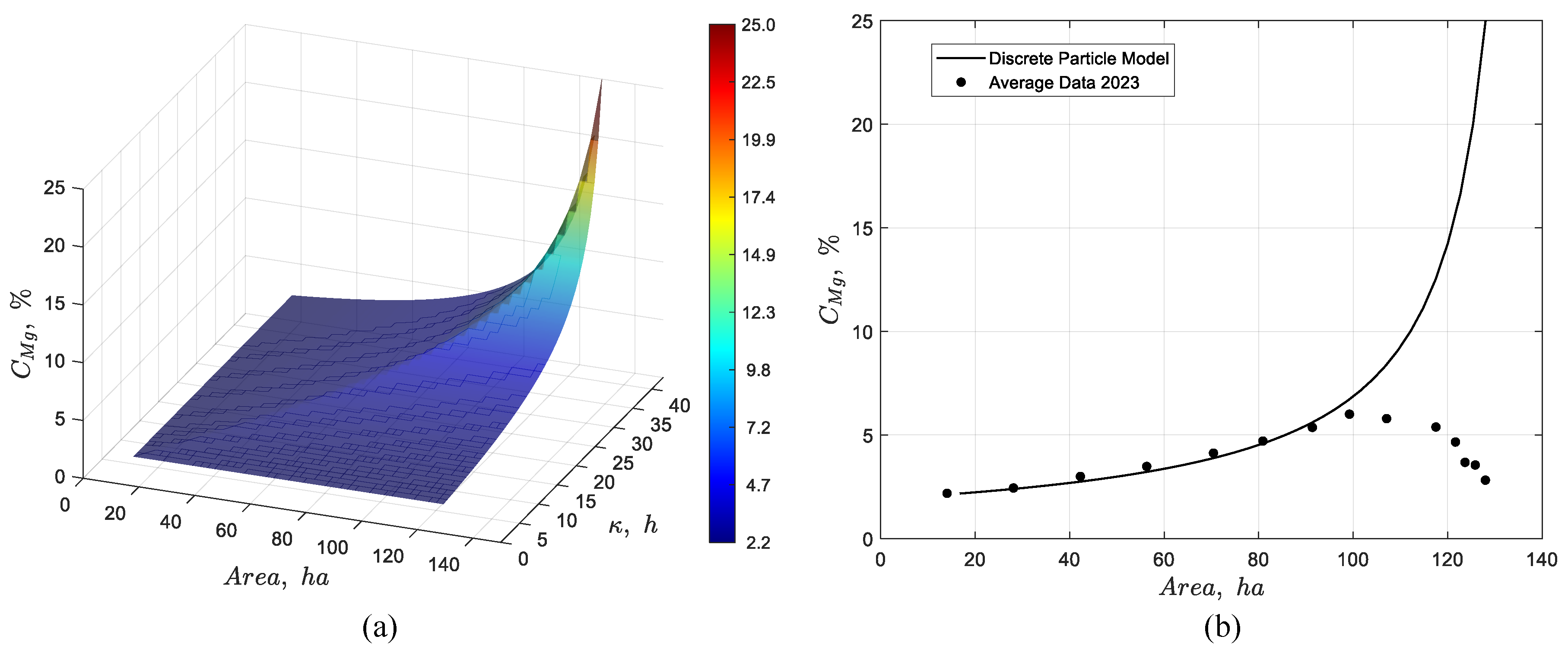
4.3. Model Validation for Magnesium
In the case of magnesium whose inlet concentration was 1.8%, Figure 17(a) illustrates the dynamic simulation using an evaporation rate of 4.2 L/(m2·day), whereas Figure 17(b) presents the model’s steady state response and its comparison with experimental data. In the latter, it can be observed that from approximately hectare 100 onward (around pond 8), the experimental Mg concentration begins to deviate from the predicted values due to the sequential precipitation of potassium carnallite followed by bischofite. Despite the precipitation of these salts, an excellent agreement is observed up to hectare 100.
5. Conclusions
The results confirm that under conditions of zero precipitation of the species of interest the discrete dynamic particle model predicts a steady state concentration profile identical to the profile predicted by the ideal solar evaporation law. However, its capability to indicate deviations arising from solid precipitation highlights its practical relevance. Consequently, the discrete dynamic model is a powerful tool for the optimization of solar evaporation ponds to improve the performance and efficiency of industrial solar evaporation systems.
Author Contributions
Conceptualization, M.S., M.C.R. and R.P.; methodology, M.S.; software, M.S.; validation, M.S., M.C.R. and R.P.; formal analysis, M.S.and R.P.; investigation, M.S.; resources, D.T.; data curation, D.T.; writing—original draft preparation. M.S.; writing—review and editing, M.C.R. and R.P.; visualization, R.P.; supervision, R.P. All authors have read and agreed to the published version of the manuscript.
Funding
This research received no external funding.
Data Availability Statement
The data presented in this study are available on request from the authors.
Acknowledgments
M. Silva acknowledges The National Agency for Research and Development (ANID) of Chile for support through graduate scholarship Doctorado Becas Chile 2016 #21161780.
Conflicts of Interest
Manuel Silva and Diego Toro are employees of Albemarle Ltda. The paper reflects the views of the scientists and not the company.
References
- Silva, M.; Ruiz, M.C.; Toro, D.; Padilla, R. Modeling of an Ideal Solar Evaporation Pond for Lithium Extraction from Brines. Minerals 2025, 15, 1078. [Google Scholar] [CrossRef]
- Kwok, K.S.; Ng, K.M.; Taboada, M.E.; Cisternas, L.A. Thermodynamics of salt lake system: Representation, experiments, and visualization. AIChE J. 2008, 54, 706–727. [Google Scholar] [CrossRef]
- Butts, D. Chemicals from brine. In Kirk-Othmer Encyclopedia of Chemical Technology; Wiley: Hoboken, NJ, USA, 2000. [Google Scholar]
- Bloch, M.R.; Farkas, L.; Spiegler, K.S. Solar evaporation of salt brines. Ind. Eng. Chem. 1951, 43, 1544–1553. [Google Scholar] [CrossRef]
- Cabello, J. Lithium brine production, reserves, resources and exploration in Chile: An updated review. Ore Geol. Rev. 2021, 128, 103883. [Google Scholar] [CrossRef]
- Pueyo, J.J.; Chong, G.; Ayora, C. Lithium saltworks of the Salar de Atacama: A model for MgSO4-free ancient potash deposits. Chem. Geol. 2017, 466, 173–186. [Google Scholar] [CrossRef]
- Hirschmann, J. G. A solar energy pilot plant for northern Chile. Solar Energy 1961, 5(2), 37–43. [Google Scholar] [CrossRef]
- Kee, R.J.; Coltrin, M.E.; Glarborg, P. Chemically Reacting Flow: Theory and Practice; John Wiley & Sons, 2005. [Google Scholar]
Figure 1.
Conceptualization of an ideal solar evaporation pond [1].
Figure 1.
Conceptualization of an ideal solar evaporation pond [1].
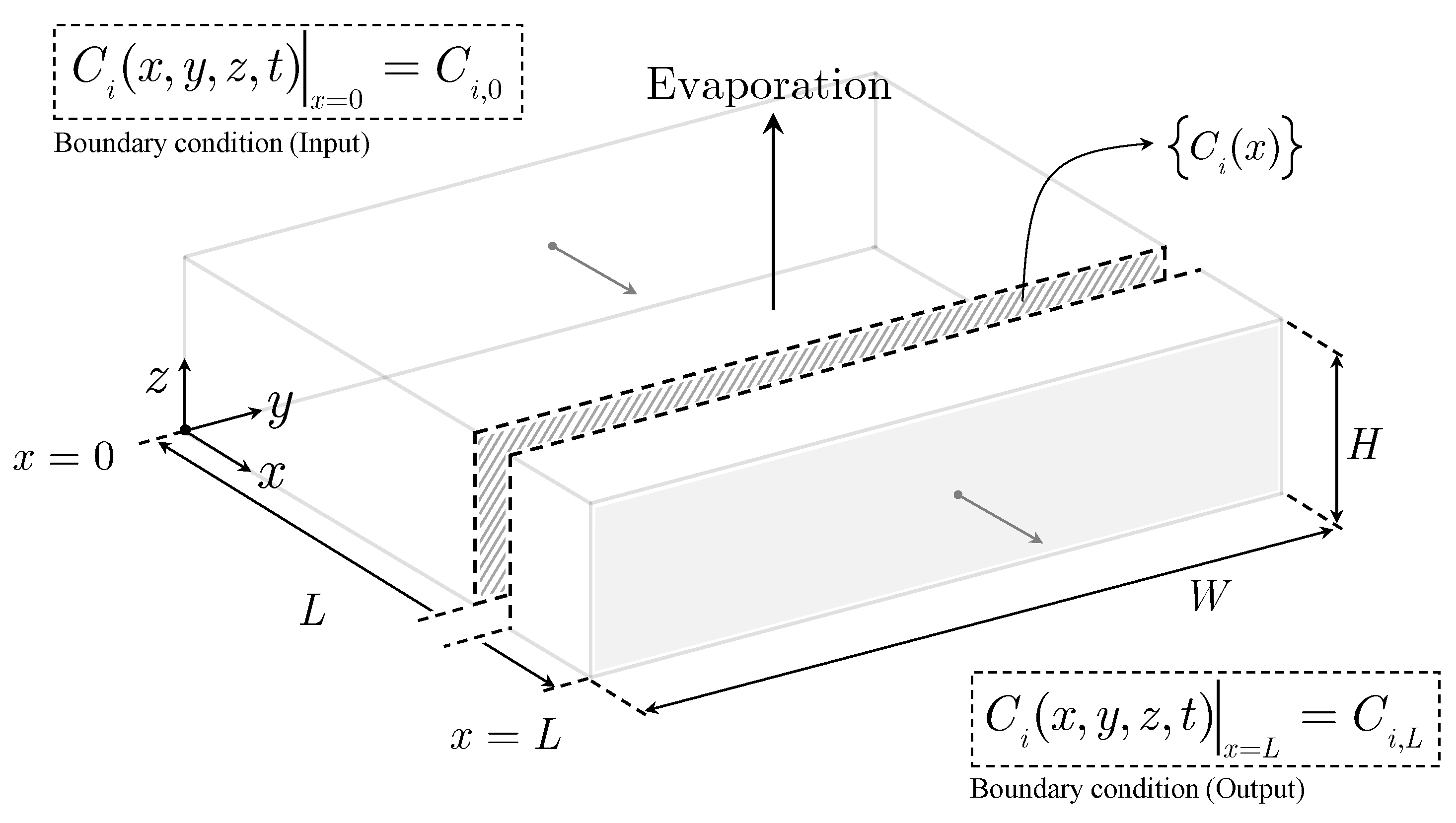
Figure 2.
First iteration of the discrete model for an ideal pond with
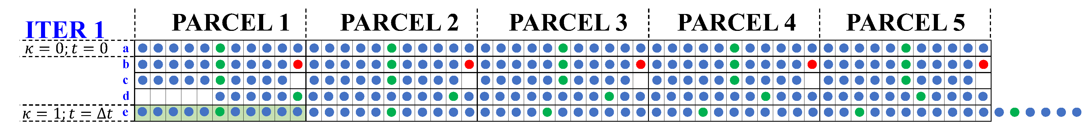
Figure 3.
Discrete particle model simulation until reaching steady state considering 5 parcels.
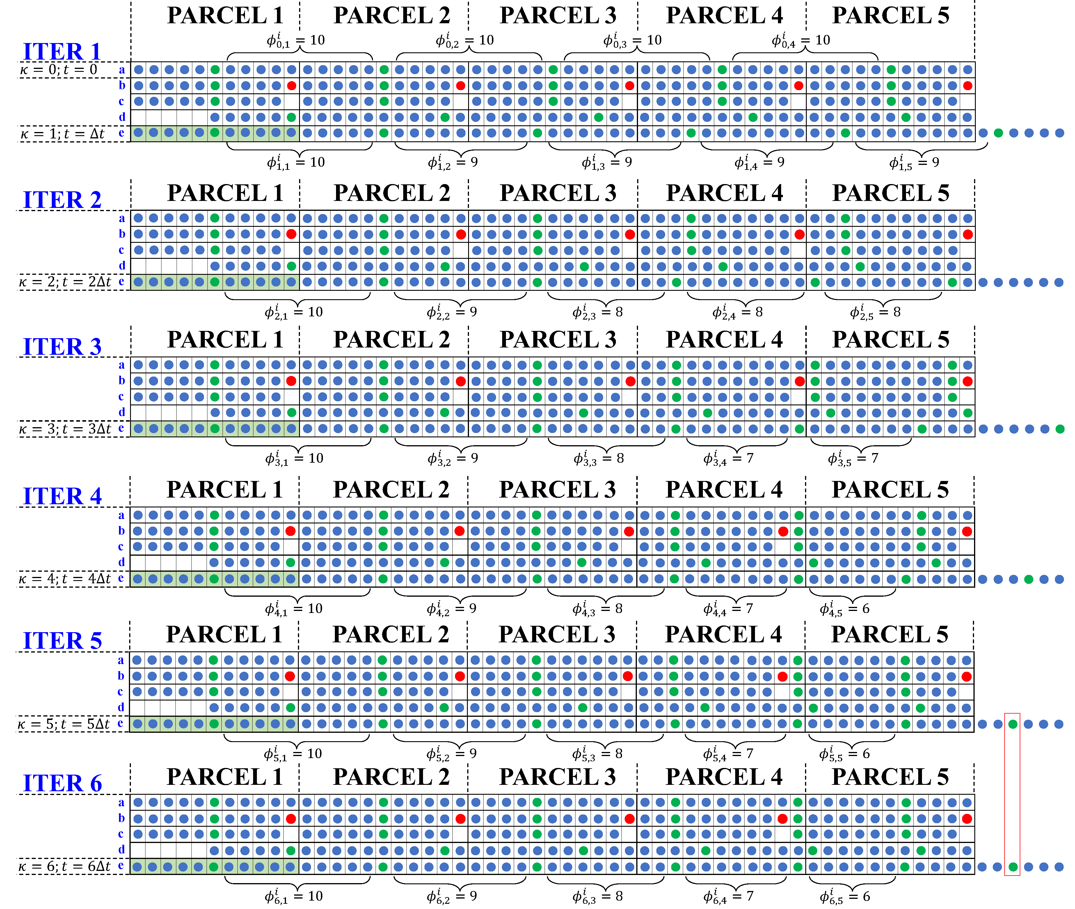
Figure 4.
Dynamic simulation using the discrete particles model for a pond system with a feed lithium concentration of 0.22%, an evaporation rate per unit area of 4.2 L/(m2·day), an average brine flow rate of 66 L/s, and total area of (a) 107 and (b) 131 ha.
Figure 4.
Dynamic simulation using the discrete particles model for a pond system with a feed lithium concentration of 0.22%, an evaporation rate per unit area of 4.2 L/(m2·day), an average brine flow rate of 66 L/s, and total area of (a) 107 and (b) 131 ha.
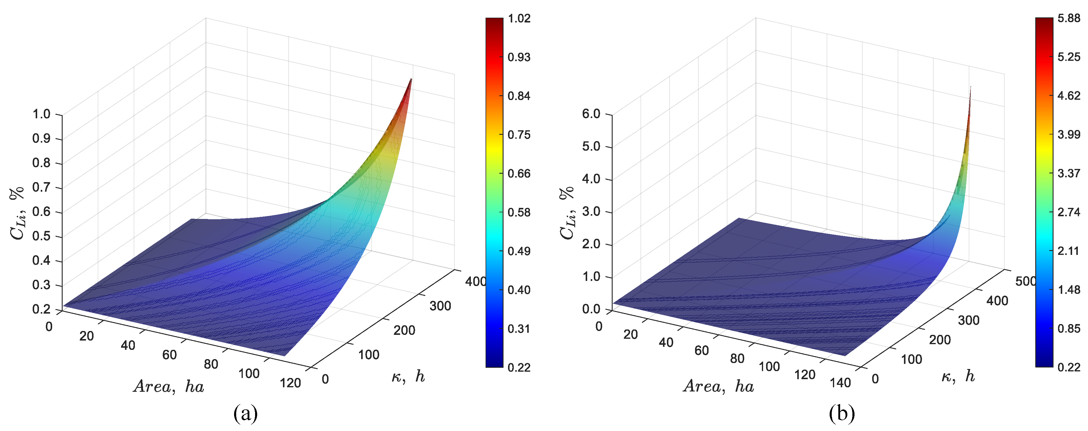
Figure 5.
Comparison between the discrete particle model at steady-state and the ideal solar evaporation law for the pond system with a total area of (a) 107 ha and (b) 131 ha.
Figure 5.
Comparison between the discrete particle model at steady-state and the ideal solar evaporation law for the pond system with a total area of (a) 107 ha and (b) 131 ha.
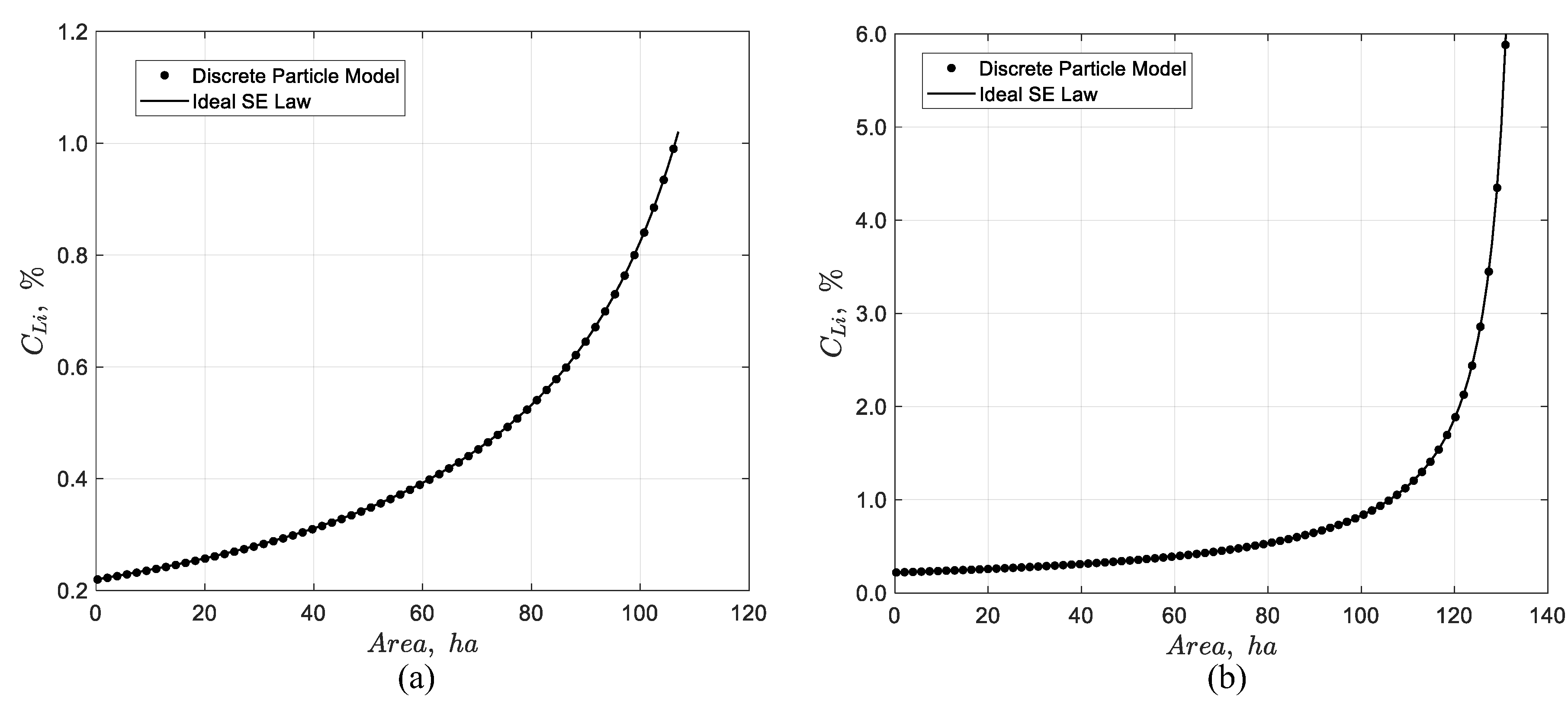
Figure 6.
Dynamic simulation using the discrete particles model for a pond system with a total area of 107 ha, 0.22% Li in the feed, an evaporation rate per unit area of 4.2 L/(m2·day) and a feed flow rate of (a) 56 L/s, and (b) 76 L/s.
Figure 6.
Dynamic simulation using the discrete particles model for a pond system with a total area of 107 ha, 0.22% Li in the feed, an evaporation rate per unit area of 4.2 L/(m2·day) and a feed flow rate of (a) 56 L/s, and (b) 76 L/s.
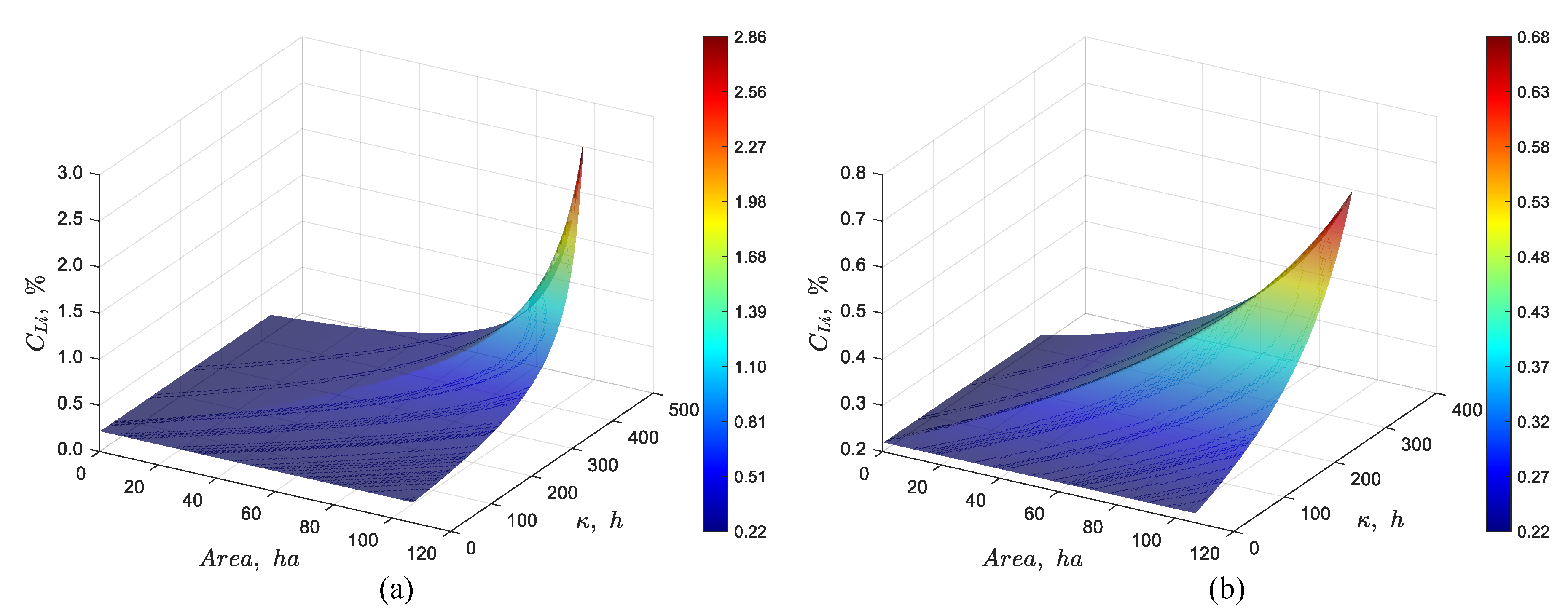
Figure 7.
Dynamic simulation using the discrete particles model for a pond system with a total area of 107 ha, an evaporation rate per unit area of 4.2 L/(m2·day), a feed flow rate of 66 L/s, and a feed Li concentration of (a) 0.20% and (b) 0.24%.
Figure 7.
Dynamic simulation using the discrete particles model for a pond system with a total area of 107 ha, an evaporation rate per unit area of 4.2 L/(m2·day), a feed flow rate of 66 L/s, and a feed Li concentration of (a) 0.20% and (b) 0.24%.
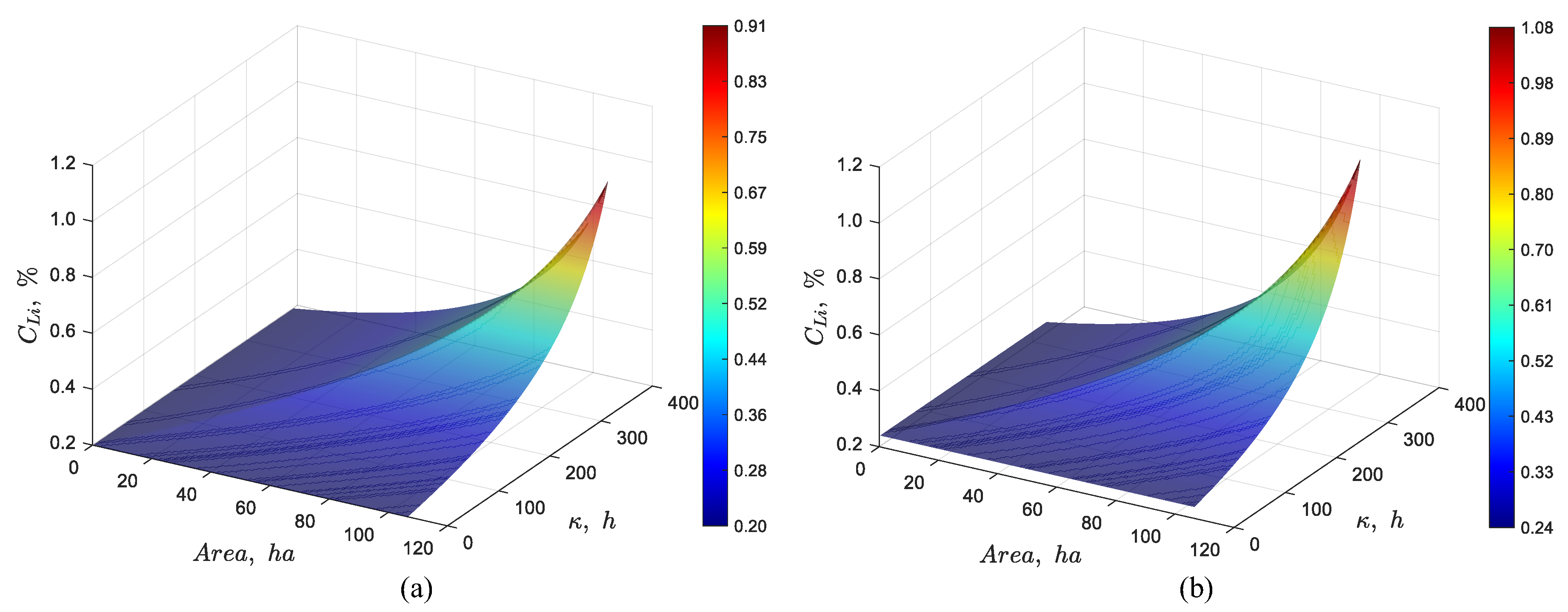
Figure 8.
Dynamic simulation using the discrete particles model for a pond system with a total area of 107 ha, a feed flow rate of 66 L/s, a feed Li concentration of 0.22% Li and an evaporation rate per unit area of (a) 3.5 and (b) 4.9 L/(m2·day).
Figure 8.
Dynamic simulation using the discrete particles model for a pond system with a total area of 107 ha, a feed flow rate of 66 L/s, a feed Li concentration of 0.22% Li and an evaporation rate per unit area of (a) 3.5 and (b) 4.9 L/(m2·day).
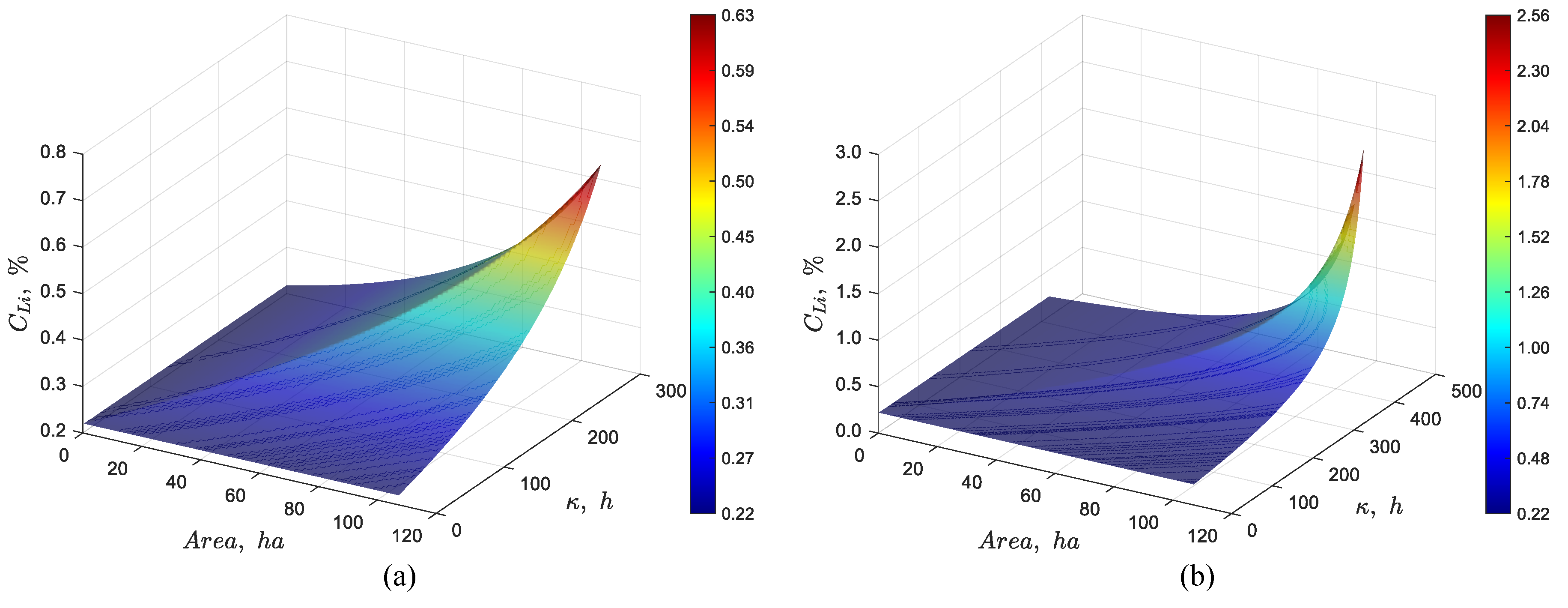
Figure 9.
Smooth and noisy sinusoidal evaporation rates illustrating seasonal variation with and without daily random fluctuations.
Figure 9.
Smooth and noisy sinusoidal evaporation rates illustrating seasonal variation with and without daily random fluctuations.

Figure 10.
Dynamic simulation of the 107-ha pond system considering a feed lithium concentration of 0.22% and an average flow rate of 66 L/s, with (a) a smooth and (b) noisy sinusoidal evaporation rate per unit area.
Figure 10.
Dynamic simulation of the 107-ha pond system considering a feed lithium concentration of 0.22% and an average flow rate of 66 L/s, with (a) a smooth and (b) noisy sinusoidal evaporation rate per unit area.
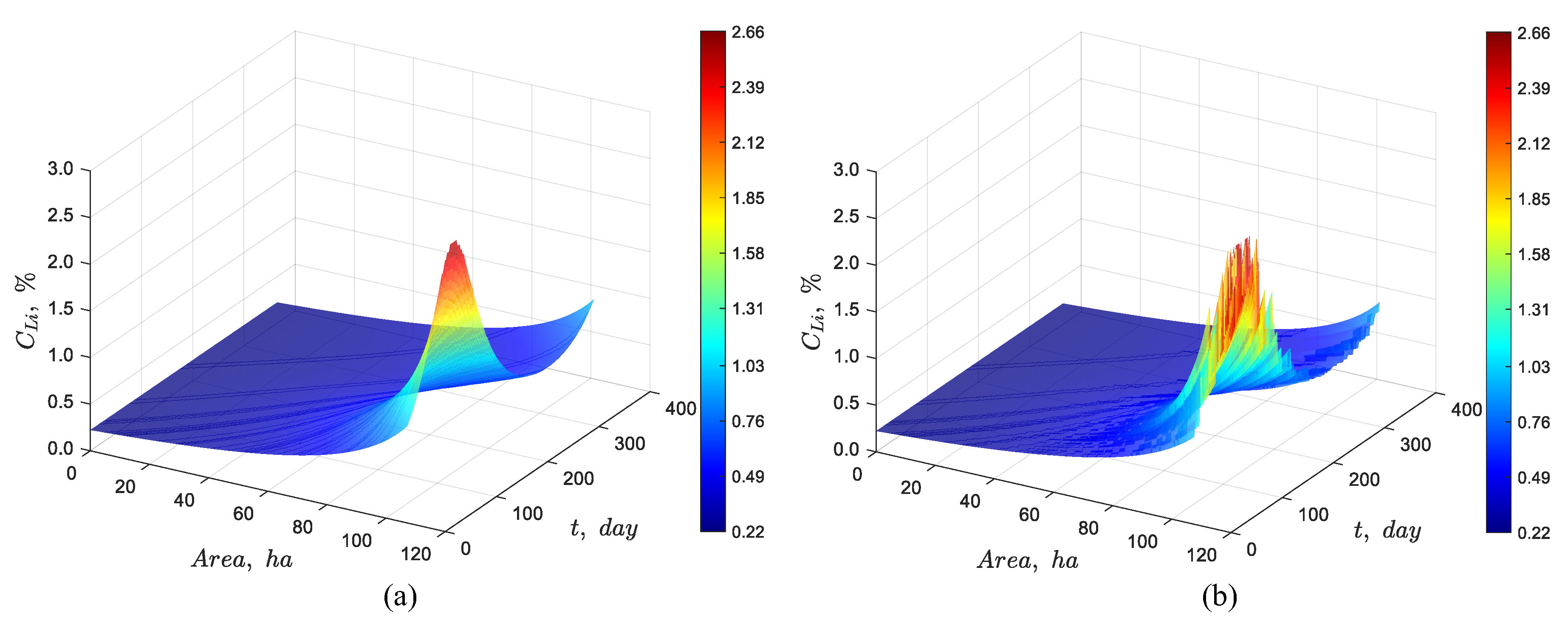
Figure 11.
(a) Optimal feed flow rate found using a stochastic method, and (b) comparison between the measured feed flow rate, its average value, and the optimal feed flow rate found through stochastic optimization.
Figure 11.
(a) Optimal feed flow rate found using a stochastic method, and (b) comparison between the measured feed flow rate, its average value, and the optimal feed flow rate found through stochastic optimization.
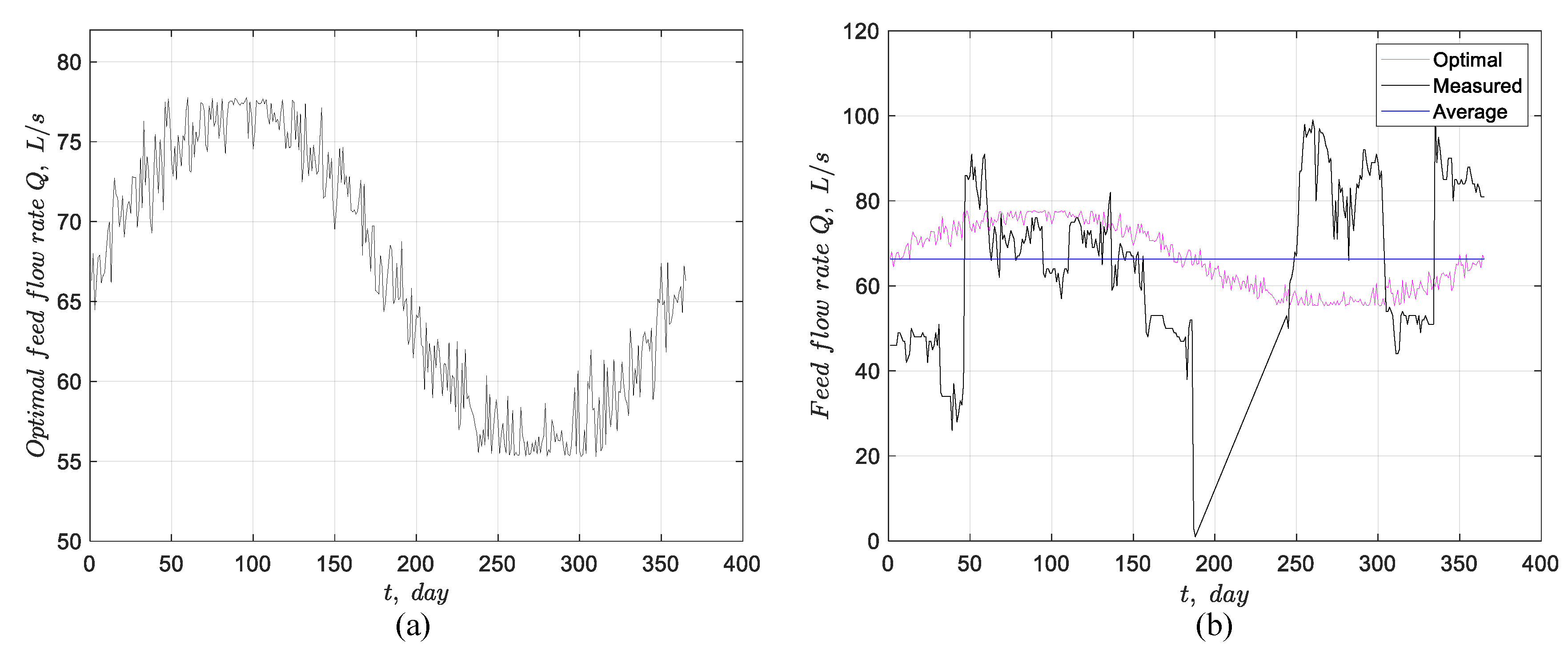
Figure 12.
Stochastic dynamic simulation of discrete particles for a pond system with a feed lithium concentration of 0.22% and a variable evaporation rate, showing that the optimized feed flow rate (a) maintains a constant lithium concentration of ~1.02% over the year for 107 ha, and (b) maintains a constant outlet concentration of ~6% Li for 131 ha.
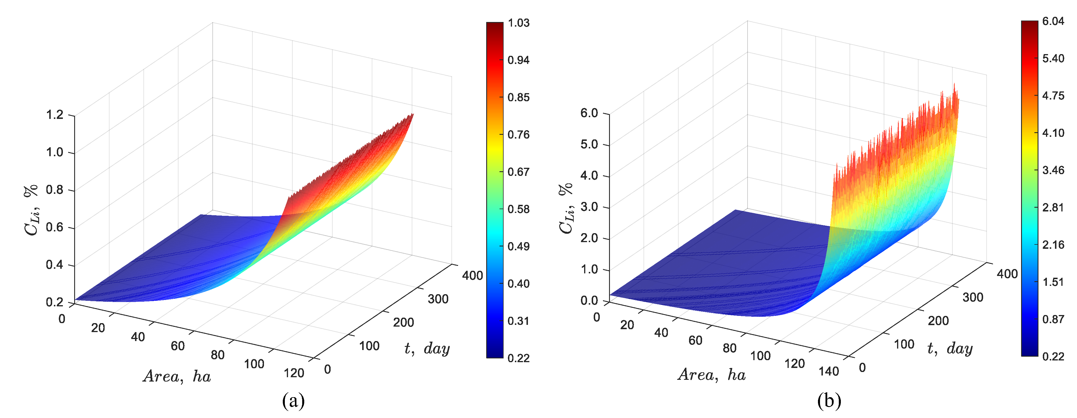
Figure 13.
Dynamic simulation of discrete particles in a 14-hectare pond, illustrating changes in feed concentration and evaporation phenomena at 8 specific times during the simulation considering a feed flow rate of 66 L/s and an evaporation rate per unit area of 4.2 L/(m2·day).
Figure 13.
Dynamic simulation of discrete particles in a 14-hectare pond, illustrating changes in feed concentration and evaporation phenomena at 8 specific times during the simulation considering a feed flow rate of 66 L/s and an evaporation rate per unit area of 4.2 L/(m2·day).
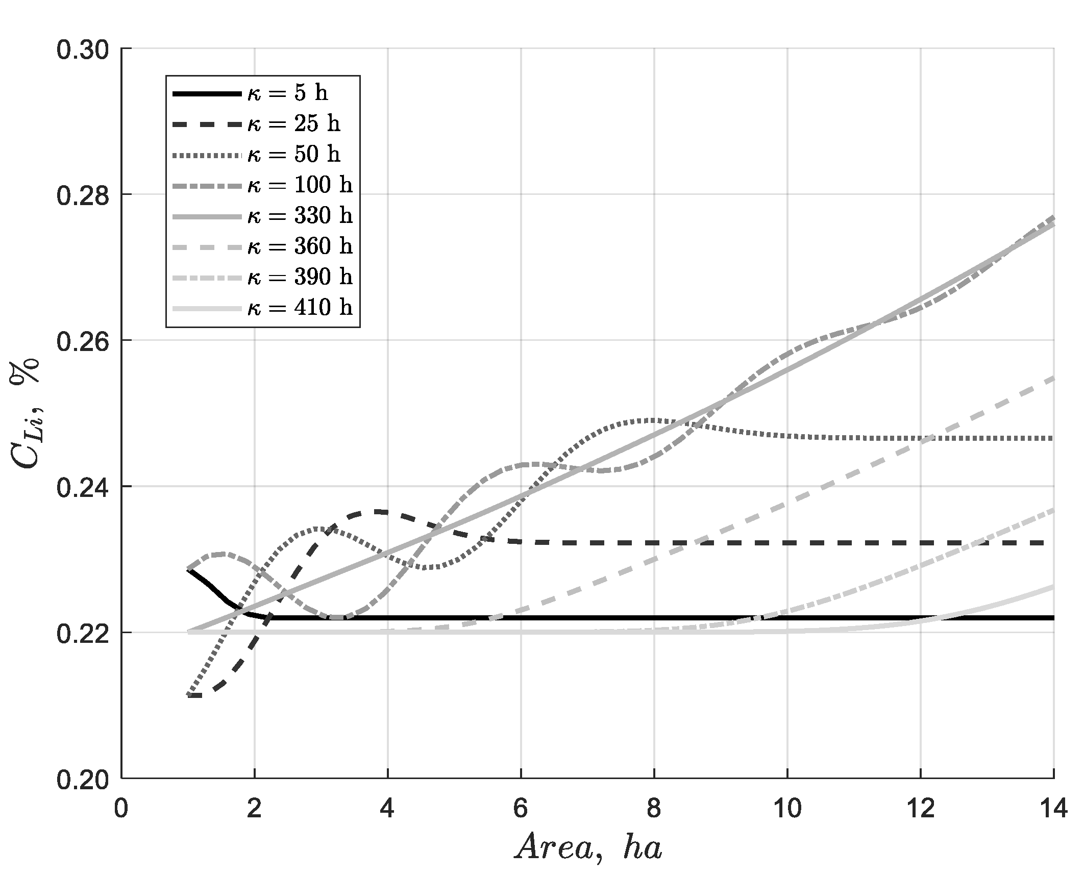
Figure 14.
Dynamic simulation of discrete particles in a 14-hectare pond, illustrating changes in feed concentration and evaporation phenomena over the entire simulation period of 450 hours considering a feed flow rate of 66 L/s and an evaporation rate per unit area of 4.2 L/(m2·day).
Figure 14.
Dynamic simulation of discrete particles in a 14-hectare pond, illustrating changes in feed concentration and evaporation phenomena over the entire simulation period of 450 hours considering a feed flow rate of 66 L/s and an evaporation rate per unit area of 4.2 L/(m2·day).
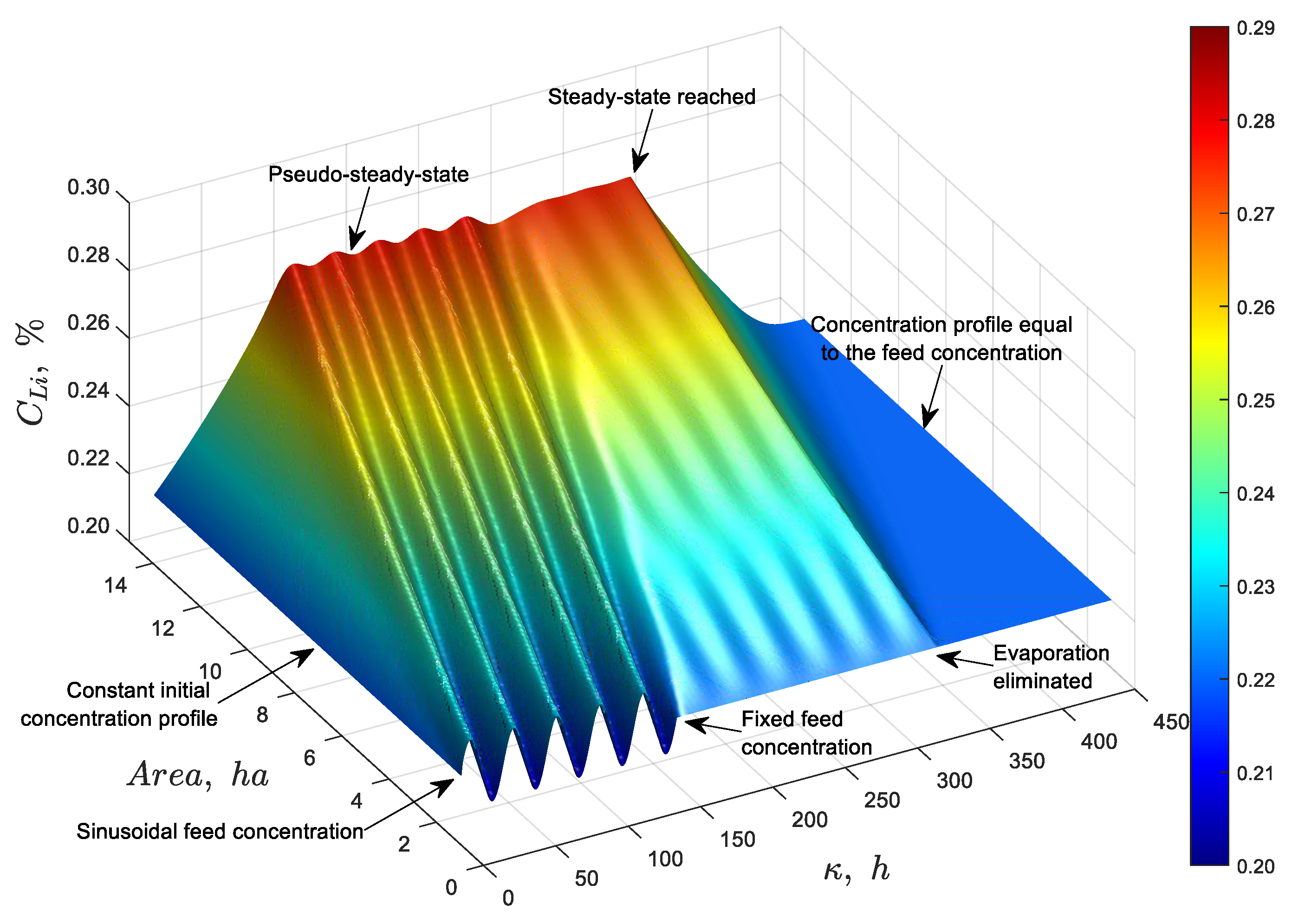
Figure 15.
Dynamic simulation of the discrete particle model for the pond system showing (a) the temporal evolution of the lithium concentration profile, and (b) the steady-state response together with its validation against average experimental data from 2023.
Figure 15.
Dynamic simulation of the discrete particle model for the pond system showing (a) the temporal evolution of the lithium concentration profile, and (b) the steady-state response together with its validation against average experimental data from 2023.
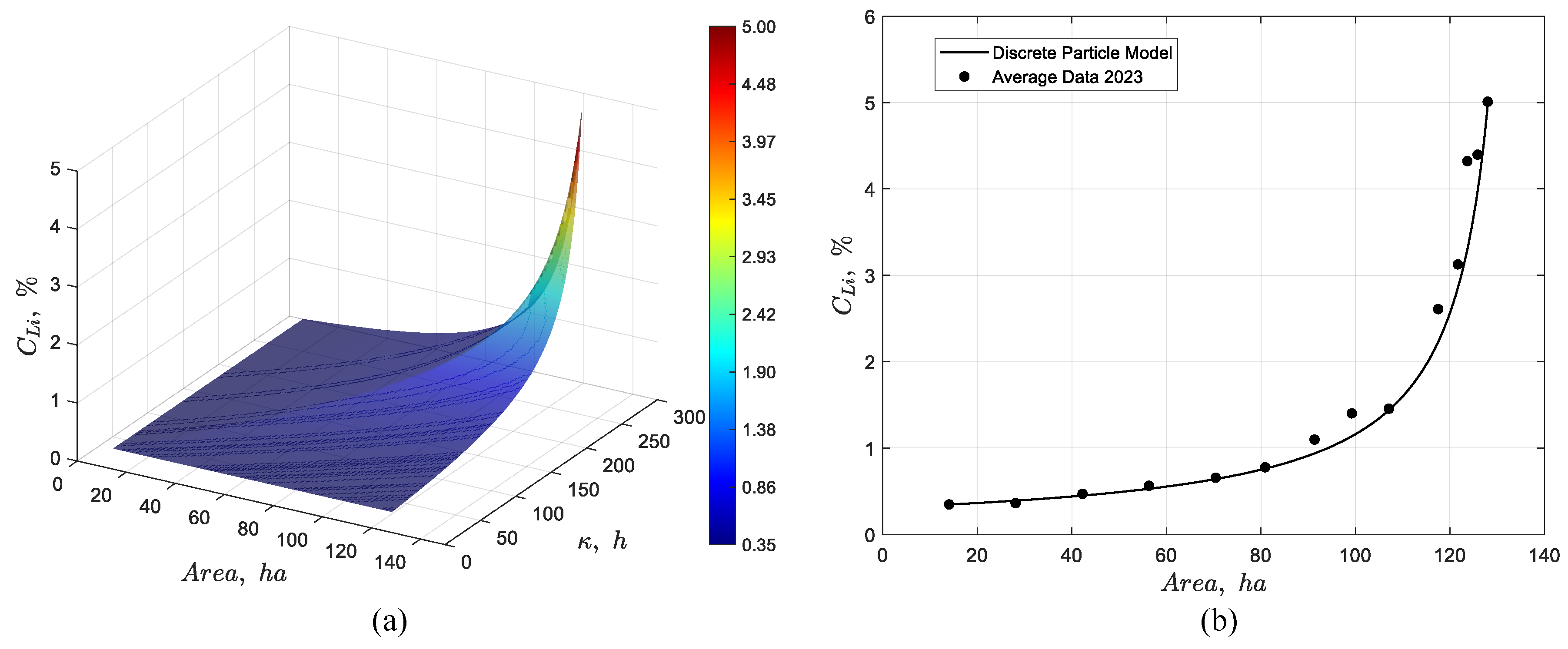
Figure 16.
Dynamic simulation of the discrete particle model for the pond system showing (a) the temporal evolution of the boron concentration profile, and (b) the steady-state response together with its validation against average experimental data from 2023.
Figure 16.
Dynamic simulation of the discrete particle model for the pond system showing (a) the temporal evolution of the boron concentration profile, and (b) the steady-state response together with its validation against average experimental data from 2023.
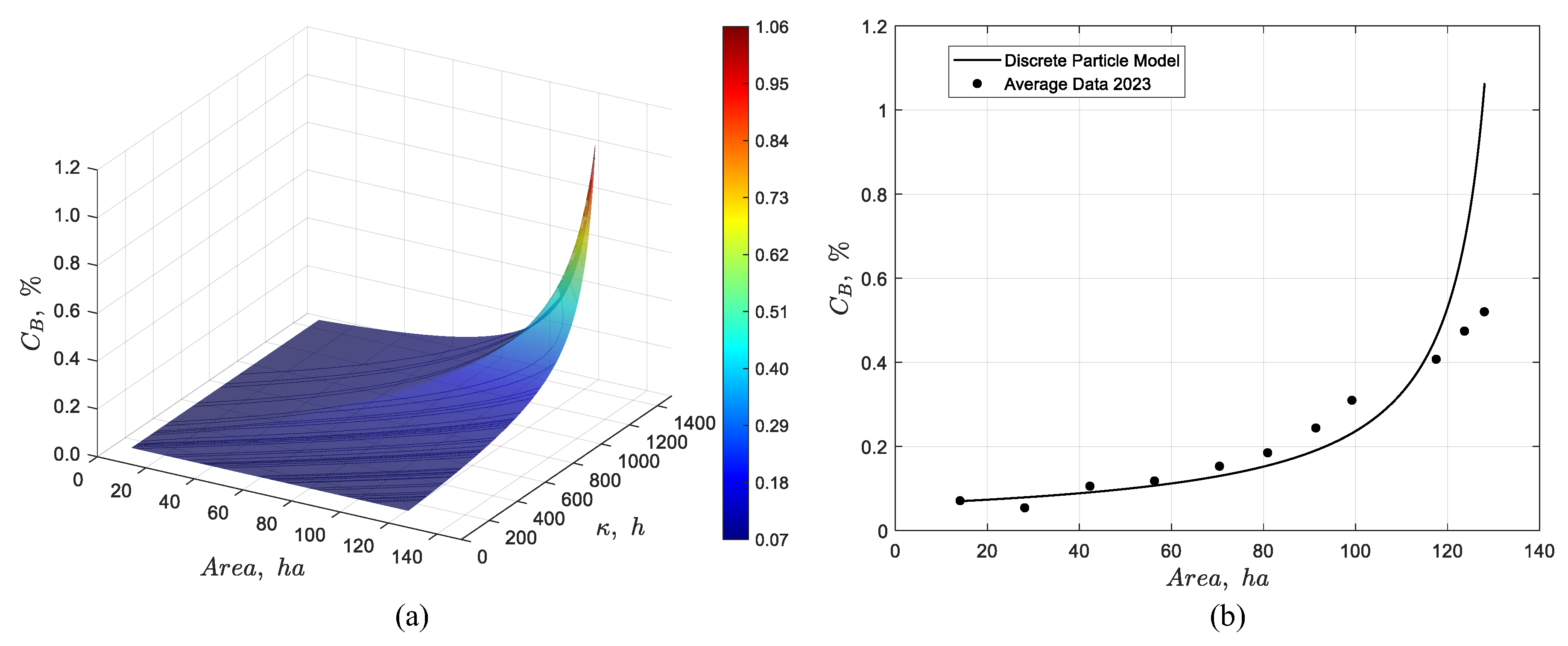
Figure 17.
Dynamic simulation of the discrete particle model for the pond system showing (a) the temporal evolution of the magnesium concentration profile, and (b) the steady-state response together with its validation against average experimental data from 2023.
Figure 17.
Dynamic simulation of the discrete particle model for the pond system showing (a) the temporal evolution of the magnesium concentration profile, and (b) the steady-state response together with its validation against average experimental data from 2023.
Disclaimer/Publisher’s Note: The statements, opinions and data contained in all publications are solely those of the individual author(s) and contributor(s) and not of MDPI and/or the editor(s). MDPI and/or the editor(s) disclaim responsibility for any injury to people or property resulting from any ideas, methods, instructions or products referred to in the content. |
© 2025 by the authors. Licensee MDPI, Basel, Switzerland. This article is an open access article distributed under the terms and conditions of the Creative Commons Attribution (CC BY) license (http://creativecommons.org/licenses/by/4.0/).
Copyright: This open access article is published under a Creative Commons CC BY 4.0 license, which permit the free download, distribution, and reuse, provided that the author and preprint are cited in any reuse.


