Submitted:
04 December 2025
Posted:
05 December 2025
You are already at the latest version
Abstract
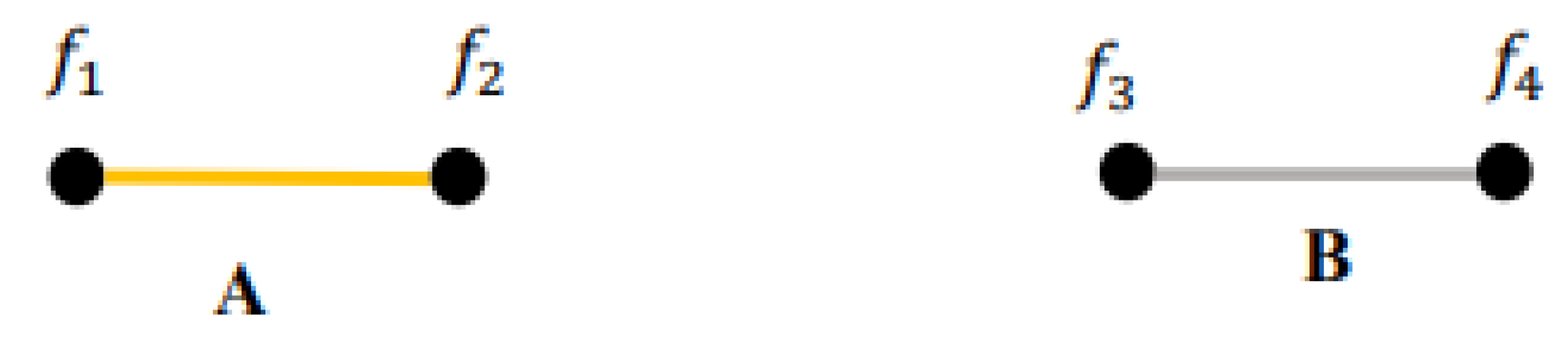
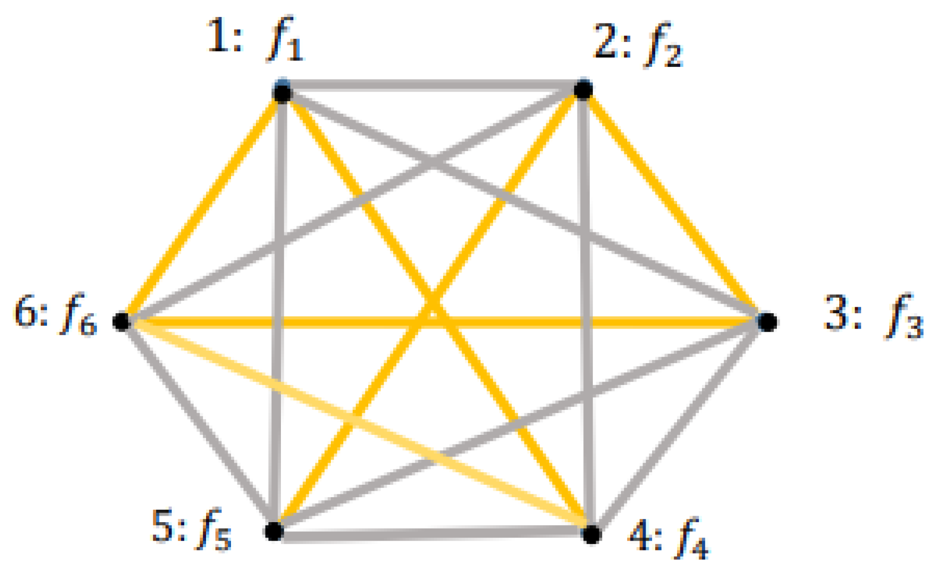
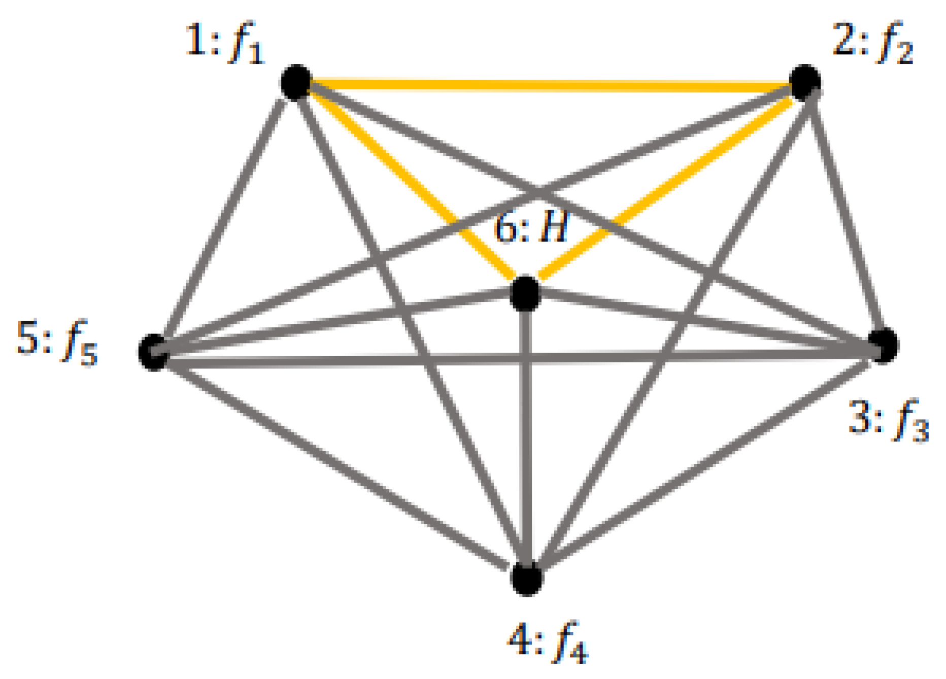
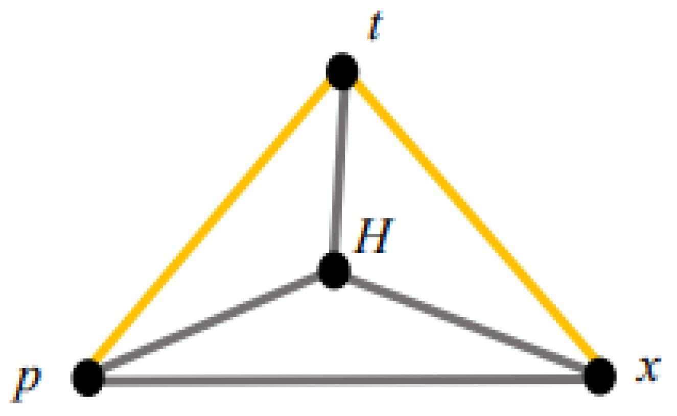
We introduce a new combinatorial framework for classical mechanics - the Ramsey -Hamiltonian approach - which interprets Poisson-bracket relations through the lens of finite and infinite Ramsey theory. Classical Hamiltonian mechanics is built upon the algebraic structure of Poisson brackets, which encode dynamical couplings, symmetries, and conservation laws. We reinterpret this structure as a bi-colored complete graph, whose vertices represent phase-space observables and whose edges are colored gold or silver according to whether the corresponding Poisson bracket vanishes or not. Because Poisson brackets are invariant under canonical transformations (including their centrally extended Galilean form), the induced graph coloring is itself a canonical invariant. Applying Ramsey theory to this graph yields a universal structural result: any six observables necessarily form at least one monochromatic triangle, independent of the Hamiltonian’s specific form. Gold triangles correspond to mutually commuting (Liouville-compatible) observables that generate Abelian symmetry subalgebras, whereas silver triangles correspond to fully interacting triplets of dynamical quantities. When the Hamiltonian is included as a vertex, the resulting Hamilton–Poisson graphs provide a direct graphical interpretation of Noether symmetries, cyclic coordinates, and conserved quantities through star-like subgraphs centered on the Hamiltonian. We further extend the framework to Hamiltonian systems with countably infinite degrees of freedom - such as vibrating strings or field-theoretic systems - where the infinite Ramsey theorem guarantees the existence of infinite monochromatic cliques of observables. Finally, we introduce Shannon-type entropy measures to quantify structural order in Hamilton–Poisson graphs through the distribution of monochromatic polygons. The Ramsey–Hamiltonian approach offers a novel, symmetry-preserving, and fully combinatorial reinterpretation of classical mechanics, revealing universal dynamical patterns that must occur in every Hamiltonian system regardless of its detailed structure.
Keywords:
1. Introduction
2. Hamiltonian Mechanics: Ramsey Interpretation
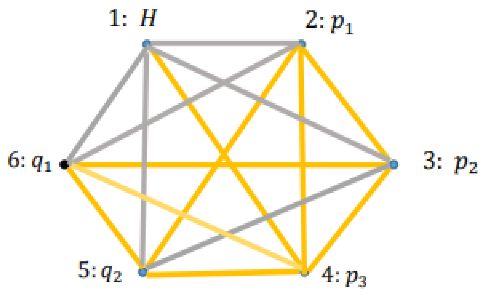
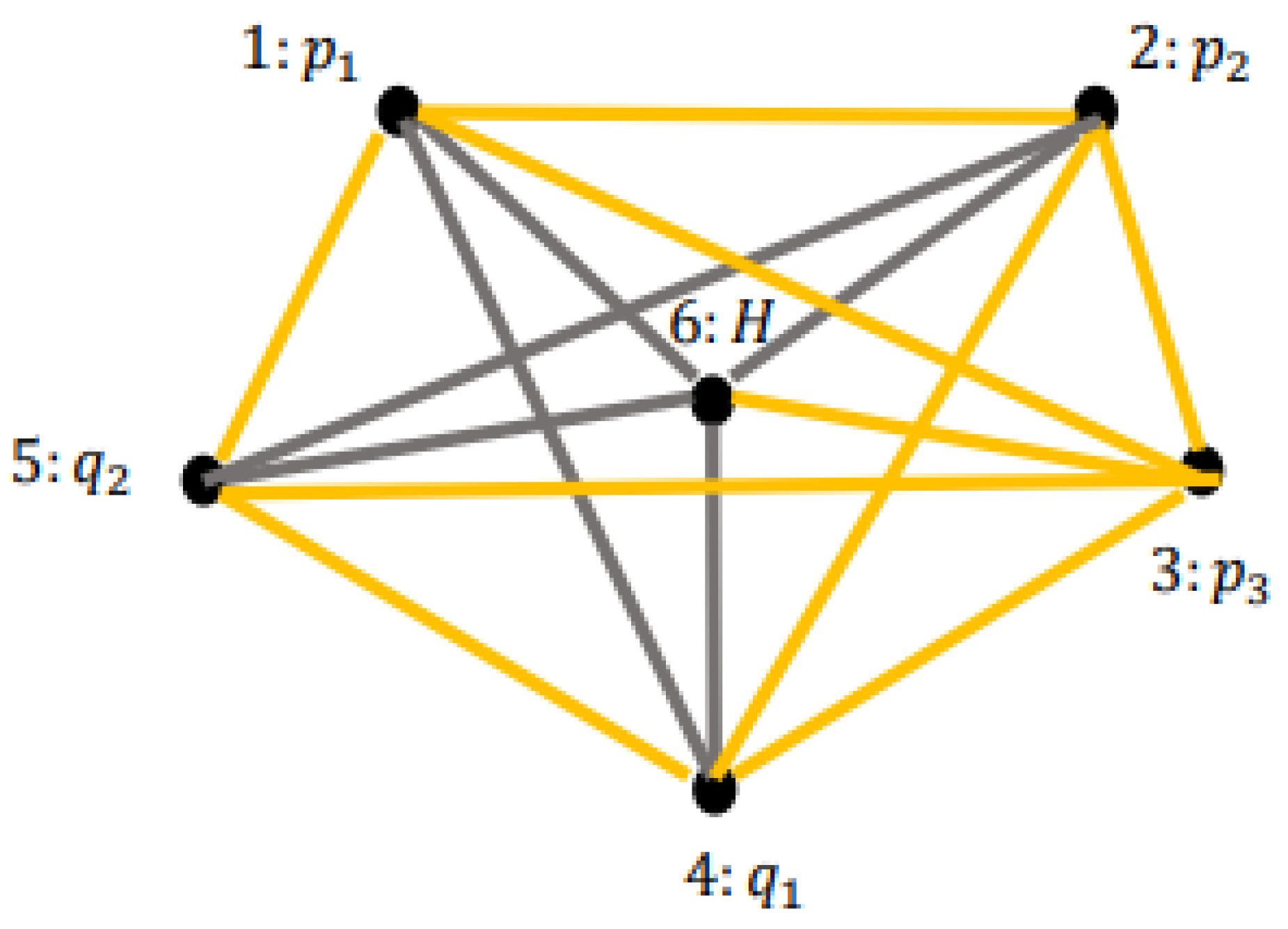
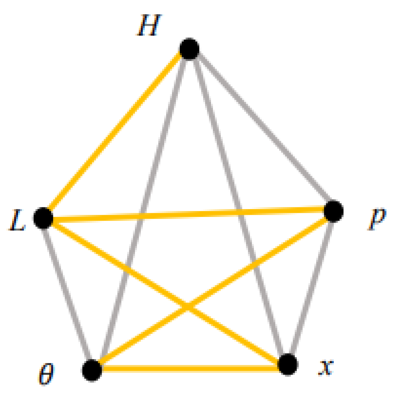
2.1. Bi-Colored Complete Graph Corresponding to the Hamiltonian Systems
2.2. Properties of the Poisson Graphs
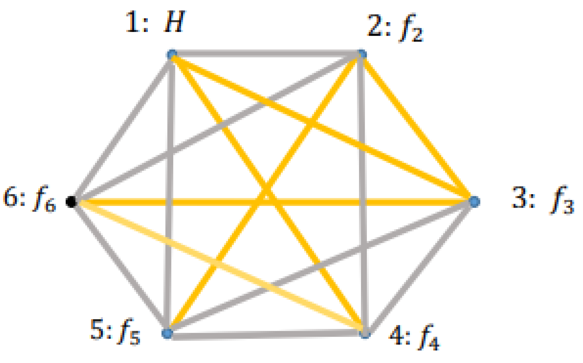
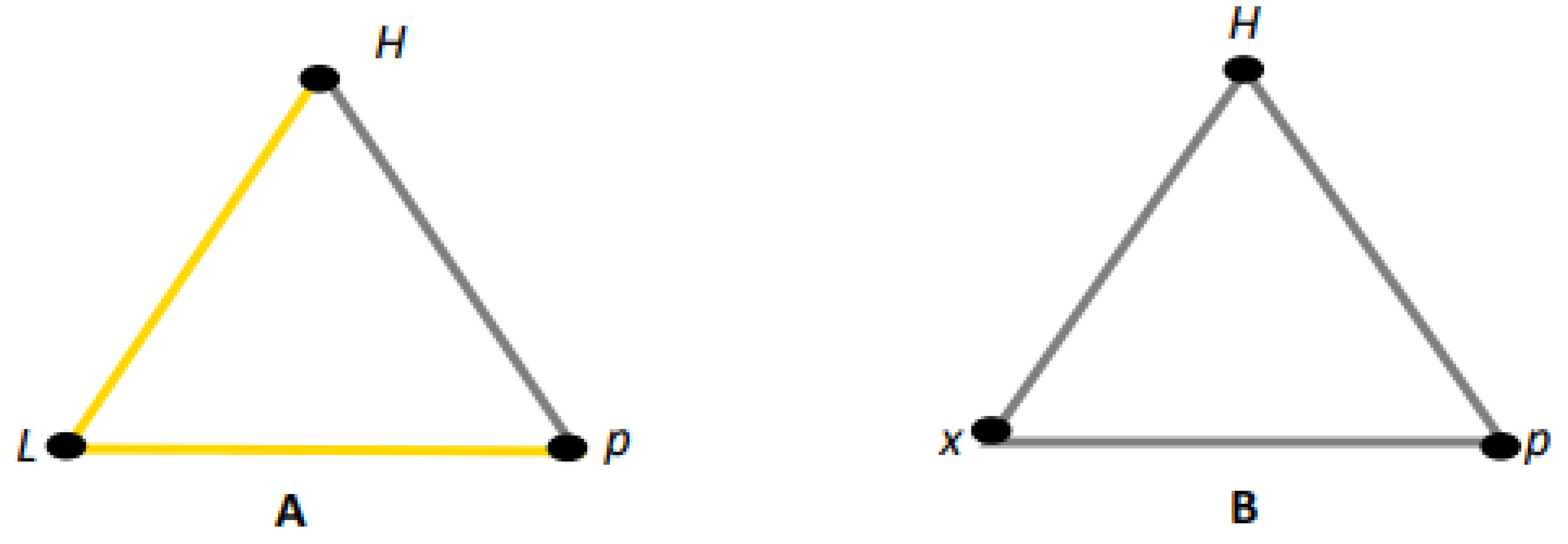
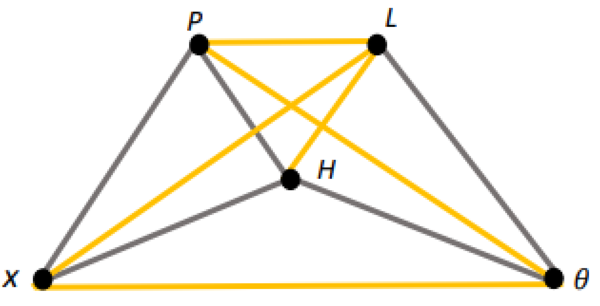
3. Symmetry of the Hamiltonian and the Star Hamilton-Poisson Graphs
3.1. Star Hamilton-Poisson Graphs and the Noether Theorem
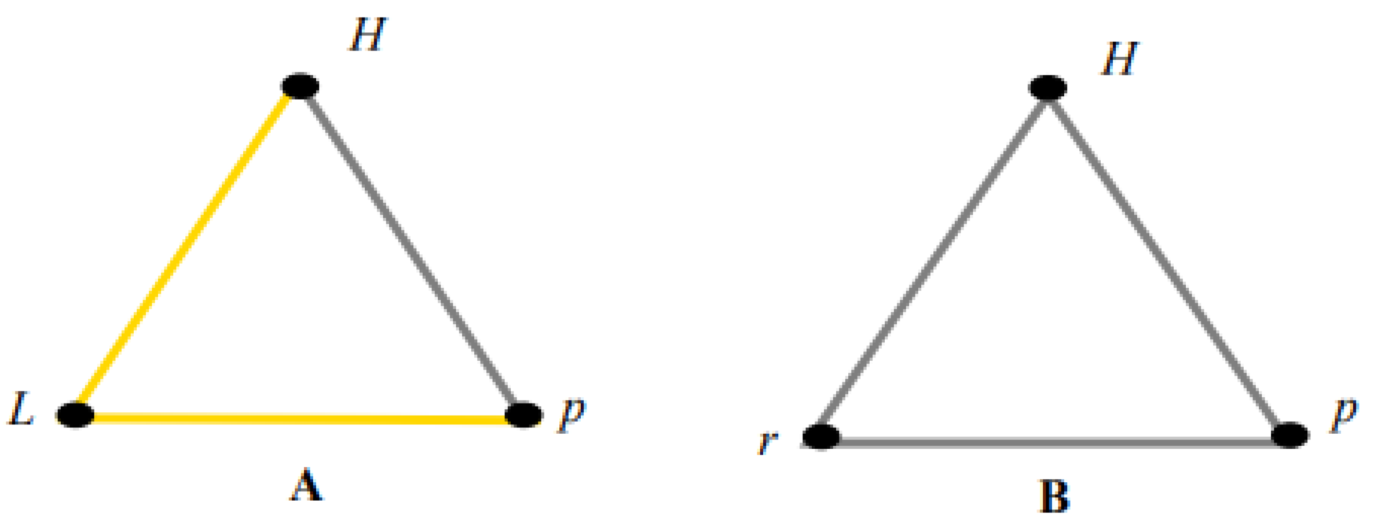
3.2. Cyclic Coordinates Within the Ramsey Approach
4. Analysis of the Systems Possessing the Infinite Degrees of Freedom
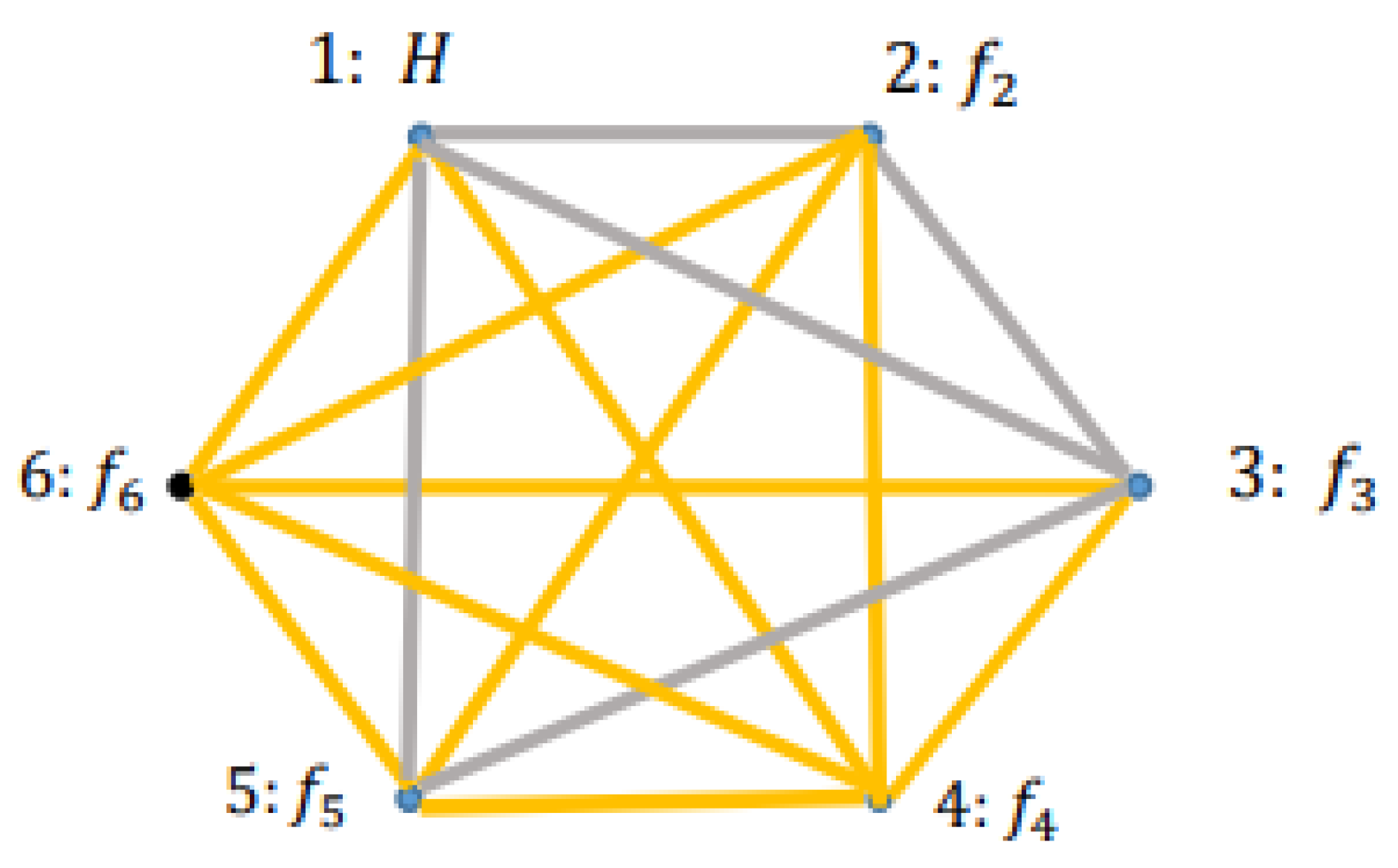
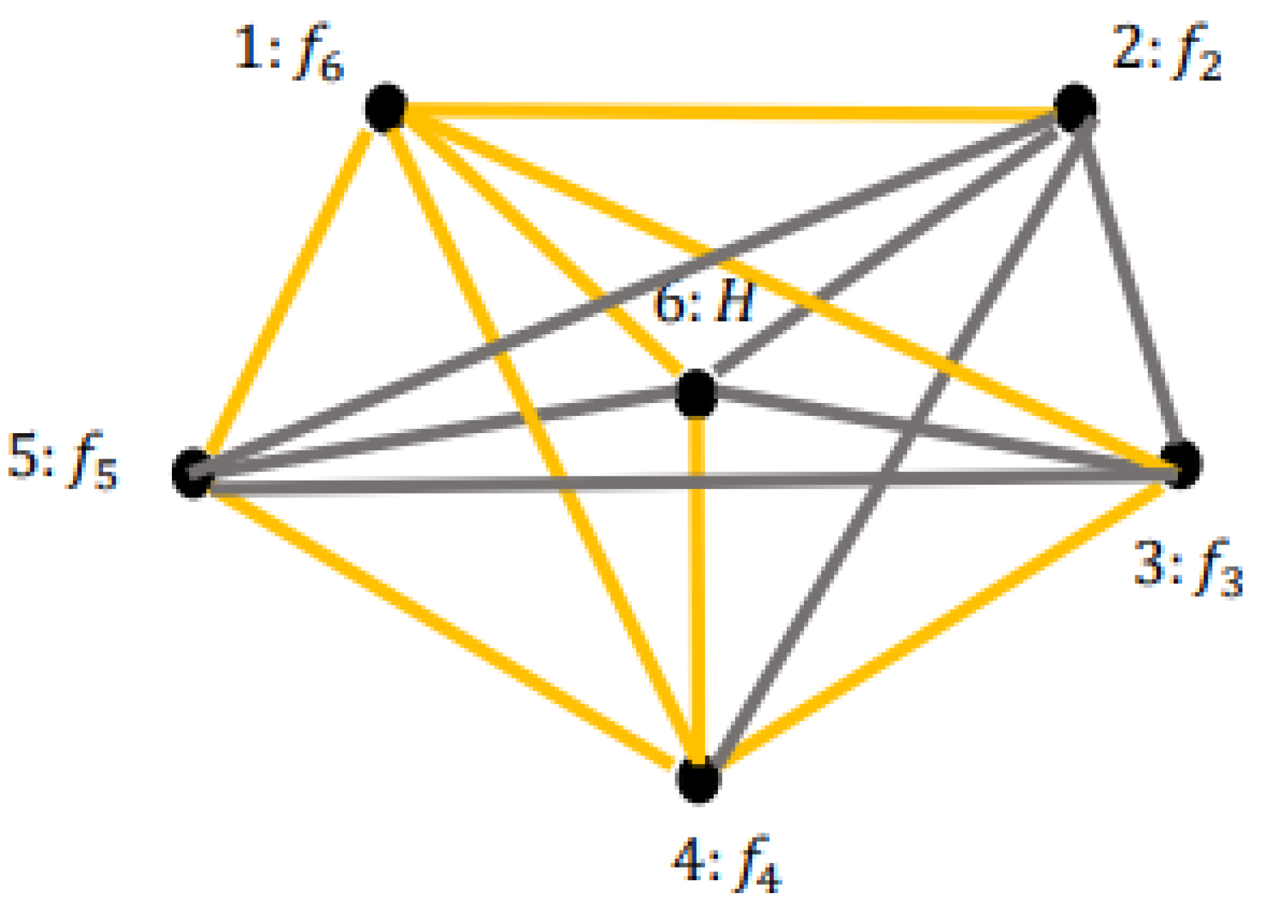
5. Shannon Entropy of the Hamilton-Poisson Graphs

| Color | Triangle | Quadrilaterals | Pentagons | Hexagon |
| Golden | 4 | 5 | 4 | 0 |
| Silver | 2 | 0 | 0 | 0 |
6. Extension for the Hamiltonians Depending Explicitly on Time
7. Discussion
Conclusions
Acknowledgements
Data availability statement
Disclosure statement
Appendix 1
A.1 Analysis of 1D Systems
Appendix 2
A2. Analysis of the Rotation of Rigid Body
Appendix 3
A3. Analysis of the Hamilton-Poisson Graph Obtained for the Two-Dimensional Harmonic Oscillator
Appendix 4
Poisson-Hamilton Graph for the Caldirola–Kanai Hamiltonian Explicitly Depending on Time
References
- Landau LD, Lifshitz EM 1976 Mechanics Vol. 1 (3rd ed.) (Butterworth-Heinemann) Oxford, UK.
- Landau LD, Lifshitz EM 1975 The Classical Theory of Fields Vol. 2 (4th ed.), (Butterworth-Heinemann) Oxford.
- Lanczos C 1970 The Variational Principles of Mechanics (Dover Publications) NY, USA.
- Torres del Castillo GF 2018 An Introduction to Hamiltonian Mechanics Birkhauser, Cham, New York, USA.
- Sardanashvily GA 1995 Generalized Hamiltonian formalism for field theory: constraint systems World Scientific, Singapore.
- Giachetta G, Mangiarotti L, Sardanashvily G 2010, Geometric Formulation of Classical and Quantum Mechanics World scientific, Singapore.
- Azuaje, R.; Escobar-Ruiz, A.M. Canonical and canonoid transformations for Hamiltonian systems on (co)symplectic and (co)contact manifolds. J. Math. Phys. 2023, 64, 033501. [Google Scholar] [CrossRef]
- Ramsey FP 2009, On a Problem of Formal Logic. In Classic Papers in Combinatorics; Gessel, I., Rota, G.C., Eds.; Modern Birkhäuser Classics; Birkhäuser: Boston, MA, USA, pp. 264–286.
- Graham RL, Rothschild BL, Spencer JH 1990 Ramsey Theory, 2nd ed.; Wiley-Interscience Series in Discrete Mathematics and Optimization; John Wiley & Sons, Inc.: New York, NY, USA, pp. 10–110.
- Di Nasso, M; Goldbring, I; Lupini, M. Nonstandard Methods in Combinatorial Number Theory Lecture Notes in Mathematics; Springer: Berlin/Heidelberg, Germany, 2019; Vol. 2239. [Google Scholar]
- Katz, M; Reimann, J. An Introduction to Ramsey Theory: Fast Functions, Infinity, and Metamathematics; Student Mathematical Library (American Mathematical Society) Providence, RI, USA, 2018; Volume 87, pp. 1–34. [Google Scholar]
- Graham, R; Butler, S. 2015 Rudiments of Ramsey Theory, 2nd ed.; American Mathematical Society: Providence, RI, USA; pp. 7–46.
- Li, Y; Lin, Q. Elementary Methods of the Graph Theory Applied Mathematical Sciences; (Springer) Cham, Switzerland; pp. 3–44.
- Chartrand, G; Chatterjee, P; Zhang, P. Ramsey chains in graphs 2023. Electron. J. Math. 6, 1–14. [CrossRef]
- de Gois, C.; Hansenne, K.; Gühne, O. Uncertainty relations from graph theory. Phys. Rev. A 2023, 107, 062211. [Google Scholar] [CrossRef]
- Xu, Z.-P.; Schwonnek, R.; Winter, A. Bounding the Joint Numerical Range of Pauli Strings by Graph Parameters. Quantum 2024, 5, 020318. [Google Scholar] [CrossRef]
- Hansenne K, Qu R, Weinbrenner LT, de Gois C, Wang H, Ming Y, Yang Z, Horodecki P, Gao W, Gühne O Optimal overlapping tomography, arXiv: 2408.05730, 2024.
- Wouters, J.; Giotis, A.; Kang, R.; Schuricht, D.; Fritz, L. Lower bounds for Ramsey numbers as a statistical physics problem. J. Stat. Mech. 2022, 2022, 0332. [Google Scholar] [CrossRef]
- Bormashenko Ed 2025. Variational principles of physics and the infinite Ramsey theory. Phys. Scr. 100, 01504. [CrossRef]
- Bormashenko, E.; Shvalb, N.A. Ramsey-Theory-Based Approach to the Dynamics of Systems of Material Points. Dynamics 2024, 4, 845–854. [Google Scholar] [CrossRef]
- Frenkel, M. Shoval Sh Bormashenko Ed 2023 Fermat Principle, Ramsey Theory and Metamaterials Materials 6 (24) 7571.
- Choudum, SA; Ponnusamy, B. 1999 Ramsey numbers for transitive. Discrete Mathematics 206, 119–129. [CrossRef]
- Soifer A 2009 From Pigeonhole Principle to Ramsey Principle. In: The Mathematical Coloring Book. Springer, New York, NY, pp. 263-265.
- Shannon CE 1948 A Mathematical Theory of Communication. Bell Syst. Tech. J. 27, 379–423.
- Frenkel, N. Shoval Sh 2023 Bormashenko Ed. Shannon Entropy of Ramsey Graphs with up to Six Vertices. Entropy 25(10), 1427.
- Dodonov, VV; Man'ko. Coherent states and the resonance of a quantum damped oscillator. Phys. Rev. A 1979, 20, 550. [Google Scholar] [CrossRef]
- Kottos, T.; Smilansky, U. Quantum Chaos on Graphs. Phys. Rev. Lett. 1997, 79, 4794–4797. [Google Scholar] [CrossRef]
- Landau, LD; Lifshitz, EM. 1991 Quantum mechanics: non-relativistic theory Volume 3 of Course of Theoretical Physics, 3rd Ed., (Pergamon Press) Oxford, UK.
Disclaimer/Publisher’s Note: The statements, opinions and data contained in all publications are solely those of the individual author(s) and contributor(s) and not of MDPI and/or the editor(s). MDPI and/or the editor(s) disclaim responsibility for any injury to people or property resulting from any ideas, methods, instructions or products referred to in the content. |
© 2025 by the authors. Licensee MDPI, Basel, Switzerland. This article is an open access article distributed under the terms and conditions of the Creative Commons Attribution (CC BY) license (http://creativecommons.org/licenses/by/4.0/).


