
Submitted:
04 December 2025
Posted:
05 December 2025
You are already at the latest version
Abstract
Many layer PCBs have many attack surfaces that can hide a Trojan capable of corrupting the processor execution state only with interactions with the processor through external channels such as memory bus. The focus of this research is to monitor the processor execution state only through channels and side-channels that extend beyond the processor chip boundaries. Such a decoupled monitor localizes the program execution state at a blob level - an aggregated form of the program control flow graph. Higher the level of blob aggregation, less demanding are the requirements for the side-channels and execution state revealing channels. Decoupled monitor uses side-channel sensor streams that are naturally created by the program execution (last level cache -LLC- misses). The side-channel sensor streams evaluated in this paper are (1) LLC miss address stream, (2) processor domain power stream, (3) DDR memory domain power stream captured through electromagnetic (EM) emission, and (4) performance monitoring unit (PMU) stream. Blob construction heuristics presents a monitoring overhead trade-off with the localization granularity. A blob is a program level entity whose boundaries are detectable off-processor through side-channel streams. Typical blob sizes we have encountered are 200 instructions as static size and 100s of millions of dynamically executed instructions. The goal of the decoupled monitor is to validate the execution state conformity with a precomputed golden model at a blob and blob path granularity. The monitor is evaluated on a Xilinx Zynq Ultrascale+ ZCU 106 board which contains two ARM processors and a sea of FPGA fabric. Targeted program executes on the Cortex A53 processor for the monitored program state localization. Each of the LLC address, execution path power, performance monitoring unit streams builds machine learning (ML) models for all the paths in a program. The monitor uses these trained ML models to classify the sensor stream data into a Blob/Path. The multiple streams’ classifications are resolved into a single Blob/Path localization based on confidence values of each stream classification. Individual stream’s classification accuracy ranges from 80-90% for the Blob/Path classification. The overall execution state localization is evaluated on a benchmark program "STREAM" with 3 normal execution runs and 2 anomalous runs. The accuracy of this localization is 83.3% for normal runs and 100% for anomalous runs.
Keywords:
dynamic monitoring
; CFI
; control flow integrity
; PCB
; Trojans
; control flow graphs
; performance counters
; power side channel
; EM side channel
; cache coherence
1. Introduction
Over last 25 years, threats of untrusted design flow tools and silicon foundry have emerged. Trusted foundry [1] is a solution to this threat. Trusted design techniques and CAD tools [2] address the design flow end of the problem. A strong underlying assumption is that the printed circuit boards (PCB) are simple enough so that the Trojan chips inserted into them are easily visible, and that they are easily verified. However, modern PCBs have evolved into 32+ routing layers beasts with 6mm+ thick design with plenty of opaque space to hide malicious gadgets. There is relatively little work in techniques to address a PCB-embedded Trojan adversary.
A typical SoC PCB hosts one or more CPU chips, several memory chips, along with additional auxiliary functionality. Any of these subsystems are potential targets of an adversarial attack. In this paper, the integrity of CPU to memory traffic is the main focus. An adversarial Trojan embedded in a PCB can be (a) a listening only adversary leading to data and program IP leakage, or (b) a tampering adversary that modifies the data and/or instructions in-flight with the end-goal of controlling the program behavior to its advantage.
This paper addresses a tampering adversary that modifies program level behavior to its advantage. The main tool and technique to thwart or mitigate these attacks is decoupled or at-distance monitoring. The decoupled monitor detects program execution state integrity (PESI) violations. Control flow integrity (CFI) constitutes a subset of PESI violations. Unlike traditional monitoring techniques [3] and network monitoring techniques such as intrusion detection systems [4], a decoupled monitor is not integrated into the monitored system. It is at some physical distance with lower visibility into the monitored system.
The proposed monitor is decoupled, real-time, multi-modal, and is realized in hardware. The intent is to observe a processor’s execution state visible outside the processor chip boundaries. A PCB embedded malicious agent is able to observe and tamper the processor-memory and processor-peripheral link traffic, which in turn cascades into a tampered program state to the adversary’s advantage. Instead of enumerating the possible domain of program state exploits, we focus on a backbone analysis framework that can support monitoring of a variety of execution state anomalies.
The multi-modal monitor captures the program execution state through multiple side-channel streams - specifically EM, power, last level cache (LLC) miss address, and performance counter streams. A traditional monitor is coupled to the monitored program through computing channels designed to share computing resources. Our decoupled monitor leads to stronger isolation of the monitor. Malware designed to travel through power side-channel or microarchitecture side-channel does not exist at this time leading to long-term/on-going monitor integrity. These lightweight sensor taps into the program state also pose minimal overhead on the program execution environment. This is especially well-suited for real-time programs as well as light-weight computing environments such as an IoT system.
1.1. Challenges
The challenges to building such side-channel sensor streams are multifold. (1) How should the program state be tapped so that the program execution state is not perturbed. (2) When multi-modal sensor streams are used to infer a coherent program state, they need to be carefully and tightly synchronized. This synchronization is extremely challenging. (3) The bandwidth of side-channel sensors streams is small relative to coupled monitors. These challenges are amplified by the fact that the monitoring should have minimal overhead.
The power side-channel capabilities are challenged with a modern COTS processor executing at 4 GHz clock rate with 4-6 wide speculative, out-of-order, superscalar microarchitecture with 100-200 instructions in flight. Reconstruction of the instruction stream at instruction level granularity through power side-channel is not feasible with state of the art [5,6,7,8]. Both the power sample streams and their subsequent analysis are complicated by the required oversampling frequency. Typical power side-channel oversamples at 10x the underlying targeted event frequency, but sometimes this oversampling rate can approach 40x when dealing with countermeasures such as randomized clocks [9]. There are significant engineering hurdles to collecting 160 GSamples/second for each power domain in a modern superscalar processor. The real time analysis of these samples, likely using machine learning or deep learning, is even less practical. Most of the literature in instruction level disassembly is limited to embedded processors with frequency in the range of 20-100 MHz [5,6,7,8].
This leads to the key contribution of this paper in the form of a hierarchical abstraction of the program control-flow graph (CFG) into a blob to overcome the power and EM side-channel shortcomings. A blob typically consists of 2000-10000 instructions. A blob-level control flow graph (BFG) assists our monitor to make this problem tractable. The power and EM side-channel’s role is much coarser, to detect the transitions from one blob to another. This dictates that the blob boundary defining events need to be visible externally closer to the monitor, for example at the memory bus. LLC misses can serve as primary indicators or triggers for blob boundaries. This reduces the power side-channel problem from instruction stream identification to blob stream identification, resulting in a 2000-10000 factor reduction in the problem complexity.
1.2. Contributions
PCB embedded malware detection requires a monitor to be on PCB, loosely decoupled from the processor whose execution state is targeted for tampering by the adversary. The sensor bandwidth from processor execution state to an off-processor-chip monitor is severely limited in comparison to a traditional, tightly integrated, on-processor chip monitor. Our decoupled monitor comprising multi-modal sensor streams includes a novel memory address stream. The main contributions of this work are:
- Low-overhead program tapping for sensor streams without disrupting the program state. Syncing diverse sensor streams to maintain a coherent view of the program state.
- A novel program execution model based on a blob, a coarser control flow graph, enables low overhead multi-modal sensor stream.
- Mapping/transformation of traditional control-flow integrity to parameterized blob-level CFG integrity driven by sensor stream characteristics.
- First prototype of a physical decoupled monitor. Evaluations demonstrate that individual side-channel sensor streams show over 80-90% accuracy in path localization, while the overall monitor accuracy for normal execution flow localization is 83.3%, and anomalous execution flow detection is 100%.
2. Related Work / Background
2.1. Performance Counter Anomaly Detection and CFI
A performance monitoring unit (PMU) or performance counters is a hardware component in a computer system that is responsible for monitoring various performance-related events. Performance counters in a PMU are typically used for program performance enhancement by identifying the sources of program inefficiency such as cache misses. They have been used to flag program execution granularity at a coarse level. CFI may also be monitored through PMU event counters. In this paper, we use PMU counter signatures of various control flow paths from a blob entry to a blob exit to establish a blob path identity. Note that this blob path identification is performed at a distance in a decoupled monitor.
PMU usually contains a limited number of hardware counters that can be programmed to count certain microarchitectural events during the execution of a program. There are six counters on Cortex-A53 processor, the processor in our platform, and we take advantage of all of them to achieve the best blob path detection accuracy.
Besides being used for optimizing the performance of a program, recent studies have shown that PMU can be used for other purposes. Previous research [10] uses PMU counters to recover AES encryption keys by counting cache miss events. The work in [11] has utilized PMU counters to gather the footprint when an embedded system application executing its main event loop. When an anomaly occurs in the main event loop, the abnormal behaviors of a program will affect the PMU counter values, which make the counter values differ from the values collected from profiling the golden model. This leads to anomaly detection. It makes PMU well suited to capture the behavior of a program during run-time. When the control flow of a program execution diverges from its normal execution paths, caused by an anomaly, it modifies the PMU counter value vector over the six counters by an observable quanta. The proposed monitor is able to detect such anomalies with the help of PMU counter vectors. A machine learning classifier can be trained to map a given PMU counter vector into a specific blob path or to an anomalous path.
Karri et al. [12] proposed hardware performance counters for load time and run time program integrity checks. CFIMon [13] monitors control flow integrity through performance counters with branch related events. Both approaches are less general than our approach that uses machine learning derived set of six performance counter events based signature to maximize the blob path identity differentiation.
2.2. Power and EM Side-Channels for Integrity/CFI
Side-channel attacks (SCA) started with cryptanalytic techniques for physical side-channel traces to classify the value of a secret, such as a key embedded into an algorithm, by exploiting the implementation vulnerabilities. The side-channel adversary monitors the hardware execution to record physical attributes such as power [14], timing [15], electromagnetic radiation [16], or even acoustics [17], to extract the secret key used for a cryptographic computation.
One of the first attempts at using power side-channel for instruction level disassembly was Eisenbarth et al. [18] which was limited to disassembling one instruction in a synthetic program for a processor running at about 20 MHz. There have been several instruction level disassembly efforts based on power side-channel in the mean time [5,7,8,19,20]. First three of these differ in machine learning methods and discriminant to push the clock frequency of the processor close to 100 MHz. However, the off-line analysis effort is still not real-time. [7] performs disassembly on a low-end RISCV soft core with low frequency (order of 100 MHz as well). [8] performs instruction level disassembly on on a shared FPGA platform with soft cores again at low frequencies.
There seems to be a dearth of research on using power side-channel to reverse engineer the program control flow graph. [21] uses an embedded microcontroller ChipWhisperer based on STM32F0 microcontroller clocking upto 48 MHz to estimate the control flow of a finite state machine program with two states. Power side-channel traces were used to estimate which of the two states the finite state machine program had entered.
Han et al. [22], on the other hand, develops attacks on a power side-channel based control flow monitor of the kind [21].
There exist several research projects using EM emissions as a side-channel to perform instruction level disassembly [23,24,25,26,27]. They all differ in the machine learning techniques used for signal discrimination and accuracy. [28] proposes an EM based method for profiling a program at a lower cost than the software based profiling. [29] presents a survey of many EM side channel based techniques. Han et al. [30] extends their power side-channel based control flow monitoring of a state machine program to estimate the state through EM side-channel as well.
2.3. CFG Coarsening – Super and Hyper Blocks
Our blob representation is a coarser version of a CFG [31]. A subgraph of the CFG consisting of many basic block nodes is considered a blob.
Since basic blocks tend to be small (5-20 instructions long), for static discovery of parallelism, an aggregated or coarser subgraph of CFG is considered a better candidate. It also tends to reduce the number of branches in such an aggregated CFG.
Hyperblocks [32] and superblocks [33,34] are the main examples of such CFG aggregation. These have traditionally been used for performance enhancement or specialized architectures such as VLIW and predicated execution.
The constraints and criteria for forming a blob are very different from those for forming a hyperblock or superblock.
2.4. Microarchitectural Side-Channels
Microarchitecture level side channels include cache side-channel [35], port contention side-channel [36,37], and performance counters [11]. Cache coherence events have also been used as a side-channel arising out of LLC, which are particularly attractive when the adversary and victim reside on different cores [38].
We use cache coherence events to deconstruct the memory address stream in this research.
3. Motivation or Vision
Problem:
This paper evaluates a monitoring framework when a PCB embedded adversary, such as a hidden chip in an inner PCB layer, compromises the execution state of the processor. The adversary or Trojan has access to only the external links from the processor such as memory and peripheral buses. A tampered memory value, consumed by the processor, eventually leads to control flow corruption. The primary problem addressed in this paper is the monitoring of the processor execution state when the monitor cannot be co-located on the processor. Such at distance monitoring limits the observation channels to only the external links like memory bus coming out of the processor. Side-channels are good candidates to expose the relevant execution state of the processor. This leads to a multi-modal sensor stream available outside the processor boundaries to estimate the processor execution state.
The execution state estimation is challenging even if a model of the program is available to the monitor. In order to verify the CFI of the execution state, minimally, our monitor must be able to infer which control flow edge or node is currently executing within the processor. This is what we call control flow graph localization. This is the minimum requirement for the decoupled, multi-modal monitor.
Solution Framework:
Figure 1 shows the concept overview. The monitor has access to the pre-constructed golden model of the monitored program in the form of its blob level transition graph. The goal of the monitor is to identify Blob/Path identity of the current execution region. Each blob has multiple entry and exit points giving rise to multiple paths. Intuitively, each state in the monitor corresponds to a Blob/Path identity. The incoming multi-modal side-channel sensor streams are analyzed through machine learning classification for a particular Blob/Path identity with a confidence value. The monitor resolves conflicting Blob/Path classifications from different streams through a heuristic that rewards higher confidence values. The PMU stream identifies the blob boundary. This leads to PMU stream check only at blob boundaries. Power/EM stream from blob boundary to blob boundary serves as a reinforcing witness to the PMU stream. They are strong indicators of blob level transition. The LLC miss address stream is somewhat unpredictable. Even though, blob boundaries are formed at LLC miss events, an LLC miss occurs only with certain probability. The address stream also serves as a strong witness for a blob transition (boundary). Power/EM stream is collected at a fixed period throughout the intra-blob computation. We call this window based power/EM stream. These window based power/EM measurements also check the current blob identity periodically based on a sampling window size that keeps sliding forward. The window based periodic sensor streams are also smoothened through hysteresis so that a Blob identity transition is indicated only if it has consistently occurred a few times. The periodic streams are the primary intra-blob path identity verifiers. These are good at detecting attacks that hijack control flow for a brief time period and then bring it back to the original execution path. The blob transition streams (PMU and boundary power/EM signatures) are good at detecting anomalies arising from a control flow hijacking that takes the program across blobs. This paper uses power/EM side-channel to identify a path consisting of 100s of instructions within a blob.
This effort is a preliminary assessment of the feasibility of multi-modal, side-channel streams localizing the program execution at blob path level. This also identifies engineering challenges for such a monitoring system and estimates the practical accuracy and overhead metrics for such a monitor.
The individual side-channel sensor streams show over 80-90% accuracy in path localization. The overall monitor accuracy for normal execution flow localization is 83.3% and for anomalous execution flow detection is 100%.
4. Control Flow Graphs Coarsening Blob Graphs
4.1. Blob Graph
Control flow graphs are a fundamental building block of a compiler [31]. The nodes in a CFG represent basic blocks. Figure 2 shows multiple basic blocks BB0, BB1, ..., BB6. A basic block is a sequence of code with one entry point - at the top. It also has exactly one exit point at the bottom, often with a control instruction like a branch at the end. Basic blocks are important in compilers since they guarantee straight-line control flow from beginning to the end of a basic block, which facilitates code optimization.
For code localization, we need signals visible outside the processor to indicate a program entity. A blob is designed to have an amplified boundary signal. Only the memory accesses that result in a miss in the entire processor cache hierarchy are visible on the memory bus - external to the processor. Hence, LLC miss can be used as a strong indicator in defining a blob boundary. Intuitively, any basic block that has a load/store instruction with a very high LLC miss probability could serve as the boundary basic block within a blob. If the program could be enhanced to have strong external visibility through blobs, load/store instructions from already flushed addresses could be inserted at a boundary basic block to enforce a blob boundary to optimize some other considerations. Figure 2 shows three blobs Blob 0, Blob 1, and Blob 2 that consist of CFG subgraphs.
In the following, we describe heuristics for building blobs.
4.2. Blob Creation
We explore approaches that can be applied solely through static analysis of the program. These may also be augmented with offline profiling of the target program. Figure 3 shows the overall approach of blob creation. An application is compiled to LLVM intermediate representation using LLVM’s C language front-end, Clang ([39], https://clang.llvm.org/). LLVM is then used to emit an ARM v8 64-bit assembly file. Assembly files are generated for both a bare-metal target for execution on the evaluation platform as well as Linux target assembly files to execute on a cycle-accurate computer architecture simulator, Gem5 [40,41]. All local labels are kept as possible entry points of basic blocks in the control flow graph.1 All machine dependent libraries (e.g. startup code, wall time libraries, and console output libraries) are wrapped as black-box functions and omitted from static and dynamic analysis. Generated assembly code is then converted into a control flow graph with nodes representing basic blocks and edges representing all possible paths from a basic block, including back edges seen in loops. At this stage of the analysis, relative symbol offsets are used to map all instructions in a basic block to their eventual virtual addresses given in the initial load address.
Once a complete linked assembly program is created with sufficient symbol annotation to retain the instruction address to CFG mapping, the final executable binary can be constructed. A blob graph representing the coarsened CFG can be created either directly from the CFG using static analysis or from profiling the executable to collect the runtime information. Profiling can be performed either on Gem5 or on the Xilinx Zynq evaluation platform. One advantage of using Gem5 is that many more program execution state metrics are available within the simulation state of Gem5. Many more of these can be used in the future to construct blobs that would otherwise be hard to directly measure in the Xilinx evaluation platform. Additionally, Gem5 provides the ability to run many parallel executions on an HPC platform to generate training data for blob construction when limited number of Xilinx evaluation platforms are available. For these reasons, we use Gem5 to construct our blob graphs. Benchmark binaries are executed on Gem5 running in syscall emulation mode. The Gem5 simulator is configured to mirror the evaluation platform’s processor. There are 2 levels of caches, with the first level consisting of a 32 KB, 4-way set associative data cache and a 32 KB, 2-way set associative instruction cache. The level two cache (last level cache) consists of a 1 MB, 16-way set associative cache with a random replacement policy. The simulator reports all the last level cache misses (LLC misses), which consists of both the address request causing the miss as well as the current value of the program counter at the time of the miss. After complete execution of the program, the total number of cache misses for each basic block is calculated, and this value is inserted into the nodes of the control flow graph data structure. Furthermore, a program counter (PC) trace consisting of an ordered list of all executed instruction addresses is generated for later use in evaluating blobs.
4.2.1. Strongly-Connected Component Approach
Our first approach coarsens the granularity of the control flow graph by grouping strongly-connected components (SCC) [42] of the control flow graph into blobs. SCCs describe a set in a directed control flow graph in which every node is reachable from every other node. By constructing SCCs out of basic blocks (BBs), the normal control flow of a program can be split up into logical sections—loops, setup, and other function calls. We used a standard depth-first search (DFS) implementation of Kosaraju’s algorithm [42] for generating a set of all SCCs in the control-flow graph. Each resulting SCC is labeled as a blob.
While this approach can be performed statically in linear time without profile data, the resulting blobs have two main drawbacks.
- First, some blobs would be overly large. For example, if multiple functions are called in a loop, those functions’ basic blocks and the loop are an SCC—since there is a way for each basic block in the loop to reach each basic block in a function and vice versa.
- Second, isolated basic blocks end up in their own SCC with limited or no externally visible signals. The execution of these blobs is likely to be invisible to a decoupled monitor.
4.2.2. SCC Approach with Dynamic Profiling
To combat issues with overly large blobs and invisible blobs, profiled cache miss data was used. Specifically, we limit the size of blobs using a threshold on number of cache misses. If during creation of a blob this threshold is met, a new blob is created using the remainder of the SCC. Additionally, if blobs are created with no cache misses, meaning they are undetectable, they are merged into other existing detectable blobs. While this method is effective at creating appropriately-sized and externally visible blobs, it often creates blobs that split deeply connected basic blocks (BBs) into different blobs, resulting in rapid transitions between blobs. The blobs splitting based on function calls or other distinguishable markers is a promising future research topic.
4.2.3. Naive Direct DFS Profiling Approach
The initial approach used to delineate blobs was to conduct a depth first traversal of the control flow graph. New blobs are formed every time a basic block with number of misses exceeding a preset threshold is seen. For our initial approach, we empirically chose a threshold value of 50.
The algorithm (see alg:NaiveBlob) is designed to maximize the natural “depth first” flow of software as each basic block executes. As program execution along a control flow graph generally only moves downwards unless a loop introduces a back edge, traversing in a depth first manner ensures maximum spatial locality. Each consecutive basic block is added into the blob until a monitor based on memory access events is able to observe that the program has changed to a new blob.
We assume that a monitor can observe a transition if there is at least 1 cache miss in a new blob. We likely need a higher number of LLC misses to indicate a stronger signal to the monitor establishing a unique pattern of misses. A threshold of 50 LLC misses was chosen after observing that basic blocks with less than 50 instruction cache misses were typically offered a random signature due to random replacement of instruction cache or data cache. Basic blocks with greater than 50 cache misses seemed to exclusively signal high amounts of temporal access. Other benchmarks may yiled different patterns.
| Algorithm 1: Naive DFS Profiling Blob Generation |
|
With a threshold size of 50, 10 blobs were created. Figure 4 depicts a blob-level control flow graph. Most of the blobs connected back to Blob_0. We determined there were two reasons for this: function calls were being treated as a shared node, with an edge inserted from the caller to the function, and another edge from the function back to the caller. This resulted in many functions having many different edges to different call sites.
4.2.4. Natural Loops Approach
The naive approach was undesireable because there were too many blob transitions, many of which lacked cache misses necessary to classify a transition. We determined that one of the primary reasons for this was that the naive approach did not account for the looping behavior present in many programs. Another issue was that each function call was handled by common nodes in the control flow graph, which introduced a significant amount of edge density in the graph. An edge dense graph led to far numerous edges between blobs, leading to too many paths within a blob to efficiently enumerate. This also leads to too many missed blob transitions.
To address these problems with the naive implementation, we created a new algorithm that considered natural loops present in the program. A natural loop is defined as the smallest set of nodes containing the head and tail of back edge, as well as all predecessors of the head of the back edge, though none of the predecessors of the tail of the back edge. A back edge is defined as an edge . A node is said to dominate node if every path from the entry node to must first pass through .
This blob creation algorithm also optimizes function call handling. Each function call is considered a unique instance, and the CFG of the function is inserted at the call site in the caller control flow graph with a unique ID associated with the function call. This “symbolic inlining” allows function call instances to be separated from one another, leading to a far more sparse control flow graph. Such a call site based separation of function calls also more accurately depicts the actual control flow of the graph. The context or preceding conditions prior to a function call differ for each call site, and therefore each call site should be thought of as an independent node.
After symbolically inlining all function calls, natural loops are identified. Many natural loops may overlap, such as in the case of nested loops. A combining or loop coalescing process is then executed in which overlapping loops are combined to remove overlaps. Algorithm 2 shows this heuristic-based approach.
| Algorithm 2: Natural Loop Blob Generation |
|
5. Evaluation Platform & Methodology
5.1. Evaluation Platform
The evaluation is performed on the Xilinx Zynq Ultrascale+ ZCU106 board, a heterogeneous board-level platform built around a modern SoC that integrates a quad core ARM Cortex A53 subsystem, a quad core ARM Cortex R5 subsystem, and an extensive programmable logic fabric [43]. This SoC platform offers realistic architectural settings in which tightly coupled processing elements, a high bandwidth memory hierarchy, and coherent interconnects collectively expose microarchitectural behavior relevant to this study. The board-level layout and system organization are shown in Figure 5.
The selection of this SoC platform is driven by several requirements essential to the objectives of this work. First, the board provides a straightforward mechanism for capturing memory access streams, which is fundamental for evaluating the viability of memory activity as an orthogonal channel for blob-state resolution effectiveness. Second, the platform includes processors of variable complexity, ranging from single-core subsystems to the quad-core ARM Cortex A53 cluster operating across frequency points between approximately 500 MHz and 2 GHz [44]. This diversity allows controlled exploration of execution characteristics under different architectural profiles. Third, the programmable logic fabric offers accelerator-class resources that support the implementation of monitoring components such as blob-transition tracking engines, lightweight machine learning units for power and performance counter analysis, and auxiliary logic for preprocessing and synchronization tasks. Fourth, the board exposes well-documented and easily accessible measurement tap points for multiple power domains, enabling direct board-level observation of processor and external memory power signatures without intrusive instrumentation [43]. This setup enables a decoupled monitor for a processor within a SoC. Although computation occurs on chip, the platform effectively emulates a board-level observation environment because all monitor-state streams are collected outside the processor boundary through interfaces that naturally emerge when SoC components are distributed across a board2.
5.2. Characterization of Power Stream
Circuit level switching activity induced by a specific type of computation and/or data-dependent aspects of computation create a distinct power signature at the pin. Power side-channel taps either a low series resistance to pin or some other point in the power supply network for high frequency sampling. These samples may correlate well with either the secret data or instruction type either in time domain or in frequency domain or in time-frequency domain. Neither of these classical uses of power side-channel are applicable in this decoupled monitor scenario. The secret data extraction requires multiple experiments with the same algorithm execution to be able to extract all the bits of a secret key. This is feasible for a cryptographic encryption/decryption program, since it can be invoked multiple times with the same key. Instruction level identification gives only 1 ns with a 1 GHz single core, single issue processor to detect the instruction opcode, which is quite challenging. Moreover, pipelines spread the instruction level signatures over multiple clock cycles over unpredictable instruction schedules and ordering of events.
In this research, we strive to use power signatures of an execution path to infer if the program execution state is going through a specific path within a blob. For a path of hundreds of instructions, despite the pipeline spreading of the signature, this identification is much more feasible. The time available is hundreds of times larger as well. The path level power signatures also have lower variance due to the law of large numbers.
5.2.1. Power Domains
The Cortex A53 has two distinct power domains that are affected by the instruction execution which is shown in Figure 6. A processor power domain supplies the processor computational cores. A DDR domain supplies the power to the memory. When an instruction executes, it will affect the DDR power domain whenever there is a read or write miss in caches leading to memory activity. This could happen on an I-cache miss during instruction read or during data read/write in a load/store instruction. Every instruction activates various components of the pipeline with variable activation schedules. This activity is reflected in the processor domain. This is the rationale behind capturing a combined processor domain and DDR domain signature of a path through blob.
The processor power domain has additional circuitry on the board to maintain the supply voltage within a small range so that IR drops do not disable the processor. As shown in Figure 6, the processor power domain has capacitance of the order of 900 F along with a power management IC. This large capacitive bank can source sufficient charge to mute the instruction level execution signature peaks and valleys within the constant of the circuit. There is a jumper that can be used to attach the digitizer probe. However signal variation seen at this point with all the 900 F capacitance is not significant enough for path identification.
We removed capacitors from this capacitor bank in 100 F steps to see what effect it might have on the voltage management unit. If more than 400 F of the capacitance is removed, the voltage supply becomes dysfunctional. We do see more of a instruction and data dependent signal variation with 400 F of the removed capacitance. It however still is not as pronounced as it could be with a small shunt resistance across which a probe could be used for a digitizer. We designed and fabricated a small printed circuit board that allows for such a shunt resistance along with all the 10 capacitors of 904 F. It is shown in Figure 7.
The DDR power domain is monitored through electromagnetic side-channel since there was no place on the board to tap it. TBPS01 EM Probe available from Amazon for less than $100 is used to monitor the memory bus activity. The probe from the EM sensor is attached to the same digitizer that samples the processor power domain. We use Signatec PX1500 digitizer. It has a peak sampling rate of 1.5 GHz. It is a good practice to over sample each targeted clock cycle by a factor of 10-20 so that important features are not missed. This gives the highest processor frequency that can be effectively monitored in the range 75-150 MHz. It has 1 GB onboard memory to buffer 8-bit samples. Channe1 1 samples the processor power domain, and Channel 2 records the EM activity corresponding to the DDR domain. The full acquisition setup and representative traces are shown in Figure 8 and Figure 9, respectively.
In Figure 9, synchronized processor-power and DDR-domain EM waveforms are shown, with the Y-axis representing raw ADC values. The processor trace exhibits a brief disturbance near 3 s, indicating the stall caused by an LDR-induced LLC miss. The DDR EM trace shows a temporally aligned burst of high-amplitude activity corresponding to the resulting off-chip memory fetch. The close alignment of these ADC-level signatures highlights the coupling between the cache-miss event and DDR activation, captured using the Signatec PX1500 digitizer.
5.3. LLC Miss Address Stream
Since Zynq ZCU106 is an SoC platform, it allows for new behavior/core to be created in the FPGA fabric of LUTs. This core can also have coherent access to the memory with a shared view with the other cores of the Cortex A53. Towards this end, Xilinx provides an interface with cache coherence fabric through cache coherence interface (CCI) for the LUT based memory client. Figure 10 shows this CCI interface. When an LLC miss occurs from one of the cores of Cortex A53, it shows up at the cache coherence common bus connecting all the memory clients. This address (and data) is broadcast to all the clients through CCI. This allows for the LUT based memory client to garner the address (and data) from the CCI interface giving us an easy access to the memory address stream.
Figure 11 shows an example address trace from the Stream benchmark with the overlaid ground truth blobs. We can see that each blob appears to have a unique pattern for the sequence of addresses. This is true across multiple executions of the same blob (e.g., blob 4) even for different entry points to the blob (e.g., blob 30 and 31). However, sometimes a different path through the blob may produce a very different address trace (e.g., blob 32 vs blob 30 and 31).
In order to produce tokens that continually localize the program execution at blob/path level, last level cache misses addresses are recorded through the CCI. A token is a label that uniquely identifies a blob/path derived through machine learning on the raw data. Additional type flag indicating the memory operation type (read, write, and maintenance operations) is also kept. The input cache stream is first analyzed for outliers. Outliers are defined by any data point that has a modified Z-score greater than 2. Outlier filtering removes many stray miss values that seemed to decrease the accuracy of classification into a blob and blob path.
After removing outliers, the cache miss data is windowed into 100 sequentially adjacent cache misses. A value of 100 was selected experimentally to optimize the tradeoff between prediction latency and prediction accuracy. Each set of 100 sequential cache misses are then mapped to a 50 dimensional bin vector. A series of 50 symmetric bins are distributed across the address range of the data for both memory read and write accesses. The range is determined by the minimum and maximum outlier cutoff values, calculated by . Bin vectors are filled by counting the number of cache misses in each bin range across the 100 cache miss wide window. Finally, all other remaining cache misses in the window are summed in a final bin of the vector.
All feature vectors are generated over non-overlapping windows of the cache channel. The vectors are then used to train a random forest model consisting of 5 decision trees. This model was chosen as it provides a probabilistic prediction with low prediction and training latency.
5.3.1. Explicit State Triggers
Although blob creation and identification based on externally-visible signals that an application implicitly generates is desirable because it does not require application modification, it lacks the ability to control for disambiguation of paths within or across blobs. It also does not have a control knob for modulating the latency of anomaly detection. As a fall-back, explicit state triggers can be inserted into the application executable. These explicit state triggers directly cause an externally-visible signal to be generated at a particular point within the blob graph. We insert these signals directly into the application assembly by redirecting known BB target symbols. We use two main types of explicit triggers – (1) causing an artificial cache miss of a known, already used address via a cache flush instruction and (2) writing to a known and predetermined, but reserved address.
In order to leverage a cache flush instruction (e.g., CIVAC in ARM), we must identify a particular address that we reliably expect to be accessed by the application at the time of the trigger. Therefore, we select an instruction to flush since fetching of instructions is strongly dependent on the location within the CFG (and thus blob graph). While data accesses can be correlated to locations within a blob graph they are more likely to be aliased across different points since the same data locations are often accessed in multiple locations within a program. As a prototype, we flush the instruction immediately after a function call (i.e., the return address of a function). We instrument the call to flush the cache block pointed to by the return address. Then, when the matching return instruction is executed, the flushed cache block is fetched resulting in the externally-visible signal. Such an approach is relatively low-overhead per trigger (roughly two added instructions and an additional cache miss) and does not require any reserved memory location.
A more flexible approach selects a reserved address. The reserved address is intentionally flushed from the cache when the application is loaded. At each trigger point in the blob graph the reserved address is written to and then flushed. This is advantageous in that additional information can be externally signalled. This is the approach we use to generate the performance counter stream (see sec:pmu-stream).
5.4. Performance Counter Stream
All modern processors support a performance measurement unit (PMU). This unit consists of programmable counters. Some set of microarchitecture level events that affect performance can be counted during a program execution. These events can include L1 instruction cache #misses, #retired instructions, #issued instructions, clock cycles count, and #branch mispredictions. They are a separate hardware unit enabling continuous overhead-free monitoring without posing an overhead on the application execution. A small number of performance counter registers are supported. For instance, ARM Cortex A53 supports 6 physical counters. Each counter register can be bound to a specific event through programmable registers. For instance, counter 0 could be associated with #L1 D-cache misses.
ARM provides low level instructions to manage the PMU interface. For instance, ARM_PMU_Enable and ARM_PMU_Disable enable and disable the PMU. Similarly, ARM_PMU_Get_CCNTR reads a performance counter. PMU counter values are read at each blob boundary and then these values are written to a specific memory address that is predefined by the CCI. When the target application is running on the platform, the CCI will constantly monitor the predefined memory address. All memory writes to that memory address will be captured by the CCI and the CCI will generate a set of markers which includes the corresponding PMU counter values. This set of markers will be put into the address stream and then later consumed by the monitor.
We use all of the six programmable PMU event counters and the non-programmable PMU cycle counter to capture the CPU activities during the execution time. The six programmable PMU events we picked are: #instruction retired, #L1D cache access, #L1I cache access, #predictable branch speculatively executed, #Load retired, and #bus cycles. We construct our PMU counter vector by using these seven counters. By doing so, the characteristics of an execution path in all of the blobs can be abstracted by a PMU counter vector.
The machine learning training data are collected by running the golden model program multiple times. In the training data, each PMU vector is labeled by its corresponding path ID in a blob. Thus, different paths within the same blob are labeled differently. Due to the time constraint imposed by a real-time system, we decided to use SVM linear classifier, a fast machine learning model which does not bring too much overhead to the system, yet remains effective in classifying PMU counter vectors with a high accuracy. The machine learning model is integrated into the monitor. Upon seeing a PMU vector in the address stream, the machine learning model will classify this vector into a path which exists in the golden model. This path level classification is accompanied by a confidence value.
5.5. Assumptions for Current Evaluation
Once the multi-modal stream data is collected, it needs to be analyzed. For instance, the power samples after appropriate preprocessing such as principal component analysis (PCA) would be classified into one of the blob paths. Performing this computation in the time needed for a path execution, likely of the order of a few hundred instructions, is challenging. Since this effort is a feasibility study, the data collection activity was decoupled from the data analysis activity. Figure 12 shows the process of collecting the raw data from an execution of a program for power, LLC miss address, and PMU counter streams. The power raw data is collected through the PX1500 digitizer. This data is then curated and classified for a Blob/Path pair with a SVM linear multi-class model. The power stream with the Blob/Path pair and confidence value is then archived on a disk. Same holds for the LLC miss address collected through the cache coherence fabric on Xilinx Zynq ZCU 106. The PMU data collected through a PMU counter register read instruction is written to a special address which is then captured by the cache coherence fabric. The monitoring phase walks through these synchronized streams of Blob/Path and confidence value tokens.
The monitor walks through these tokens in a synchronized manner and makes the decision on the current localization in the program execution (specific blob/path pair). In case of an anomalous execution, it flags an anomaly in the program execution flow. Since the preprocessed streams contain post-ML tokens, the computation needs for the monitor are just for the decision and backtracking heuristics.
5.6. Monitor
Monitor is the heart of this system to aggregate the incoming data coming through multi-modal sensor streams into a decision about blob and path level localization. When this localization is inconsistent with the golden model of the blob level graph, an anomaly is flagged.
This monitor is built as a state machine where each state corresponds to a blob/path. The raw data from the sensor streams is reduced to tokens representing blobs and paths. This is done through trained machine learning models. The monitor consumes these blob/path token sequences that come through the PMU, address and power streams as shown in Figure 12. The key activity it must undertake is to synchronize these tokens from the three streams. A notion of time is maintained based on the programmable logic generated timestamps, as explained in the next section.
6. Results
6.1. Benchmark
The first target benchmark selected was the STREAM memory bandwidth benchmark [45,46]. This benchmark is an industry standard test of sustained memory bandwidth in high performance computing environments. The benchmark was selected because of the high amount of last-level cache misses and memory accesses that are generated by the benchmark.
The benchmark consists of a set of vector operations executing on arrays that are at least 4x the size of the system’s last level cache. Our experimental setup was configured with a vector size of 10 million 64-bit elements. The benchmark functions by executing a series of vector operations on the large arrays present in the system. These operations include an array copy, scalar multiplication, vector addition, and a triad operation. The benchmark allows a configurable number of iterations to be executed, set to 2 to allow full coverage of the code while minimizing runtime.
The benchmark is run in single core mode, with OpenMP directives disabled. Modifications have been made to the timing system used to produce benchmark results, removing the dependency on Linux wall-clock libraries and instead using Xilinx system timers.
Executing STREAM on gem5, a total of 33,632,910 data memory last-level cache misses were recorded per run. Execution took 14,250,665,515 clock cycles to complete, leading to a total simulated time of 1.42 seconds.
6.2. Blob Characteristics
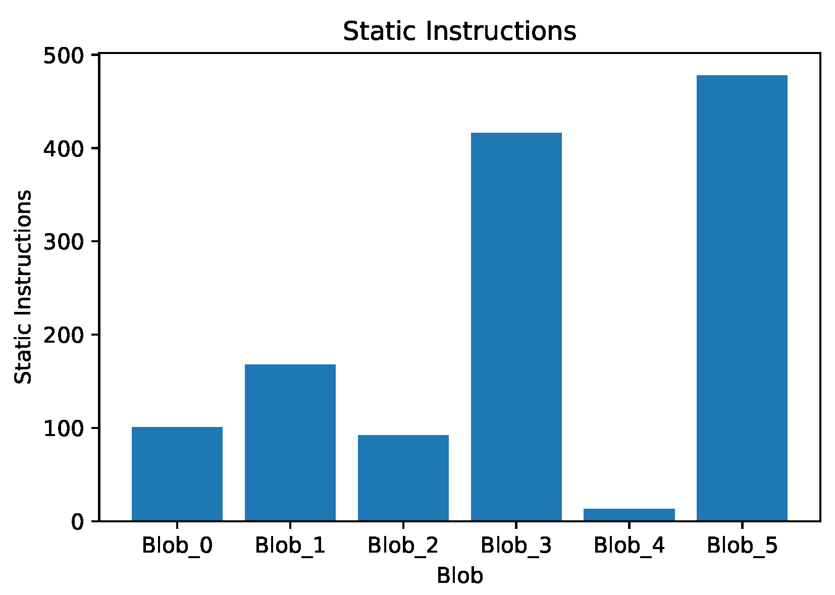
The natural loop blob creation algorithm (see sec:nat-loops-app) was executed on the STREAM benchmark, which generated 5 blobs. Blobs had an average of 211.3 static instructions per blob. Figure 13 shows blobs overlaid over the control flow graph. Functions are inlined in this representation, meaning each function call is represented by a unique set of nodes on the graph. Nodes with greater than 50 cache misses (the threshold value used in the algorithm) are highlighted in red.
Blobs were then dynamically analyzed using a program counter trace generated by Gem5 during the dynamic analysis phase. The trace contains an ordered list of all instruction addresses in the order they were executed, along with time stamps that allow synchronizing the program counter trace and the DRAM access trace. Dynamic analysis was able to confirm that in a non-anomalous run, program execution conformed to our blob-level graph (Figure 13).
Dynamic analysis was used to count the number of instructions that are executed in each blob access, as well as the total number of blob accesses and the order in which blob accesses occurred. Furthermore, a count of how many instructions are executed after entering a blob but before encountering a cache miss is tracked as an indicator of minimum latency a cache based classifier would encounter (See Table 1). This shows that the natural blob creation process has created relatively balanced blobs in terms of dynamic instruction – blobs 1-5 have over 100 million instructions dynamically executed but less than a billion instructions. Blob 0 is the entrance blob which has very few externally visible cache misses and very few executed instructions. Therefore, the bulk of the time is spent in relatively few blobs with few visits each. That is there is not a lot of switching between blobs that may cause noise in a monitor. Furthermore, the transitions between these blobs are within 410 thousand instructions or 0.17% of the start of the execution paths. Running at 1GHz or more, this would allow the lag of a monitor to be less than a millisecond in detection latency.
Figure 14.
Natural loops approach: static instruction counts per blob.
The SCC approach with dynamic profiling provides a larger number of blobs, ranging from 12 blobs up to 287 blobs for STREAM. However, even for the blob graph with the fewest number of blobs (a threshold of greater than two produces 12 blobs), execution often oscillates between several blobs resulting in the blobs being ineffective for coarsening the granularity of anomaly detection. Figure 15 shows a portion of such a blob graph highlighting a loop containing about 4.5 million LLC misses with each blob accounting for 1.5 million. While this balance would seem beneficial, inspection of the CFG and interleaving of the misses shows that the body of the loop has been broken up across different blobs resulting in interleaving of LLC misses at the granularity of a single LLC miss. Therefore, we use the natural loop approach for the remainder of our anomaly monitor evaluations.
6.3. Power Stream Blob Path Identification
In this experiment, our primary goal is to trace the execution flow of the STREAM benchmark through power-based side-channel information and report if it ever differs from the corresponding path in the golden model. We recorded 100 runs of the power side-channel information from the execution of STREAM benchmark for the golden path to build a machine learning model. The datasets are cleaned to remove the power samples collected during the program suspension interrupt handlers. These power sample sequences are labeled by the corresponding pathID. The pathID is determined using the PMU marker from benchmark’s blob entry for each blob. The PMU marker that emits the PMU counter values also associates the pathID of the blob path just traversed. The process of building a machine learning model is illustrated in Figure 16.
Feature extraction is an important step in any classification problem. This research prepares a train/test dataset with Fast Fourier Transform (FFT) followed by Principal Component Analysis (PCA). The power stream data often fails to synchronize across multiple runs due to irregular delay in interrupts. This causes a significant impact on classifying raw datasets. We convert the data into frequency domain and generate the feature vectors using PCA to avoid this. PCA is a well-known technique for dimensionality reduction. The supervised learning model’s size and efficiency such as SVM is severely affected by the feature vector size of the training dataset. PCA identifies and preserves the critical components of the feature vector with 95% variability in the FFT processed data, which helps to reduce the SVM model’s training complexity. The feature extraction techniques are applied separately on processor power and memory EM data to preserve their unique features. The feature vectors of processor and memory power data are concatenated for the given path to build the model. We use the Linear-SVM model to identify the blob/path execution localization in the benchmark.
In this work, we have built two different machine learning models on the recorded power stream datasets with the following objectives.
- Path-based Identification:
- The machine learning model is built to localize into a unique path through a blob that the benchmark executes.
- Blob-based Identification:
- The machine learning model is built to localize the execution into a blob in the benchmark.
Though we build two different models, the feature extraction steps are identical. The main difference in these models is based on the data used in training. In one case, targeting blob level identity, a power sample window at the beginning of a blob path concatenated with a power window at the end of a blob path constitutes the feature vector. In the other, a fixed size N-samples window slides over the sampled path to determine how likely is the power sample sequence to belong to that path.
Path-based Identification:
The datasets are parametrized with base parameters such as window width (W) and window separation (d). Since the benchmark execution takes several hours, the dataset is converted into multiple windows of width W separated from each other by d samples. This also reduces the host computer memory usage. For the given computational resources, the W and d are set to 1000000, which is illustrated in Figure 17. The constructed data is fed to the feature extractor PCA to compute unique feature values for processor power data and memory EM data. After PCA, the feature vector dimensions are reduced to 4590 from 1000000. The reduced feature vectors are concatenated to train the SVM model for unique pathIDs. The trained SVM model results in 81.7% accuracy on predicting the pathID. The saved model is used to trace the execution of the test run. The STREAM benchmark has nine unique paths, including the configuration steps. The PathID and have classification accuracy less than 50%, due to shorter execution paths compared to others. The and have lower number of memory accesses than other blobs. The PathID has the highest classification accuracy of 90%, whereas the accuracy of the remaining paths is between 70-80%.
The SVM-machine learning model is built to predict class variables as a token on the complete execution path of the benchmark along with the confidence values. There are 14056 tokens generated from the results of the ML model. We also computed the runs, a sequence of the same blob classification, of each class tokens along the execution path and plotted them in Figure 18. The x-axis defines the relative time calculated from the timestamp of the PX1500 interrupt marker. The y-axis represents the runs, the count of that blob classification, of each class token.
Blob-based Identification:
The datasets are constructed with the beginning and ending windows of power samples for each path. Each path datasets are in size as illustrated in Figure 19.
We built a power model using the new features obtained from the feature extractor in Figure 16. The model results in lower accuracy of around 55% to distinguish a blob. The lower accuracy may be caused by the noisy power samples from the programmable logic (PL) based Coherence client interrupts. Later, we recollected the power samples without PL interrupts and rebuilt a similar ML model. The new ML model results in % success rate on classifying the blobs.

Table 2.
Results on Blob-based Identification
| Blob-ID | Success rate |
|---|---|
| Blob-0 | 85% |
| Blob-1 | 96% |
| Blob-2 | 95% |
| Blob-3 | 86% |
| Blob-4 | 85% |
| Blob-5 | 90% |
6.4. Address Stream Blob Path Identification
A decision tree model was trained using an unlimited depth and unlimited number of leaf nodes. The model was trained using non-overlapping windows from a complete non-anomalous run. The model was tested against a second non-anomalous run, selecting 10K random windows as well as 100 random data windows from each class. The model ultimately produced an accuracy of 74.4%.
A confusion matrix (Figure 20) demonstrates high level of accuracy for individual blobs. However, attempts to classify transitions led to less accurate results as did differentiating between different paths. Blob accuracy is lower for smaller blobs and paths as well, notably seen in “Blob_0” and “Blob_32” (`Path_2’ through `Blob_3’).
6.5. PMU Stream Blob Path Identification
Two different PMU configurations are tested to achieve the highest accuracy. In the first configuration, PMU starts to count the number of events at the same time when the benchmark program starts. At each blob boundary, a PMU vector is generated with its corresponding path ID. We collect the data by running the benchmark 100 times to train an SVM linear machine learning model with half of the collected data (50 runs). The other half of the data is used to test the machine learning model accuracy. The SVM model can classify the testing data with 100% accuracy. During the experiment with a different configuration of the PMU, we noticed that the programmable logic interrupt and PX interrupt used to empty the buffers can affect the PMU counter values. This is because the PMU will continue counting the events during the interrupt. The interrupt handler is just an infinite event loop. It likely affects the total execution cycles event, but not many others. To reduce the noise in our PMU counter values, we tested another configuration where the PMU counter is stopped at entry into the program suspension interrupt handler. At the time, the PMU is stopped, the PMU counters are also reset to 0. The PMU will restart counting when the interrupt ends. This gives an abbreviated signature of the path segment from the last interrupt handler to the next blob. We performed the same machine learning experiment by dividing the data into two halves, one half for training and one half for testing. The machine learning results show that even by capturing a small path window at the path end, our SVM model can achieve 87% accuracy.
6.6. Monitor Blob Identification and Anomaly Detection
The Monitor is designed to check program state integrity at every blob transition boundary and along the paths within a blob at certain intervals. It does so by maintaining the known control flow paths of the program. This golden path model is checked against the current state of the program for anomalous behaviors. The current state of the program is determined by the unified decision from Power/EM, PMU and Address streams in the form of tokens generated by corresponding machine learning models. A token is a label uniquely identifying a blob/path. In a real time system, the blob/path token generation from the sampled program state will occur as a sublayer within the monitor by invoking the trained ML models.
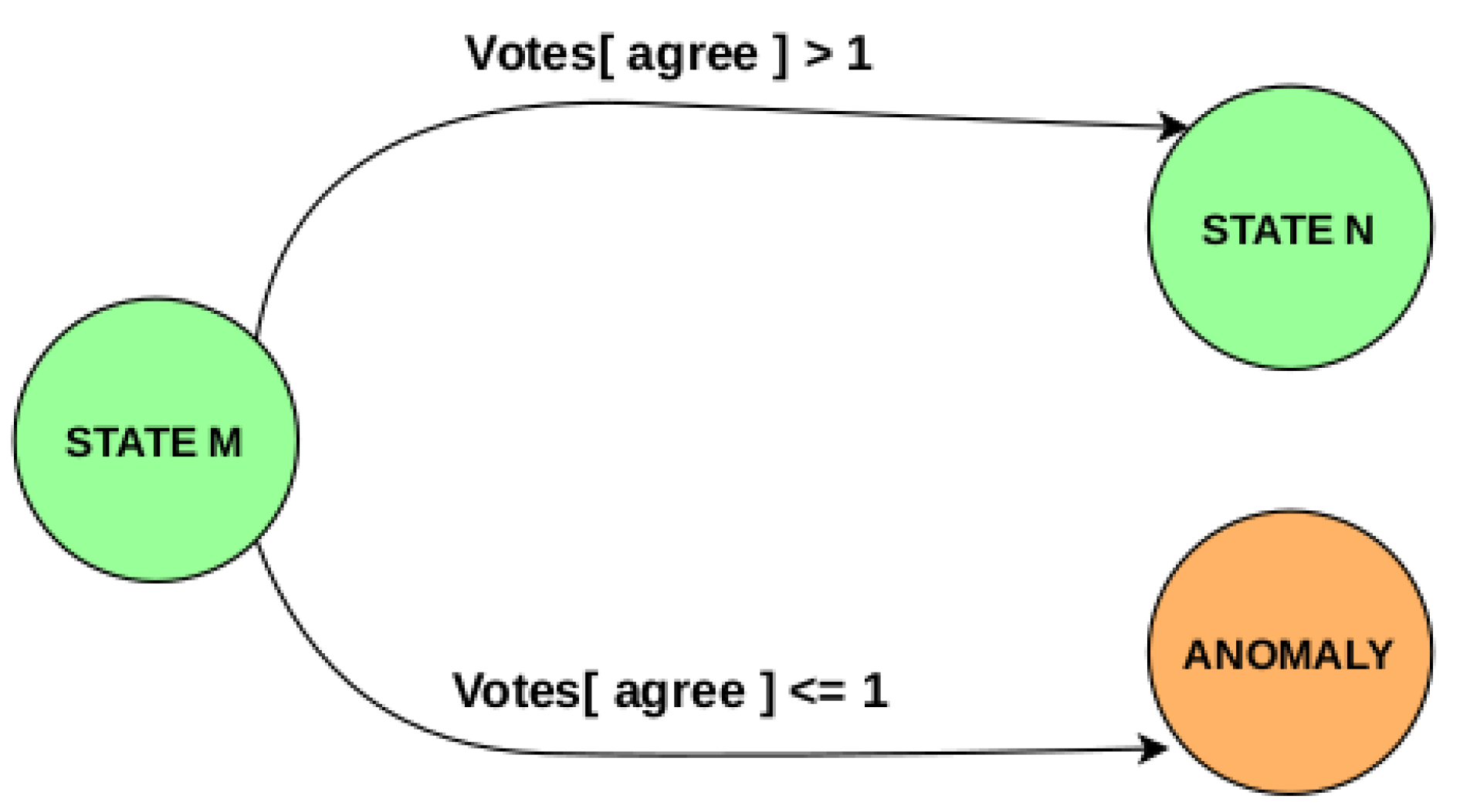
Figure 21.
State transition at Blob boundary.
Since the Monitor consumes tokens from three different streams, it is important to do so in a synchronized manner. Synchronization is done using a marker in the address stream that uniquely identifies when a PMU counter state is read. Power tokens are also aligned with this unique PMU marker. Since PMU counter state is read at blob boundaries, this technique synchronizes all the streams at every blob entry. Token consumption rate is also an important factor in keeping the three streams synchronized for the Monitor. PMU tokens are the most infrequent and are generated once per blob. Power tokens are generated at a fixed rate which is a function of the sampling frequency of the digitizer. Address token generation is irregular, driven by LLC activity. To allow synchronized token consumption, a counter is implemented within the FPGA logic (PL) that increments at every clock. Every address stream token is timestamped with this counter value. This gives us a sense of time elapsed in a blob in terms of PL clock. Power stream uses this notion of time to timestamp its own tokens, initializing at the address token timestamp at blob entry and incrementing every next token by a fixed amount determined by its sampling rate converted into PL clock domain.
The Monitor maintains its own clock that is initialized on entry to the first blob in the program. A token is consumed when its clock reaches the next closest timestamp value on a Power or Address token. This continues until the next blob entry at which point a PMU token is consumed.
In the current state of the Monitor, anomaly checks are performed at two granularities:
- At blob boundaries
- Along a path
On entering a new blob, the Monitor checks for anomalies based on PMU, Power and Address tokens consumed within the previous blob. If no anomalies are found, the current state is updated according to the golden model. This anomaly check involves a majority vote from the three streams. A token consumed within a blob may agree with the current state set by the golden model or it may disagree. We define a token as a goodToken if it agrees with the current state and a badToken as the one that disagrees. For Power and Address streams, the aggregate count of goodTokens and badTokens are used. A higher count of goodTokens within a blob than badTokens casts a vote in favor of the current state. For the single PMU token consumed at blob boundary, agreement with the current state casts a vote in favor of the current state. The Monitor then makes a transition to the next state as determined by the golden model if votes cast in favor of the current state exceeds 1. Else, it transitions to Anomaly state.
We test our Monitor on a subset of data collected for the 3 streams. We pick 3 datasets (labeled NR-12, NR-14, NR-17) that do not have an anomaly, and 2 datasets (MR-5, MR-9) that involve an anomaly. Figure 22, Figure 23 and Figure 24 show the test results. The first row represents the ground truth (golden model). For Figure 22, golden model is with respect to Blobs, while for Figure 23 it is with respect to Paths. The control flow of our test program (STREAM benchmark) when represented as Blobs, goes from Blob_0 to Blob_5 where Blob_3 has multiple entry/exit points and three internal paths. These are labeled as Blob_3_0, Blob_3_1, Blob_3_2. These form the columns in our results. Each row represents the vote from individual streams. Agree means that particular stream voted in favor of the current state. Disagree is a vote against the current state. The Monitor was tested on data collected from Blob_1 through Blob_5.
The control flow of the anomalous version of our test program goes to Blob_5 at the end, from Blob_1, bypassing Blob_3 and Blob_4. This is done by the CCI coherence fabric as well. For a preselected return address, it inserts another tampered address. Due to the anomaly, the control flow does not encounter a blob boundary from Blob_1 to Blob_5. The Monitor, therefore, sees it as a single blob. Thus the malicious results show a single vote for the two blobs traversed.
Figure 22 results show 4 out of 24 blobs mis-localized leading to an accuracy of for normal execution blob level localization. The anomalies are detected at 100% accuracy.
Anomaly checks are also done along a path. This is a more frequent check than the Blob transition boundary checks. In this approach, tokens received within a Blob are grouped into N-token sized windows. Within a single window, the number of goodTokens and badTokens are counted. This is done for every Blob/Path. The mean and standard deviation information of goodToken/badToken counts per window is extracted for each Blob/Path. During testing, the Monitor does a mean +/- K*standard-deviation () test to see if the current window passes this test. Failing to pass this test flags an anomaly. Figure 25 shows the results from this approach for Address stream. Window size of 2500 tokens were used. Results for the three datasets (NR-12, NR-14 and NR-17) are shown in each row. The numbers are the fraction of windows within a Blob/Path that passed the test. Blob_3_2 being a transition blob, has very few tokens and hence is not sufficiently large to form a full window. Results for that blob are not reported.
7. Discussion
Although, the assumption was that the decoupling of raw program state data collection and its analysis by the monitor into two steps to simplify this initial assessment effort, we did not foresee the additional difficulties this decomposition unleashes. Specifically,
- The synchronization between streams becomes extremely challenging through this decomposition. In a real-time system, synchronization can be built in implicitly or explicitly despite its challenging nature. But in the decomposed system model, as in this work, explicit crutches in terms of timestamps and markers have to be created.
- Misaligned raw data has a huge impact on blob/path detection accuracy further highlighting need for good synchronization.
The signals that are intentionally generated within a program - such as address stream and PMU, have higher fidelity than the unintentional side-channel signals such as power.
Based on our observations about the STREAM benchmark, complex backtracking at the monitor was not needed. But it is possible that as more complex programs with more complex control flow (blob flow) graphs are considered, more complex heuristics for backtracking may be needed at the monitor. It is also possible that we may not be able to localize at every blob with high accuracy for more complex benchmarks. However, we should be able to localize within one predecessor or successor blob of a blob with high accuracy for almost all benchmark programs.
The accuracy of many channels (such as PMU) is surprisingly high even if only a segment of an execution path is captured (). This offers interesting overhead-accuracy trade-offs opportunities.
For a completely decoupled monitor, using only the power stream, 70-80% accuracy seems to be achievable.
8. Conclusions
PCB embedded Trojans and hardware malware are a real threat to the computational integrity within a processor. In this research, we performed a preliminary assessment of a decoupled monitor, that observes the processor execution state at distance, mostly through side-channels and memory address channels - the attributes naturally visible outside a processor boundary.
Control flow integrity at the granularity of an aggregated control flow graph into blobs can be monitored by such a decoupled monitor. Based on the resources allocated to such a monitor, blobs sizes can be tailored by the compiler - providing a rich performance-accuracy trade-off. Our results show that with a multi-modal sensor stream, the location of the execution or control flow within a control flow graph can be accurately pinpointed by a decoupled monitor with accuracy in the range 80-90%. Anomalous control flow was detected with 100% accuracy.
A real-time prototype unifying data collection, analysis, and decision making will pose challenges in the real time aspects. The analysis through machine learning will be challenging based on the period of the analysis. In our current implementation, the address stream analysis occurs every time an LLC miss address is found. The average separation between LLC addresses seems to be 200-300 clock cycles. Building an SVM engine with 200-300 processor clock cycles latency is feasible. It will involve various trade-offs between feature vector size, efficiency of SVM classification, and the processor clock frequency. We believe that better synchronization afforded by a real-time system can boost the accuracy. This may be offset by the real time considerations (reduced feature vector size in order to perform ML classification in 200-300 clock cycles) to bring back the overall accuracy in the 80-90% range.
Two spaces exist for this kind of anomaly monitor - one where the execution design and program source code are within the end-user control, and the other where the execution engine and the program are black boxes. The former design point exemplified by an SoC with in-house embedded transactional programs is a better-suited candidate for such a decoupled monitor. Such a platform may even offer other explicitly inserted high-fidelity event channels (such as interrupts) leading to even higher monitoring accuracy. The latter design point relies primarily on the power side-channel as the main indicator which can still lead to over 80% accuracy.
Author Contributions
Henry Duwe and Akhilesh Tyagi conceptualized this project with Henry Duwe leading the blob level conceptualization and Akhilesh Tyagi leading the side-channel conceptualization. They are also responsible for funding acquisition. Ananda Biswas implemented PMU based side-channel and the decoupled monitor. Dakota Berbrich contributed to SCC blob heuristics and implementation. Braedon Giblin had primary responsibility for blob implementation. Zelong Li supported compiler level event insertion and machine learning efforts. Ravikumar Selvam built the power and EM side-channel infrastructure. Joyesh Philip provided board level engineering and cache coherence address stream collection support. and anomalous cache trigger insertion. All of the authors have read and agreed to the published version of the manuscript.
Funding
This research was supported by Defense Advanced Research Projects Agency through contract DARPA/IA DESTRO FA8750-20-1-0504.
Institutional Review Board Statement
Not applicable.
Informed Consent Statement
Not applicable.
Data Availability Statement
The original contributions presented in this study are included in the article. Further inquiries can be directed to the corresponding author(s).
Abbreviations
| PMU | Performance Monitoring Unit |
| CFI | Control Flow Integrity |
| LLC | Last Level Cache |
| DDR | Double Data Rate |
| FPGA | Field Programmable Gate Array |
| CFG | Control Flow Graph |
| BFG | Blob Flow Graph |
| LLVM | Low Level Virtual Machine |
| COTS | Commercial Off The Shelf |
| PL | Programmable Logic |
| CCI | Cache Coherence Interface |
| L1D | Level-1 Data Cache |
| L1I | Level-1 Instruction Cache |
| ML | Machine Learning |
| EM | Electromagnetic |
| PESI | Program Execution State Integrity |
| PCB | Printed Circuit Board |
| PCA | Principal Component Analysis |
| SCA | Side-Channel Attack |
References
- Wikipedia. Trusted Foundry Program. Available online: https://en.wikipedia.org/wiki/Trusted_Foundry_Program.
- Rajendran, J.; Sinanoglu, O.; Karri, R. Regaining Trust in VLSI Design: Design-for-Trust Techniques. Proceedings of the IEEE 2014, 102, 1266–1282. [Google Scholar] [CrossRef]
- Vaarandi, R.; Tsiopoulos, L.; Visky, G.; ur Rehman, M.; Bahsi, H. A Systematic Literature Review of Cyber Security Monitoring in Maritime. IEEE Access 2025, 13, 85307–85329. [Google Scholar] [CrossRef]
- Diana, L.; Dini, P.; Paolini, D. Overview on Intrusion Detection Systems for Computers Networking Security. Computers 2025, 14. [Google Scholar] [CrossRef]
- Park, J.; Xu, X.; Jin, Y.; Forte, D.; Tehranipoor, M. Power-based side-channel instruction-level disassembler. In Proceedings of the Proceedings of the 55th Annual Design Automation Conference, DAC ’18. New York, NY, USA, 2018. [Google Scholar] [CrossRef]
- Krishnankutty, D.; Li, Z.; Robucci, R.; Banerjee, N. Instruction Sequence Identification and Disassembly Using Power Supply Side-Channel Analysis. IEEE Transactions on Computers 2020, 69, 1639–1651. [Google Scholar] [CrossRef]
- Fendri, H.; Macchetti, M.; Perrine, J.; Stojilović, M. A deep-learning approach to side-channel based CPU disassembly at design time. In Proceedings of the Proceedings of the 2022 Conference & Exhibition on Design, Automation & Test in Europe, Leuven, BEL, 2022; DATE ’22, pp. 670–675. [Google Scholar]
- Glamočanin, O.; Shrivastava, S.; Yao, J.; Ardo, N.; Payer, M.; Stojilović, M. Instruction-Level Power Side-Channel Leakage Evaluation of Soft-Core CPUs on Shared FPGAs. In Proceedings of the Proceedings of the 32nd USENIX Security Symposium, 2023; pp. 2926–2944. [Google Scholar]
- Brisfors, M.; Moraitis, M.; Dubrova, E. Do Not Rely on Clock Randomization: A Side-Channel Attack on a Protected Hardware Implementation of AES. In Proceedings of the Foundations and Practice of Security: 15th International Symposium, FPS 2022, Ottawa, ON, Canada; Revised Selected Papers, Berlin, Heidelberg, December 12–14, 2022; pp. 38–53. [Google Scholar] [CrossRef]
- Uhsadel, L.; Georges, A.; Verbauwhede, I. Exploiting hardware performance counters. In Proceedings of the 2008 5th Workshop on Fault Diagnosis and Tolerance in Cryptography, 2008; IEEE; pp. 59–67. [Google Scholar]
- Biswas, A.; Li, Z.; Tyagi, A. Control Flow Integrity in IoT Devices with Performance Counters and DWT. In Proceedings of the 2020 IEEE International Symposium on Smart Electronic Systems (iSES) (Formerly iNiS), 2020; pp. 171–176. [Google Scholar] [CrossRef]
- Malone, C.; Zahran, M.; Karri, R. Are hardware performance counters a cost effective way for integrity checking of programs. In Proceedings of the Proceedings of the Sixth ACM Workshop on Scalable Trusted Computing, New York, NY, USA, 2011; STC ’11, pp. 71–76. [Google Scholar] [CrossRef]
- Xia, Y.; Liu, Y.; Chen, H.; Zang, B. CFIMon: Detecting violation of control flow integrity using performance counters. In Proceedings of the IEEE/IFIP International Conference on Dependable Systems and Networks (DSN 2012), 2012; pp. 1–12. [Google Scholar] [CrossRef]
- Kocher, P.C.; Jaffe, J.; Jun, B. Differential Power Analysis. In Proceedings of the Advances in Cryptology - CRYPTO ’99, 19th Annual International Cryptology Conference, Santa Barbara, California, USA; Proceedings, August 15-19, 1999; 1999; pp. 388–397. [Google Scholar] [CrossRef]
- Kocher, P.C. Timing Attacks on Implementations of Diffie-Hellman, RSA, DSS, and Other Systems. In Proceedings of the Advances in Cryptology — CRYPTO ’96; Berlin, Heidelberg, Koblitz, N., Ed.; 1996; pp. 104–113. [Google Scholar]
- Quisquater, J.J.; Samyde, D. Electromagnetic analysis (ema): Measures and counter-measures for smart cards. In Proceedings of the International Conference on Research in Smart Cards, 2001; Springer; pp. 200–210. [Google Scholar]
- Genkin, D.; Pipman, I.; Tromer, E. Get Your Hands Off My Laptop: Physical Side-Channel Key-Extraction Attacks on PCs. In Proceedings of the Cryptographic Hardware and Embedded Systems – CHES 2014; Berlin, Heidelberg, Batina, L., Robshaw, M., Eds.; 2014; pp. 242–260. [Google Scholar]
- Eisenbarth, T.; Paar, C.; Weghenkel, B. Building a side channel based disassembler. In Transactions on Computational Science X: Special Issue on Security in Computing, Part I; Springer-Verlag: Berlin, Heidelberg, 2010; pp. 78–99. [Google Scholar]
- Park, J.; Tyagi, A. Security Metrics for Power Based SCA Resistant Hardware Implementation. In Proceedings of the Proceedings of the 2016 29th International Conference on VLSI Design and 2016 15th International Conference on Embedded Systems (VLSID), USA, 2016; VLSID ’16, pp. 541–546. [Google Scholar] [CrossRef]
- Park, J.; Tyagi, A. Using Power Clues to Hack IoT Devices: The power side channel provides for instruction-level disassembly. IEEE Consumer Electronics Magazine 2017, 6, 92–102. [Google Scholar] [CrossRef]
- Robins, A.; Olguin, S.; Brown, J.; Carper, C.; Borowczak, M. Power-Based Side-Channel Attacks on Program Control Flow with Machine Learning Models. Journal of Cybersecurity and Privacy 2023, 3, 351–363. [Google Scholar] [CrossRef]
- Han, Y.; Chan, M.; Aref, Z.; Tippenhauer, N.O.; Zonouz, S. Hiding in Plain Sight? On the Efficacy of Power Side Channel-Based Control Flow Monitoring. In Proceedings of the 31st USENIX Security Symposium (USENIX Security 22), Boston, MA, 2022; pp. 661–678. [Google Scholar]
- Vaidyan, V.M.; Tyagi, A. Instruction Level Disassembly through Electromagnetic Side-Chanel: Machine Learning Classification Approach with Reduced Combinatorial Complexity. In Proceedings of the Proceedings of the 2020 3rd International Conference on Signal Processing and Machine Learning, New York, NY, USA, 2020; SPML ’20, pp. 124–130. [Google Scholar] [CrossRef]
- Arguello, C.N.; Searle, H.; Rampazzi, S.; Butler, K.R.B. A Practical Methodology for ML-Based EM Side Channel Disassemblers. arXiv 2022, arXiv:2206.10746. [Google Scholar] [CrossRef]
- Maillard, J.; Hiscock, T.; Lecomte, M.; Clavier, C. Towards Fine-grained Side-Channel Instruction Disassembly on a System-on-Chip. In Proceedings of the 2022 25th Euromicro Conference on Digital System Design (DSD), 2022; pp. 472–479. [Google Scholar] [CrossRef]
- van Geest, J.; Buhan, I. A Side-Channel Based Disassembler for the ARM-Cortex M0. In Proceedings of the Applied Cryptography and Network Security Workshops: ACNS 2022 Satellite Workshops, AIBlock, AIHWS, AIoTS, CIMSS, Cloud S&P, SCI, SecMT, SiMLA, Rome, Italy; Proceedings, Berlin, Heidelberg, June 20–23, 2022; pp. 183–199. [Google Scholar] [CrossRef]
- Iyer, V.V.; Thimmaiah, A.; Orshansky, M.; Gerstlauer, A.; Yilmaz, A.E. A Hierarchical Classification Method for High-accuracy Instruction Disassembly with Near-field EM Measurements. ACM Trans. Embed. Comput. Syst. 2024, 23. [Google Scholar] [CrossRef]
- Callan, R.; Behrang, F.; Zajic, A.; Prvulovic, M.; Orso, A. Zero-overhead profiling via EM emanations. In Proceedings of the Proceedings of the 25th International Symposium on Software Testing and Analysis, New York, NY, USA, 2016; ISSTA 2016, pp. 401–412. [Google Scholar] [CrossRef]
- Sayakkara, A.; Le-Khac, N.A.; Scanlon, M. A survey of electromagnetic side-channel attacks and discussion on their case-progressing potential for digital forensics. Digit. Investig. 2019, 29, 43–54. [Google Scholar] [CrossRef]
- Han, Y.; Christoudis, I.; Diamantaras, K.I.; Zonouz, S.; Petropulu, A. Side-Channel-Based Code-Execution Monitoring Systems: A Survey. IEEE Signal Processing Magazine 2019, 36, 22–35. [Google Scholar] [CrossRef]
- Aho, A.V.; Lam, M.S.; Sethi, R.; Ullman, J.D. Compilers: Principles, Techniques, and Tools (2nd Edition); Addison-Wesley Longman Publishing Co., Inc.: USA, 2006. [Google Scholar]
- Mahlke, S.; Lin, D.; Chen, W.; Hank, R.; Bringmann, R. Effective Compiler Support For Predicated Execution Using The Hyperblock. In Proceedings of the [1992] Proceedings the 25th Annual International Symposium on Microarchitecture MICRO 25, 1992; pp. 45–54. [Google Scholar] [CrossRef]
- Fisher, J.A. Trace Scheduling: A Technique for Global Microcode Compaction. IEEE Transactions on Computers 1981, C-30, 478–490. [Google Scholar] [CrossRef]
- Lokuciejewski, P.; Kelter, T.; Marwedel, P. Superblock-Based Source Code Optimizations for WCET Reduction. In Proceedings of the Proceedings of the 2010 10th IEEE International Conference on Computer and Information Technology, USA, 2010; CIT ’10, pp. 1918–1925. [Google Scholar] [CrossRef]
- Zhang, Y. Cache Side Channels: State of the Art and Research Opportunities. In Proceedings of the Proceedings of the 2017 ACM SIGSAC Conference on Computer and Communications Security, New York, NY, USA, 2017; CCS ’17, pp. 2617–2619. [Google Scholar] [CrossRef]
- Aldaya, A.C.; Brumley, B.B.; ul Hassan, S.; Pereida García, C.; Tuveri, N. Port Contention for Fun and Profit. In Proceedings of the 2019 IEEE Symposium on Security and Privacy (SP), 2019; pp. 870–887. [Google Scholar] [CrossRef]
- Rokicki, T.; Maurice, C.; Botvinnik, M.; Oren, Y. Port Contention Goes Portable: Port Contention Side Channels in Web Browsers. In Proceedings of the Proceedings of the 2022 ACM on Asia Conference on Computer and Communications Security, New York, NY, USA, 2022; ASIA CCS ’22, pp. 1182–1194. [Google Scholar] [CrossRef]
- Li, X.; Tyagi, A. Multi-Line Prefetch Covert Channel with Huge Pages. Cryptography 2025, 9. [Google Scholar] [CrossRef]
- LLVM. The LLVM Compiler Infrastructure. Available online: https://llvm.org/.
- Gem5. Gem5: The Gem5 Simulator System. Available online: https://www.gem5.org/.
- Binkert, N.; Beckmann, B.; Black, G.; Reinhardt, S.K.; Saidi, A.; Basu, A.; Hestness, J.; Hower, D.R.; Krishna, T.; Sardashti, S.; et al. The gem5 simulator. SIGARCH Comput. Archit. News 2011, 39, 1–7. [Google Scholar] [CrossRef]
- Sharir, M. A strong-connectivity algorithm and its applications in data flow analysis. Computers & Mathematics with Applications 1981, 7, 67–72. [Google Scholar] [CrossRef]
- Xilinx. Xilinx ZCU 106 Evaluation Board User Guide. 23 October 2019, UG1244. Available online: https://www.xilinx.com/support/documentation/boards_and_kits/zcu106/ug1244-zcu106-eval-bd.pdf.
- ARM. Arm Cortex-A53 MPCore Processor Technical Reference Manual. Available online: https://developer.arm.com/documentation/ddi0500/latest/.
- McCalpin, J. STREAM Benchmark Git. Available online: https://www.cs.virginia.edu/stream/.
- Hammond, J. STREAM: Sustainable Memory Bandwidth in High Performance Computers. Available online: https://github.com/jeffhammond/STREAM.
| 1 | Note that this methodology fits in well with the plans of LLVM [39] to provide CFG information along with assembly program for the purpose of link-time assembly code optimizations. |
| 2 | Although the memory-access stream is directly collected on-chip, L2 misses are visible off-chip via the DDR bus. |
Figure 1.
Monitor Overview
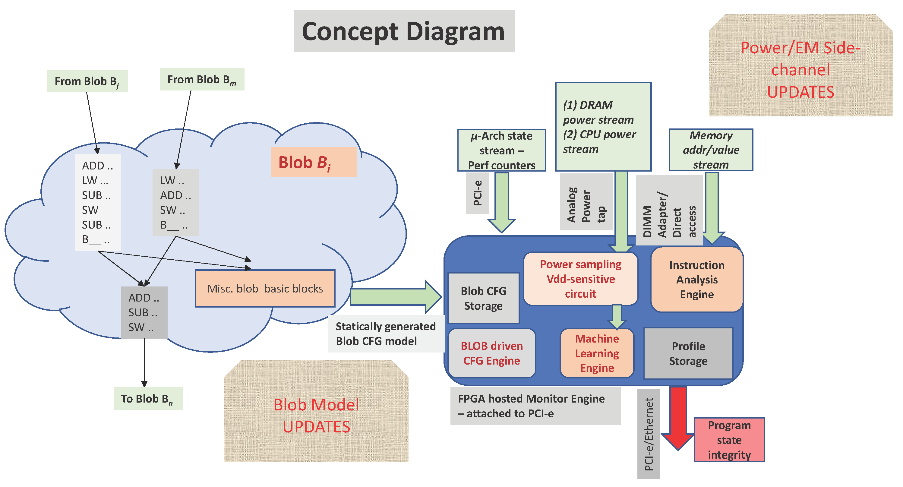
Figure 2.
Blob and Basic Blocks
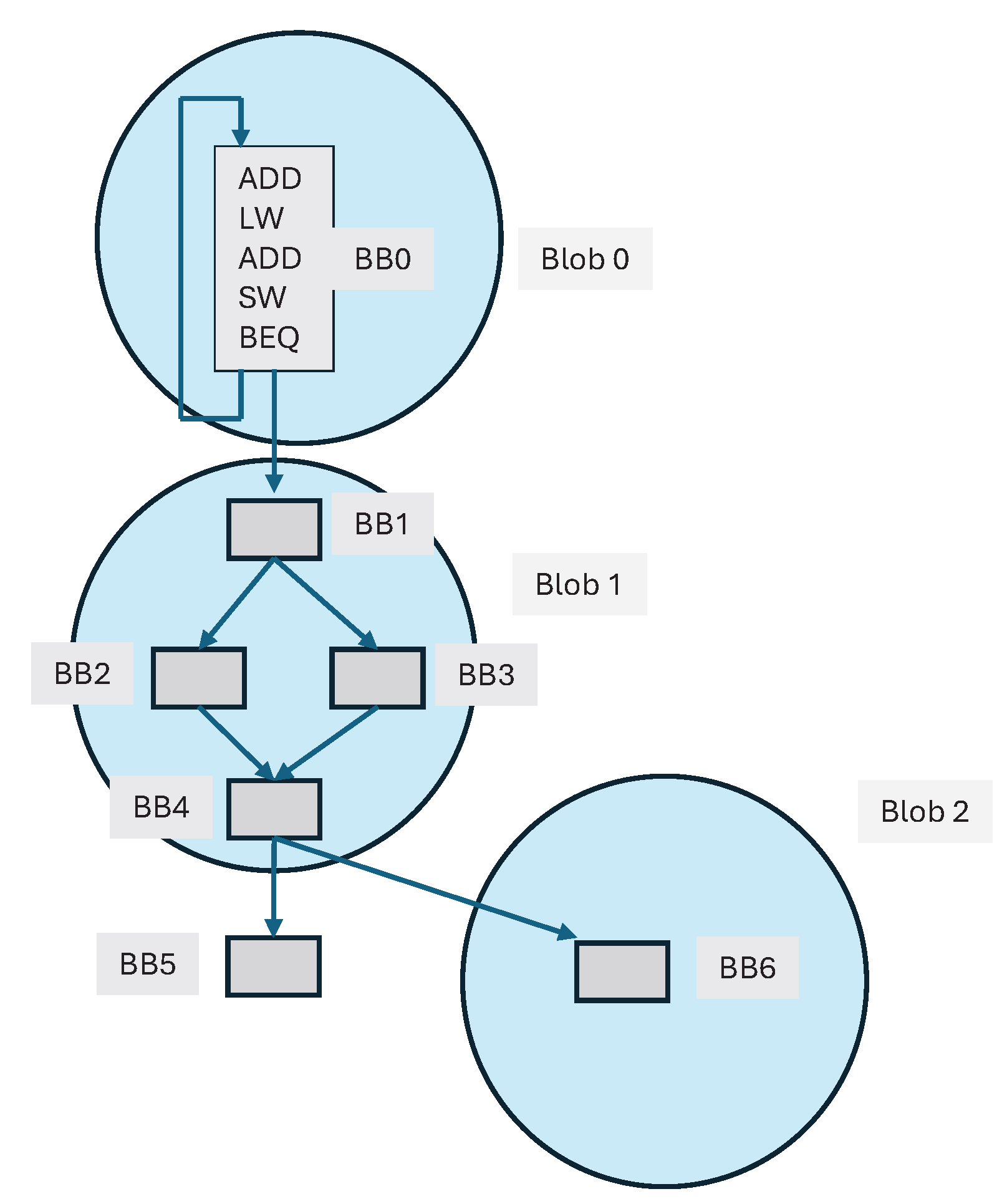
Figure 3.
Blob creation process
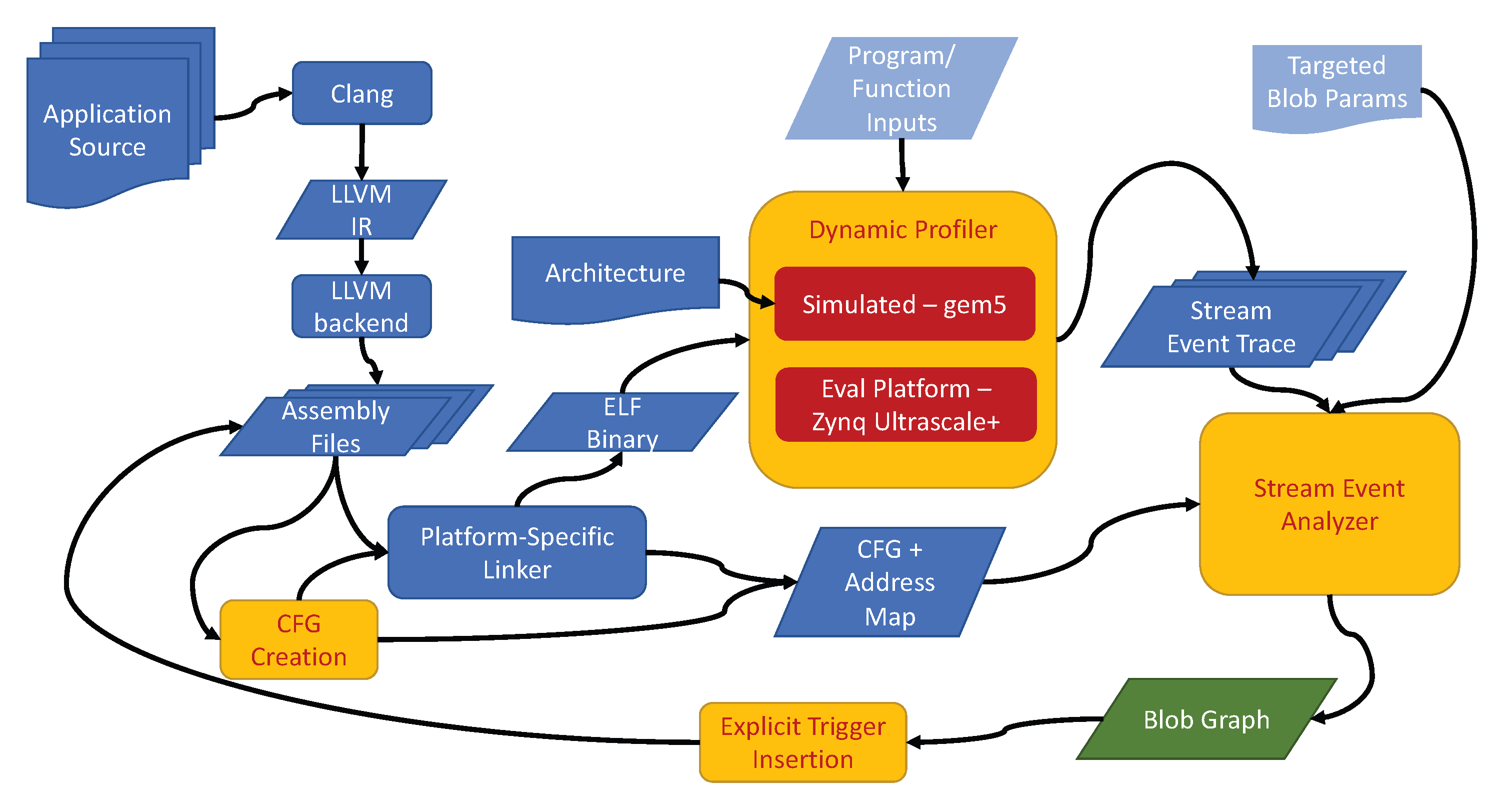
Figure 4.
Blob graph naively constructed from profiling.
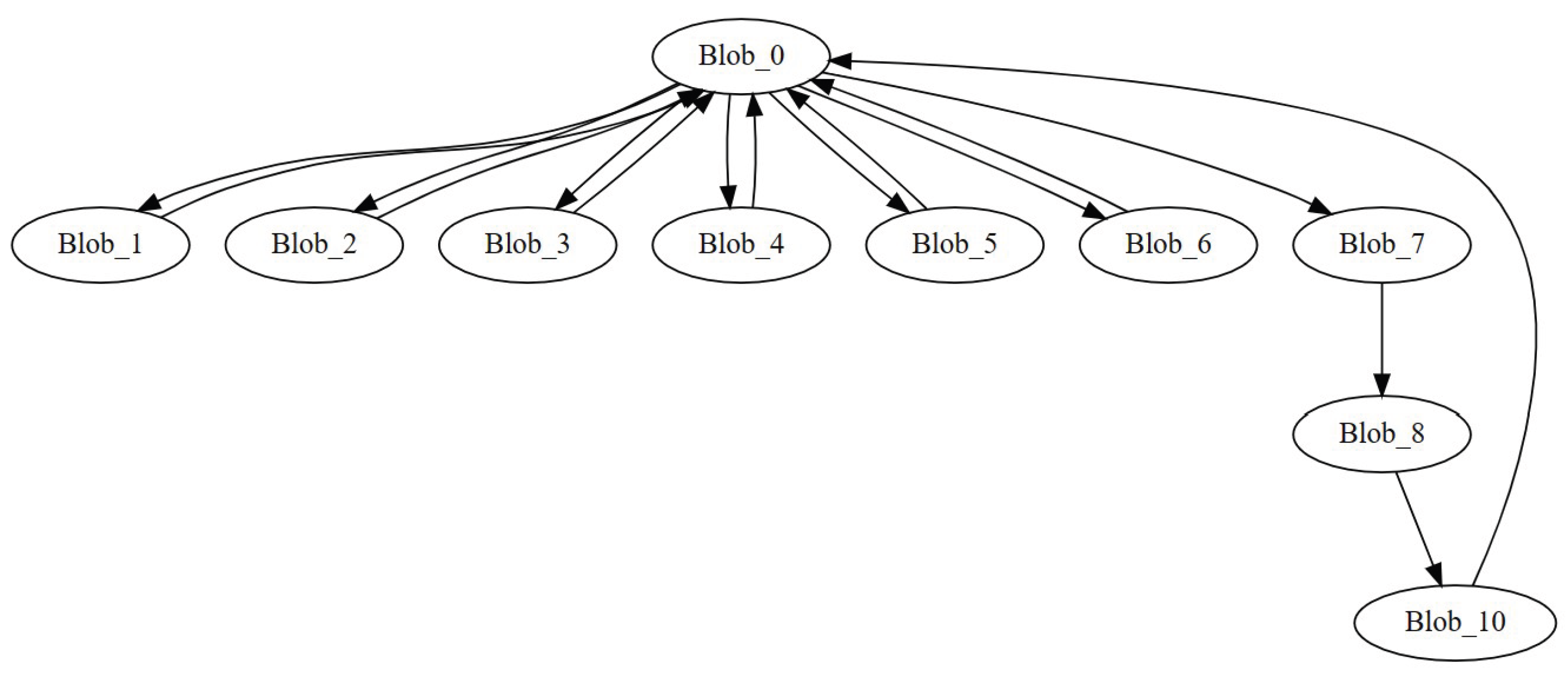
Figure 5.
Xilinx Zynq Ultrascale+ ZCU106 evaluation platform showing the quad core ARM Cortex A53 application processor, the Cortex R5 subsystem, the multi-level cache and interconnect hierarchy, the programmable logic fabric, and the external DDR memory interface that together define the core architecture of the system [43].
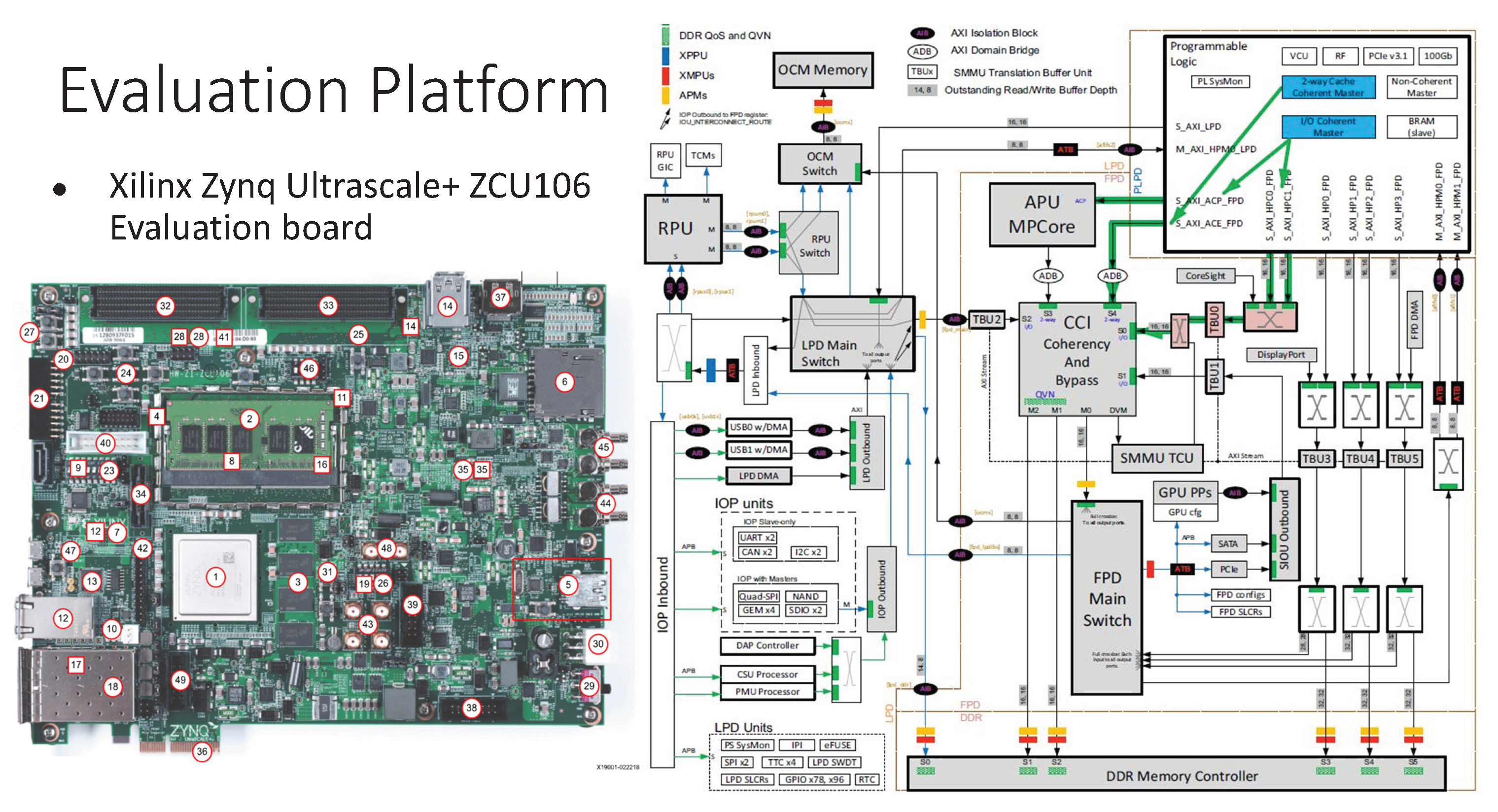
Figure 6.
Processor and DDR power domains on the ZCU106 board, showing independently monitored supply paths and the parallel capacitor network used to stabilize each domain.
Figure 6.
Processor and DDR power domains on the ZCU106 board, showing independently monitored supply paths and the parallel capacitor network used to stabilize each domain.
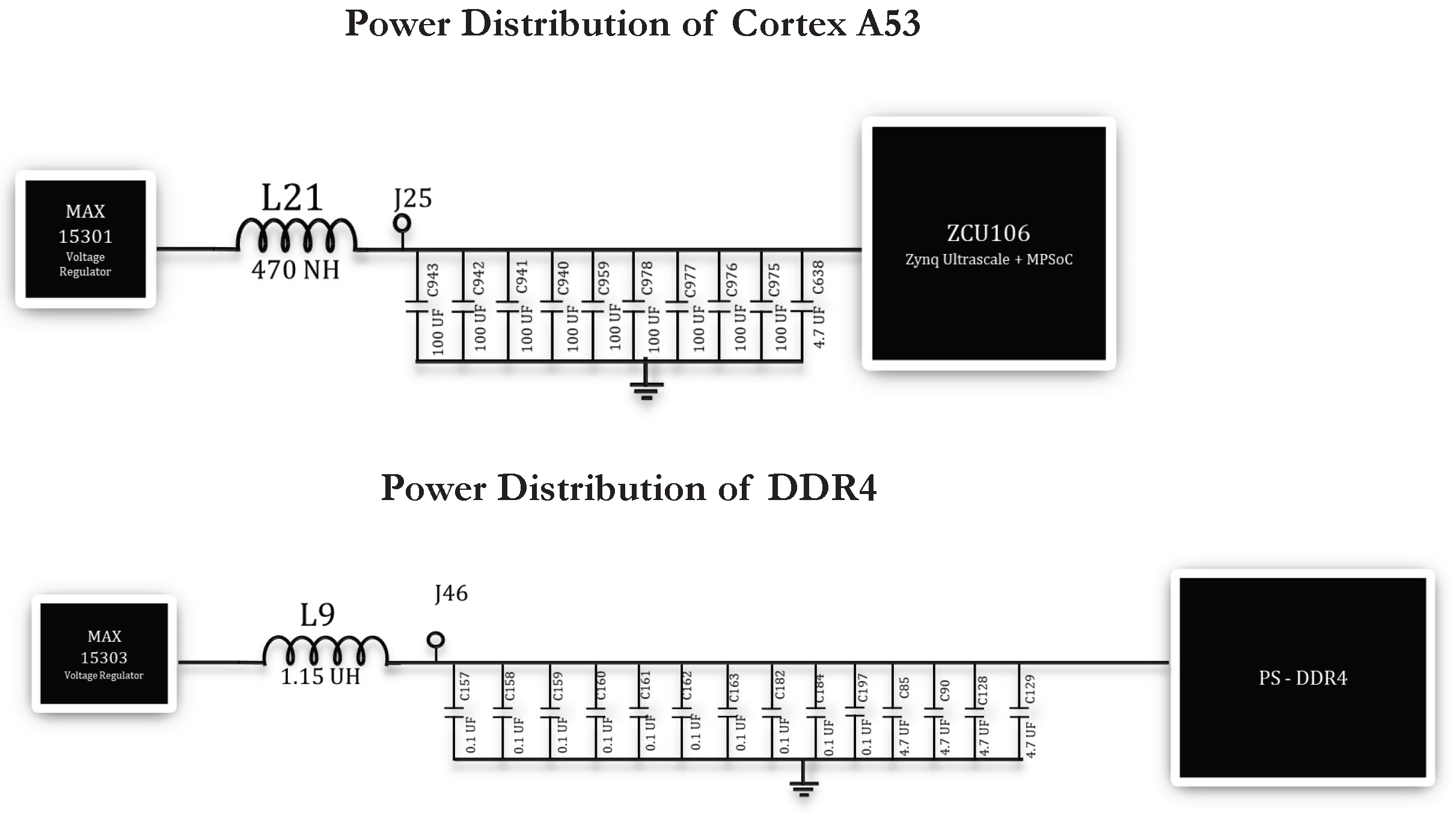
Figure 7.
Custom PCB design integrating the full capacitor bank and a dedicated shunt-resistance interface, designed to maintain stable power delivery while enhancing observability.
Figure 7.
Custom PCB design integrating the full capacitor bank and a dedicated shunt-resistance interface, designed to maintain stable power delivery while enhancing observability.
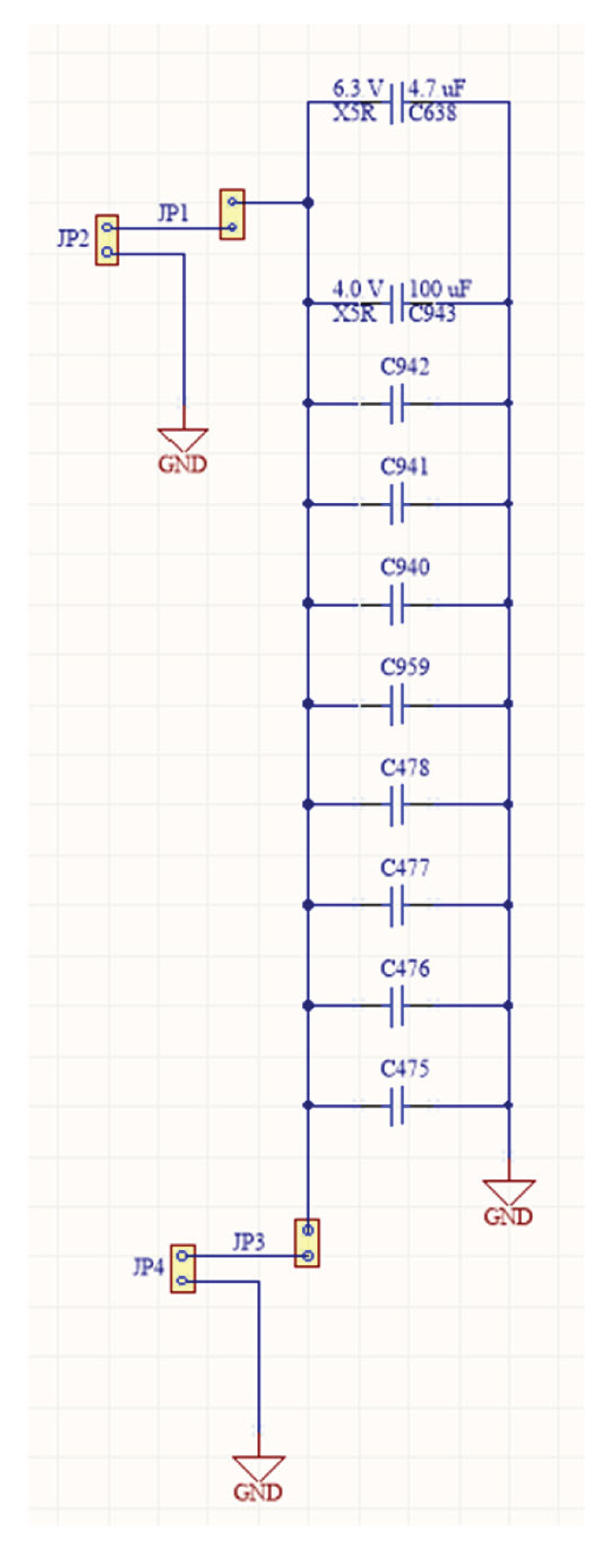
Figure 8.
Dual-channel acquisition setup: Channel 1 captures processor power, and Channel 2 captures DDR EM emissions via a TBPS01 probe connected to the PX1500 digitizer.
Figure 8.
Dual-channel acquisition setup: Channel 1 captures processor power, and Channel 2 captures DDR EM emissions via a TBPS01 probe connected to the PX1500 digitizer.
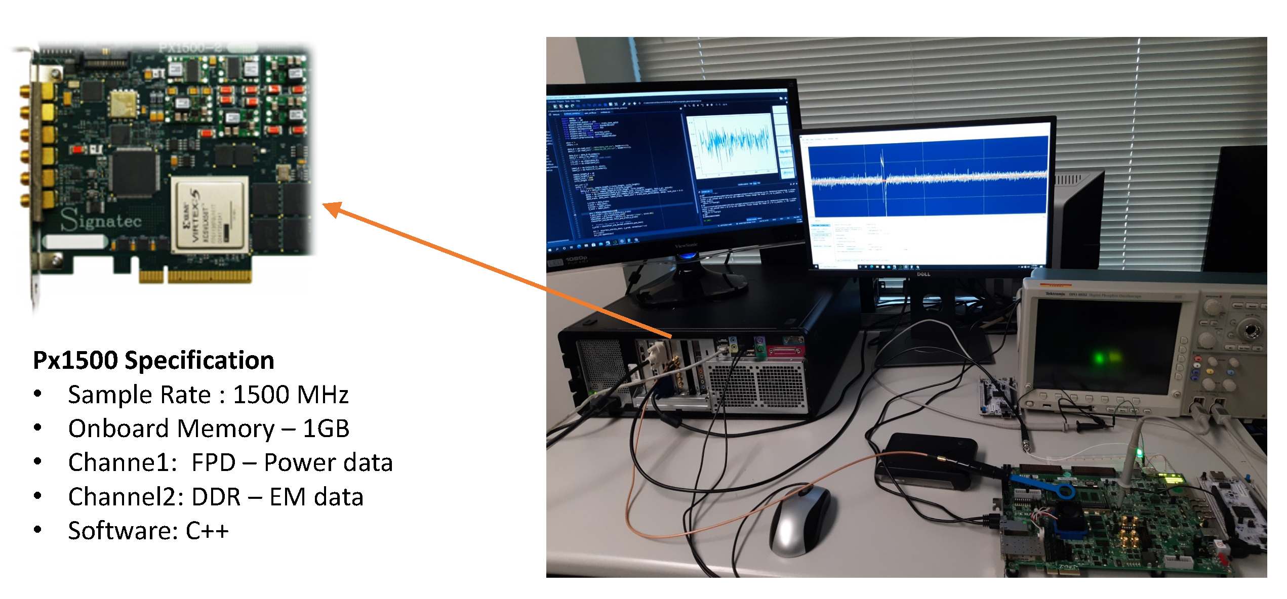
Figure 9.
Simultaneous processor-power and DDR-domain EM waveforms showing correlated activity during a memory-access event. The alignment of features across both traces highlights the visibility of microarchitectural behavior.
Figure 9.
Simultaneous processor-power and DDR-domain EM waveforms showing correlated activity during a memory-access event. The alignment of features across both traces highlights the visibility of microarchitectural behavior.
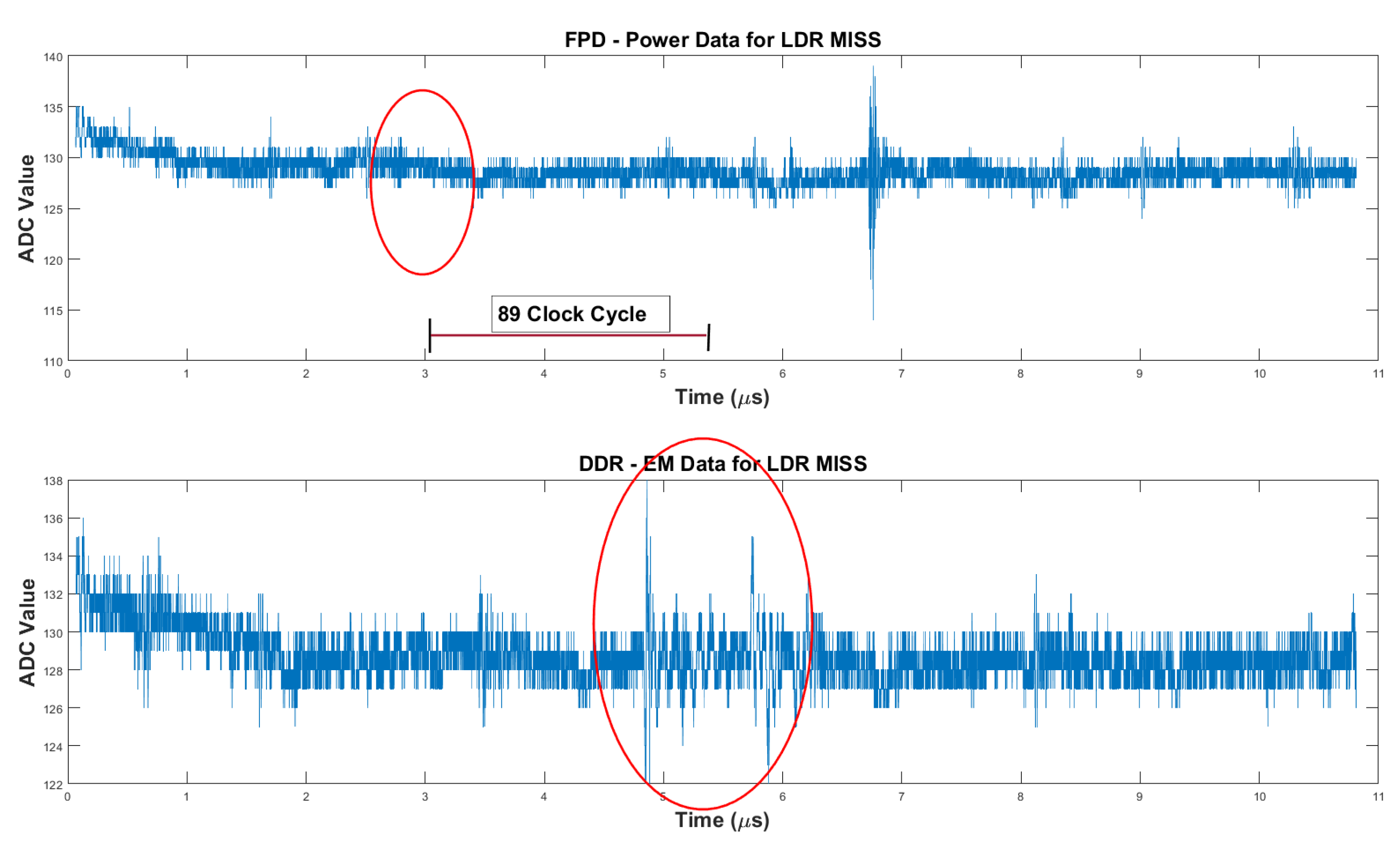
Figure 10.
Coherent Cache Interface for Address Stream Collection
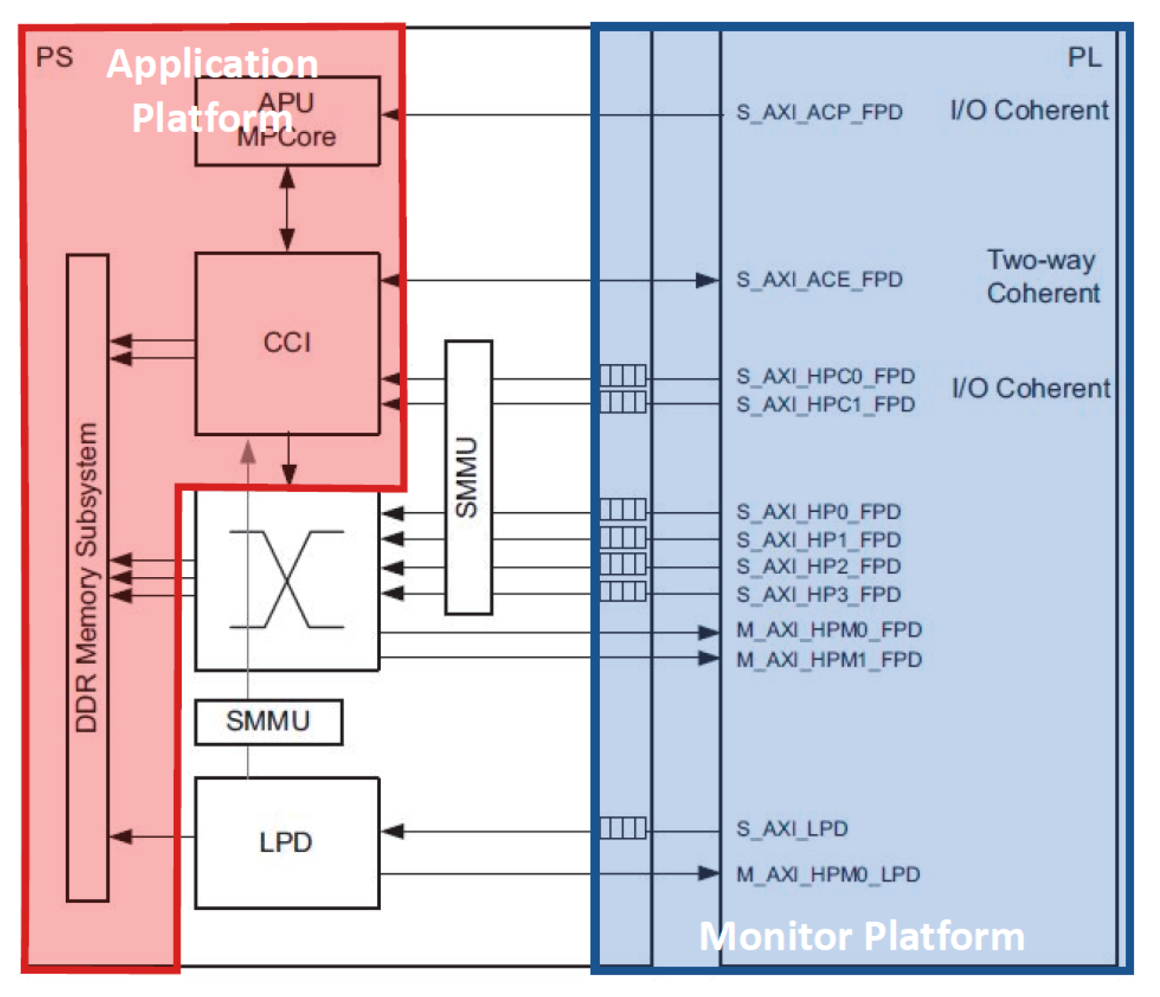
Figure 11.
Example Stream benchmark address trace.
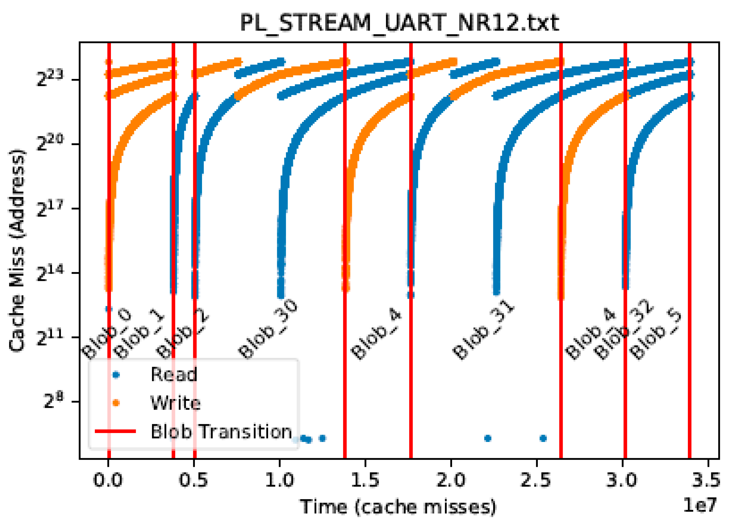
Figure 12.
Raw Data Collection Phase for LLC Miss, Power/EM, PMU Data
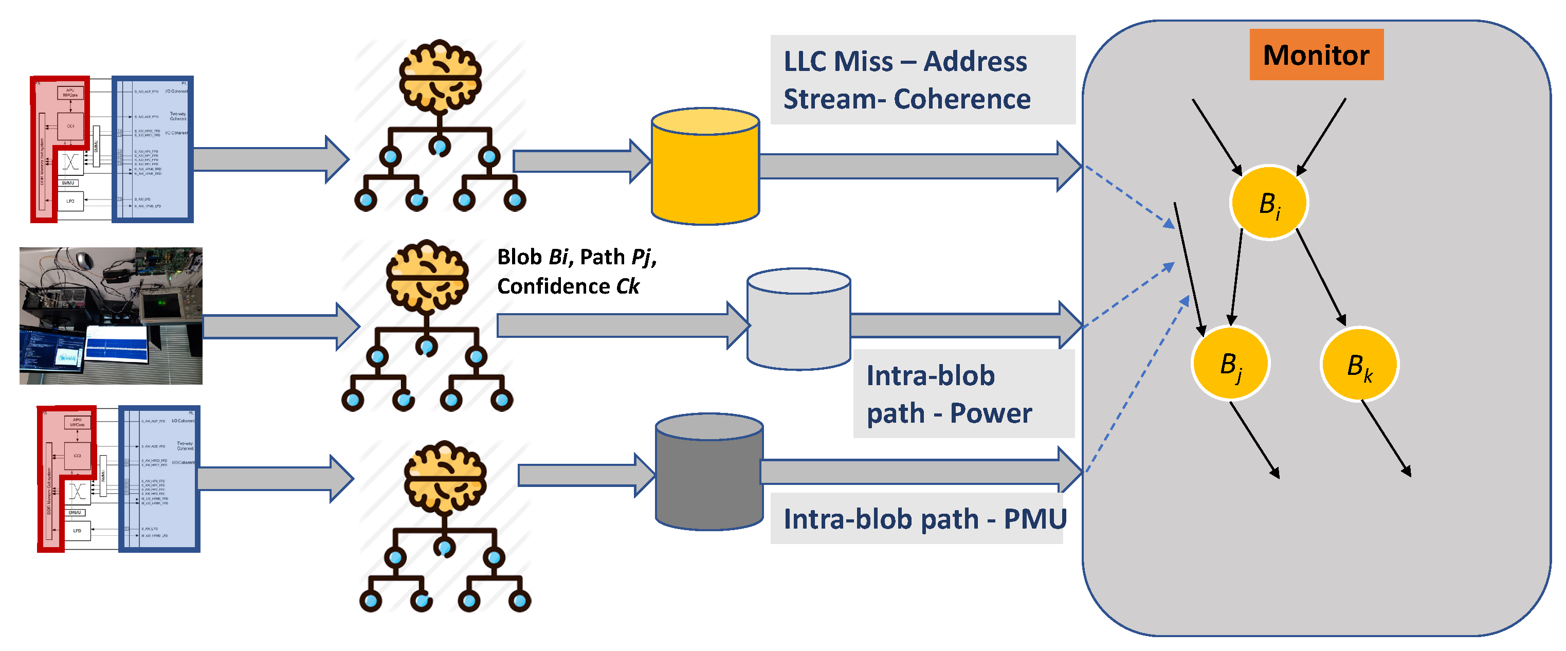
Figure 13.
Natural loops approach: blob level graph
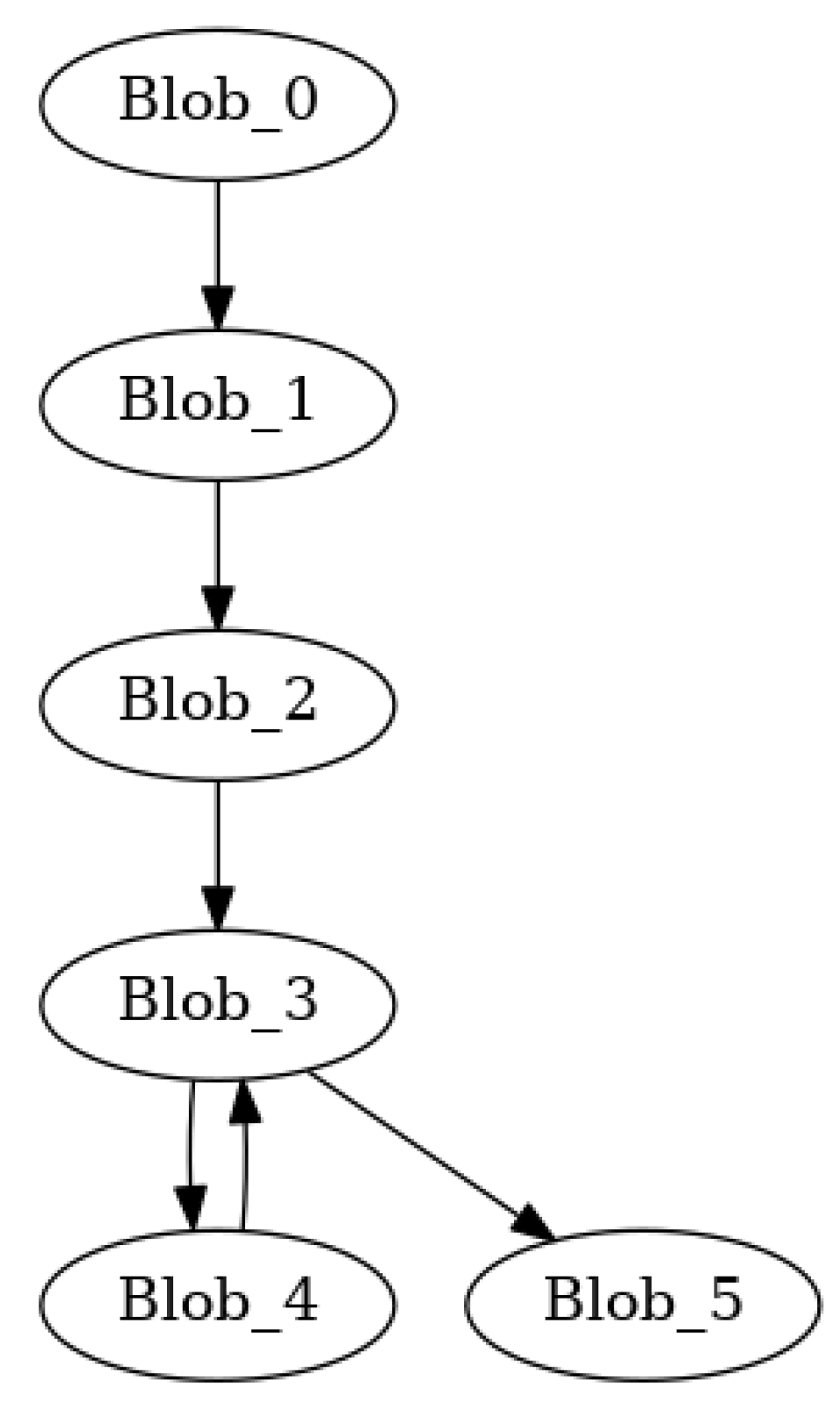
Figure 15.
SCC approach with dynamic profiling: blob level graph
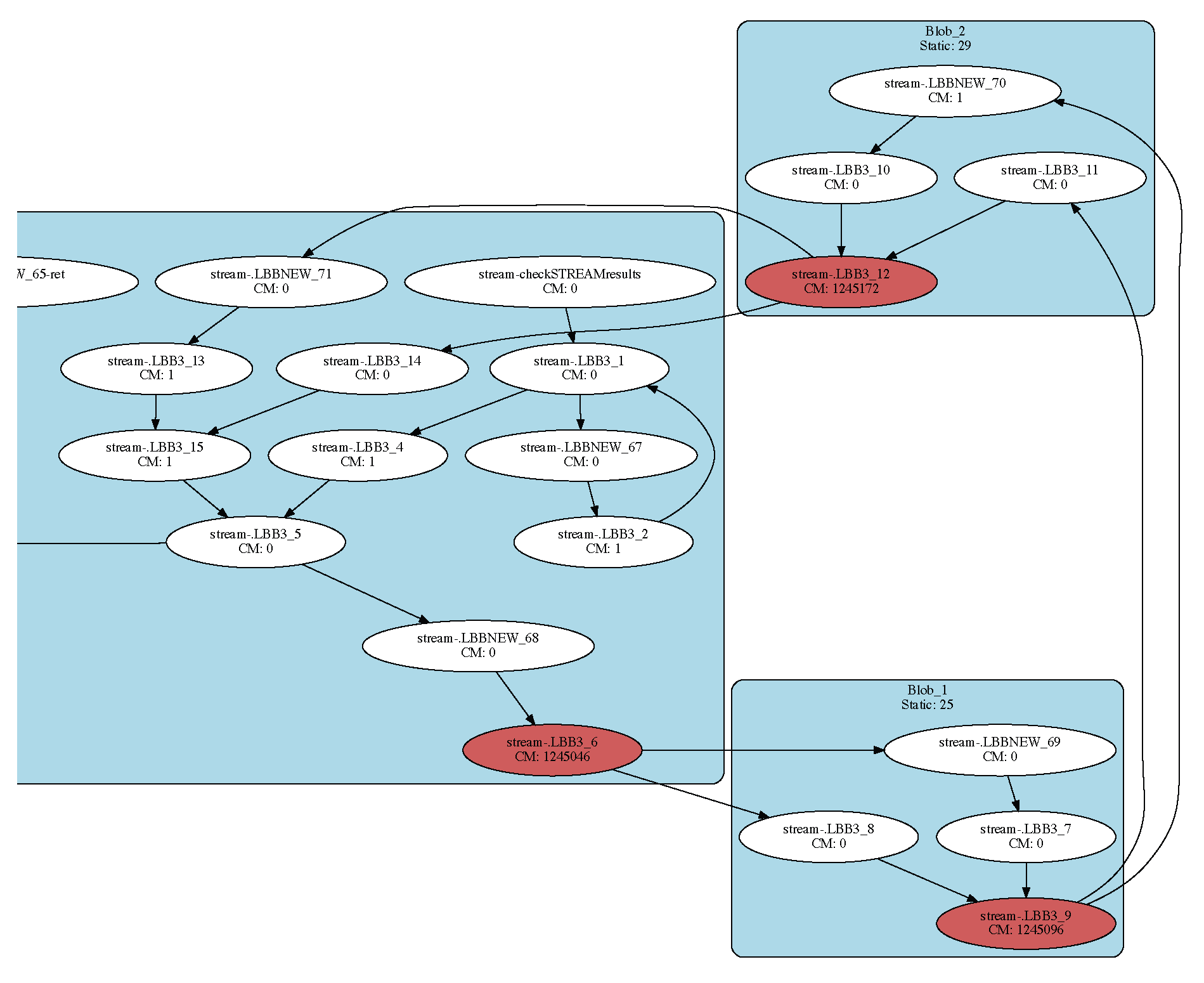
Figure 16.
Machine Learning Model Approach
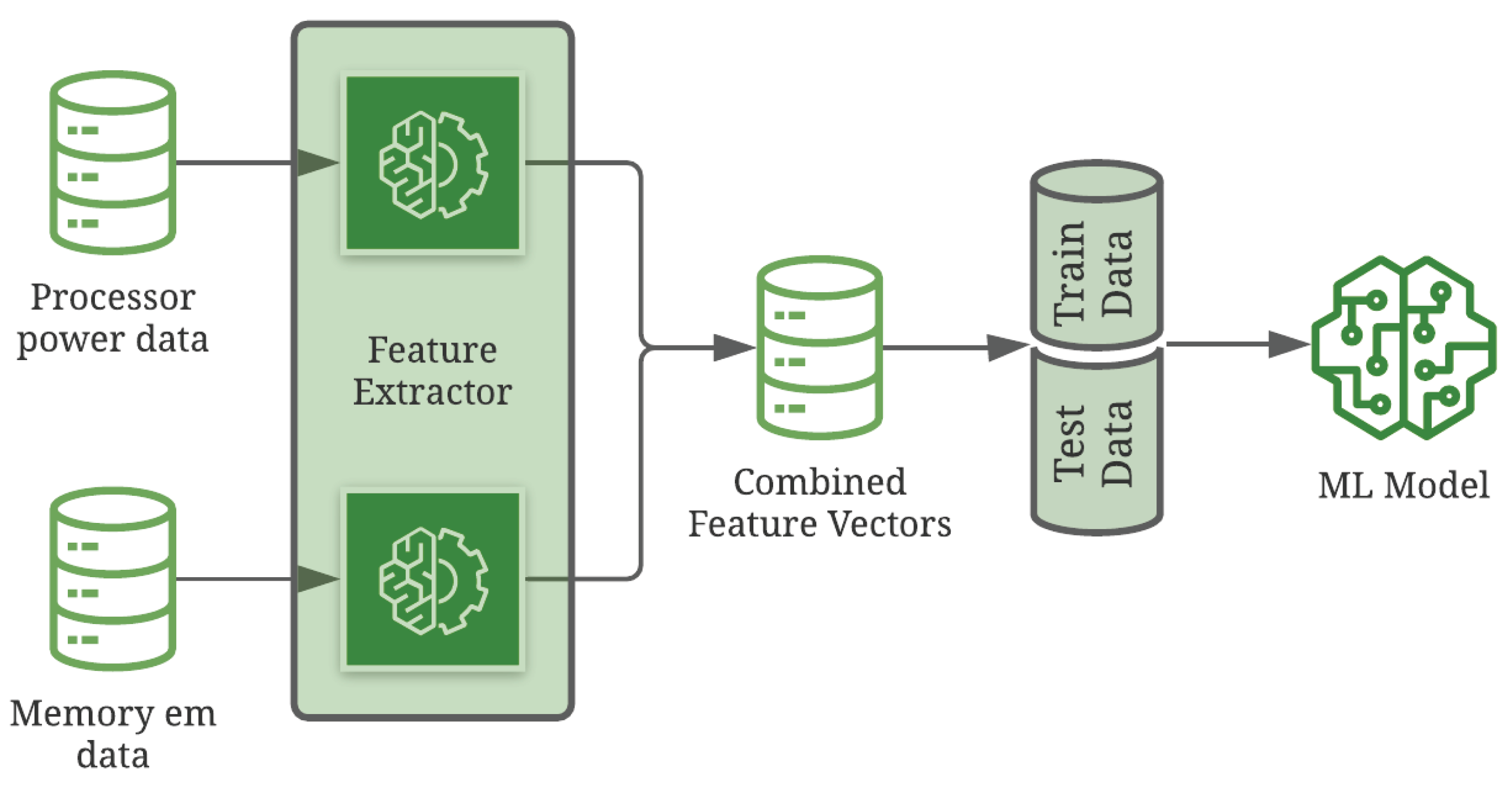
Figure 17.
Path-based Identification data structure
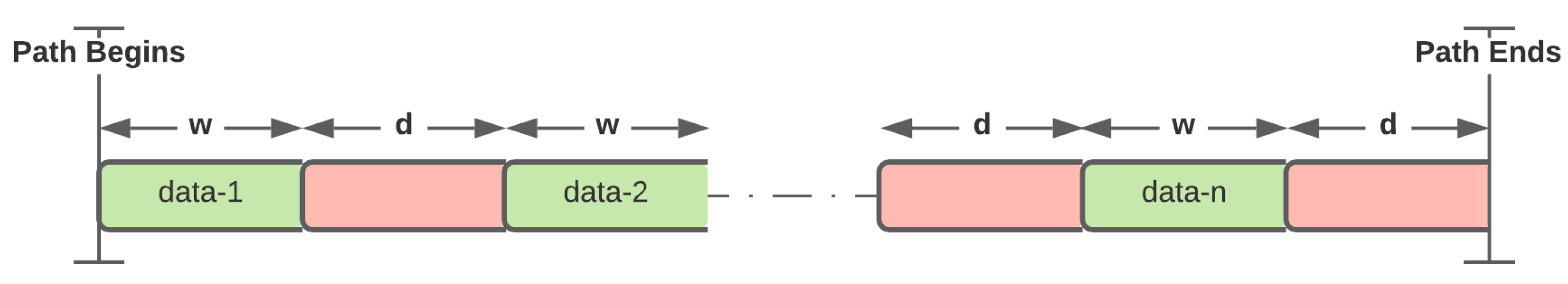
Figure 18.
Token Runs for each class variable
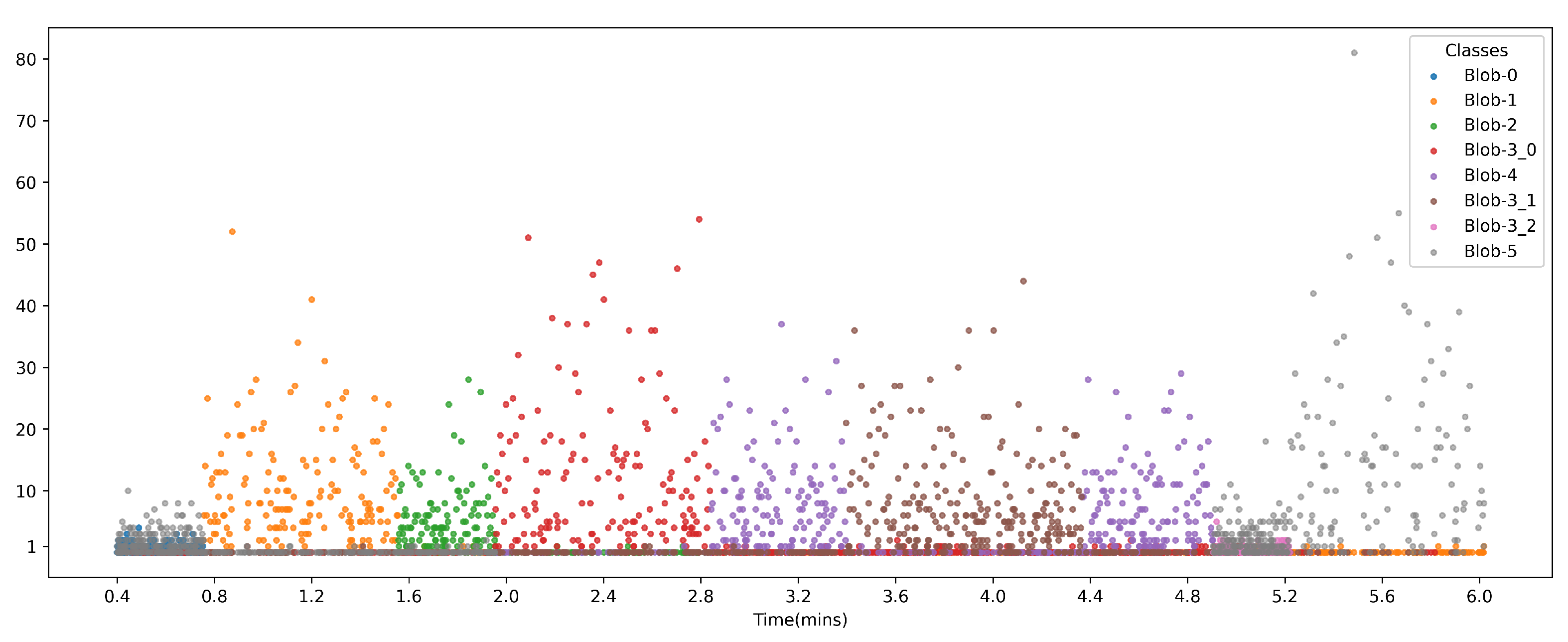
Figure 19.
Blob-based Identification data structure
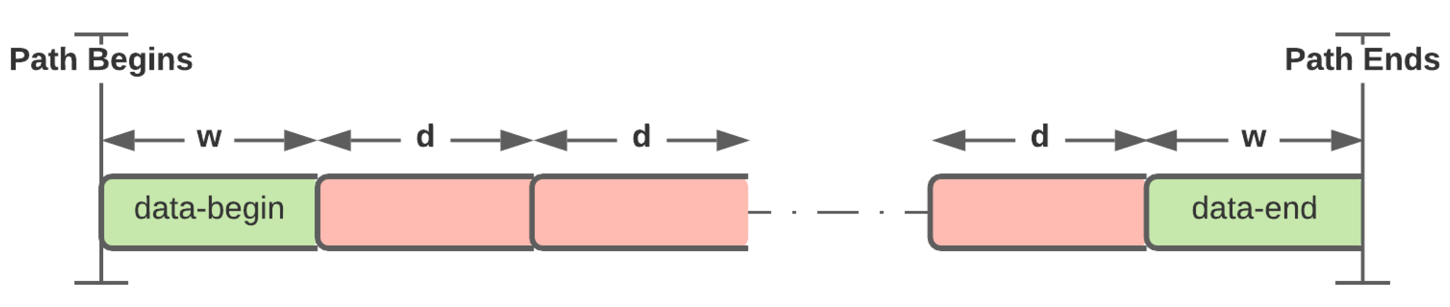
Figure 20.
Confusion Matrix For Address Decision Tree Classifier Model
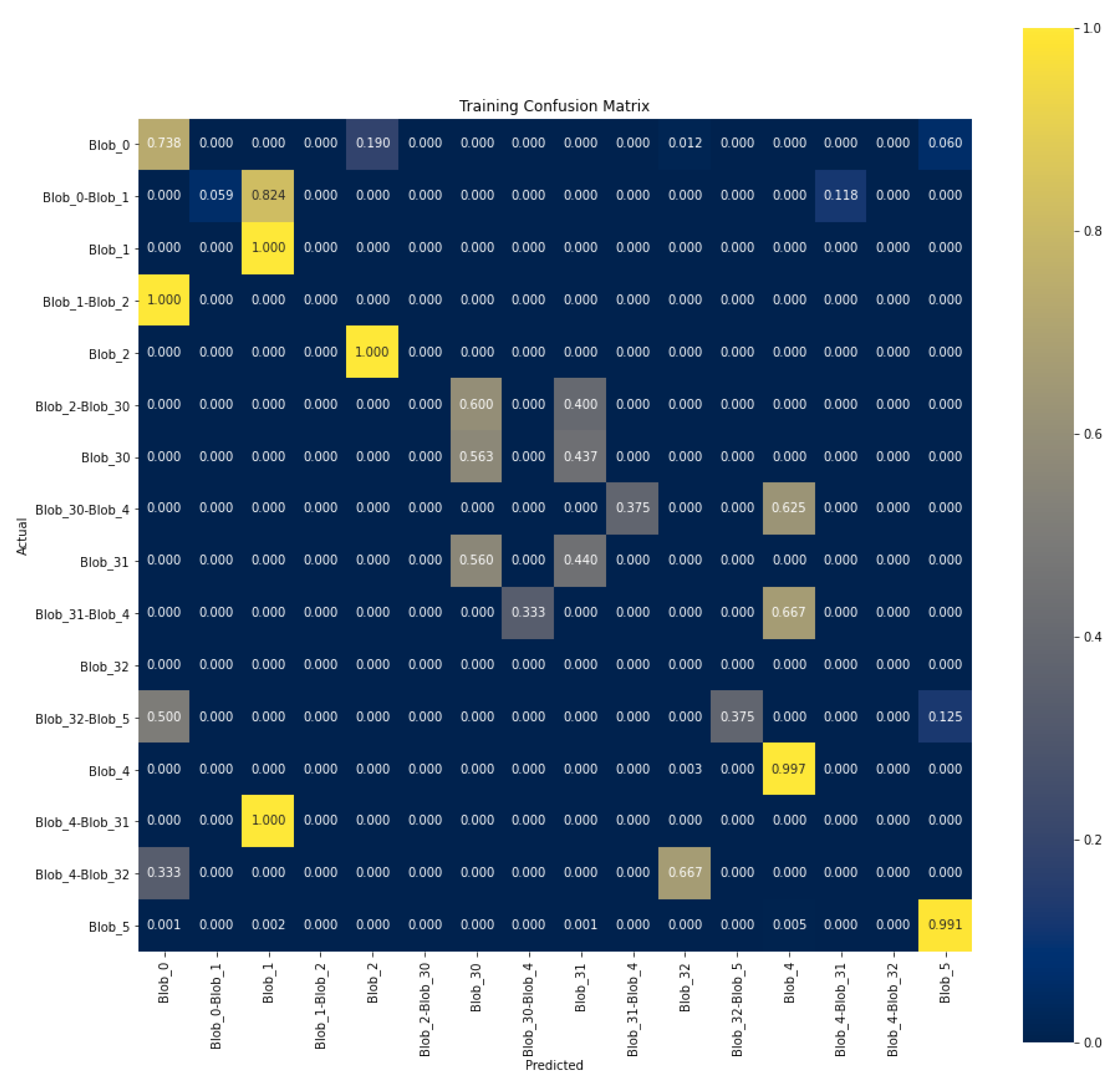
Figure 22.
Results for Blob-level localization (anomaly-free data)
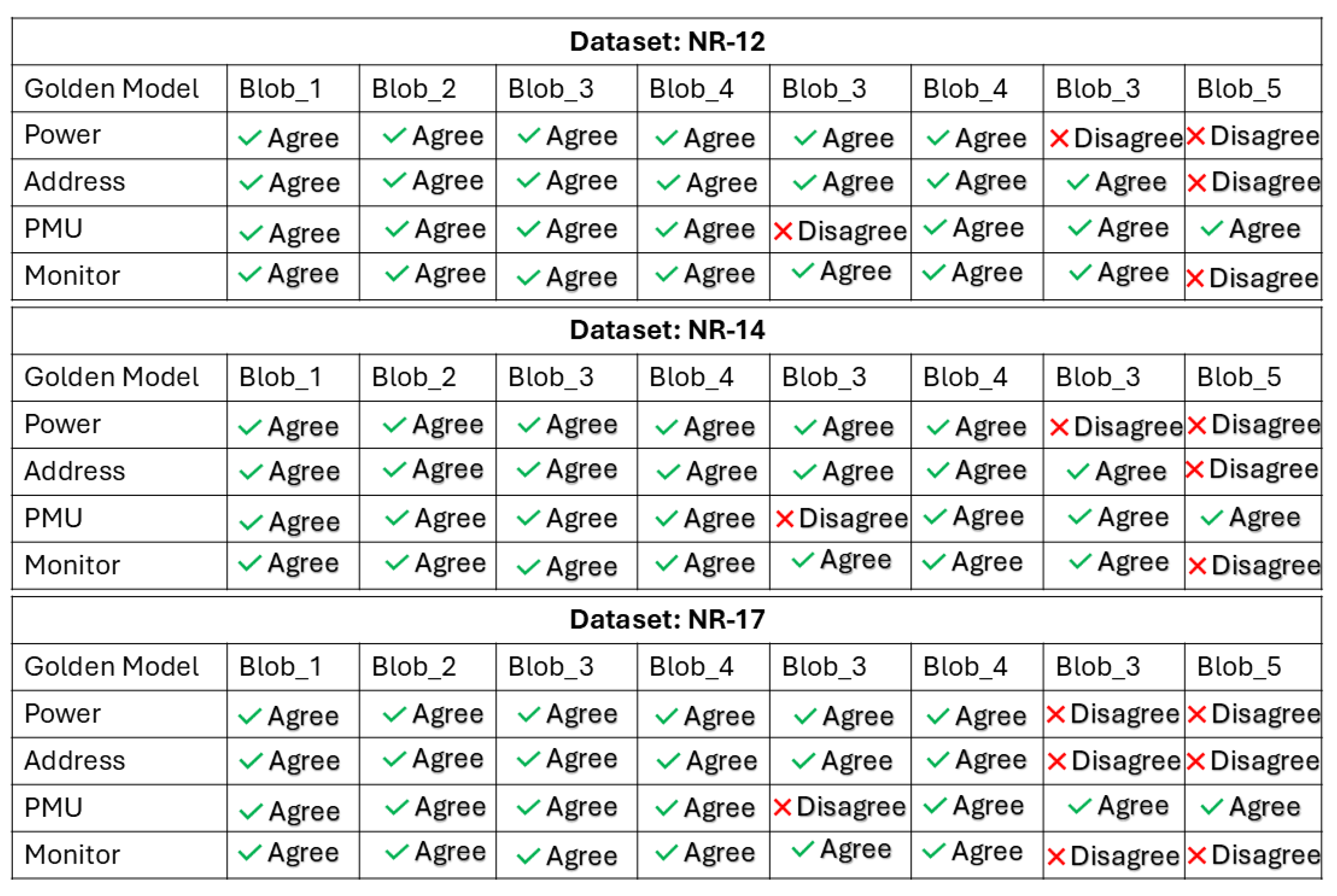
Figure 23.
Results for Path-level localization (anomaly-free data)
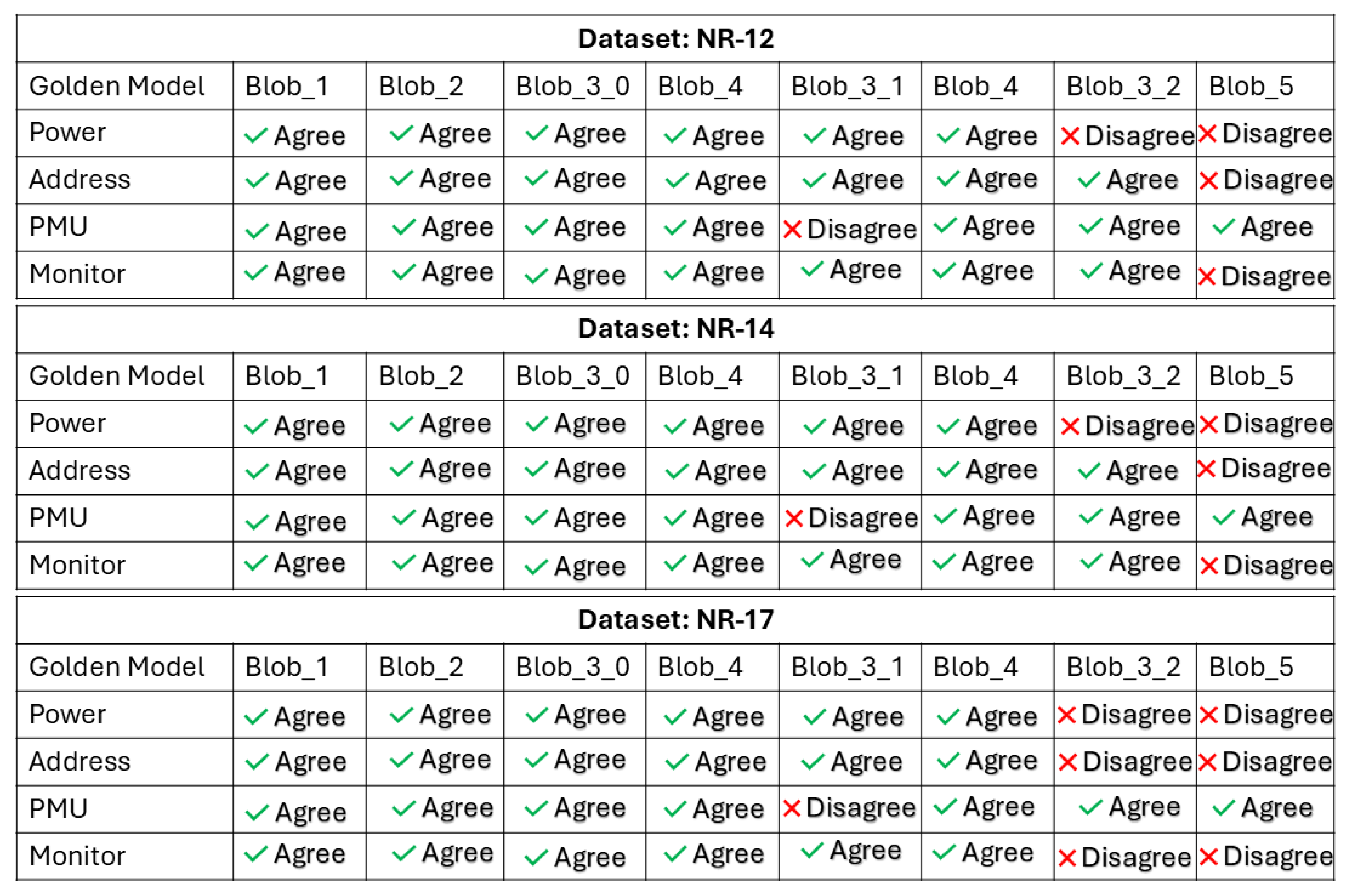
Figure 24.
Results for Blob-level localization (anomalous data)
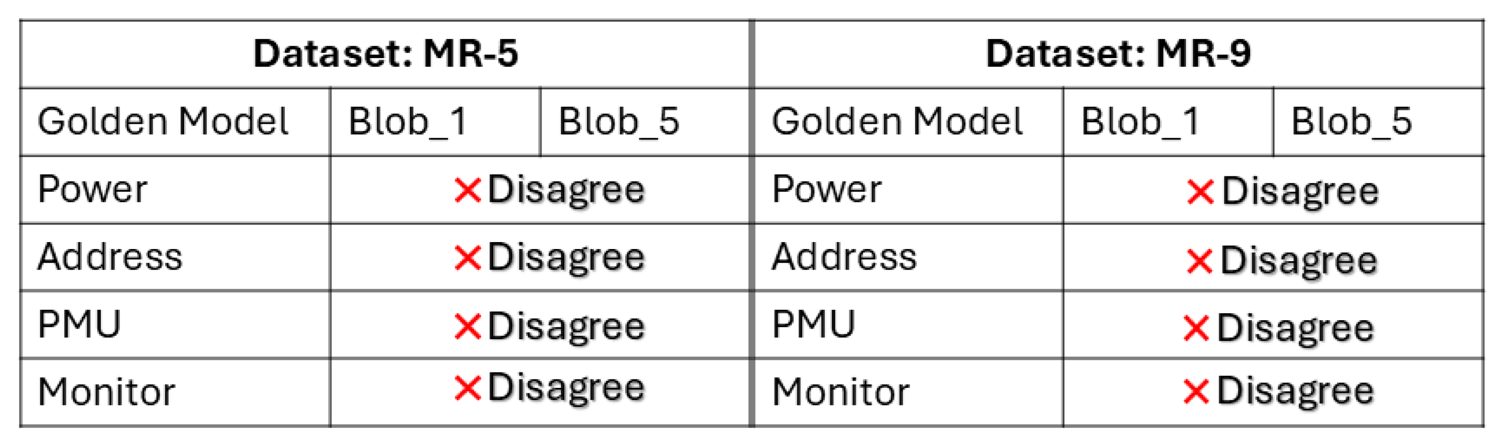
Figure 25.
Results for Path-level localization using majority windows (anomaly-free data)
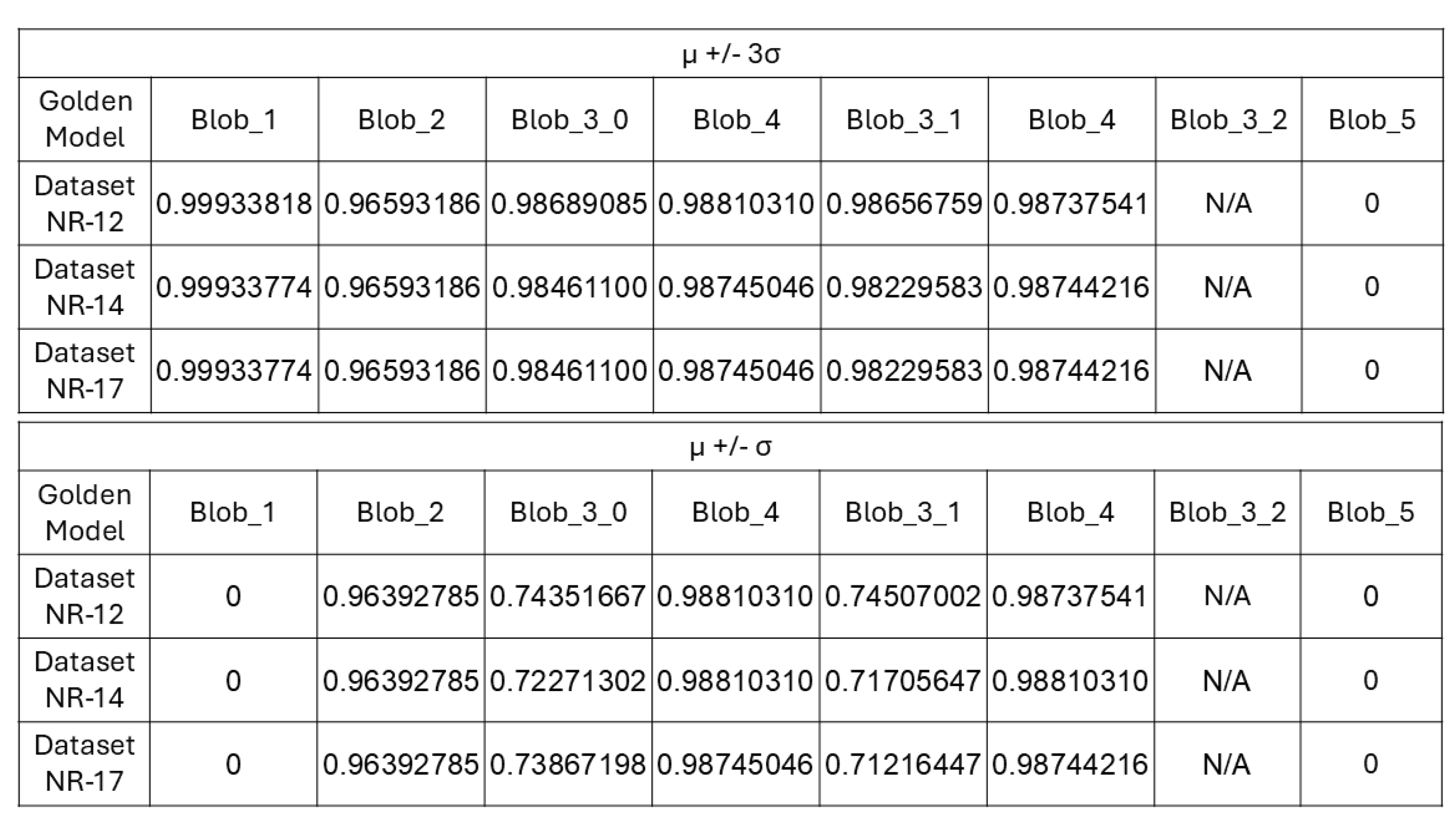
Table 1.
Natural loops approach: average dynamic statistics per blob
| blob | count | Dynamic Instructions | Inst. Before | Inst. After | |||
|---|---|---|---|---|---|---|---|
| mean | min | max | Miss (mean) | Exit (mean) | |||
| 0 | Blob_0 | 1 | 14241 | 14241 | 14241 | 0 | 11 |
| 1 | Blob_1 | 1 | 260400425 | 260400425 | 260400425 | 11 | 343634 |
| 2 | Blob_2 | 1 | 170002890 | 170002890 | 170002890 | 343634 | 6 |
| 3 | Blob_3 | 3 | 400284005 | 31757 | 600410146 | 102497 | 273254 |
| 4 | Blob_4 | 2 | 240153748 | 240000020 | 240307477 | 409879 | 153742 |
| 5 | Blob_5 | 1 | 740003339 | 740003339 | 740003339 | 5 | 0 |
Disclaimer/Publisher’s Note: The statements, opinions and data contained in all publications are solely those of the individual author(s) and contributor(s) and not of MDPI and/or the editor(s). MDPI and/or the editor(s) disclaim responsibility for any injury to people or property resulting from any ideas, methods, instructions or products referred to in the content. |
© 2025 by the authors. Licensee MDPI, Basel, Switzerland. This article is an open access article distributed under the terms and conditions of the Creative Commons Attribution (CC BY) license (http://creativecommons.org/licenses/by/4.0/).
Copyright: This open access article is published under a Creative Commons CC BY 4.0 license, which permit the free download, distribution, and reuse, provided that the author and preprint are cited in any reuse.


