Submitted:
03 December 2025
Posted:
05 December 2025
You are already at the latest version
Abstract
Accurate precipitation prediction is critical for water security and disaster mitigation, yet remains challenging due to atmospheric complexity and class imbalance in rainfall data. This study introduces an integrated "architecture-feature-augmentation" framework to address these limitations. Through systematic comparison of CNN-LSTM and Trans-former architectures, we identify a fundamental trade-off: CNN-LSTM demonstrates higher enhanceability, achieving 80% recall for heavy rainfall when combined with phys-ics-informed augmentation, while Transformer shows superior inherent sensitivity (75% recall) but greater vulnerability to data distribution shifts. Feature engineering benefits are model-specific, significantly improving CNN-LSTM but often introducing redundancy for Transformer. Notably, oversampling techniques like SMOTE achieve peak F1 scores but with substantial generalization gap (ΔF1 > 0.47), indicating overfitting risks, whereas physics-informed augmentation proves more reliable. We establish a principled decision framework: for robust predictions, use CNN-LSTM with physics-informed augmentation; for peak performance where risks are tolerable, employ CNN-LSTM with SMOTE. These findings provide scientific guidance for extreme weather preparedness and water resource management.
Keywords:
deep learning
; class imbalance
; data augmentation methods
; feature engineering
; time series forecasting
1. Introduction
Accurate precipitation prediction is critical for water resource management, agricultural planning, and disaster early warning systems, a importance further elevated by the increasing frequency of extreme events under climate change [1,2,3,4,5,6,7,8,9,10,11,12]. However, achieving high-accuracy prediction remains a formidable challenge due to the complex, nonlinear, and non-stationary nature of precipitation mechanisms [13,14,15,16].
The methodology for precipitation prediction has evolved from statistical models to machine learning (ML) and recently to deep learning techniques [17]. Early statistical approaches like ARIMA established a foundation for linear time-series forecasting but struggled with nonlinear dynamics and integrating multi-source meteorological variables [18,19,20]. Subsequent ML methods, including Support Vector Machines (SVM) and Random Forests (RF), offered powerful nonlinear fitting capabilities [21,22,23,24,25,26,27]. For instance, Tang et al. (2022) demonstrated that data augmentation methods like SMOTE could significantly boost the performance of shallow models like XGBoost [28]. Nonetheless, these models rely heavily on manual feature engineering and their inherent structures (e.g., tree-based architectures) are limited in capturing raw spatiotemporal dependencies [26].
Deep learning has since brought transformative progress. Architectures such as CNNs enabled automatic spatial feature extraction, while the Convolutional LSTM (ConvLSTM) integrated CNNs with LSTMs, establishing a milestone for spatiotemporal sequence forecasting [29,30]. More recently, the Transformer architecture has emerged as a prominent focus due to its powerful global dependency modeling, leading to advanced frameworks like PrecipNet, SwinNowcast, and TransMambaCNN for tasks including downscaling, nowcasting, and extreme event prediction [31,32,33,34].
Despite these advances, deep learning—being inherently data-intensive—faces significant challenges under extreme class imbalance, where critical heavy rainfall events may constitute only a small fraction of samples [35]. In such scenarios, models exhibit a pronounced bias toward the majority class, failing to predict rare extremes. While data augmentation is a potential solution, its application in hydrology remains exploratory and often lacks physical consistency constraints [35]. Moreover, augmentation techniques like SMOTE yield markedly lower performance gains in deep learning models (e.g., LSTM) compared to their substantial benefits in shallow ML, a limitation likely more pronounced in parameter-rich architectures like Transformer [28]. Consequently, effectively addressing class imbalance under data-scarce and physically constrained conditions remains a core bottleneck.
In summary, a critical research gap exists at the intersection of deep learning and daily-scale extreme precipitation prediction, constrained by limited samples and extreme class imbalance. Existing work primarily focuses on architectural refinements, with insufficient systematic investigation into the synergistic effects between data augmentation strategies and deep learning architectures [36]. Developing augmentation frameworks that incorporate physical constraints to ensure data realism is particularly crucial.
To address these challenges, this study constructs a comprehensive synergistic decision-making framework integrating "Architecture-Feature-Augmentation" for the Yongcui River Basin. Our key contributions are:
- Development of a spatiotemporal integrated meteorological feature set, incorporating lag processing, rolling window statistics, and physically coupled features, refined via Random Forest for enhanced interpretability.
- Systematic evaluation of architecture-augmentation synergy, comprehensively assessing multiple strategies under extreme imbalance conditions.
- Design of physics-constrained data augmentation, enforcing meteorological evolution laws to ensure physical plausibility.
- Establishment of a multi-dimensional evaluation system, including Recall and F1-score, to thoroughly assess minority class identification and stability.
2. Materials and Methods
2.1. Study Area
This study is conducted in the Yongcui River Basin, a typical high-latitude forest ecosystem located in the Lesser Khingan Mountains of Heilongjiang Province, China (Figure 1). The basin drains an area of approximately 703 km² and is characterized by high vegetation coverage with minimal human disturbance.
The region experiences a cold-temperate continental monsoon climate, with an average annual precipitation of 650–800 mm that is highly unevenly distributed (Figure 2) [37]. Over 70% of the annual precipitation occurs from June to September, with heavy rainfall events predominantly concentrated in July and August. This temporal concentration, combined with the complex terrain, results in a precipitation dataset with marked seasonal imbalance and a zero-inflated long-tail distribution. These inherent data characteristics make the basin an exemplary case for evaluating deep learning models under extreme class imbalance and sample scarcity.
2.2. Materials
This study utilized daily meteorological and precipitation data from 1980 to 1999 for the Yongcui River Basin. Meteorological variables, including temperature (mean, max, min), pressure, relative humidity, wind speed, and sunshine duration, were sourced from the Yichun National Reference Climatological Station. Daily precipitation data were obtained from the Heilongjiang Hydrological Yearbook. The high-quality 20-year series (7,300 samples) underwent linear interpolation for minimal missing values.
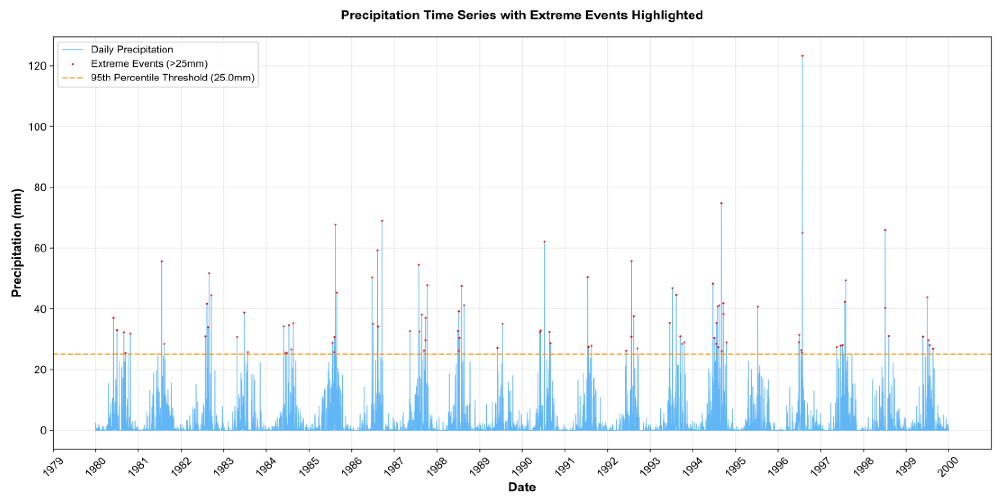
The precipitation data exhibit a pronounced "zero-inflated" and right-skewed distribution (Figure 2). Events were classified into three categories: no rain (0 mm), general precipitation (0.1–24.9 mm), and heavy rainfall (≥25 mm). A 25 mm threshold was adopted instead of the common 50 mm standard to better identify hydrologically significant events in this region (Figure 4).
A systematic feature engineering pipeline was implemented, encompassing raw data preprocessing, temporal feature construction, and the design of physically coupled features, followed by feature selection to enhance model performance.
Critically, the dataset exhibits severe class imbalance (Figure 3) [39]. The training set contains only 81 heavy rainfall samples (vs. 3,610 no-rain and 2,063 general precipitation), and the test set merely 20 (vs. 934 and 507). This scarcity of heavy rainfall events substantially impedes model training, leading to low F1-scores and posing a core challenge for accurate identification of these critical events [38].
Figure 3.
Class distribution comparison of precipitation datasets:(a) training set (before augmentation),(b) training set (after augmentation) and (c) test set.
Figure 3.
Class distribution comparison of precipitation datasets:(a) training set (before augmentation),(b) training set (after augmentation) and (c) test set.
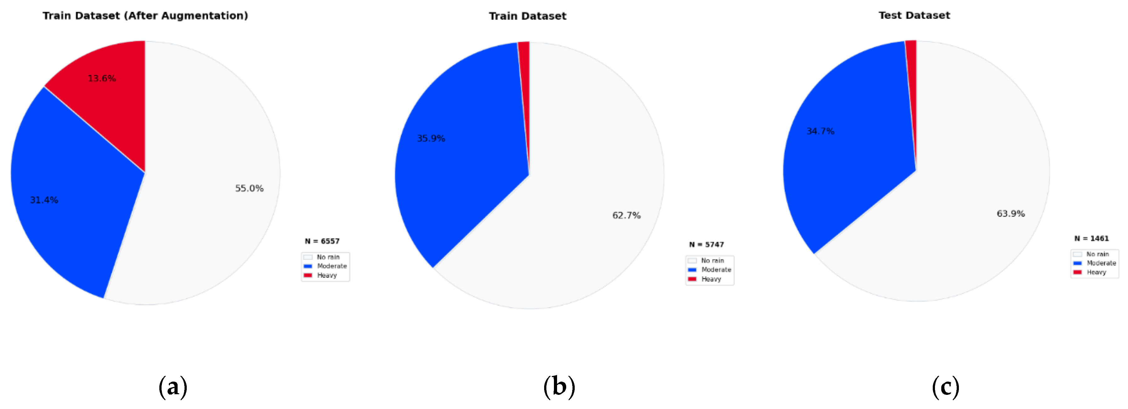
Figure 4.
Daily precipitation time series with extreme events highlighted.
3. Methods
3.1. Feature Selection
To mitigate the risks of dimensionality inflation and overfitting caused by redundant features, this study established a three-tier feature selection pipeline[40]。
- 1.
- Standardization:The feature matrix X ∈ R^(n×d) was standardized using Z-score normalization, calculated as follows:In this equation, μj and σj represent the mean and standard deviation of the j-th feature.
- 1.
- Redundant Feature Elimination: Features exhibiting high linear correlation (∣r∣>0.8) were removed, and low-variance features (σ 2<0.01) were filtered out. This step aimed to reduce inter-feature redundancy and enhance feature independence.
- 2.
- Feature Selection: Based on the feature importance ranking derived from the Random Forest algorithm (see Figure 2), the top 30 most discriminative features were selected. This method evaluates the average contribution of a feature during node splits in the tree models, thereby measuring its impact on the classification outcome [41,42].
The importance score for a feature f, denoted as I(f), quantifies its contribution to the model's decision-making process, typically using Gini importance or mean decrease in impurity. This pipeline effectively improved the utilization efficiency of the feature space, reduced the adverse impact of redundant information on model performance, and simultaneously enhanced the model's interpretability.Figure 5 presents the feature importance rankings derived from the binary and ternary classification models.
Figure 5.
Feature importance ranking for three-class heavy rainfall prediction.
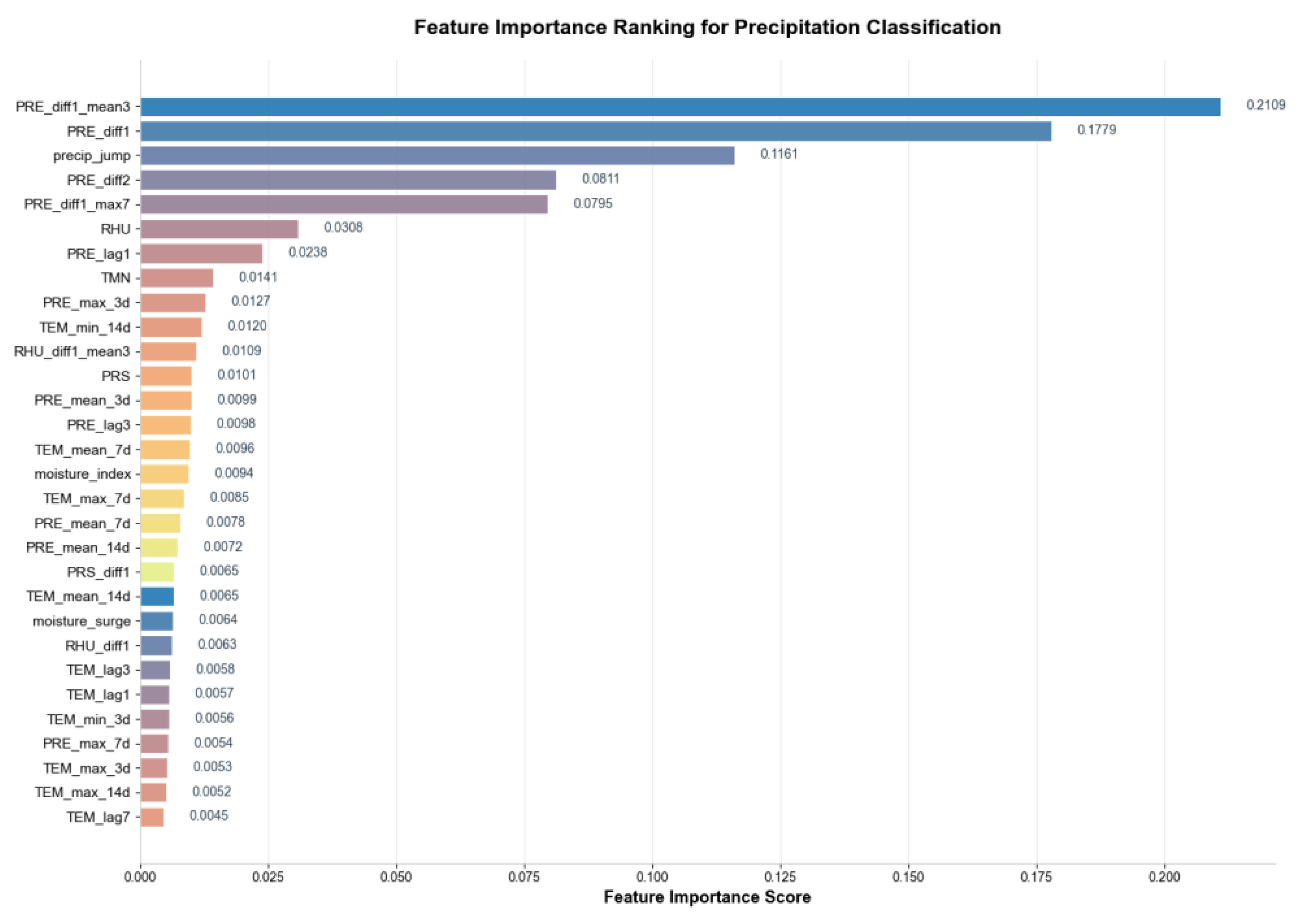
Figure 6.
Feature importance ranking for two-class heavy rainfall prediction.
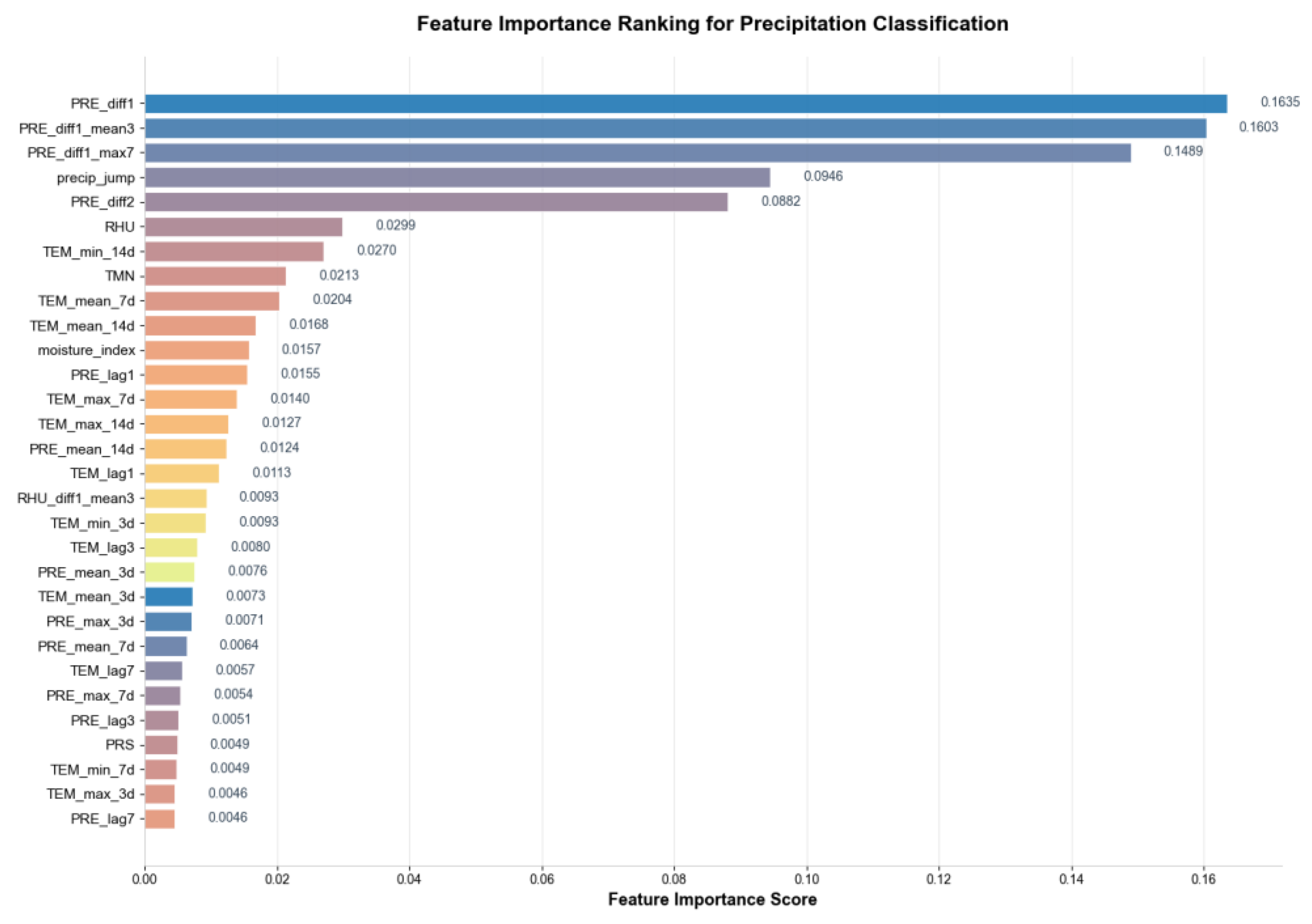
The final selection of the top 30 features by importance ranking achieved a cumulative contribution rate of 85.3%. Precipitation variation features (e.g., PRE_diff1_mean3, PRE_diff1, etc.) were dominant, demonstrating consistency with the abruptness characteristic of heavy rainfall events.
3.2. Sample Ugmentation Strategy
The extreme class imbalance, with heavy rainfall samples constituting only 1.4% of the dataset, biases deep learning models toward the majority class, severely limiting their ability to identify critical precipitation events [39]. To mitigate this, we implemented and evaluated four distinct augmentation strategies, categorized into interpolation-based and generative approaches, to systematically explore the synergy between data augmentation and model architecture.
Interpolation-based Oversampling: SMOTE-TS and ADASYN.
We employed two variants of the Synthetic Minority Over-sampling Technique (SMOTE) designed for time-series data. The SMOTE-TS algorithm generates synthetic samples via linear interpolation between temporally adjacent minority class instances [43,44]:
Building on this, the Adaptive Synthetic Sampling (ADASYN) algorithm incorporates an adaptive mechanism to preferentially generate samples near the feature space boundaries of difficult-to-learn minority instances [46,47,48]. While both methods effectively increase minority sample size, they do not explicitly enforce physical consistency among the generated meteorological variables, potentially introducing implausible data points [45].
Physics-Constrained Perturbation Augmentation
To address the physical inconsistency limitation of interpolation methods, we developed a novel physics-constrained perturbation strategy [49,50]. This method applies controlled random perturbations (±5%) to temperature and relative humidity of existing heavy rainfall samples. Crucially, it enforces a monotonic pressure decrease constraint (PRS(t+1) < PRS(t)) to maintain physical consistency with atmospheric instability mechanisms preceding heavy rainfall. This approach enhances model robustness while ensuring the augmented data remains physically plausible.
Generative Adversarial Network (TimeGAN & Light-TimeGAN).
TAs a generative alternative, we implemented a Time-Series Generative Adversarial Network (TimeGAN) and its lightweight variant (Light-TimeGAN) to capture underlying temporal distributions [51,52,53]. The Light-TimeGAN architecture employs single-layer LSTM networks for both generator and discriminator, trained on all available heavy rainfall samples (N=81) using the Adam optimizer. To ensure meteorological plausibility, we integrated verification mechanisms including variable range validation, metadata inheritance, and statistical feature constraints via a feature matching loss. These mechanisms enhance the physical realism and stability of the generated sequences.
All augmentation strategies were implemented through a unified Python framework. The heavy rainfall augmentation factor was controlled by the parameter heavy_rain_aug_factor (set to 10) to ensure consistent and comparable experimental conditions across all models.
3.3. Data Partitioning Strategy
To prevent data leakage and preserve temporal coherence, we partitioned the 20-year dataset (1980–1999) using an annual stratified time series split. This approach ensures that the model is trained on past data and evaluated on future data, maintaining a realistic forecasting scenario and providing a robust assessment of generalization capability [57,58,59]. A three-fold validation scheme was employed, with each fold containing non-overlapping blocks of years for training and validation, thus eliminating cross-year boundary leakage. Table 1 depicts the specific temporal distribution of the three-fold splits.
3.4. Evaluation Metrics
A multi-tiered evaluation framework was adopted to rigorously assess model performance, with a primary focus on the detection of rare heavy rainfall events. The selected metrics are as follows:
Overall Performance: Accuracy and the Area Under the ROC Curve (AUC-ROC) were used to evaluate general discriminative capability.
Heavy Rainfall Detection: Recall and F1-score for the heavy rainfall class served as the primary metrics to quantify the model's sensitivity and precision in identifying critical events.
Imbalance Adjustment: Balanced Accuracy was incorporated to mitigate interpretive biases caused by class imbalance.
This framework ensures a comprehensive assessment aligned with the operational priority of maximizing extreme weather event detection.
3.5. Threshold Decision Mechanism
To enhance the stability and generalization of the classification threshold, we implemented a three-fold averaging methodology. The final decision threshold (τ) was set as the arithmetic mean of the three optimal thresholds, each identified as the point maximizing the F1-score for the heavy rainfall category within a validation fold:
This strategy mitigates threshold fluctuations caused by data partitioning randomness, thereby enhancing predictive robustness.
3.6. Monsoon Feature Enhancer
The month variable (m ∈ [1,12]) was processed through an Enhanced Monsoon Embedder to capture seasonal climate patterns. To avoid imposing ordinal bias, we first applied a discrete sinusoidal embedding. This was subsequently transformed by a two-layer nonlinear network into a optimized 64-dimensional representation:
The resulting temporal embedding e_month was then concatenated with the CNN-encoded meteorological features, followed by unified normalization. This design enables seasonally adaptive feature weighting, enhancing the model's capacity to capture regional precipitation regimes through dynamically modulated representations.
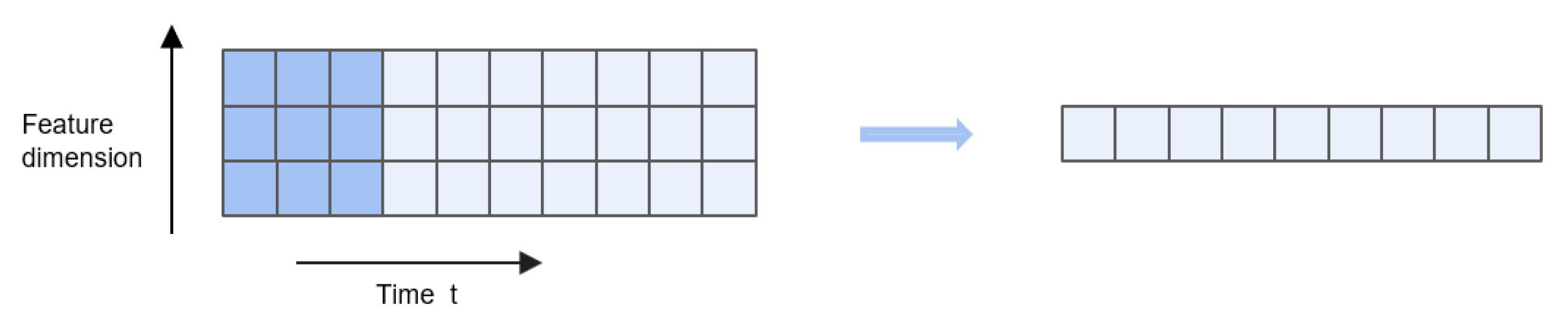
3.7. Input Windowing Strategy
To capture medium-term and long-term dependencies in precipitation patterns, this study constructs input samples using a sliding time window approach. Each sample consists of consecutive meteorological observations from the preceding 90 days, with the objective of predicting the precipitation category of the target day (day 91). The 90-day window length was empirically determined to be optimal through validation set performance, effectively balancing the coverage of characteristic seasonal variation cycles against potential noise introduction and computational burden associated with longer sequences.
4. Model Architecture
4.11. D-CNN
Convolutional Neural Networks (CNNs) form a foundational deep learning architecture. While their two-dimensional (2D-CNN) and three-dimensional (3D-CNN) variants are commonly employed in image and video recognition, one-dimensional convolutional networks (1D-CNN) are particularly suited for time series analysis. This study utilizes a 1D-CNN to model local temporal characteristics within meteorological sequences, with a focus on capturing short-term fluctuation patterns in variables such as temperature, humidity, and atmospheric pressure preceding heavy rainfall events. The input data is structured as sequential tensors with dimensions (B, T, F), representing batch size, time steps, and feature dimension, respectively[62]。Initially, input features are projected into a 64-dimensional latent space through linear transformation to standardize feature scales and enhance representation capacity:
h_t = ReLU(W_proj x_t + b)
The temporal embedding vector is then concatenated with the transformed features to create an enhanced feature representation: . This composite feature is subsequently processed through convolutional layers (kernel size=3, stride=1), batch normalization, and ReLU activation, followed by max-pooling operations (window size=2) to extract abstract representations of local temporal patterns. These processing steps systematically compress the temporal dimension from T to T/2, effectively smoothing high-frequency noise while amplifying subtle pressure fluctuation signals that typically precede rainfall events. The resulting refined features provide optimized inputs for subsequent temporal dependency modeling stages. Figure 7 illustrates the architecture of a one-dimensional convolutional neural network (1D CNN).
Figure 7.
1D-CNN with a single convolution kernel with a size of 3×3.
4.2. BiLSTM
Long Short-Term Memory (LSTM) networks effectively capture dynamic temporal dependencies through specialized gating mechanisms, overcoming the vanishing and exploding gradient problems associated with traditional recurrent neural networks. However, conventional LSTMs process sequences solely in the forward temporal direction, unable to leverage potentially informative reverse dependencies[15]。
Bidirectional LSTM (BiLSTM) architectures address this limitation by incorporating both forward and backward processing units, enabling simultaneous modeling of temporal dependencies in both directions. The implemented network employs hidden layers with 128 units, substantially enhancing its capacity for comprehensive temporal feature representation.The update process can be formally expressed as:
The final output is obtained by concatenating the hidden state vectors from both directions:
This architecture facilitates bidirectional feature propagation across the entire temporal sequence, significantly enhancing the model's capacity to represent the dynamic evolution patterns characteristic of heavy rainfall events. Through BiLSTM's dual-directional modeling mechanism, the framework concurrently captures both gradual seasonal precipitation trends and abrupt heavy rainfall signals, thereby establishing a robust foundation for comprehensive temporal dependency modeling within the prediction system.
4.31. DCNN-BILSTM
This study develops a CNN-BiLSTM hybrid model that synergistically combines 1D-CNNs for local pattern extraction with bidirectional LSTM networks for capturing long-range, bidirectional temporal dependencies. The model processes input sequences of dimensions (N, T, D) as follows.
First, raw meteorological features are enhanced by concatenation with 16-dimensional seasonal embeddings generated from an Enhanced Monsoon Embedder. The composite sequence is then fed into a 1D-CNN module to extract salient short-term fluctuation patterns and compress the temporal dimension. The resulting local features are subsequently processed by a two-layer bidirectional LSTM (256 hidden units per layer) to model the long-range evolution of precipitation systems. Finally, the output from the last temporal step is passed through fully connected layers to generate probability distributions over the precipitation categories. To mitigate class imbalance, the model is trained using Focal Loss, with optimization details provided in Section 4.5. The model architecture diagram is shown in Figure 8.
4.4. Improved Transformer
While the standard Transformer excels in global dependency modeling via multi-head self-attention, its application to non-stationary meteorological sequences often results in over-smoothed representations and diminished sensitivity to critical local variations [63]. To address this, we introduce an improved Precipitation Transformer.
Our architecture adapts the standard Transformer [63] for precipitation classification through three key modifications: (1) the decoder is removed as the task requires classification, not generation; (2) a seasonal embedding module is incorporated to enhance temporal awareness of monthly variations; and (3) an attention-based learnable pooling mechanism replaces standard pooling, using trainable query vectors to generate a globally contextualized representation via weighted feature aggregation. These enhancements collectively enable the model to more effectively capture the complex, evolving patterns in meteorological data. Figure 9 presents the model architecture diagram.
4.5. Raining Configuration
To address the extreme class imbalance, we employed Focal Loss (α=0.25, γ=2) as the training objective, which dynamically scales the cross-entropy loss to focus learning on hard, minority-class examples. All models were optimized using Adam with a consistent learning rate of 1×10⁻³. Training incorporated early stopping to prevent overfitting. Detailed hyperparameters (e.g., scheduler, batch size) are provided in Appendix A. This unified setup ensures fair comparability across all architectural and augmentation experiments.
5. Results and Discussion
5.1. The Impact of Data Augmentation Methods on Model Performanc
5.1.1. Comparison of Data Augmentation under Three-Class Classification Task
The efficacy of data augmentation strategies for the three-class precipitation task varied significantly between CNN-LSTM and Transformer models, highlighting a strong dependence on base architecture (Table 2).
For CNN-LSTM, SMOTE yielded the most balanced improvement, elevating the macro-F1 score to -0.0187 from a baseline of -0.0241. It achieved the highest F1-scores for both no-rain (0.6482) and general-rain (0.5023) categories, along with the highest AUC (0.6578) and balanced accuracy (0.7233) among all configurations. Its expected calibration error (ECE=0.0661) remained low, confirming that these gains were achieved without compromising predictive reliability. In contrast, the GAN-based method substantially improved heavy rainfall recall to 0.2488 (from 0.15), but this came at the cost of a higher ECE (0.0859) and lower balanced accuracy (0.5198), indicating enhanced minority-class sensitivity at the expense of increased predictive uncertainty.
The Transformer model exhibited more complex and unstable responses to data augmentation. Without augmentation, it achieved an exceptionally high heavy rainfall recall (0.75), but severely compromised general-rain recognition (F1-score: 0.3477), resulting in a net performance regression (ΔF1 = -0.0373) and a substantially elevated ECE (0.1032), indicating poor calibration. Even with SMOTE, the Transformer's overall performance degraded (ΔF1 = -0.0476, AUC = 0.5978), and its moderate balanced accuracy (0.6677) and ECE (0.0655) could not compensate for this core performance regression. The performance metrics for the eight experimental trials of the binary classification task are presented in Table 2.
5.1.2. Comparison of Data Augmentation under Binary Classification Task
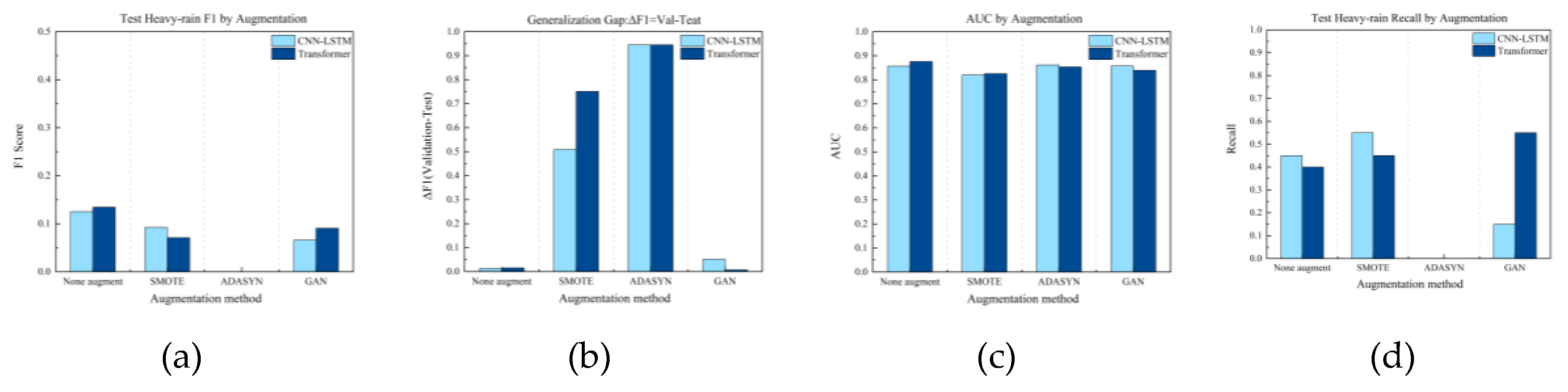
For the binary classification task (heavy rain vs. non-heavy rain), data augmentation strategies—particularly oversampling—failed to produce stable gains and generally amplified overfitting, demonstrating limited utility after category simplification.
As shown in Table 3, the unaugmented baselines achieved test F1-scores of 0.1250 (CNN-LSTM) and 0.1345 (Transformer) for the "rain" class, substantially outperforming most augmented configurations, while their lower expected calibration errors (ECEs of 0.4145 and 0.3556, respectively) indicated better-calibrated predictions. In contrast, oversampling techniques like SMOTE and ADASYN induced significant degradation; for instance, ADASYN nearly zeroed the Transformer's "rain" F1-score, indicating severe instability. These methods also elevated ECE values (e.g., 0.4382 for CNN-LSTM+SMOTE), confirming poor calibration. Furthermore, the generalization gap (ΔF1) for SMOTE and ADASYN reached 0.50-0.95, drastically exceeding the baseline (~0.01), which confirms severe overfitting due to inflated validation performance. While the GAN-based method showed marginal benefits in isolated cases (e.g., a lower ECE of 0.3527 for Transformer), its overall effectiveness was unstable and failed to consistently surpass the baseline, as evidenced by its low F1-score (0.0905) and limited comprehensive benefit.
In conclusion, for binary precipitation detection, data augmentation—especially oversampling—did not improve generalization and likely introduced feature redundancy and noise, increasing overfitting risk due to the already relatively balanced sample distribution. Architectural selection should therefore be guided by application requirements, with the Transformer offering higher recall potential and the CNN-LSTM providing greater stability. The corresponding results for the ternary classification task are summarized in Table 3.
5.2. Performance Comparison between Model Architectures and Task Types
5.2.1. Comparison of Model Architectures under Three-Class Classification Task
A comparative analysis of the CNN-LSTM and Transformer models for the three-class precipitation task reveals a distinct performance trade-off. The Transformer exhibited a significant and stable advantage in heavy rainfall recall (0.75 vs. 0.15 for CNN-LSTM under unaugmented conditions), showcasing its superior capacity for identifying minority class events. However, this came at the cost of higher predictive uncertainty, as indicated by its elevated expected calibration error (ECE=0.1032 vs. 0.0644).
Conversely, the CNN-LSTM demonstrated greater overall stability and generalization, achieving a marginally higher heavy rainfall F1-score (0.1053 vs. 0.0870) and AUC (0.6412 vs. 0.6289). This model also showed higher enhanceability and robustness under data augmentation. With SMOTE, its heavy rainfall recall improved significantly without compromising AUC, indicating effective assimilation of synthetic samples. In contrast, the Transformer's inherent recall advantage diminished with oversampling methods like SMOTE and ADASYN. Notably, while ADASYN yielded the lowest ECE (0.0587) for the Transformer, it concurrently led to a complete failure in heavy rainfall identification, underscoring a fundamental incompatibility.
In summary, architecture selection is objective-dependent. The unaugmented Transformer is preferable for applications prioritizing maximum heavy rainfall recall and tolerating higher calibration error. For scenarios demanding overall discriminative capability, output stability, and predictive reliability, the CNN-LSTM augmented with SMOTE offers a more robust solution. These findings emphasize the necessity of tailoring model configuration to specific operational requirements.
Figure 10.
Comparison of Performance between CNN-LSTM and Transformer Models under Different Data Augmentation Methods for Three-Class Heavy Rainfall Prediction).
Figure 10.
Comparison of Performance between CNN-LSTM and Transformer Models under Different Data Augmentation Methods for Three-Class Heavy Rainfall Prediction).

5.2.2. Comparison of Model Architectures under Binary Classification Task
In the binary precipitation task, with only 20 heavy rainfall instances in the test set, the CNN-LSTM and Transformer architectures exhibited a clear performance trade-off, centered on the prioritization of heavy rainfall recall versus overall discriminative capability and calibration.
The CNN-LSTM demonstrated superior sensitivity to the minority class, achieving a higher heavy rainfall recall (0.45) compared to the Transformer (0.40) under unaugmented conditions. Conversely, the Transformer attained a marginally higher AUC (0.8755) and a lower Expected Calibration Error (ECE=0.3556 vs. 0.4145), indicating stronger global discriminative performance and more reliable probability estimates.
Data augmentation further accentuated their robustness differences. The CNN-LSTM maintained stability, with its heavy rainfall recall improving under SMOTE augmentation, albeit at the cost of a higher ECE (0.4382). In stark contrast, the Transformer exhibited significant fragility, with its performance collapsing under oversampling methods like ADASYN, which resulted in a complete failure in heavy rainfall identification and an anomalously low ECE—an artifact of catastrophic model failure.
For applications where detecting rare extreme events is critical (e.g., disaster warning), the CNN-LSTM is the more suitable choice, though its probability outputs may require post-hoc calibration. The Transformer is better suited for tasks prioritizing overall classification accuracy and reliability, provided that oversampling methods are avoided and its lower recall is mitigated through threshold tuning. These results corroborate the findings from the three-class task, consistently demonstrating that architectural advantages are objective-dependent.
Figure 11.
Comparison of Performance between CNN-LSTM and Transformer Models under Different Data Augmentation Methods for Two-Class Heavy Rainfall Prediction.
Figure 11.
Comparison of Performance between CNN-LSTM and Transformer Models under Different Data Augmentation Methods for Two-Class Heavy Rainfall Prediction.
5.3. Comparison of Models with and without Feature Enhancement
5.3.1. Contribution Evaluation of Feature Engineering under Three-Class Classification Task
The impact of feature engineering was critically dependent on its synergy with both the data augmentation method and the model architecture, as revealed by comparative experiments under five augmentation conditions.
For the CNN-LSTM model, feature engineering was detrimental without augmentation, reducing heavy rainfall F1-score and recall while increasing predictive uncertainty. However, a strong positive synergy was observed with ADASYN, which nearly doubled the heavy rainfall F1-score. In contrast, a severe negative interaction occurred with SMOTE, driving both F1 and recall to zero and indicating a fundamental incompatibility between SMOTE's linear interpolation and the engineered feature space. The combination with GAN showed a mixed outcome, significantly boosting recall at the cost of higher calibration error
The Transformer model demonstrated greater structural adaptability. Feature engineering alone had a neutral effect but yielded significant performance gains when combined with ADASYN (e.g., F1-score rose from 0 to 0.1228) and physics-constrained perturbation, both of which enhanced minority class identification while maintaining calibration. Conversely, pairing with SMOTE again led to performance degradation, and the combination with GAN improved calibration at the expense of recall and overall discriminative capability.
In summary, the highest-performing combinations (e.g., CNN-LSTM/ADASYN or Transformer/Physics-Perturbation with engineered features) achieve an optimal balance for extreme event identification. These results underscore that feature engineering, data augmentation, and model architecture form a tightly coupled system, where inappropriate combinations can be detrimental, but carefully designed synergies yield significant benefits
5.3.2. Contribution Evaluation of Feature Engineering under Binary Classification Task
The utility of feature engineering in the binary precipitation classification task was highly conditional, demonstrating a critical dependence on the synergistic alignment between the model architecture and the data augmentation strategy.
For the CNN-LSTM model, the impact of feature engineering was nuanced. In the absence of augmentation, it slightly reduced the heavy rainfall F1-score (0.125 → 0.1176) but improved the AUC (0.8563 → 0.8756), indicating a trade-off between targeted minority-class performance and overall discriminative capability. However, it demonstrated powerful synergies with specific augmentation methods. When combined with ADASYN, it substantially improved heavy rainfall recall (0 → 0.50) and balanced accuracy (0.5 → 0.7212). Its combination with physics-constrained perturbation was particularly effective, yielding the highest balanced accuracy (0.8039) across all experimental configurations. In contrast, pairing with GAN augmentation resulted in a severe performance collapse, indicating a fundamental distributional conflict.
The Transformer model exhibited a distinctly different and generally more adverse response. Without augmentation, feature engineering significantly impaired heavy rainfall identification, reducing recall from 0.40 to 0.25 and AUC from 0.8755 to 0.8417, despite an improvement in calibration. This performance degradation was acutely pronounced when combined with physics-constrained perturbation, where the recall plummeted from 0.75 to 0.15. The sole notable benefit emerged with ADASYN, where it helped mitigate a complete model failure.
In conclusion, feature engineering acts as a powerful yet double-edged tool whose efficacy is strictly model-dependent. For CNN-LSTM, it can significantly enhance discriminative fairness, particularly when paired with adaptive oversampling or physical perturbation. For the Transformer, it introduces substantial risks to core performance metrics, strongly cautioning against its application without thorough empirical validation. These findings underscore that feature engineering, data augmentation, and model architecture form a tightly coupled system where synergistic alignment is paramount for success.
5.4. Comprehensive Evaluation: Synergistic Effects and Optimal Configuration Strategy of Data Augmentation, Feature Engineering, and Model Architecture
This study demonstrates that optimal performance in extreme precipitation prediction emerges from the precise alignment of data augmentation, feature engineering, and model architecture, rather than from any single superior component.
The CNN-LSTM and Transformer architectures exhibited distinct interaction patterns. The CNN-LSTM benefited from strong synergies, particularly when feature engineering was paired with ADASYN or physics-constrained perturbation, which dramatically enhanced minority class recall without compromising stability. In contrast, the Transformer's inherent self-attention mechanism was often disrupted by feature engineering, which introduced noise and diminished its high-recall advantage. However, feature engineering could play a corrective role for the Transformer in scenarios of performance collapse, as with ADASYN.
Generalization analysis, measured by the F1-score gap (ΔF1) between validation and test sets, provides a critical reliability metric. Configurations like “CNN-LSTM + feature engineering + physical perturbation” achieved exceptional stability (low ΔF1), making them ideal for operational warning systems. Conversely, combinations involving oversampling (e.g., SMOTE) often produced high test scores but with large generalization gaps (high ΔF1), indicating significant overfitting and deployment risk.
Therefore, model configuration must be task-specific. We recommend:
For high-recall and high-stability scenarios: CNN-LSTM with feature engineering and physical perturbation.
For peak performance where some risk is acceptable: CNN-LSTM with feature engineering and SMOTE, with close monitoring for overfitting.
For inherent stability and interpretability: The Transformer baseline without feature engineering or augmentation.
In conclusion, this work establishes that effective model deployment requires navigating a three-dimensional decision space. There is no universal optimum, only optimal alignments for specific operational objectives, providing a principled framework for intelligent meteorological modeling.

Table 4.
Experimental Combinations Ranked by Test Heavy-Rain F1 Score.
| Experimental Combination | test_f1_heavy | ΔF1 |
|---|---|---|
| CNN-LSTM+ Feature Engineering+SMOTE | 0.1869 | 0.4713 |
| CNN-LSTM+ Feature Engineering+ADASYN | 0.177 | 0.3498 |
| Transformer+ No Feature Engineering+ No Augmentation | 0.1345 | -0.0154 |
| CNN-LSTM+ No Feature Engineering+ No Augmentation | 0.125 | 0.0127 |
Table 5.
Generalization Gap Ranking of Experimental Combinations.
| Experimental Combination | ΔF1 | Validation F1 | Test F1 |
|---|---|---|---|
| CNN-LSTM + Feature Engineering + Physics-Informed Augmentation | -0.0255 | 0.0767 | 0.1022 |
| Transformer + No Feature Engineering + Physics-Informed Augmentation | -0.0180 | 0.0563 | 0.0743 |
| Transformer + No Feature Engineering + No Augmentation | -0.0154 | 0.1191 | 0.1345 |
| Transformer + No Feature Engineering + GAN | -0.0067 | 0.0838 | 0.0905 |
| Transformer + Feature Engineering + Physics-Informed Augmentation | 0.0017 | 0.0517 | 0.05 |
6. Conclusions
Based on a comprehensive evaluation of 40 controlled experiments for daily-scale, highly imbalanced precipitation forecasting, this study establishes that optimal model performance is not an intrinsic property of any single component, but emerges from the deliberate synergy among model architecture, feature engineering, and data augmentation. The principal findings and recommendations are as follows:
Architectural Selection is Goal-Dependent. The Transformer excels at identifying rare extreme events (high recall) but is sensitive to data distribution shifts. The CNN-LSTM offers superior overall robustness and generalization. For high-stakes operational forecasting, the CNN-LSTM, enhanced with physics-informed perturbation, provides the optimal balance of high recall (0.80) and exceptional stability.
Feature Engineering is a Conditional Tool, Not a Universal Solution. Its value is fully realized only when compatible with the model and augmentation. It powerfully enhances the CNN-LSTM when paired with adaptive or physics-based augmentation, but often degrades the Transformer's intrinsic representational learning. Simplicity (no feature engineering) is generally more robust for the Transformer.
Augmentation Strategy Defines Deployment Risk. Oversampling methods (SMOTE, ADASYN) carry a high risk of overfitting, producing inflated validation scores that fail to generalize. Physics-constrained augmentation is the most reliable strategy, improving performance while preserving physical plausibility and generalization capability.
A Decision Framework for Practical Application.We distill our findings into a clear configuration guide:
- For Reliable Early Warnings: CNN-LSTM + Feature Engineering + Physics-informed Augmentation.
- For Peak Performance (Tolerating Risk): CNN-LSTM + Feature Engineering + SMOTE (with rigorous monitoring).
- For a Stable, Interpretable Baseline: Transformer + No Feature Engineering + No Augmentation.
Supplementary Materials
The following supporting information can be downloaded at the website of this paper posted on Preprints.org.
Author Contributions
In summary, this research provides a principled, synergistic decision-making framework that moves beyond seeking a universal "best model" and instead guides the construction of task-optimal forecasting systems for extreme hydrometeorological events.Author Contributions: Conceptualization, W.J.Y.; methodology, W.J.Y.; software, W.J.Y.; validation, Y.N.S. and Z.C.Y.; formal analysis, W.J.Y.; investigation, W.J.Y.; resources, Y.N.S.; data curation, W.J.Y.; writing—original draft preparation, W.J.Y.; writing—review and editing, Y.N.S.and Z.C.Y.; visualization, W.J.Y. and Z.N.L.; supervision, Y.N.S.; project administration, Y.N.S. All authors have read and agreed to the published version of the manuscript.
Funding
This research received no external funding.
Institutional Review Board Statement
Not applicable.
Informed Consent Statement
Not applicable.
Data Availability Statement
The data presented in this study are available on request from the corresponding author.
Acknowledgments
The authors sincerely thank everyone for their valuable suggestions and assistance throughout this research.
Conflicts of Interest
The authors declare no conflict of interest.
References
- Kundzewicz, Z. W. Climate change impacts on the hydrological cycle. Ecohydrology & Hydrobiology 2008, 8(2-4), 195–203. [Google Scholar] [CrossRef]
- Schmitt, R.W. The Ocean Component of the Global Water Cycle. Rev. Geophys. 1995, 33, 1395–1409. [Google Scholar] [CrossRef]
- Haile, A.T.; Yan, F.; Habib, E. Accuracy of the CMORPH Satellite-Rainfall Product over Lake Tana Basin in Eastern Africa. Atmos. Res. 2015, 163, 177–187. [Google Scholar] [CrossRef]
- Kim, J.; Han, H. Evaluation of the CMORPH High-Resolution Precipitation Product for Hydrological Applications over South Korea. Atmos. Res. 2021, 258, 105650. [Google Scholar] [CrossRef]
- Hirabayashi, Y.; Mahendran, R.; Koirala, S.; Konoshima, L.; Yamazaki, D.; Watanabe, S.; Kim, H.; Kanae, S. Global flood risk under climate change. Nat. Clim. Change 2013, 3, 816–821. [Google Scholar] [CrossRef]
- Arnell, N.W.; Gosling, S.N. The impacts of climate change on river flood risk at the global scale. Clim. Change 2016, 134, 387–401. [Google Scholar] [CrossRef]
- Mondal, A.; Lakshmi, V.; Hashemi, H. Intercomparison of trend analysis of multi satellite monthly precipitation products and gage measurements for river basins of India. J. Hydrol. 2018, 565, 779–790. [Google Scholar] [CrossRef]
- Dandridge, C.; Lakshmi, V.; Bolten, J.; Srinivasan, R. Evaluation of satellite-based rainfall estimates in the Lower Mekong River Basin. Remote Sens. 2019, 11, 2709. [Google Scholar] [CrossRef]
- Maviza, A.; Ahmed, F. Climate change/variability and hydrological modelling studies in Zimbabwe: A review of progress and knowledge gaps. SN Appl. Sci. 2021, 3, 549. [Google Scholar] [CrossRef]
- Herman, J.D.; Quinn, J.D.; Steinschneider, S.; Giuliani, M.; Fletcher, S. Climate adaptation as a control problem: Review and perspectives on dynamic water resources planning under uncertainty. Water Resour. Res. 2020, 56, e24389. [Google Scholar] [CrossRef]
- Siddharam Aiswarya, L.; Rajesh, G.M.; Gaddikeri, V.; Jatav, M.S.; Dimple; Rajput, J. Assessment and Development of Water Resources with Modern Technologies. In Recent Advancements in Sustainable Agricultural Practices: Harnessing Technology for Water Resources, Irrigation and Environmental Management; Springer Nature: Singapore, 2024; pp. 225–245. [Google Scholar]
- Westra, S.; Fowler, H.J.; Evans, J.P.; Alexander, L.V.; Berg, P.; Johnson, F.; Kendon, E.J.; Lenderink, G.; Roberts, N.M. Future changes to the intensity and frequency of short-duration extreme rainfall. Rev. Geophys. 2014, 52, 522–555. [Google Scholar] [CrossRef]
- Hou, A.Y.; Kakar, R.K.; Neeck, S.; Azarbarzin, A.A.; Kummerow, C.D.; Kojima, M.; Oki, R.; Nakamura, K.; Iguchi, T. The Global Precipitation Measurement Mission. Bull. Am. Meteorol. Soc. 2014, 95, 701–722. [Google Scholar] [CrossRef]
- Stagl, J.; Mayr, E.; Koch, H.; Hattermann, F.F.; Huang, S. Effects of Climate Change on the Hydrological Cycle in Central and Eastern Europe. In Managing Protected Areas in Central and Eastern Europe Under Climate Change; Rannow, S., Neubert, M., Eds.; Advances in Global Change Research; Springer: Dordrecht, The Netherlands, 2014; pp. 31–43. ISBN 978-94-007-7960-0. ISBN 978-94-007-7960-0.
- Hochreiter, S.; Schmidhuber, J. Long short-term memory. Neural Computation 1997, 9(8), 1735–1780. [Google Scholar] [CrossRef]
- Sun, A. Y.; Scanlon, B. R.; Save, H.; et al. Reconstruction of GRACE Total Water Storage Through Automated Machine Learning. Water Resources Research 2021, 57(2), e2020WR028669. [Google Scholar] [CrossRef]
- Li, W.; Gao, X.; Hao, Z.; et al. Using deep learning for precipitation forecasting based on spatio-temporal information: a case study. Clim Dyn 2022, 58, 443–457. [Google Scholar] [CrossRef]
- Young, P; Shellswell, S. Time series analysis, forecasting and control[J]. IEEE Transactions on Automatic Control 1972, 17(2), 281–283. [Google Scholar] [CrossRef]
- Wang, H R; Wang, C; Lin, X; et al. An improved ARIMA model for precipitation simulations[J]. Nonlinear Processes in Geophysics 2014, 21(6), 1159–1168. [Google Scholar] [CrossRef]
- Lai, Y.; Dzombak, D. A. Use of Integrated Global Climate Model Simulations and Statistical Time Series Forecasting to Project Regional Temperature and Precipitation. Journal of Applied Meteorology and Climatology 2021, 60(5), 695–710. [Google Scholar] [CrossRef]
- Vapnik, V. N. A note on one class of perceptrons. Automat. Rem. Control 1964, 25, 821–837. [Google Scholar]
- Boser, B. E.; Guyon, I. M.; Vapnik, V. N. A training algorithm for optimal margin classifiers. In Proceedings of the fifth annual workshop on Computational learning theory, 1992, July; pp. 144–152. [Google Scholar]
- Breiman, L. Random forests. Machine learning 2001, 45(1), 5–32. [Google Scholar] [CrossRef]
- Tripathi, S.; Srinivas, V. V.; Nanjundiah, R. S. Downscaling of precipitation for climate change scenarios: a support vector machine approach. Journal of hydrology 2006, 330(3-4), 621–640. [Google Scholar] [CrossRef]
- Das, S.; Chakraborty, R.; Maitra, A. A random forest algorithm for nowcasting of intense precipitation events. Advances in Space Research 2017, 60(6), 1271–1282. [Google Scholar] [CrossRef]
- Hartigan, J.; MacNamara, S.; Leslie, L. M. Application of machine learning to attribution and prediction of seasonal precipitation and temperature trends in Canberra, Australia. Climate 2020, 8(6), 76. [Google Scholar] [CrossRef]
- Chen, T., & Guestrin, C. (2016, August). Xgboost: A scalable tree boosting system. In Proceedings of the 22nd acm sigkdd international conference on knowledge discovery and data mining (pp. 785-794).
- Tang, T.; Jiao, D.; Chen, T.; Gui, G. Medium-and long-term precipitation forecasting method based on data augmentation and machine learning algorithms. IEEE Journal of Selected Topics in Applied Earth Observations and Remote Sensing 2022, 15, 1000–1011. [Google Scholar] [CrossRef]
- Rasp, S.; Pritchard, M. S.; Gentine, P. Deep learning to represent subgrid processes in climate models. Proceedings of the national academy of sciences 2018, 115(39), 9684–9689. [Google Scholar] [CrossRef]
- Shi, X.; Chen, Z.; Wang, H.; Yeung, D. Y.; Wong, W. K.; Woo, W. C. Convolutional LSTM network: A machine learning approach for precipitation nowcasting. Advances in neural information processing systems 2015, 28. [Google Scholar]
- Adibfar, A.; Davani, H. PrecipNet: A transformer-based downscaling framework for improved precipitation prediction in San Diego County. Journal of Hydrology: Regional Studies 2025, 62, 102738. [Google Scholar] [CrossRef]
- Liu, Z., Lin, Y., Cao, Y., Hu, H., Wei, Y., Zhang, Z., ... & Guo, B. (2021). Swin transformer: Hierarchical vision transformer using shifted windows. In Proceedings of the IEEE/CVF international conference on computer vision (pp. 10012-10022).
- Xu, L., Qin, J., Sun, D., Liao, Y., & Zheng, J. (2024). Pfformer: A time-series forecasting model for short-term precipitation forecasting. IEEE Access.
- Zhang, K.; Zhang, G.; Wang, X. TransMambaCNN: A Spatiotemporal Transformer Network Fusing State-Space Models and CNNs for Short-Term Precipitation Forecasting. Remote Sensing 2025, 17(18), 3200. [Google Scholar] [CrossRef]
- Bhattacharya, S.; et al. Antlion re-sampling based deep neural network model for classification of imbalanced multimodal stroke dataset. Multimedia Tools and Applications 2022, 81, 41429–41453. [Google Scholar]
- Sit, M.; Demiray, B. Z.; Demir, I. A systematic review of deep learning applications in streamflow data augmentation and forecasting. 2022. [Google Scholar] [CrossRef]
- Sui, Y.; Jiang, D.; Tian, Z. Latest update of the climatology and changes in the seasonal distribution of precipitation over China. Theoretical and applied climatology 2013, 113(3), 599–610. [Google Scholar] [CrossRef]
- Lee, C.-E.; Kim, S. U. Applicability of Zero-Inflated Models to Fit the Torrential Rainfall Count Data with Extra Zeros in South Korea. Water 2017, 9(2), 123. [Google Scholar] [CrossRef]
- Lee, C. E.; et al. Applicability of Zero-Inflated Models to Fit the Torrential Rainfall Data. Water 2017, 9(2), 123. [Google Scholar] [CrossRef]
- Guyon, I.; Elisseeff, A. An introduction to variable and feature selection. Journal of Machine Learning Research 2003, 3, 1157–1182. [Google Scholar]
- Breiman, L. Random forests. Machine Learning 2001, 45, 5–32. [Google Scholar] [CrossRef]
- Rodriguez-Galiano, V. F.; et al. An assessment of the effectiveness of a random forest classifier for land-cover classification. Remote Sensing of Environment 2012, 123, 37–50. [Google Scholar] [CrossRef]
- Chawla, N. V.; Bowyer, K. W.; Hall, L. O.; Kegelmeyer, W. P. SMOTE: Synthetic Minority Over-sampling Technique. Journal of Artificial Intelligence Research 2002, 16, 321–357. [Google Scholar] [CrossRef]
- Lv, Y.; et al. Precipitation Retrieval from FY-3G/MWRI-RM Based on SMOTE-LGBM. Atmosphere 2024, 15(11), 1268. [Google Scholar] [CrossRef]
- Ye, Y.; Li, Y.; Ouyang, R.; Zhang, Z.; Tang, Y.; Bai, S. Improving machine learning based phase and hardness prediction of high-entropy alloys by using Gaussian noise augmented data. Computational Materials Science 2023, 223, 112140. [Google Scholar] [CrossRef]
- He, H., Bai, Y., Garcia, E. A., & Li, S. (2008). ADASYN: Adaptive Synthetic Sampling Approach for Imbalanced Learning. IEEE International Joint Conference on Neural Networks (IJCNN), 1322–1328. 2008.
- Han, H.; Liu, W. Improving Rainfall Prediction Using Adaptive Synthetic Sampling and LSTM Network. Atmosphere 2023, 14(6), 932. [Google Scholar]
- Lv, Y.; et al. Precipitation Retrieval from FY-3G/MWRI-RM Based on SMOTE-LGBM. Atmosphere 2024, 15(11), 1268. [Google Scholar] [CrossRef]
- Karpatne, A.; Watkins, W.; Read, J.; Kumar, V. Physics-guided neural networks (PGNN): Incorporating scientific knowledge into deep learning models. IEEE Transactions on Knowledge and Data Engineering 2017, 29(9), 2351–2365. [Google Scholar]
- Shen, W.; Chen, S.; Xu, J.; et al. Enhancing Extreme Precipitation Forecasts through Machine Learning Quality Control of Precipitable Water Data from FengYun-2E. Remote Sensing 2024, 16, 3104. [Google Scholar] [CrossRef]
- Yoon, J., Jarrett, D., & van der Schaar, M. (2019). Time-series Generative Adversarial Networks. Advances in Neural Information Processing Systems (NeurIPS), 32.
- Wang, Y.; Zhai, H.; Cao, X.; Geng, X. A Novel Accident Duration Prediction Method Based on a Conditional Table Generative Adversarial Network and Transformer. Sustainability 2024, 16(16), 6821. [Google Scholar] [CrossRef]
- Goodfellow, I. et al. (2014). Generative Adversarial Nets. Advances in Neural Information Processing Systems (NeurIPS), 27.
- Chen, S.; Xu, X.; Zhang, Y.; Shao, D.; Zhang, S.; Zeng, M. Two-stream convolutional LSTM for precipitation nowcasting. Neural Computing & Applications 2022, 34, 13281–13290. [Google Scholar] [CrossRef]
- Shen, W.; Chen, S.; Xu, J.; Zhang, Y.; Liang, X.; Zhang, Y. Enhancing Extreme Precipitation Forecasts through Machine Learning Quality Control of Precipitable Water Data. Remote Sensing 2024, 16, 3104. [Google Scholar] [CrossRef]
- Wang, G.; Feng, Y.; Dai, Y.; Chen, Z.; Wu, Y. Optimization Design of a Windshield for a Container Ship Based on Support Vector Regression Surrogate Model. Ocean Engineering 2024, 313, 119405. [Google Scholar] [CrossRef]
- Hyndman, R. J.; Athanasopoulos, G. Forecasting: Principles and Practice, 2nd ed.; OTexts: Melbourne, Australia, 2018. [Google Scholar]
- Kaufman, S.; Rosset, S.; Perlich, C.; Stitelman, O. Leakage in data mining: Formulation, detection, and avoidance. ACM Transactions on Knowledge Discovery from Data (TKDD) 2012, 6(4), 15. [Google Scholar] [CrossRef]
- Cerqueira, V.; Torgo, L.; Mozetič, I. Evaluating time series forecasting models: An empirical study on performance estimation methods. Machine Learning 2020, 109(11), 1997–2028. [Google Scholar] [CrossRef]
- Provost, F.; Fawcett, T. Robust classification for imprecise environments. Machine Learning 2001, 42(3), 203–231. [Google Scholar] [CrossRef]
- Shen, W.; Chen, S.; Xu, J.; Zhang, Y.; Liang, X.; Zhang, Y. Enhancing Extreme Precipitation Forecasts through Machine Learning Quality Control of Precipitable Water Data. Remote Sensing 2024, 16, 3104. [Google Scholar] [CrossRef]
- Li, W.; Gao, X.; Hao, Z.; Sun, R. Using deep learning for precipitation forecasting based on spatio-temporal information: a case study. Climate Dynamics 2022, 58(1), 443–457. [Google Scholar] [CrossRef]
- Vaswani, A.; Shazeer, N.; Parmar, N.; Uszkoreit, J.; Jones, L.; Gomez, A. N.; Polosukhin, I. Attention is all you need. Advances in neural information processing systems 2017, 30. [Google Scholar]
Figure 1.
Location map of the study area.
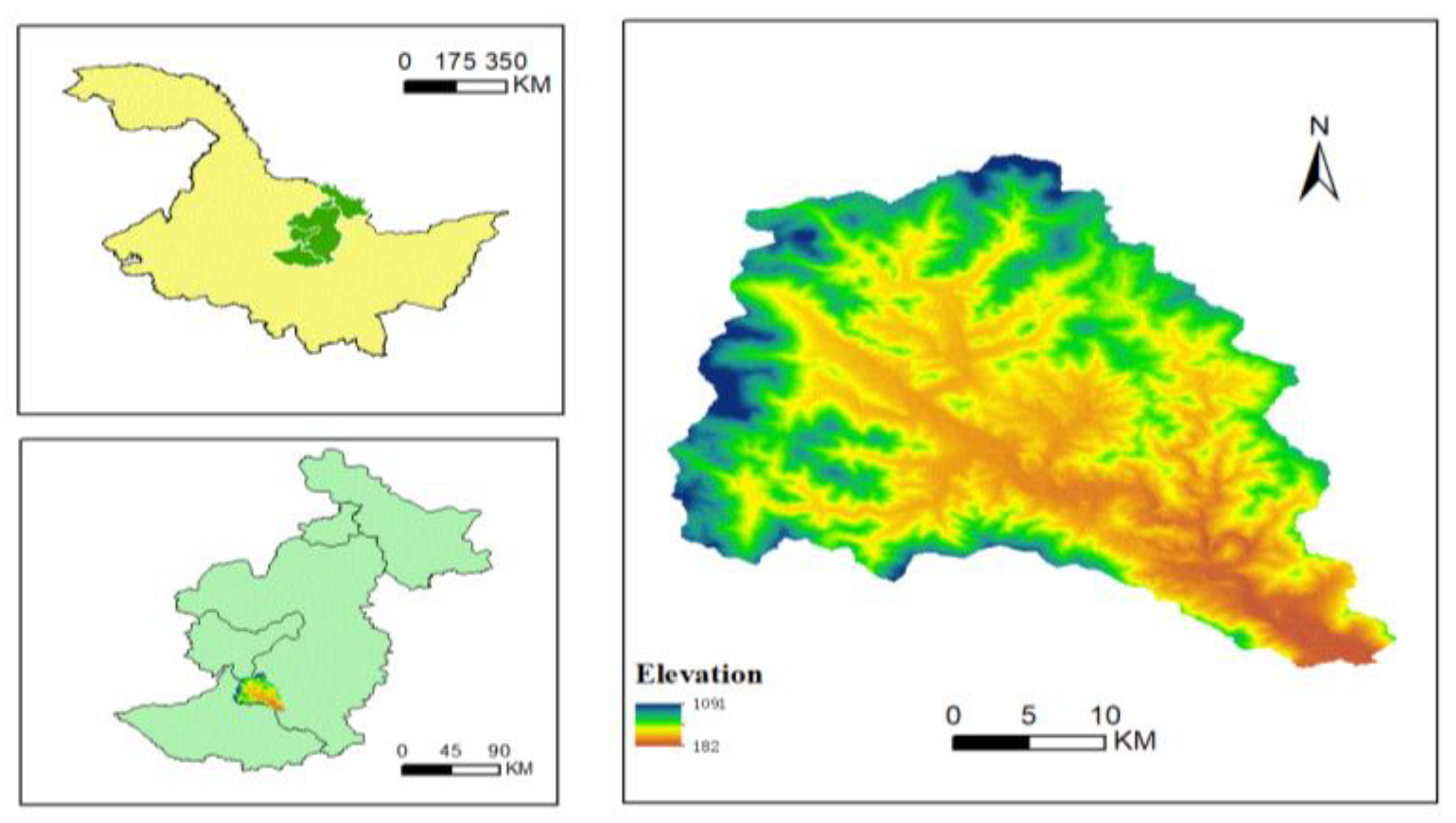
Figure 2.
Long-tail distribution of daily precipitation with heavy rainfall events (≥25 mm) highlighted.
Figure 2.
Long-tail distribution of daily precipitation with heavy rainfall events (≥25 mm) highlighted.
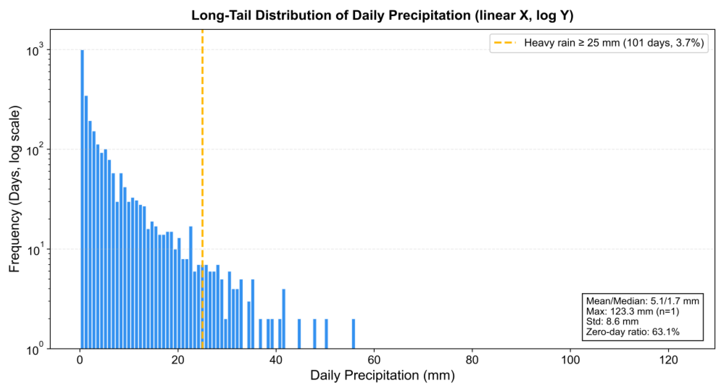
Figure 8.
Multi-level precipitation forecast network.
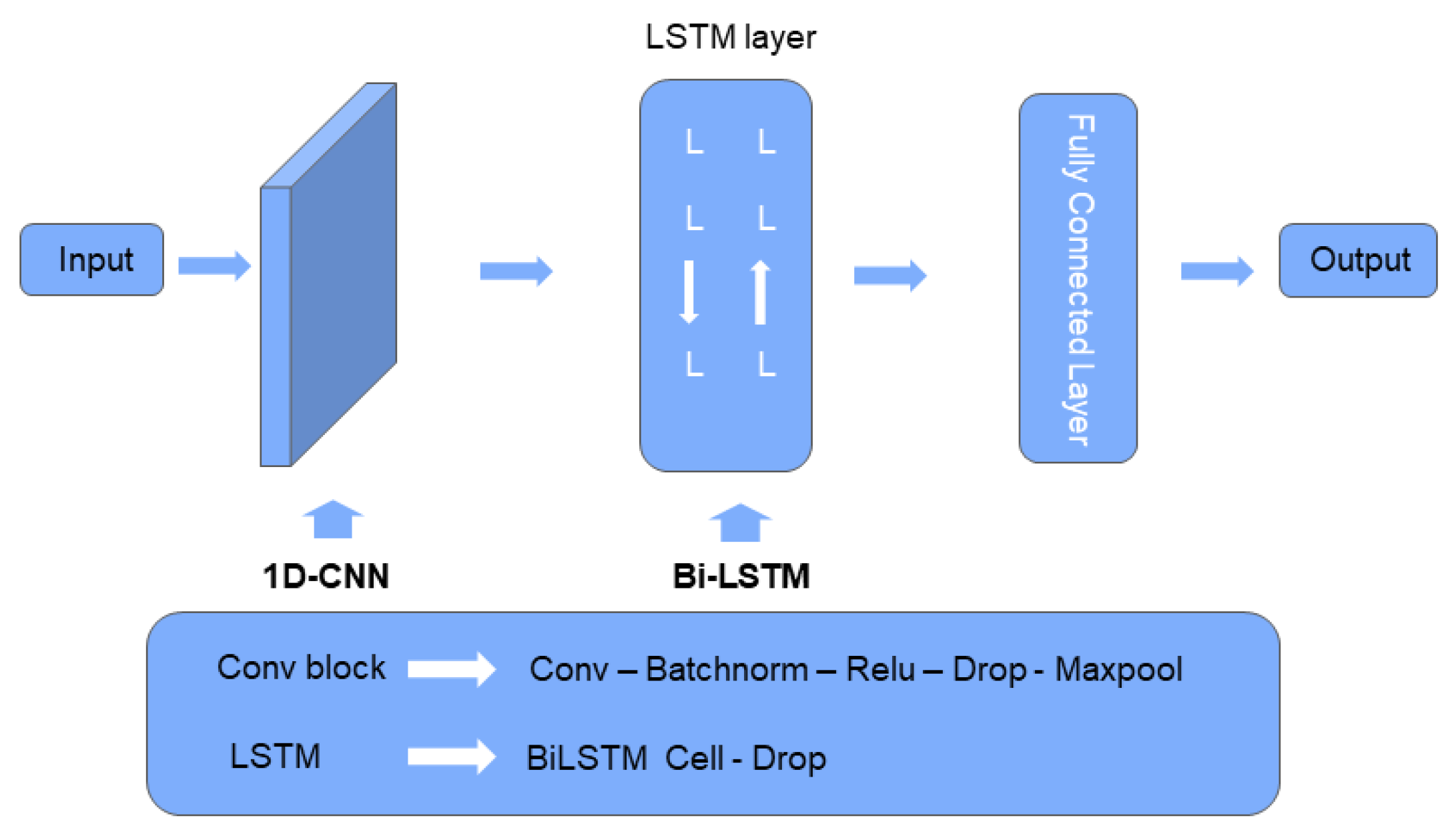
Figure 9.
Schematic Diagram of the Enhanced Transformer Architecture.
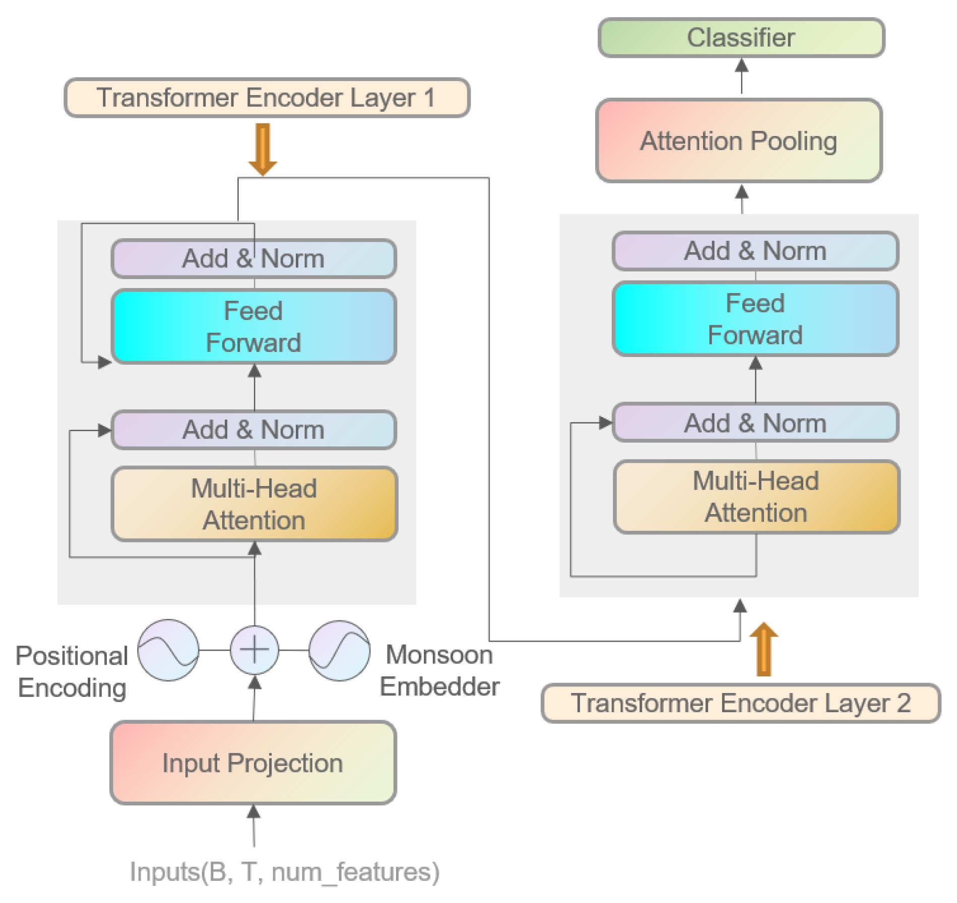
Table 1.
Temporal Splitting Scheme for Three-Fold Cross-Validation.
| Fold | Training Year Range | Validation Year Range | Data Coverage |
|---|---|---|---|
| Fold 1 | 1980–1989 | 1990–1992 | Approx 65% |
| Fold 2 | 1980–1991 | 1992–1994 | Approx 70% |
| Fold 3 | 1980–1993 | 1994–1995 | Approx 75% |
Table 2.
Comparative Results on Three-Class Forecasting Task
| model | augment | test_f1_heavy | delta_f1 | test_recall_heavy | test_auc_score |
|---|---|---|---|---|---|
| CNN-LSTM | None augment | 0.1053 | 0.0241 | 0.15 | 0.6412 |
| CNN-LSTM | SMOTE | 0.1186 | 0.0187 | 0.1825 | 0.6578 |
| CNN-LSTM | ADASYN | 0.0954 | 0.0304 | 0.1427 | 0.6364 |
| CNN-LSTM | GAN | 0.1053 | 0.0241 | 0.2488 | 0.6451 |
| Transformer | None augment | 0.087 | 0.0373 | 0.75 | 0.6289 |
| Transformer | ADASYN | 0 | 0.3035 | 0 | 0.6263 |
| Transformer | SMOTE | 0.125 | 0.0476 | 0.35 | 0.5978 |
| Transformer | GAN | 0.0345 | 0.0181 | 0.1 | 0.636 |
Table 3.
Comparative Results on Two-Class Forecasting Task.
| model | augment | test_f1_heavy | delta_f1 | test_recall_heavy | test_auc_score |
|---|---|---|---|---|---|
| CNN-LSTM | None augment | 0.125 | 0.0127 | 0.45 | 0.8563 |
| CNN-LSTM | SMOTE | 0.0924 | 0.5082 | 0.55 | 0.8198 |
| CNN-LSTM | ADASYN | 0 | 0.9448 | 0 | 0.8614 |
| CNN-LSTM | GAN | 0.0659 | 0.0513 | 0.15 | 0.8573 |
| Transformer | None augment | 0.1345 | 0.0154 | 0.4 | 0.8755 |
| Transformer | ADASYN | 0 | 0.9448 | 0 | 0.8532 |
| Transformer | SMOTE | 0.0709 | 0.7505 | 0.45 | 0.8253 |
| Transformer | GAN | 0.0905 | 0.0067 | 0.55 | 0.8391 |
Disclaimer/Publisher’s Note: The statements, opinions and data contained in all publications are solely those of the individual author(s) and contributor(s) and not of MDPI and/or the editor(s). MDPI and/or the editor(s) disclaim responsibility for any injury to people or property resulting from any ideas, methods, instructions or products referred to in the content. |
© 2025 by the authors. Licensee MDPI, Basel, Switzerland. This article is an open access article distributed under the terms and conditions of the Creative Commons Attribution (CC BY) license (http://creativecommons.org/licenses/by/4.0/).
Copyright: This open access article is published under a Creative Commons CC BY 4.0 license, which permit the free download, distribution, and reuse, provided that the author and preprint are cited in any reuse.


