
Submitted:
15 October 2025
Posted:
16 October 2025
You are already at the latest version
Abstract
In this study, a machine learning-based quality control algorithm for heavy rainfall was developed by integrating automatic weather station observations with remote sensing data, minute-level data, and metadata. Based on heavy rainfall samples from 1 June 2022 to 31 December 2024, the performances of four gradient boosting models (XGBoost, LightGBM, CatBoost, and GBRT) significantly outperformed conventional method, with XGBoost in particular achieving an increase in precision by 0.110, recall by 0.162, and F1-score by 0.140. This performance gain is attributed to the models’ ability to effectively learn nonlinear features from complex multi-source data, thereby reducing both false alarms and missed detections of anomalous rainfall events. The radar composite reflectivity, satellite cloud-top temperature, and minute-level precipitation were identified as dominant contributors to model predictions. The integration of multi-sensor observations effectively addressed limitations inherent in conventional threshold-based approaches. Through SHAP-based interpretability analysis, the model’s decision logic was shown to align with meteorological physical principles. Characteristic patterns such as combinations of low radar reflectivity and elevated cloud-top temperatures were flagged as anomalous rainfall events, typically corresponding to manual operational errors. Moreover, the model identified anomalous minute-level precipitation extremes to be critical signals for detecting instrument malfunctions, data encoding and transmission errors. The physical consistency of the model’s reasoning enhances its trustworthiness and supports its potential for operational implementation in heavy rainfall quality control.
Keywords:
quality control
; heavy rainfall
; machine learning
; multi-source data
; interpretability
1. Introduction
In surface meteorological observation, precipitation data are regarded as one of the most frequently utilized and critically supportive datasets [1,2,3]. Accurate precipitation data, particularly heavy rainfall data, is widely employed in weather forecasting, climate change studies, and numerical model assimilation [3,4,5]. These data also serve as essential decision-making bases for key societal sectors such as agricultural production, water resource management, and ecological security [6,7,8].
With the continuous construction and expansion of Chinese surface observation network, the number of automatic weather stations (AWSs) has exceeded 70,000, significantly improving observational coverage and density [9]. However, more than 95% of them are unmanned. Without dedicated on-site maintenance or backup precipitation observation devices, these unmanned stations often suffer from operational instability and non-standard installation, making them prone to various data quality anomalies [10,11,12].
Currently, the quality control (QC) of surface precipitation data in China primarily relies on traditional methods, such as regional extreme value checks, temporal consistency checks, and spatial consistency comparisons between stations [13,14,15,16]. For instance, the Meteorological Data Operation System (MDOS) of the China Meteorological Administration (CMA) employs a combination of file-level rapid QC, hourly batch QC, and daily data QC to achieve automated processing [17]. However, these methods still exhibit high rates of missed detections and false alarms in cases such as isolated heavy rainfall caused by human operational errors or continuous large precipitation values resulting from equipment malfunctions [18,19,20,21,22]. Although manual review can serve as an effective supplement to automated QC, it is typically conducted several hours after data arrival, making it difficult to meet the timeliness requirements for real-time heavy rainfall monitoring and emergency response [17,23].
With the advancement of ground- and satellite-based observation technologies and the explosive growth of meteorological data, multi-source data collaborative QC for precipitation has demonstrated significant advantages [24,25,26,27,28]. Compared with traditional approaches, these methods integrate various observational data, including Doppler weather radar, geostationary meteorological satellite, and weather detector, effectively reducing the false alarm rate in anomaly detection [24,25,26]. Furthermore, multi-source collaborative QC also contributes positively to the quality improvement of hydrological precipitation data [27,28]. However, multi-source collaborative QC methods rely mainly on statistically based static thresholds and have not yet fully exploited the complementary potential of multi-source data. Therefore, their optimization and fusion mechanisms require further exploration.
Machine learning methods can automatically learn discriminative features from historical data and identify complex patterns that are difficult to capture using static thresholds [21,29,30]. This capability enables the establishment of more robust and complex nonlinear mapping relationships between precipitation data and other multi-source observations. Additionally, through model structure design or ensemble learning strategies, machine learning can adaptively adjust the contribution weights of various inputs, effectively integrating the strengths of different data sources [31,32]. For example, machine learning algorithms such as decision trees, K-nearest neighbors, and isolation forests have been applied to classify outliers, significantly improving the detection accuracy of anomalous precipitation data [33,34,35,36]. Neural networks have been used to construct real-time precipitation confidence intervals, enabling model adaptation across spatial and seasonal variations [37,38]. By incorporating topographic elevation data through deep neural networks and multi-scale ensemble learning techniques, the capability to detect precipitation quality anomalies in data-sparse regions such as coastal and mountainous areas has been enhanced [39].
To address the missed detections and false alarms in the heavy rainfall QC caused by human operational errors, equipment malfunctions, and other non-meteorological factors, a machine learning-based algorithm was developed in this study. The proposed algorithm employed multi-source data (AWS, radar, satellite, and metadata) from 1 June 2022 to 31 December 2024 and was modeled using advanced machine learning techniques. Furthermore, interpretability analysis was performed on the model results to enhance their reliability, thereby providing more dependable decision support for weather forecasting operations and related public welfare sectors.
2. Data and Methods
2.1. Data
The data employed in this study are categorized into three primary types: (1) surface observational data (including hour-level and minute-level data), (2) remote sensing data, and (3) metadata. The dataset covers a two-year period from 1 June 2022 to 31 May 2024 for model training and testing, and a subsequent six-month period from 1 June to 31 December 2024 for validation, with the spatial scope encompassing the entirety of China. For the development of a QC algorithm for heavy rainfall, this study focused on surface observational data with hourly precipitation exceeding 40 mm. The corresponding remote sensing data and metadata from these events were selectively extracted for analysis, with a total dataset of over 127,000 records.
2.1.1. Surface Observational Data
The surface observational data were obtained from a CMA-maintained network comprising national and provincial AWSs [6,9,17], with a station density higher in the eastern and southern regions than in the western and northern areas (Figure 1). Thirteen hour-level parameters, including hourly precipitation (PRE_1h), temperature (TEM), dew point temperature (DPT), atmospheric pressure (PRS), 3-hour atmospheric pressure change (PRS_Change_3h), 24-hour atmospheric pressure change (PRS_Change_24h), relative humidity (RHU), instantaneous wind speed (WIN_S_INST), maximum instantaneous wind speed in 1 hour (WIN_S_INST_Max), 10-minute average wind speed (WIN_S_Avg_10mi), instantaneous wind direction (WIN_D_INST), direction of maximum instantaneous wind speed in 1 hour (WIN_D_INST_Max), and 10-minute average wind direction (WIN_D_Avg_10mi), were extracted as input features for the models.
In addition to the hour-level surface observational data, minute-level precipitation data were also incorporated in this study. Due to the substantial volume of the minute-level data, feature extraction processes were performed to characterize its mean, extremums, and degree of dispersion. The average (PRE_1m_Ave), maximum (PRE_1m_Max), minimum (PRE_1m_Min), and standard deviation (PRE_1m_Std) of all minute-level values in each hour were calculated and used as input features for the models. The average and standard deviation of minute-level precipitation were defined by Equations (1 and 2), respectively.
where represents the
minute-level precipitation value of the i-th sample, and N
indicates the record number of minute-level precipitation in this hour.
2.1.2. Remote Sensing Data
The remote sensing data utilized in this study comprised the composite reflectivity (CR) mapping product from Doppler weather radars and the cloud-top temperature (CTT) product retrieved from the Fengyun-4B (FY-4B) geostationary meteorological satellite. Both products were quality-controlled data [40,41].
The CR mapping product is generated through periodic volume scans conducted by individual radar stations [42]. Base data, such as reflectivity, are transmitted in real time to processing centers, where they undergo rigorous QC algorithms to remove ground clutter and electromagnetic interference. The polar coordinate data from each single radar are then interpolated onto a unified latitude–longitude grid. Finally, a “maximum reflectivity“ fusion algorithm is applied to produce the composite reflectivity mapping product. This mapping product is built upon a foundation of unified calibration across all radars in China, ensuring consistency and comparability of data from different stations. It provides complete coverage of China at high spatiotemporal resolutions of 6 minutes and 0.01°.
The FY-4B satellite-derived cloud-top temperature product is retrieved via multi-channel remote sensing detection [43]. The satellite employs an Advanced Geosynchronous Radiation Imager to observe specific infrared channels, such as the long-wave infrared window channels at 10.3-11.3 μm and 11.5-12.5 μm. The raw radiance emitted from cloud tops is acquired and radiometrically calibrated to obtain accurate top-of-atmosphere radiance values [44]. Based on Planck’s blackbody radiation law, these radiance values are subsequently inverted into cloud-top temperatures. The geographic projection coordinates from the satellite data are computed based on the World Geodetic System-1984 Coordinate System [45], and the row and column numbers of the detection products are thereby converted into geographical latitude and longitude values. This product covers East Asia with temporal and spatial resolutions of 15 minutes and ~4 km, respectively.
Radar and satellite data exhibit strong complementary characteristics. Radar observations provide high spatiotemporal resolution, enabling effective monitoring of the initiation and evolution of meso- and micro-scale severe convective systems, thereby compensating for the limitations of satellites in detailed monitoring. Satellite observations are not constrained by topography and can cover regions such as oceans, plateaus, and mountains, where radar deployment is challenging, thus mitigating radar blind zones in areas with complex topography. By integrating radar and satellite data, the technical advantages of both ground-based and satellite-based remote sensing can be leveraged, enhancing the reliability of heavy rainfall QC.
2.1.3. Metadata
Metadata are defined as “data about data”, which describe the context and provenance of the data and are essential for their correct interpretation and use. Key components include station location, instrument specifications, measurement method, etc. [46]
The acquisition of metadata is a systematic process. During station construction, geographical and instrumental information are surveyed and recorded. Subsequently, identifiers and timestamps are embedded by the data loggers during data collection and transmission. Finally, processing logs are integrated through standardized formats in processing and archiving. In this study, altitude (Alti), station level, and measurement method were selected as the input features for the models.
2.2. Feature Engineering
2.2.1. Data Matching
Hourly precipitation data represent the cumulative rainfall during the one-hour period immediately preceding each hour (e.g., the precipitation recorded at 06:00 corresponds to the accumulated rainfall between 05:00 and 06:00). However, remote sensing data sources—with temporal resolutions of 6 minutes for radar and 15 minutes for satellite—exhibit significantly higher temporal resolution than hourly precipitation data. This discrepancy in temporal scale leads to fundamental inconsistencies when directly performing grid-to-grid matching in these heterogeneous datasets.
A sliding average temporal window method was applied to process the remote sensing data [47]. For each hourly precipitation value, all available radar or satellite gridded observations within the preceding one-hour window were extracted. The average of these high-resolution values was then computed (A schematic diagram is shown in Figure 2) and matched with the hourly precipitation data. This method effectively aligns the high-frequency remote sensing data with the hourly precipitation observations on a consistent temporal scale, thus achieving temporal consistency for multi-source data matching.
For spatial matching, a spatial nearest-neighbor averaging method was employed in this study [48]. Centered on the latitude and longitude coordinates of each AWS, the CR and CTT gridded data within the surrounding area were searched. The arithmetic mean of the five nearest grid points was then calculated and used as the remote sensing observation values matched to the hourly precipitation data.
The utilization of multiple grid points within a defined spatial domain for averaging is motivated by practical considerations regarding spatial representation and error minimization. During heavy rainfall events, accompanying strong low-level winds can induce horizontal advection of hydrometeors, resulting in a displacement between the precipitation measured at ground stations and the cloud properties observed directly overhead via remote sensing. Relying solely on the single grid value immediately above one AWS may introduce significant mismatches. This method reduced small-scale spatial inconsistencies, thereby providing a more reliable representation of the remote sensing data within the vicinity of the station.
2.2.2. Feature Selection
In high-dimensional datasets, redundancy and multicollinearity among input features are frequently observed [49]. These issues can increase computational complexity, prolong training time, and potentially lead to overfitting, thus reducing model generalization capability and interpretability. Therefore, feature selection is a critical preprocessing step in machine learning. It aims to construct a low-dimensional and efficient feature subset while preserving essential information from the original data. This process enhances model performance and computational efficiency.
This study adopted a strategy based on correlation analysis to systematically eliminate redundant features [50]. The Pearson correlation coefficient matrix was calculated for all pairwise combinations of the input features and a threshold was set to identify highly correlated feature pairs. For each such pair, one of the features was retained while the other was eliminated. This process effectively removed redundant information, ensuring that the final feature subset consists of features with low mutual correlation.
Based on absolute Pearson correlation coefficient analysis (Figure 3) with a threshold of |r| > 0.5, a systematic elimination of redundant features from the initial 22 input features were conducted. This process resulted in the removal of 7 redundant features (Table 1), including altitude (Alti), dew point temperature (DPT), 24-hour pressure change (PRS_Change_24h), instantaneous wind speed (WIN_S_INST), instantaneous wind direction (WIN_D_INST), minute-level precipitation mean (PRE_1m_Ave) and standard deviation (PRE_1m_Std) in an hour . The refined feature set retained 15 core features, achieving a 31.8% reduction in feature dimensionality while fully preserving critical precipitation-related information encompassing dynamic, thermodynamic, moisture, and cloud microphysical characteristics.
2.3. Machine Learning Models
Gradient boosting machine (GBM) is an ensemble learning framework that leverages the collective power of multiple base learners (typically decision trees) [51,52]. It works by iteratively training a sequence of these base learners to enhance prediction performance. This framework is capable of effectively capturing complex non-linear relationships among variables, adapting to datasets of various structures and sizes, and is widely applicable to both regression and classification tasks.
Based on GBM framework, four particularly prominent and widely-used models have emerged: eXtreme Gradient Boosting (XGBoost) [53,54], Light Gradient Boosting Machine (LightGBM) [55], Categorical Boosting (CatBoost) [56,57], and Gradient Boosted Regression Trees (GBRT) [58]. These models exhibit distinct advantages in areas such as training efficiency, handling of missing values, and mitigation of overfitting. In this study, these four advanced models were employed to systematically train and predict on the dataset. To ensure these models achieve their designed performance, hyperparameter optimization was conducted automatically using the Optuna library [59] in Python. This library supports efficient hyperparameter tuning across multiple machine learning models and was utilized to identify optimal parameter configurations.
Since the input data are derived from multiple heterogeneous sources, significant differences are observed in their measurement principles, accuracy, and acquisition environments. Considerable variations are exhibited in the value ranges, distribution characteristics, and systematic biases among different inputs [60]. Therefore, Z-score normalization was applied to preprocess each type of input feature separately, by using the formula given in Equation (3).
where denotes the Z-score of the j-th sample in the i-th feature, represents the observed value of the the j-th sample in the i-th feature, is the mean value of the i-th feature, and is the standard
deviation of the i-th feature.
By subtracting the mean and dividing by the standard deviation, the features were transformed into a unified scale, thereby effectively reducing distribution discrepancies. Z-score normalization prevented certain features from exerting excessive influence on model training due to their large numerical values, while also contributing to accelerated convergence and improved generalization capability.
2.4. Model Performance Metrics
To evaluate model performance, a confusion matrix-based performance metrics employed in this study (Figure 4), utilizing accuracy, precision, recall, and F1-Score as key metrics. These metrics are defined by Equations (4–7), respectively [61,62].
where TP (true positive) denotes the number of samples that are positive and correctly predicted as positive; FN (false negative) refers to the number of samples that are positive but incorrectly predicted as negative; FP (false positive) is the number of samples that are negative but incorrectly predicted as positive; and TN (true negative) represents the number of samples that are negative and correctly predicted as negative.
The “actual value“ in the confusion matrix is obtained from manually corrected hourly precipitation QC results, which are currently regarded as the most accurate benchmark (although its timeliness is relatively poor). Furthermore, by comparing the metrics calculated between the model’s outputs and the actual value against those derived from traditional MDOS results and the same actual value, the proposed GBM machine learning models effectively demonstrate their superiority over current operational QC methods.
2.5. Model Interpretation
SHapley Additive exPlanations (SHAP) is widely regarded as one of the most highly useful tools in model interpretability [63,64]. It is a method founded on cooperative game theory that is used to interpret the predictions generated by machine learning models. The prediction of the black-box model is decomposed into the sum of individual feature effects by calculating each feature’s contribution, and renders the final prediction clear and interpretable. A lower SHAP value indicates a lower feature contribution, whereas a higher value corresponds to a greater contribution. The SHAP value is mathematically defined by Equation (8).
where represents the explanation model, x denotes the input features, and M indicates the number of input features. represents the Shapely values for feature i and denotes the constant output value when all inputs are absent. For each feature, the term is computed
using Equations (9) and (10).
where f represents the black box model. denotes a subset of input features, and is the number of non-zero entires in . represents the expected value of the function and S is the set of non-zero indices in .
SHAP values can be approximated using various methods, such as Kernel SHAP, Deep SHAP, and Tree SHAP. In this study, the Tree SHAP-based approach was employed and implemented via the SHAP library in Python.
3. Results
3.1. Importance Analysis
The analysis of normalized feature importance in the four models for the 15 features revealed that remote sensing data played a dominant role in the predictions, with mean normalized feature importance values of 0.332 for CR and 0.220 for CTT, respectively (Figure 5). Precipitation-related features were consistently identified as stable predictors, where the PRE_1m_Max, PRE_1h, and PRE_1m_Min were identified as subdominant predictive factors, with mean normalized feature importance values of 0.090, 0.064, and 0.056. Moderate contributions were observed from wind speed, wind direction, and TEM, with mean normalized feature importance values ranging from 0.026 to 0.046. In contrast, the importance of RHU, PRS, PRS_Change_3h, and metadata features were relatively low, with normalized feature importance values all below 0.01.
However, distinct model-specific characteristics were observed in the feature weighting in the four models (Figure 6). In the XGBoost model, the ranking of feature importance was observed to be similar to the average of the four models, with remote sensing data identified as the most significant (CR, 0.363; CTT, 0.232), followed by precipitation-related features (PRE_1m_Max, 0.080; PRE_1m_Min, 0.067; PRE_1h, 0.056). Greater sensitivity to wind direction (WIN_S_Avg_10mi, 0.113; WIN_D_INST_Max, 0.051) and wind speed (WIN_S_INST_Max, 0.063; WIN_S_Avg_10mi, 0.056) features were exhibited by the LightGBM model, with these values being significantly elevated compared to other models. A unique pattern was presented by CatBoost, which was identified as the only model where a higher importance was allocated to CTT (0.313) than to CR (0.257). This model was also characterized by a considerably greater emphasis being placed on the WIN_S_INST_Max (0.078). In contrast, an extreme dependence on CR was displayed by the GBRT model, which was attributed a normalized feature importance value of 0.509, accounting for over half of the total feature importance. Concurrently, wind-related features were largely disregarded (normalized feature importance value≤0.006). These discrepancies highlighted the inherent biases of different models in capturing complex feature-target relationships, underscoring that the selection of an appropriate model is critical for the accurate interpretation of feature influences in practical applications.
During the modeling process, feature elimination was performed based on feature importance. Only features whose cumulative contribution exceeded 99.5% after sorting in descending order were retained. This procedure further streamlined the model architecture and improved interpretability, following the initial feature selection outlined in Section 2.2.2.
3.2. Comparison of Performance in Different Models
The performances of the four models in heavy rainfall QC were systematically evaluated by the metrics outlined in Section 2.4. The original dataset was partitioned into training and testing sets at a 7:3 ratio. Comparative analysis of two sets revealed that the performance degradation of the four models was not significant, with observed decreases in F1-scores of 0.045, 0.049, 0.047, and 0.044 respectively, thus indicating no substantial overfitting were detected (Table 2 and Table 3).
High accuracies (accuracy > 0.99) were observed by all models in testing set (Table 3). However, it could be attributed to the significant class imbalance in the precipitation dataset employed, where normal precipitation events (negative samples) substantially outnumbered anomalous precipitation events (positive samples). The identification of true negative samples by the models was relatively easy, resulting in the TN value in Eq. (2) being considerably larger than TP, FP, and FN. Consequently, the accuracies were universally inflated, failing to adequately reflect the capability to detect the critical minority class of anomalous precipitation. In comparison, the precision, recall, and F1-score demonstrated greater diagnostic value in identifying such imbalanced datasets.
According to the results, all evaluated metrics of the four models outperformed those of the MDOS QC (Table 3). The superiority of applying machine learning techniques to multi-source data, particularly remote sensing data, for heavy rainfall QC was effectively highlighted. The highest F1-score (0.816) and recall (0.789) were achieved by XGBoost, indicating its superior comprehensive performance in identifying anomalous precipitation. LightGBM was observed to closely follow, with its F1-score (0.811) nearly matching that of XGBoost, while a slightly higher precision (0.845) was attained. The highest precision (0.849) was recorded by the GBRT model, though its recall was found to be relatively lower. All metrics obtained by the CatBoost model on the test set were noted to be slightly inferior to those of the other three comparative models.
The precision-recall (PR) and receiver operating characteristic (ROC) curves [65] of the four models were observed to be similar (Figure 7). The highest average precisions (APs) of 0.777 were achieved by both XGBoost and CatBoost. Meanwhile, the highest two area under the curves (AUCs) were exhibited by LightGBM and XGBoost, with values of 0.942 and 0.941, respectively. Therefore, through a synthesis of metrics, RP and ROC curves assessment, the XGBoost model was regarded as the preferred high-quality model and was chosen for further study (Section 3.4). Compared to the MDOS, the XGBoost model achieved an increase in precision by 0.110, recall by 0.162, and F1-score by 0.140 in the heavy rainfall QC.
3.3. Model Validation
To evaluate the actual predictive performance of the models, data from 1 June to 31 December 2024 were used as the validation set, with the performance metrics calculated accordingly (Table 4). It was observed that slight decreases in precisions were exhibited by all models on the validation set. Reductions of 0.006, 0.022, 0.010, and 0.025 were recorded for XGBoost, LightGBM, CatBoost, and GBRT, respectively, with more pronounced declines being shown by LightGBM and GBRT. A more substantial overall declines were demonstrated in recalls, with decreases of 0.062, 0.053, 0.066, and 0.056, respectively, and the largest reduction was observed in CatBoost. Influenced by both precisions and recalls, a consistent downward trends in the F1-Score were also presented on the validation set, with declines ranging between 0.037 and 0.043 being exhibited by the four models. The overall degradation in model performance may be attributed to the temporal distribution discrepancy between the validation and training sets, indicating a limited decline in generalization capability when models are confronted with temporally shifted data. Nevertheless, all models are found to significantly outperform the MDOS QC results across all metrics in validation set, suggesting that satisfactory QC capability and practical utility are still maintained in actual prediction.
3.4. Feature Contribution
Rooted in an individualized model interpretation method, SHAP values allow a distinct explanation to be provided for each feature. Figure 8 presents how a feature modulates its own contribution to the model output. In this figure, the color of the dot represents the value of that feature for the review (red: high, blue: low), and the position of the dot is the contribution of the feature on the review helpfulness. Positive SHAP values signify that the feature’s value contributes to the model’s prediction of “anomalous precipitation“, and a larger value indicates a stronger contribution. Conversely, negative SHAP values signify a contribution to the prediction of “normal precipitation“, with a smaller (more negative) value corresponding to a stronger contribution.
CR was regarded as the most discriminative feature in the model (Figure 6a and Figure 8). The SHAP summary plot demonstrated that lower CR values were significantly positively correlated with the probability of a record being classified by the model as “abnormal precipitation“ (Figure 8). Additionally, CR SHAP values exhibited a dependence on CTT and PRE_1h (Figure 9a,d). The samples with CR values below 20 dBZ, combined with either hourly precipitation greater than 70 mm or CTT exceeding 260 K, were strongly classified as “anomalous precipitation” by the model. These phenomena were highly consistent with the physical mechanisms governing heavy rainfall formation. Weak radar echoes imply underdeveloped convective systems and weaker processes of water vapor condensation and hydrometeor growth, which are theoretically insufficient to support precipitation rate greater than 40 mm/h. Consequently, when an observed hourly precipitation with a lower CR, the record is highly likely to be attributed to manual operational errors, such as garden watering, cleaning the gauge without disconnecting communication [20,25,26].
CTT was established as a key indicator in the model (Figure 6a and Figure 8). It showed that samples with elevated CTT (i.e., warmer cloud tops), particularly when combined with either a CR below 20 dBZ or hourly precipitation exceeding 70 mm, were readily classified as anomalous precipitation (Figure 10a,d). From a meteorological perspective, cloud systems capable of generating intense convection are typically characterized by high cloud top heights and low cloud top temperatures. A heavy rainfall event accompanied by a high CTT value is considered suspicious. Such events may be associated with shallow or warm-cloud-dominated systems, which typically lack the dynamic and microphysical conditions necessary for producing substantial rainfall. Similar to the CR SHAP analysis, these phenomena may also be attributed to non-meteorological factors.
The PRE_1m_Max was identified as a critical feature utilized for the model (Figure 6a and Figure 8). SHAP analysis indicated that the model was more likely to classify a precipitation event as anomalous under two scenarios: (1) the PRE_1m_Max was less than 0.5 mm (Figure 8 and Figure 11). This was primarily attributed to a logical inconsistency in the data, as such a low precipitation rate was physically implausible to support the observed hourly precipitation greater than 40 mm. This discrepancy is likely caused by data encoding or transmission errors [22,26]; (2) the PRE_1m_Max exceeded 3.5 mm, particularly when accompanied by either a CR of less than 20 dBZ or a CTT greater than 260 K (Figure 11a,b). An actual heavy rainfall event is composed of several high-intensity minute-scale segments, yet its maximum value usually falls within a reasonable physical range. This anomalously high minute values were likely to be induced by instrumental malfunctions [11,18,22,26], such as the persistent false triggering of a reed switch in a tipping-bucket rain gauge due to metal fatigue or foreign object adhesion, leading to an abnormally high count within a single minute. Additionally, occasional strong electromagnetic interference can also produce such physically implausible extreme peaks [20].
The PRE_1m_Min played a distinctive role in this model (Figure 6a and Figure 8). The SHAP analysis revealed that PRE_1m_Min did not heavily depend on other features (Figure 12). But anomalously low values (particularly negative values) of this feature served as a strong indicator for the model to classify a record as “abnormal precipitation”. As minute precipitation represents an accumulated quantity over a period, its value is inherently non-negative. Therefore, the occurrence of negative values exposes errors in the data encoding or transmission, such as improper sign bit handling or data type conversion errors [22,26]. Thus, it is also established as a sensitive indicator for heavy rainfall QC.
4. Summary and Conclusion
In this study, a machine learning-based QC algorithm for heavy rainfall was developed by integrating AWS observations with radar, satellite, and metadata inputs. Based on heavy rainfall samples from 1 June 2022 to 31 December 2024, performance metrics and interpretability were analyzed on the model outputs. The main conclusions are summarized as follows:
In heavy rainfall QC, the four gradient boosting models (XGBoost, LightGBM, CatBoost, and GBRT) demonstrated a marked improvement over the conventional MDOS method, achieving consistently superior performance in precision, recall, and F1-score. Through a comprehensive evaluation of the performance metrics, PR and ROC curves, the XGBoost model achieved the best overall performance, with precision, recall, and F1-score reaching 0.844, 0.789, and 0.816 on the testing set. Compared to the MDOS, the XGBoost model achieved an increase in precision by 0.110, recall by 0.162, and F1-score by 0.140 in heavy rainfall QC. This finding indicated that gradient boosting-based machine learning algorithms can effectively learn the nonlinear relationships between normal and abnormal precipitation from complex multi-source data. These algorithms significantly improved the identification of challenging QC issues like isolated anomalies and continuous heavy rainfall, reducing both false alarms and missed detections.
The radar, satellite, and minute-level precipitation data were found to play dominant roles in the model’s feature importance. The inclusion of these high-value features overcame the limitations of traditional QC methods that rely on static thresholds and single data sources. Moreover, radar data compensated for the spatiotemporal resolution limitations of satellite observations, while satellite data effectively covered the observational gaps of radar in complex terrain. Through the adaptive learning strategy of the machine learning model, these two data sources achieved complementary advantages and synergistic effects.
Interpretability analysis based on the SHAP method demonstrated that the model’s decision logic was highly consistent with meteorological physical mechanisms. For example, low CR or high CTT generally indicated weak precipitation or underdeveloped convective clouds. Heavy rainfall records associated with such features were accurately identified as anomalous by the model, which corresponds to manual operational errors (e.g., garden watering, cleaning the gauge without disconnecting communication) or other non-meteorological factors. Furthermore, anomalous minute-level precipitation extremes were confirmed by the model as key indicators for identifying instrument malfunctions (e.g. the persistent false triggering of a reed switch in a tipping-bucket rain gauge due to metal fatigue or foreign object adhesion), data encoding and transmission errors. This alignment between the decision logic mechanism and physical principles enhances the reliability of the model results and makes the decision process transparent and interpretable for forecasters, demonstrating strong potential for operational application.
Author Contributions
Conceptualization, H.S. and Q.Z.; methodology, H.S., Q.Z., L.S., C.L., and S.Q.; software, H.S. and Y.H.; validation, H.S. and M.X.; formal analysis, H.S. and M.X.; investigation, H.S. and Q.H.; resources, H.S. and Y.G.; data curation, H.S.; writing—original draft preparation, H.S.; writing—review and editing, H.S., Q.Z., L.S., C.L., S.Q., and D.Y.; visualization, H.S. and Y.H.; supervision, L.S., C.L., and S.Q.; project administration, H.S., Q.Z., and L.S.; funding acquisition, H.S., Q.Z., and D.Y. All authors have read and agreed to the published version of the manuscript.
Funding
This research was funded by the National Natural Science Foundation of China, grant number U2342216. The APC was jointly supported by the High-Quality Program of the CMA Meteorological Observation Centre, grant number YZJH24-15 and the Early-Career Research Project of the CMA Meteorological Observation Centre grant number MOCQN202405.
Acknowledgments
This research was supported by data from several institutions. We gratefully acknowledge the CMA Meteorological Observation Centre for providing the radar observation data and surface observational metadata, the National Meteorological Information Centre, CMA for providing the standardized surface observational data, and the National Satellite Meteorological Centre, CMA for providing the FY-4B CTT data.
Conflicts of Interest
The authors declare no conflict of interest.
Abbreviations
The following abbreviations are used in this manuscript:
| Alti | altitude |
| AP | average precision |
| AUC | area under the curve |
| AWS | automatic weather station |
| CatBoost | Categorical Boosting |
| CMA | China Meteorological Administration |
| CR | composite reflectivity |
| CTT | cloud-top temperature |
| DPT | dew point temperature |
| FN | false negative |
| FP | false positive |
| FY-4B | Fengyun-4B |
| GBM | Gradient Boosting Machine |
| GBRT | Gradient Boosted Regression Trees |
| LightGBM | Light Gradient Boosting Machine |
| MDOS | the Meteorological Data Operation System |
| PR | Precision-Recall |
| PRE_1h | hourly precipitation |
| PRE_1m_Ave | average minute-level precipitation in 1 hour |
| PRE_1m_Max | maximum minute-level precipitation in 1 hour |
| PRE_1m_Min | minimum minute-level precipitation in 1 hour |
| PRE_1m_Std | standard deviation of minute-level precipitation in 1 hour |
| PRS | atmospheric pressure |
| PRS_Change_3h | 3-hour atmospheric pressure change |
| PRS_Change_24h | 24-hour atmospheric pressure change |
| QC | quality control |
| RHU | relative humidity |
| ROC | receiver operating characteristic |
| SHAP | SHapley Additive exPlanations |
| TEM | temperature |
| TN | true negative |
| TP | true positive |
| WIN_D_Avg_10mi | 10-minute average wind direction |
| WIN_D_INST | instantaneous wind direction |
| WIN_D_INST_Max | Direction of maximum instantaneous wind speed in 1 hour |
| WIN_S_Avg_10mi | 10-minute average wind speed |
| WIN_S_INST | instantaneous wind speed |
| WIN_S_INST_Max | maximum instantaneous wind speed in 1 hour |
| XGBoost | eXtreme Gradient Boosting |
References
- Eltahir, E.A.; Bras, R.L. Precipitation recycling. Rev. Geophys. 1996, 34(3), 367–378. [CrossRef]
- New, M.; Todd, M.; Hulme, M.; et al. Precipitation measurements and trends in the twentieth century. Int. J. Climatol. 2001, 21(15), 1889–1922.
- Trenberth, K.E. Changes in precipitation with climate change. Clim. Res. 2011, 47(1-2), 123–138.
- Ramage, C.S. Forecasting in meteorology. Bull. Am. Meteorol. Soc. 1993, 74(10), 1863–1872.
- Lien, G.Y.; Kalnay, E.; Miyoshi, T. Effective assimilation of global precipitation: Simulation experiments. Tellus A Dyn. Meteorol. Oceanogr. 2013, 65(1), 19915. [CrossRef]
- Zhang, Q.; Sun, P.; Singh, V.P.; et al. Spatial-temporal precipitation changes (1956–2000) and their implications for agriculture in China. Glob. Planet. Change. 2012, 82, 86–95. [CrossRef]
- Raymondi, R.R.; Cuhaciyan, J.E.; Glick, P.; et al. Water resources: Implications of changes in temperature and precipitation. In Climate Change in the Northwest: Implications for Our Landscapes, Waters, and Communities; Island Press/Center for Resource Economics: Washington, DC, USA, 2013; pp. 41-66.
- Wei, S.; Pan, J.; Liu, X. Landscape Ecological Safety Assessment and Landscape Pattern Optimization in Arid Inland River Basin: Take Ganzhou District as an Example. Hum. Ecol. Risk Assess. 2020, 26(3), 782–806. [CrossRef]
- Yani, Z.; Su, Y.; Zhiqiang, Z.; Jianhua, Q. Quality Control Method for Land Surface Hourly Precipitation Data in China. J. Appl. Meteorol. Sci. 2024, 35(6), 680–691.
- Groisman, P.Y.; Legates, D.R. The accuracy of United States precipitation data. Bull. Am. Meteorol. Soc. 1994, 75(2), 215–228. [CrossRef]
- González-Rouco, J.F.; Jiménez, J.L.; Quesada, V.; Valero, F. Quality control and homogeneity of precipitation data in the southwest of Europe. J. Clim. 2001, 14(5), 964–978. [CrossRef]
- Yang, D.Q.; Kane, D.; Zhang, Z.P.; Legates, D.; Goodison, B. Bias corrections of long-term (1973–2004) daily precipitation data over the northern regions. Geophys. Res. Lett. 2005, 32(19). [CrossRef]
- Kondragunta, C.R.; Shrestha, K.P. Automated Real-Time Operational Rain Gauge Quality-Control Tools in NWS Hydrologic Operations. In Proceedings of the 20th Conf. on Hydrology, American Meteorological Society, Boston, MA, USA, 28 Jan.-2 Feb. 2006.
- Kim, D.; Nelson, B.; Seo, D.J. Characteristics of reprocessed Hydrometeorological Automated Data System (HADS) hourly precipitation data. Weather Forecast. 2009, 24(5), 1287–1296. [CrossRef]
- Schneider, U.; Becker, A.; Finger, P.; et al. GPCC's new land surface precipitation climatology based on quality-controlled in situ data and its role in quantifying the global water cycle. Theor. Appl. Climatol. 2014, 115(1), 15–40. [CrossRef]
- Blenkinsop, S.; Lewis, E.; Chan, S.C.; Fowler, H.J. Quality control of an hourly rainfall dataset and climatology of extremes for the UK. Int. J. Climatol. 2017, 37(2), 722–740. [CrossRef]
- Ren, Z.; Zhang, Z.; Sun, C.; Liu, Y.; Li, J.; Ju, X.; et al. Development of three-step quality control system of real-time observation data from AWS in China. Meteorol. Mon. 2015, 41(10), 1268–1277.
- Habib, E.; Krajewski, W.F.; Kruger, A. Sampling errors of tipping-bucket rain gauge measurements. J. Hydrol. Eng. 2001, 6(2), 159–166. [CrossRef]
- Sieck, L.C.; Burges, S.J.; Steiner, M. Challenges in obtaining reliable measurements of point rainfall. Water Resour. Res. 2007, 43(1). [CrossRef]
- Einfalt, T.; Michaelides, S. Quality control of precipitation data. In Precipitation: Advances in Measurement, Estimation and Prediction, Springer: Berlin, Heidelberg, Germany, 2008; pp. 101–126.
- Yeung, H.Y.; Man, C.; Chan, S.T.; Seed, A. Development of an operational rainfall data quality-control scheme based on radar-raingauge co-kriging analysis. Hydrol. Sci. J. 2014, 59(7), 1293–1307. [CrossRef]
- Lewis, E.; Pritchard, D.; Villalobos-Herrera, R.; Blenkinsop, S.; McClean, F.; Guerreiro, S.; et al. Quality control of a global hourly rainfall dataset. Environ. Model. Softw. 2021, 144, 105169. [CrossRef]
- Mourad, M.; Bertrand-Krajewski, J.L. A method for automatic validation of long time series of data in urban hydrology. Water Sci. Technol. 2002, 45(4-5), 263–270. [CrossRef]
- Zhong, L.; Zhang, Z.; Chen, L.; et al. Application of the Doppler weather radar in real-time quality control of hourly gauge precipitation in eastern China. Atmos. Res. 2016, 172, 109–118. [CrossRef]
- Ośródka, K.; Otop, I.; Szturc, J. Automatic quality control of telemetric rain gauge data providing quantitative quality information (Rain Gauge QC). Atmos. Meas. Tech. 2022, 15, 1-22. [CrossRef]
- Yan, Q.; Zhang, B.; Jiang, Y.; Liu, Y.; Yang, B.; Wang, H. Quality control of hourly rain gauge data based on radar and satellite multi-source data. J. Hydroinform. 2024, 26(5), 1042–1058. [CrossRef]
- Li, S.; Huang, X.; Du, B.; et al. Application of gauge-radar-satellite data in surface precipitation quality control. Meteorol. Atmos. Phys. 2024, 136(5), 33. [CrossRef]
- Sathya, R.; Abraham, A. Comparison of supervised and unsupervised learning algorithms for pattern classification. Int. J. Adv. Res. Artif. Intell. 2013, 2(2), 34–38. [CrossRef]
- Jordan, M.I.; Mitchell, T.M. Machine learning: Trends, perspectives, and prospects. Science. 2015, 349(6245), 255–260. [CrossRef]
- Zhang, S.; Li, X.; Zong, M.; et al. Efficient kNN classification with different numbers of nearest neighbors. IEEE Trans. Neural Netw. Learn. Syst. 2017, 29(5), 1774–1785. [CrossRef]
- Gheibi, O.; Weyns, D.; Quin, F. Applying machine learning in self-adaptive systems: A systematic literature review. ACM Trans. Auton. Adapt. Syst. 2021, 15(3), 1–37.
- Celik, B.; Vanschoren, J. Adaptation strategies for automated machine learning on evolving data. IEEE Trans. Pattern Anal. Mach. Intell. 2021, 43(9), 3067–3078. [CrossRef]
- Martinaitis, S.M.; Cocks, S.B.; Qi, Y.; et al. Understanding winter precipitation impacts on automated gauge observations within a real-time system. J. Hydrometeorol. 2015, 16(6), 2345–2363. [CrossRef]
- Qi, Y.; Martinaitis, S.; Zhang, J.; et al. A real-time automated quality control of hourly rain gauge data based on multiple sensors in MRMS system. J. Hydrometeorol. 2016, 17(6), 1675–1691. [CrossRef]
- Niu, G.; Yang, P.; Zheng, Y.; et al. Automatic quality control of crowdsourced rainfall data with multiple noises: A machine learning approach. Water Resour. Res. 2021, 57(11), e2020WR029121. [CrossRef]
- Cheng, V.; Wang, X.L.; Feng, Y. A quality control system for historical in situ precipitation data. Atmos. Ocean. 2024, 62(4), 271–287. [CrossRef]
- Sciuto, G.; Bonaccorso, B.; Cancelliere, A.; et al. Quality control of daily rainfall data with neural networks. J. Hydrol. 2009, 364(1-2), 13–22. [CrossRef]
- Zhao, Q.; Zhu, Y.; Wan, D.; et al. Research on the data-driven quality control method of hydrological time series data. Water. 2018, 10(12), 1712. [CrossRef]
- Sha, Y.; Gagne, D.J.; West, G.; et al. Deep-learning-based precipitation observation quality control. J. Atmos. Ocean. Technol. 2021, 38(5), 1075–1091. [CrossRef]
- Ośródka, K.; Szturc, J. Improvement in algorithms for quality control of weather radar data (RADVOL-QC system). Atmos. Meas. Tech. Discuss. 2021, 1–21. [CrossRef]
- Song, Z.; Zhao, L.; Ye, Q.; Ren, Y.; Chen, R.; Chen, B. The Reconstruction of FY-4A and FY-4B Cloudless Top-of-Atmosphere Radiation and Full-Coverage Particulate Matter Products Reveals the Influence of Meteorological Factors in Pollution Events. Remote Sens. 2024, 16(18), 3363. [CrossRef]
- Lakshmanan, V.; Smith, T.; Hondl, K.; Stumpf, G.J.; Witt, A. A Real-Time, Three-Dimensional, Rapidly Updating, Heterogeneous Radar Merger Technique for Reflectivity, Velocity, and Derived Products. Wea. Forecasting. 2006, 21(5), 802–823. [CrossRef]
- Yang, J.; Zhang, Z.; Wei, C.; Lu, F.; Guo, Q. Introducing the new generation of Chinese geostationary weather satellites, Fengyun-4. Bull. Am. Meteorol. Soc. 2017, 98(8), 1637–1658. [CrossRef]
- Hodges, K.I.; Chappell, D.W.; Robinson, G.J.; Yang, G. An improved algorithm for generating global window brightness temperatures from multiple satellite infrared imagery. J. Atmos. Ocean. Technol. 2000, 17(10), 1296–1312. [CrossRef]
- Macomber, M.M. World Geodetic System 1984; Defense Mapping Agency: Washington, DC, USA, 1984.
- Overton, A.K. A Guide to the Siting, Exposure and Calibration of Automatic Weather Stations for Synoptic and Climatological Observations; WMO: Geneva, Switzerland, 2007.
- Vergara, V.M.; Abrol, A.; Calhoun, V.D. An average sliding window correlation method for dynamic functional connectivity. Hum. Brain Mapp. 2019, 40(7), 2089–2103. [CrossRef]
- De, S. The use of nearest neighbor methods. Tijdschr. Econ. Soc. Geogr. 1973, 64(5), 307–319.
- Chan, J.Y.L.; Leow, S.M.H.; Bea, K.T.; et al. Mitigating the multicollinearity problem and its machine learning approach: a review. Mathematics. 2022, 10(8), 1283. [CrossRef]
- Chen, P.; Li, F.; Wu, C. Research on intrusion detection method based on Pearson correlation coefficient feature selection algorithm. J. Phys. Conf. Ser. 2021, 1757(1), 012054.
- Natekin, A.; Knoll, A. Gradient boosting machines, a tutorial. Front. Neurorobot. 2013, 7, 21. [CrossRef]
- Ayyadevara, V.K. Gradient Boosting Machine. In Pro machine learning algorithms: A hands-on approach to implementing algorithms in python and R, CA Apress: Berkeley, USA; pp. 117-134.
- Kavzoglu, T.; Teke, A. Advanced Hyperparameter Optimization for Improved Spatial Prediction of Shallow Landslides Using Extreme Gradient Boosting (XGBoost). Bull. Eng. Geol. Environ. 2022, 81(5), 201. [CrossRef]
- Kavzoglu, T.; Teke, A. Predictive Performances of Ensemble Machine Learning Algorithms in Landslide Susceptibility Mapping Using Random Forest, Extreme Gradient Boosting (XGBoost) and Natural Gradient Boosting (NGBoost). Arab. J. Sci. Eng. 2022, 47(6), 7367–7385. [CrossRef]
- Ke, G.; Meng, Q.; Finley, T.; et al. Lightgbm: A highly efficient gradient boosting decision tree. Adv. Neural Inf. Process. Syst. 2017, 30, 3149–3157.
- Prokhorenkova, L.; Gusev, G.; Vorobev, A.; Dorogush, A.V.; Gulin, A. CatBoost: unbiased boosting with categorical features. Adv. Neural Inf. Process. Syst. 2018, 31, 6638–6648.
- Hancock, J.T.; Khoshgoftaar, T.M. CatBoost for Big Data: An Interdisciplinary Review. J. Big Data. 2020, 7(1), 94. [CrossRef]
- Yang, F.; Wang, D.; Xu, F.; Huang, Z.; Tsui, K.L. Lifespan prediction of lithium-ion batteries based on various extracted features and gradient boosting regression tree model. J. Power Sources. 2020, 476, 228654. [CrossRef]
- Lai, L.H.; Lin, Y.L.; Liu, Y.H.; et al. The use of machine learning models with Optuna in disease prediction. Electronics. 2024, 13(23), 4775. [CrossRef]
- Imron, M.A.; Prasetyo, B. Improving algorithm accuracy k-nearest neighbor using z-score normalization and particle swarm optimization to predict customer churn. J. Soft Comput. Explor. 2020, 1(1), 56–62. [CrossRef]
- Helmud, E.; Fitriyani, F.; Romadiana, P. Classification Comparison Performance of Supervised Machine Learning Random Forest and Decision Tree Algorithms Using Confusion Matrix. J. Sisfokom. 2024, 13(1), 92–97. [CrossRef]
- Sathyanarayanan, S.; Tantri, B.R. Confusion matrix-based performance evaluation metrics. Afr. J. Biomed. Res. 2024, 27(4S), 4023–4031.
- Nohara, Y.; Matsumoto, K.; Soejima, H.; Nakashima, N. Explanation of machine learning models using shapley additive explanation and application for real data in hospital. Comput. Methods Programs Biomed. 2022, 214, 106584. [CrossRef]
- Ekanayake, I.U.; Meddage, D.P.P.; Rathnayake, U. A novel approach to explain the black-box nature of machine learning in compressive strength predictions of concrete using Shapley additive explanations (SHAP). Case Stud. Constr. Mater. 2022, 16, e01059. [CrossRef]
- Ozenne, B.; Subtil, F.; Maucort-Boulch, D. The Precision–Recall Curve Overcame the Optimism of the Receiver Operating Characteristic Curve in Rare Diseases. J. Clin. Epidemiol. 2015, 68(8), 855–859. [CrossRef]
Figure 1.
Station density distribution of surface observation network in China.
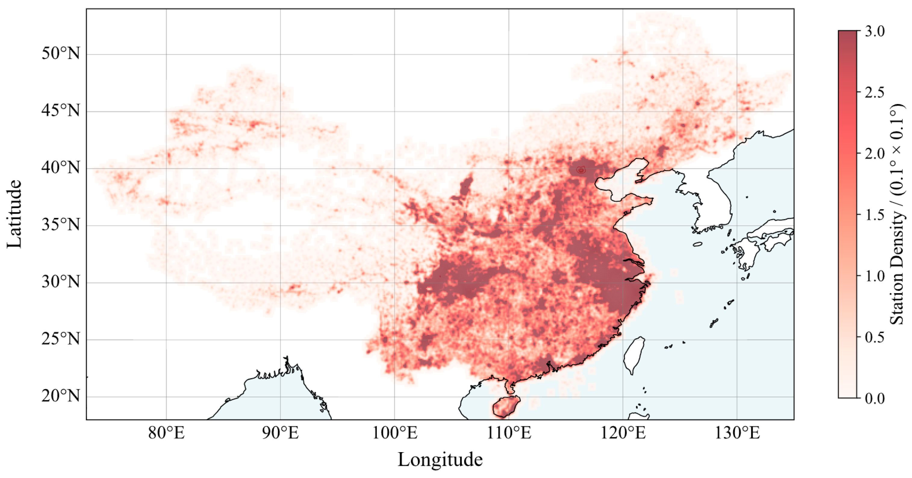
Figure 2.
Temporal matching of hourly precipitation data with remote sensing data through a sliding average temporal window method.
Figure 2.
Temporal matching of hourly precipitation data with remote sensing data through a sliding average temporal window method.
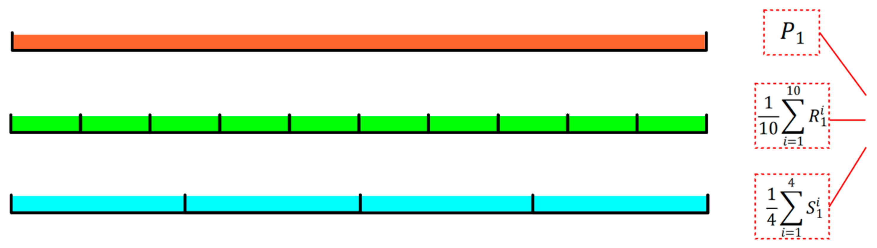
Figure 3.
Absolute Pearson correlation matrix of 22 input features.
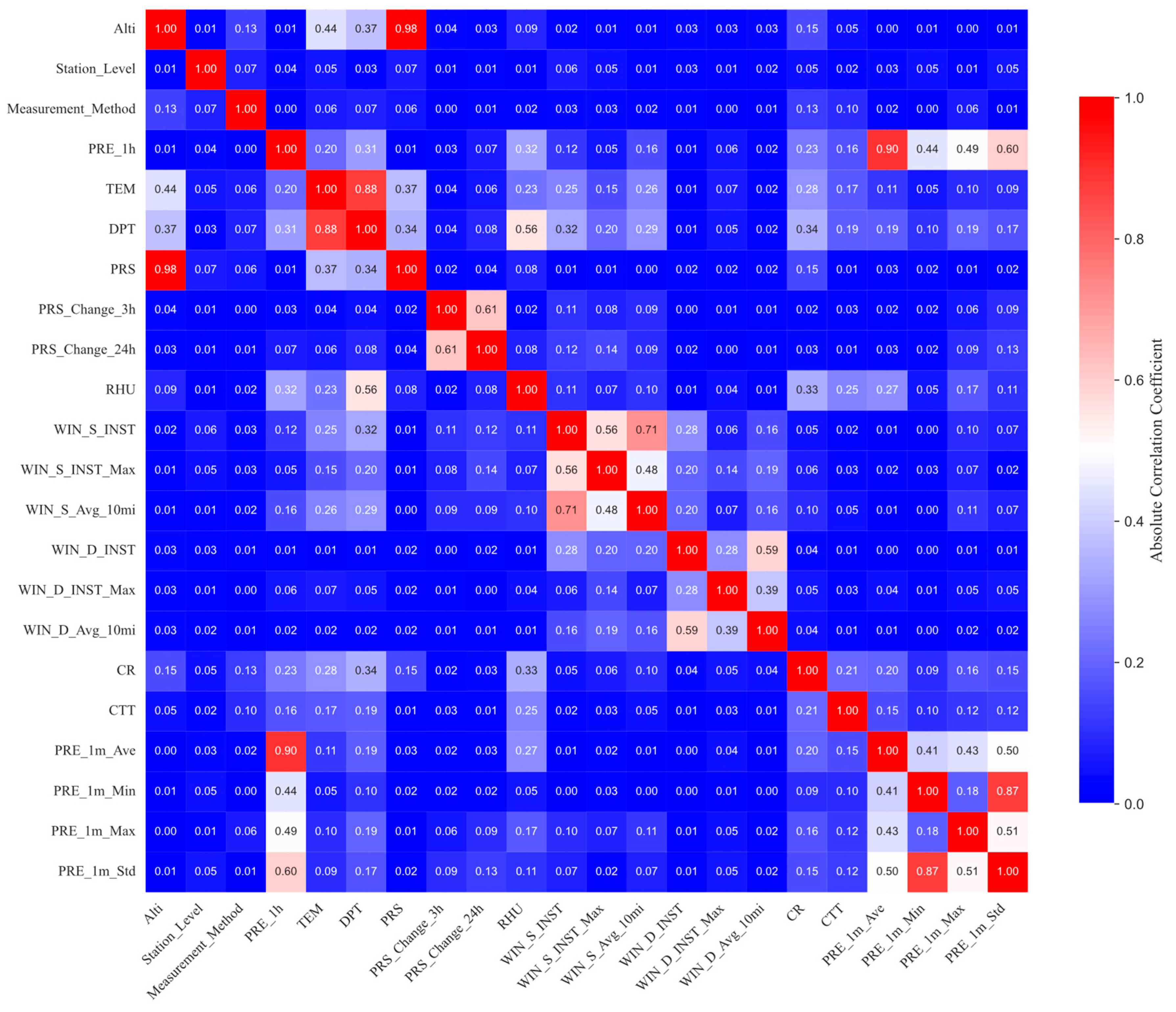
Figure 4.
Schematic of a confusion matrix.
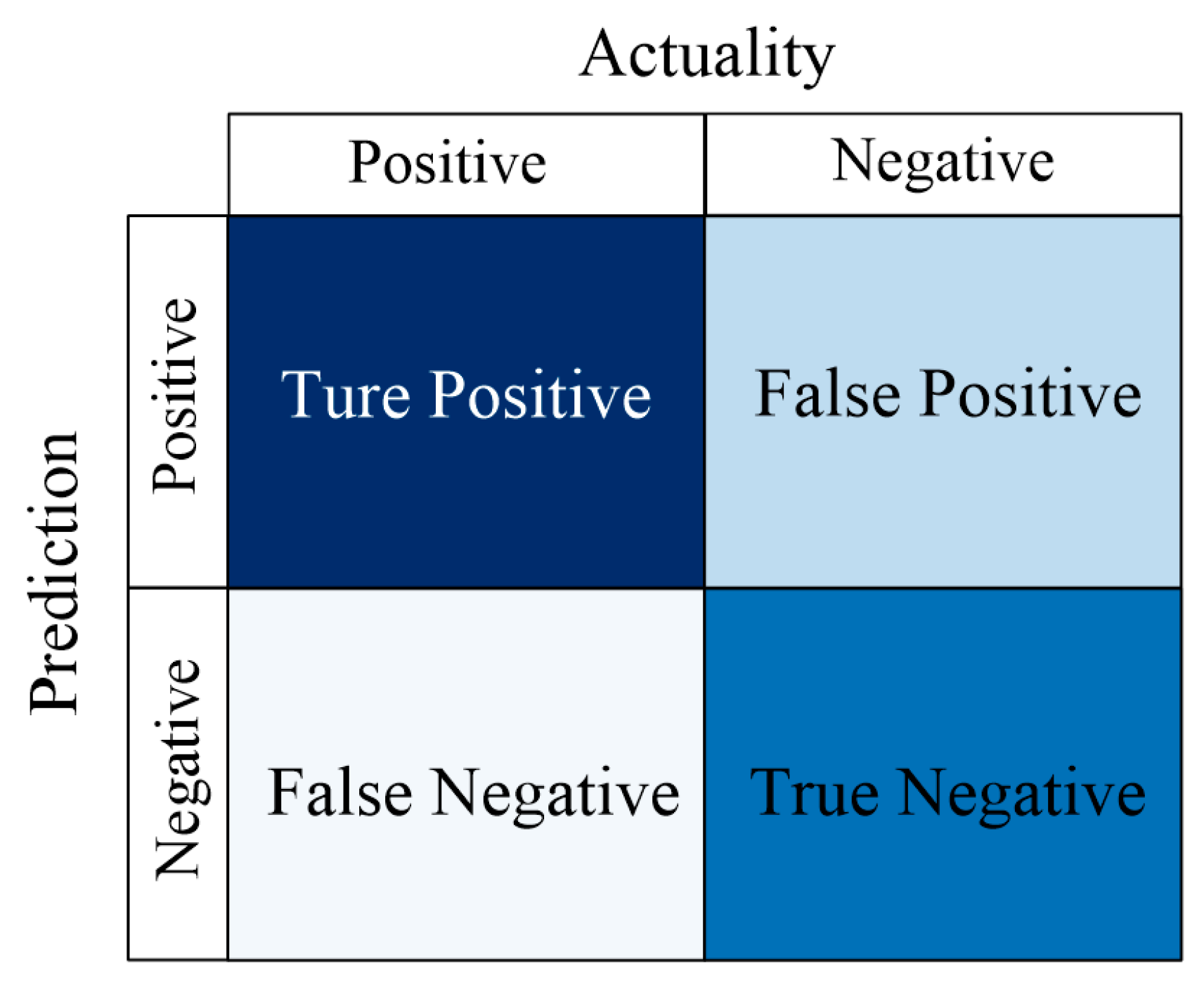
Figure 5.
Normalized feature importance values of the XGBoost, LightGBM, CatBoost and GBRT models.
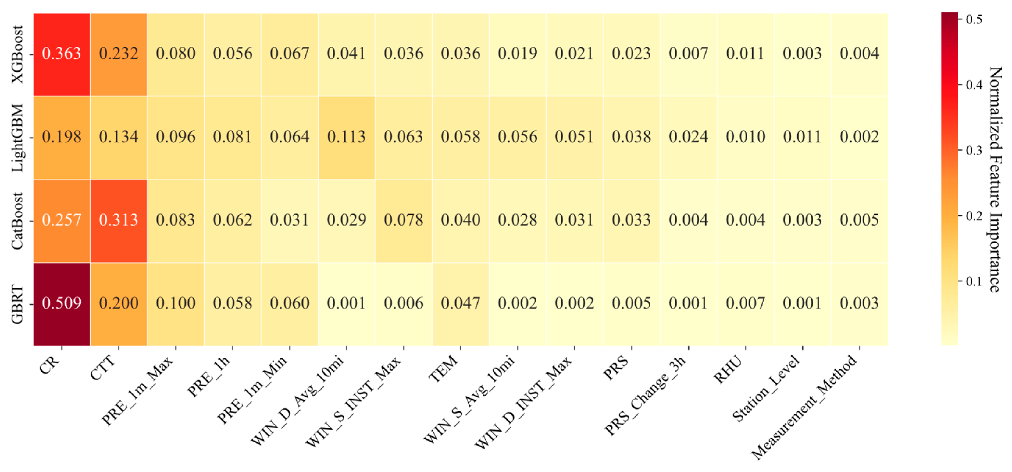
Figure 6.
Normalized feature importance ranking of the (a) XGBoost, (b) LightGBM, (c) CatBoost and (d) GBRT models.
Figure 6.
Normalized feature importance ranking of the (a) XGBoost, (b) LightGBM, (c) CatBoost and (d) GBRT models.
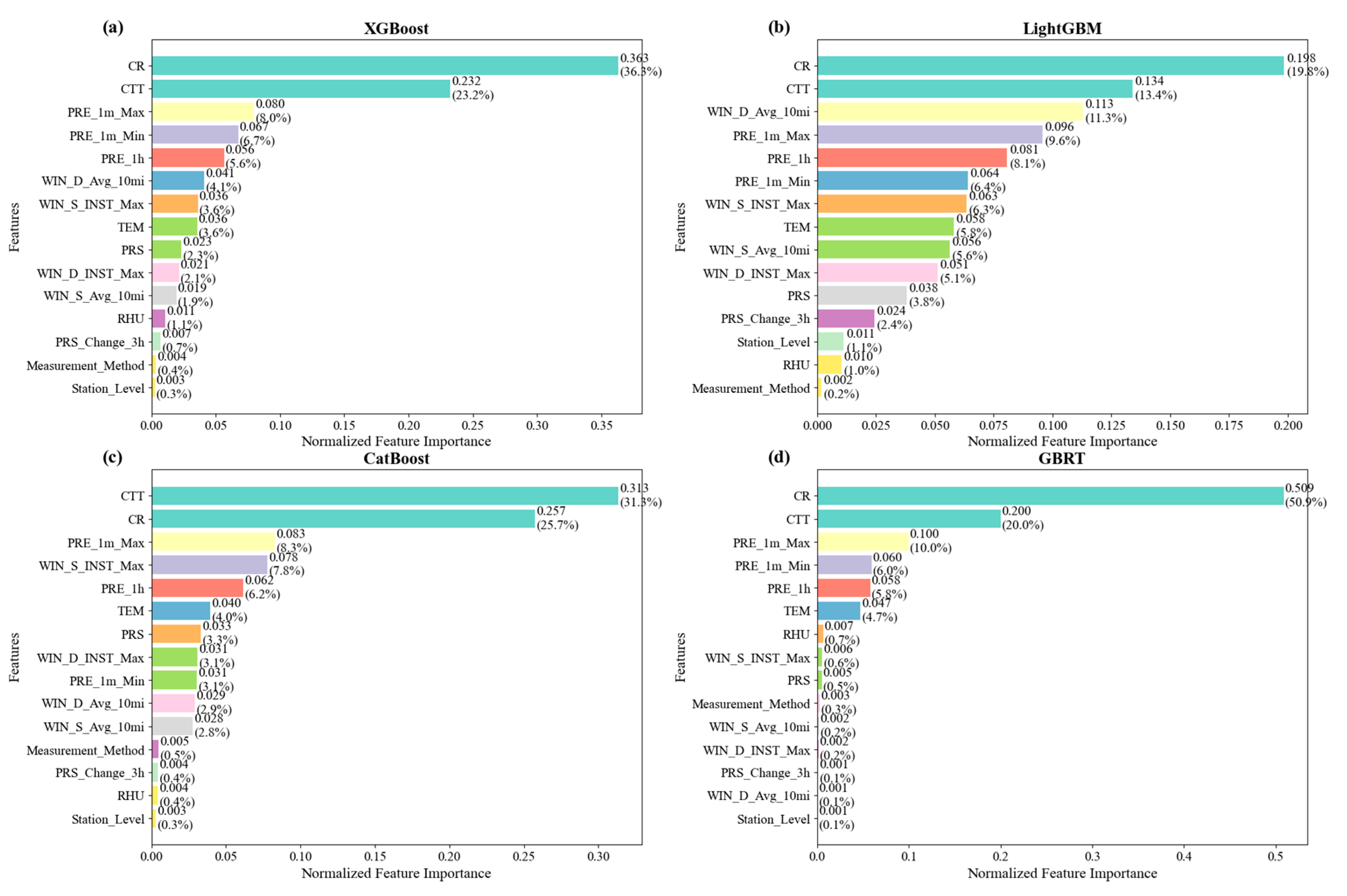
Figure 7.
(a) PR curves with APs and (b) ROC curves with AUCs of the four models.
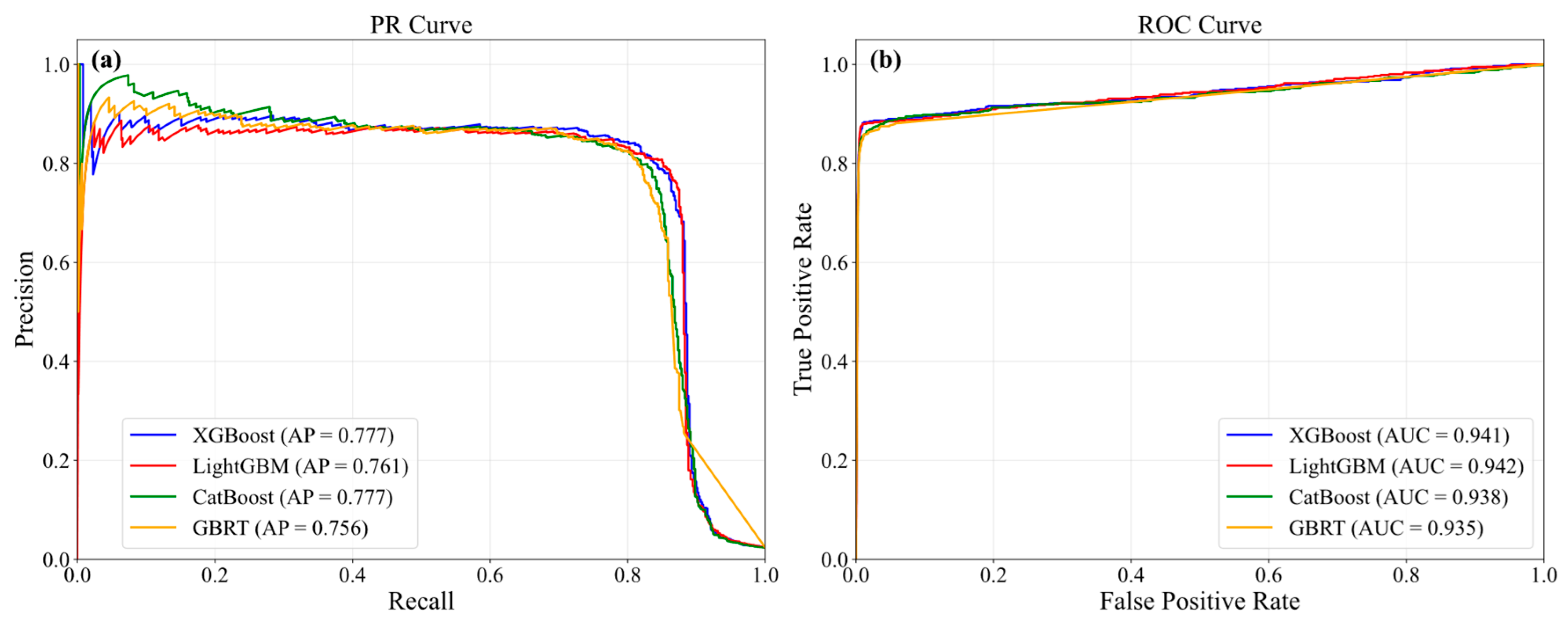
Figure 8.
SHAP summary plot of the XGBoost model.
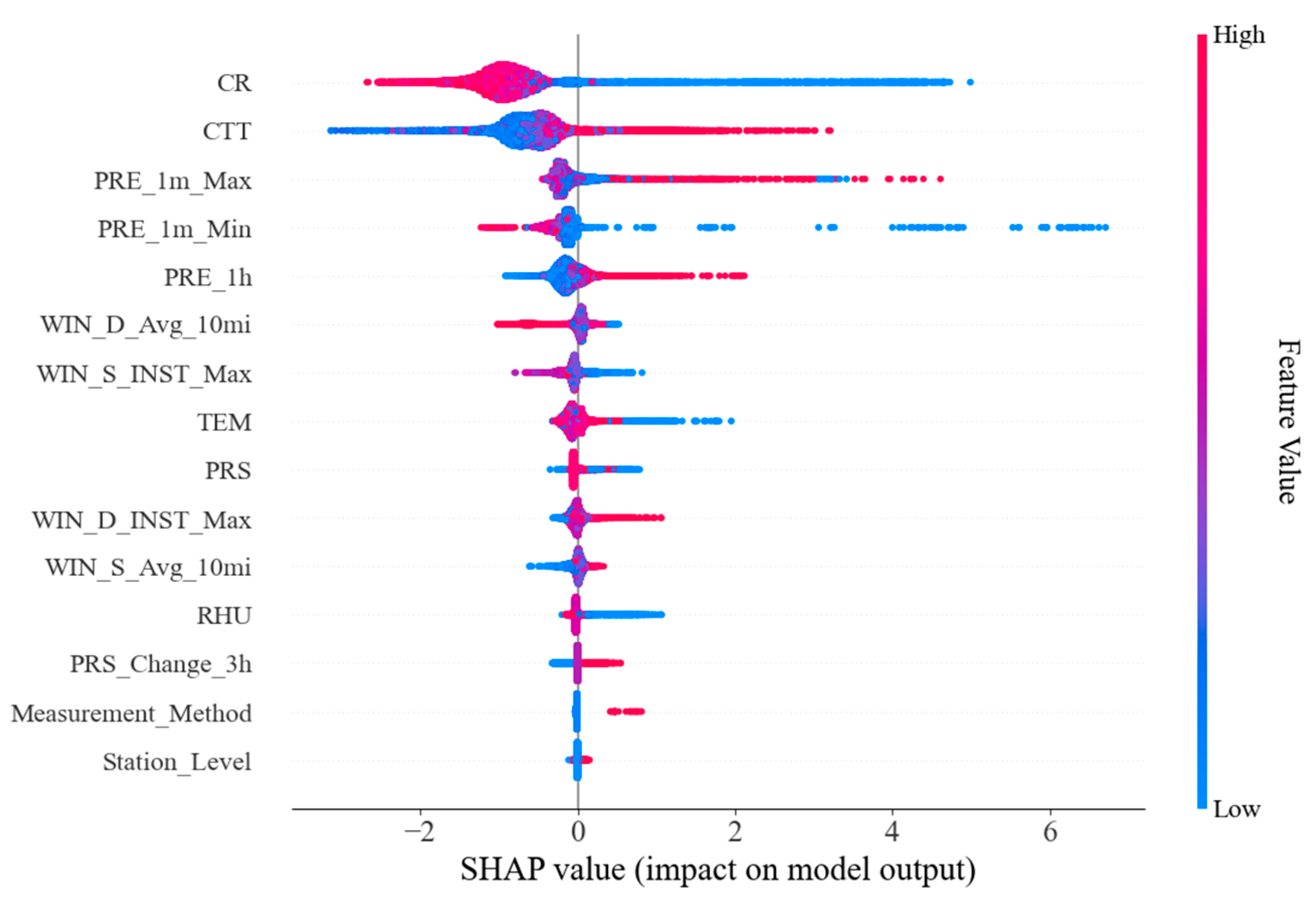
Figure 9.
CR SHAP dependence on (a) CTT, (b) PRE_1m_Max, (c) PRE_1m_Min, (d)PRE_1h, (e) WIN_D_Avg_10mi, (f) WIN_S_INST_Max, (g) TEM, and (h) PRS.
Figure 9.
CR SHAP dependence on (a) CTT, (b) PRE_1m_Max, (c) PRE_1m_Min, (d)PRE_1h, (e) WIN_D_Avg_10mi, (f) WIN_S_INST_Max, (g) TEM, and (h) PRS.
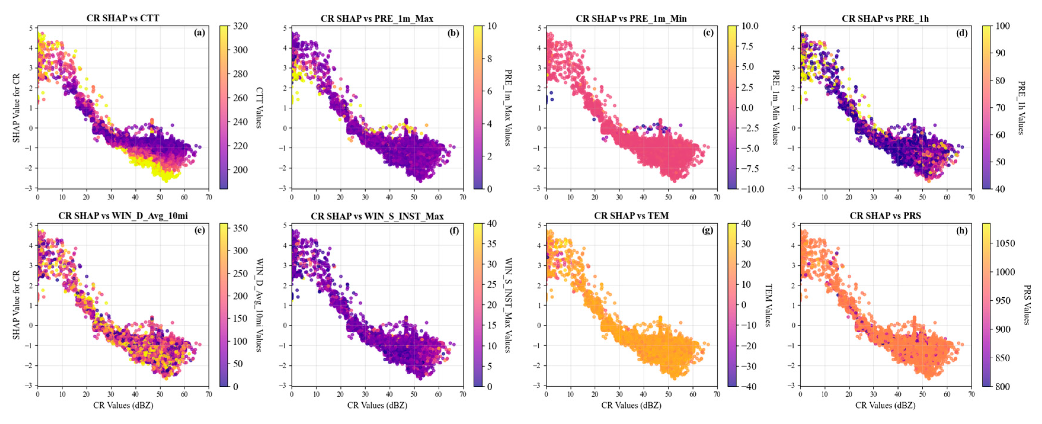
Figure 10.
CTT SHAP dependence on (a) CR, (b) PRE_1m_Max, (c) PRE_1m_Min, (d)PRE_1h, (e) WIN_D_Avg_10mi, (f) WIN_S_INST_Max, (g) TEM, and (h) PRS.
Figure 10.
CTT SHAP dependence on (a) CR, (b) PRE_1m_Max, (c) PRE_1m_Min, (d)PRE_1h, (e) WIN_D_Avg_10mi, (f) WIN_S_INST_Max, (g) TEM, and (h) PRS.
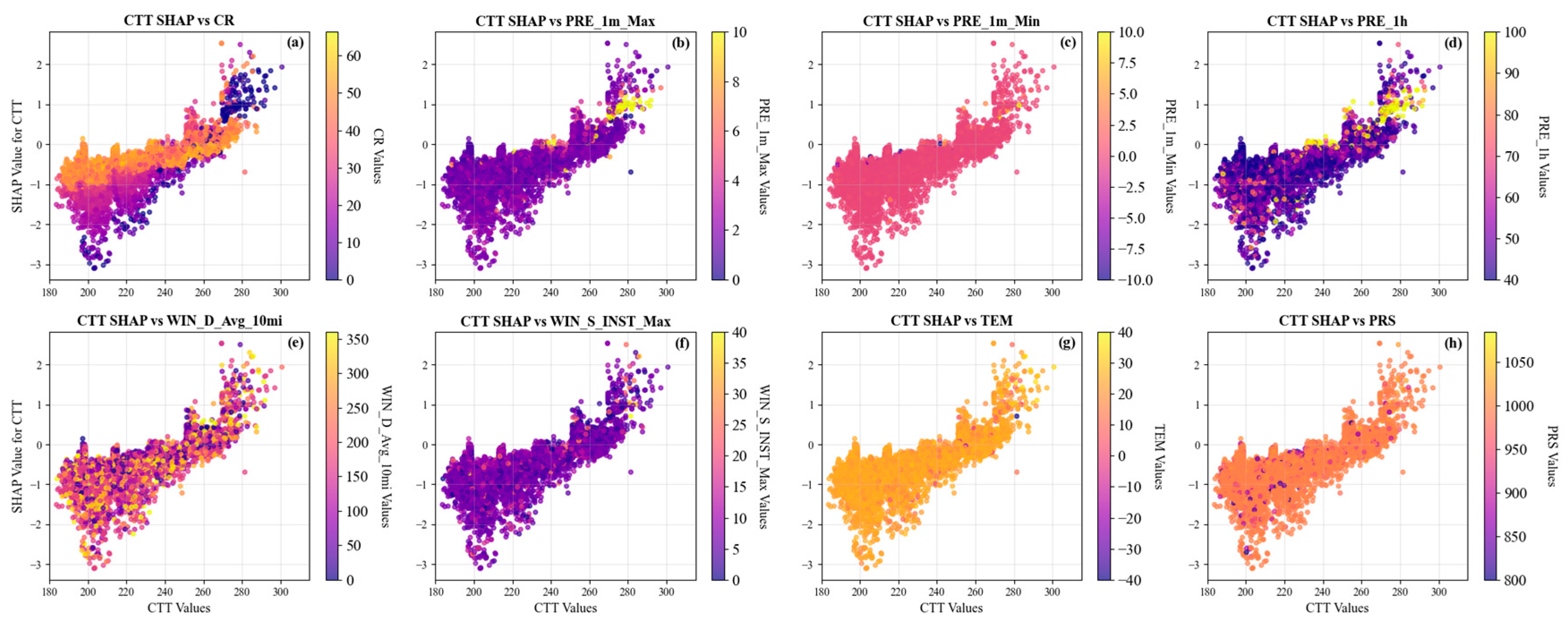
Figure 11.
PRE_1m_Max SHAP dependence on (a) CR, (b) CTT, (c) PRE_1m_Min, (d)PRE_1h, (e) WIN_D_Avg_10mi, (f) WIN_S_INST_Max, (g) TEM, and (h) PRS.
Figure 11.
PRE_1m_Max SHAP dependence on (a) CR, (b) CTT, (c) PRE_1m_Min, (d)PRE_1h, (e) WIN_D_Avg_10mi, (f) WIN_S_INST_Max, (g) TEM, and (h) PRS.
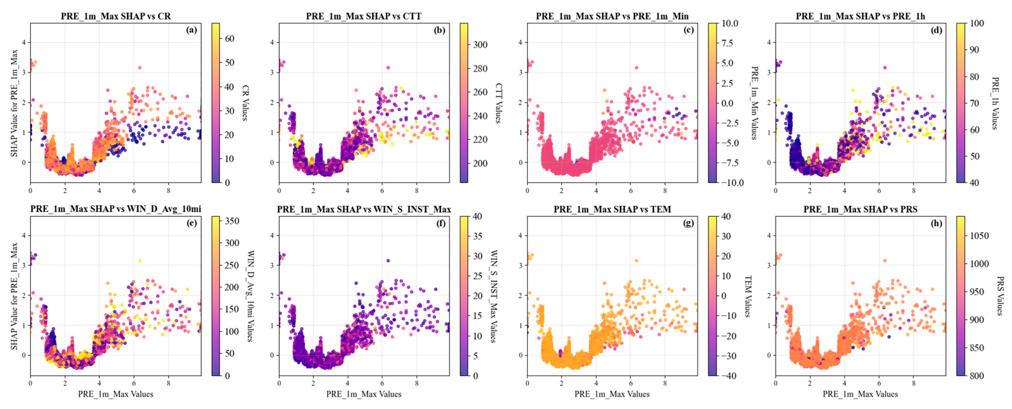
Figure 12.
PRE_1m_Min SHAP dependence on (a) CR, (b) CTT, (c) PRE_1m_Max, (d)PRE_1h, (e) WIN_D_Avg_10mi, (f) WIN_S_INST_Max, (g) TEM, and (h) PRS.
Figure 12.
PRE_1m_Min SHAP dependence on (a) CR, (b) CTT, (c) PRE_1m_Max, (d)PRE_1h, (e) WIN_D_Avg_10mi, (f) WIN_S_INST_Max, (g) TEM, and (h) PRS.
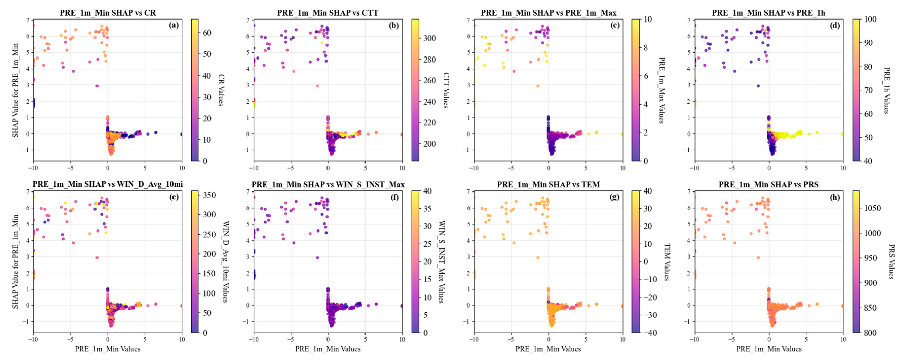

Table 1.
Input features before and after selection.
| Original features | Features after selection | |
|---|---|---|
| MetaData | Alti, Station_Level, Measurement_Method | Station_Level, Measurement_Method |
| Surface | PRE_1h, TEM, DPT, PRS, PRS_Change_3h, PRS_Change_24h, RHU, WIN_S_INST, WIN_S_INST_Max, WIN_S_Avg_10mi, WIN_D_INST, WIN_D_INST_Max, WIN_D_Avg_10mi |
PRE_1h, TEM, PRS, PRS_Change_3h, RHU, WIN_S_INST_Max, WIN_S_Avg_10mi, WIN_D_INST_Max, WIN_D_Avg_10mi |
| Remote Sensing | CR, CTT | CR, CTT |
| Minute precipitation | PRE_1m_Ave, PRE_1m_Min, PRE_1m_Max, PRE_1m_Std | PRE_1m_Min, PRE_1m_Max |
| Total | 22 features | 15 features |
Table 2.
Performance metrics of the four models with control experiment on the training set.
| Accuracy | Precision | Recall | F1-Score | |
|---|---|---|---|---|
| MDOS (control experiment) |
0.986 | 0.709 | 0.619 | 0.661 |
| XGBoost | 0.994 | 0.89 | 0.834 | 0.861 |
| LightGBM | 0.994 | 0.894 | 0.828 | 0.860 |
| CatBoost | 0.992 | 0.885 | 0.804 | 0.843 |
| GBRT | 0.992 | 0.881 | 0.811 | 0.845 |
Table 3.
Performance metrics of the four models with control experiment on the testing set.
| Accuracy | Precision | Recall | F1-Score | |
|---|---|---|---|---|
| MDOS (control experiment) |
0.986 | 0.734 | 0.627 | 0.676 |
| XGBoost | 0.992 | 0.844 | 0.789 | 0.816 |
| LightGBM | 0.991 | 0.845 | 0.78 | 0.811 |
| CatBoost | 0.991 | 0.843 | 0.753 | 0.796 |
| GBRT | 0.991 | 0.849 | 0.758 | 0.801 |
Table 4.
Performance metrics of the four models with control experiment on the validation set.
| Accuracy | Precision | Recall | F1-Score | |
|---|---|---|---|---|
| XGBoost | 0.993 | 0.838 | 0.727 | 0.779 |
| LightGBM | 0.993 | 0.823 | 0.727 | 0.772 |
| CatBoost | 0.992 | 0.833 | 0.687 | 0.753 |
| GBRT | 0.992 | 0.824 | 0.702 | 0.758 |
Disclaimer/Publisher’s Note: The statements, opinions and data contained in all publications are solely those of the individual author(s) and contributor(s) and not of MDPI and/or the editor(s). MDPI and/or the editor(s) disclaim responsibility for any injury to people or property resulting from any ideas, methods, instructions or products referred to in the content. |
© 2025 by the authors. Licensee MDPI, Basel, Switzerland. This article is an open access article distributed under the terms and conditions of the Creative Commons Attribution (CC BY) license (http://creativecommons.org/licenses/by/4.0/).
Copyright: This open access article is published under a Creative Commons CC BY 4.0 license, which permit the free download, distribution, and reuse, provided that the author and preprint are cited in any reuse.


