
Submitted:
02 December 2025
Posted:
03 December 2025
You are already at the latest version
Abstract
Emerging landslides and severe floods highlight the urgent need to analyse and support predictive models and early warning systems. Soil moisture is a crucial parameter and it can now be determined from space with resolution of few tens of meters, potentially leading to a continuous global monitoring of landslide risk. We address this issue by determining the volumetric water content (VWC) of a testbed in Southern Italy (bare soil with significant flood and landslide hazard) through the comparison of two different satellite observations on the same day. In the first observation (Sentinel-1 mission of the European Space Agency, C-band Synthetic Aperture Radar (SAR)), the back-scattered radar signal is used to determine the VWC from the dielectric constant in the microwave range, also using a time-series approach to calibrate the algorithm. In the second observation (hyperspectral PRISMA mission of the Italian Space Agency), the short-wave infrared (SWIR) reflectance spectra are used to calculate the VWC from the spectral weight of a vibrational absorption line of liquid water (wavelengths 1800−1950nm). As the main result, we obtained a Pearson’s correlation coefficient of 0.4 between the VWC values measured with the two techniques and a separate ground-truth confirmation of absolute VWC values in the range 0.10−0.30 within ±0.05. This overlap validates that both SAR and hyperspectral data can be well calibrated and mapped with 30 meter ground resolution - given the absence of artifacts or anomalies in this particular testbed (e.g. vegetation canopy or cloud presence). If hyperspectral data in the SWIR range become more broadly available in the future, our systematic procedure to synchronise these two technologies in both space and time can be further adapted to cross-validate the global high-resolution soil moisture dataset. Ultimately, multi-mission data integration could lead to quasi-real time hydrogeological risk monitoring from space.
Keywords:
earth observation
; synthetic aperture radar
; hyperspectral satellite
; volumetric water content
; soil moisture
; hydrogeological risk monitoring
1. Introduction
Soil moisture monitoring is of crucial importance for numerous Earth and environmental science applications that directly impact the global environment and human society [1,2,3]. Potential applications include weather and climate variability forecasting; drought forecasting [4,5] and monitoring, water resources management and allocation, agricultural production and drought alleviation, monitoring ecosystem response to climate change and, finally, prevention of natural disasters such as fires, landslides [6,7,8], floods [9,10] and sandstorms.
Soil moisture is highly variable on small scales of space and time (e.g. before and after an extreme weather event [11,12]); therefore in recent years, considerable efforts and resources have been dedicated to advancing measurement and monitoring capabilities at a single topographic location while maintaining a global vision over large areas. Traditional soil moisture measurement techniques involve long and expensive campaigns for the installation and maintenance of on-field physical sensors, or for the collection of soil samples to be analyzed in the laboratory [13,14]. Remote sensing techniques using radars or infrared (IR) spectrometers exist, however, these instruments probe an area of a few square meters at a time and therefore, they must be scanned across the entire area with land vehicles, drones, or airplanes. It is evident that soil moisture monitoring from satellites would solve all these problems simultaneously: a satellite providing radar or optical images is typically able to scan entire fractions of the planet in a few hours, with a spatial resolution that can reach a few meters and with data quality continuously improving due to the launch of increasingly sophisticated satellites. The present work concerns innovative methods to calculate soil moisture from latest-generation satellite data, such as those from the PRISMA [15] and Sentinel-1 missions [16], with the aim of monitoring landslide hazard from space. The software tools developed here, however, may well be used for all the other soil moisture monitoring applications mentioned above.
The soil moisture has actually been determined from space since 1978 with passive microwave radiometers, especially with the Advanced Surface Microwave Radiometer (ASMR) instruments onboard United States NASA and Japanese JAXA satellites [17]. Today, several radiometer missions exist (e.g. the SMAP mission of NASA [18]), extending up to the millimeter waves above 100 GHz, and they provide high accuracy and high temporal resolution of six hours but low spatial resolution. The radiometric pixel size is on the order of 1 km2, which may be sufficient for environmental studies and applications in agriculture, but is certainly inadequate for hydrogeological risk monitoring. Active microwave instruments from space feature spatial resolutions of tens of meters or better and are represented almost exclusively by Synthetic Aperture Radar (SAR) satellites emitting radiation in one frequency band in the GHz range. At the time of this study, the Sentinel-1 mission of the ESA is the most suitable satellite, providing publicly available data in the C-band around 5 GHz [19].
Visible and infrared multispectral imaging from satellites has been extensively used to measure the soil moisture qualitatively (in general, darker soils have higher moisture content) with data provided by the NASA mission Landsat [20,21] and by the multispectral instrument MODIS [22]. Reflectance spectroscopy in the SWIR range ( nm) has been employed with ground and airborne spectrometers to determine the VWC with very high precision, as verified by independent direct soil moisture measurements [23,24,25]. Hyperspectral imaging missions provide, for each pixel of an image, a continuous and relatively high-resolution spectral coverage of a given wavelength range that depends on the solar spectrum used as illumination source and on the optical detector technology: silicon detector arrays cover the visible and near-infrared at wavelengths shorter than nm (VIS range), but using HgCdTe or InGaAs detectors allow satellite missions to cover continuously the short-wave IR (SWIR range) nm, beyond which wavelength the solar irradiation spectrum decays below realistic detector noise levels. Hyperspectral imaging satellites have been used in the past mostly for mineral mapping, especially with the Hyperion mission of NASA [26]. Therefore, the use of a hyperspectral imaging satellite (here, the PRISMA mission of the Italian Space Agency, ASI) to determine the VWC quantitatively seems to be a novel approach, not previously attempted, apart from sporadic works on the Hyperion datasets [27].
The aim of the present work is to show that soil moisture can be accurately determined by both SAR and hyperspectral imaging from space, at least in ideal cases. We developed an automated vibrational spectroscopy analysis routine to calculate the VWC map from SWIR spectra of a testbed in Southern Italy with significant landslide hazard. We compare this SWIR VWC map with the VWC map determined from a time-series of SAR images of the same area taken by the Sentinel-1 satellite. The last image of the series has been taken on the same day as the PRISMA image with one hour offset. We also present a ground-truth calibration procedure with soil moisture probes in contact with the ground at an experimental station located in a second testbed. We believe that the frequent soil moisture determination from space in inaccessible terrains could be used as a reliable tool for hydrogeological hazard monitoring that may be impossible to perform in real-time by ground-based SWIR spectroscopy or radar methods, and even with other, more established, terrestrial methods for soil moisture monitoring [28].
2. Materials and Methods
The determination of soil moisture from SAR satellites has been described in detail elsewhere [29], and although we briefly recall our specific SAR method below, we now describe the hyperspectral method more broadly as it was originally devised for this specific work.
2.1. Hyperspectral Imaging with PRISMA
The information-rich quasi-continuous spectrum from the VIS to the SWIR can be analyzed either with purely data-driven techniques using many kinds of classifiers, or with deterministic spectroscopy models that reproduce one or more spectral signatures with physics-informed analytical functions, although this latter approach is definitely less common in Earth Observation applications. Hyperspectral satellite images with resolutions of tens of meters or less have been analyzed with data-driven approaches and supervised classifiers have successfully provided accurate land usage [30,31], pollution [32,33], shallow water quality [34], vegetation health [35], and mineral composition [36] maps. Most of these results have been obtained with spectroscopic data in the VIS range. In the SWIR, however, the opportunity exists to use physics-informed analytical functions to analyze the vibrational absorption lines that appear as overtones or combination bands of the fundamental chemical bond vibrations commonly observed in the long-wave IR. In the past, this approach resulted, for example, in accurate mineral mapping [26]. Liquid water also shows its spectroscopic features: one broad vibrational line between nm (the second overtone of the O-H stretching vibration band around 3000 nm) and a second one between nm (combination band of one stretching and one bending vibration of the O-H bond) [24,37]. The integrated spectral weight of these absorption lines, schematically shown in Figure 1 for laboratory data and in Figure 1 for actual satellite data, correlates with the VWC of homogeneous soil samples measured in the laboratory [37]. Importantly, the liquid water vibrational lines related to the soil moisture are well distinct from the water vapor lines. Note that the remote sensing of gas-phase absorption lines in the SWIR range, typically studied in atmospheric science, requires a spectral resolution better than nm, much higher than the typical 10 nm resolution of hyperspectral imagers, which implies the construction of target-gas-specific heterodyne spectrometers with very high sensitivity and very coarse spatial resolution in the range of kilometers, see e.g. the Sentinel- mission.
In general, it can be stated that, based on radiative transfer theory [24,38], the estimation of VWC from the absolute SWIR reflectance spectrum is a reliable method, independently of how SWIR data are acquired (e.g. handheld spectrometer, laboratory instrument, airborne imagers) as far as surface moisture within the first few millimeters of soil is concerned [24,37,39]. It has been shown that the VWC determined from the remotely sensed SWIR reflectance of bare and sparsely vegetated soils provides a root-mean square error of less than on the VWC when compared to directly weighed water contents for various soil samples [24]. We therefore aim to adapt a similar approach for analysing satellite reflectance spectra.
One question that immediately arises is whether the reflection of SWIR radiation by vegetation mixes up with the bare-soil signal of interest. However, the vegetation signal is spectrally concentrated at a so-called Red Edge (a sharp decrease in reflectance around 700 nm towards shorter wavelengths, see top panel of Figure 2), originating from the absorption of visible light in chlorophyll. This signal is spectrally separated from that of liquid water, which is found at wavelengths longer than 1380 nm, Therefore, sparse vegetation is a minor problem in SWIR spectroscopy, although thick vegetation canopy totally covering the ground makes the SWIR approach impossible to pursue.
PRISMA has a swath width of 30 km, a ground resolution of 30 m, and acquires data in 239 narrow spectral bands, each approximately 9 nm wide, covering the continuous spectral range from 400 nm to 2500 nm. The detector system includes HgCdTe focal plane arrays for both the VNIR (400 – 950) nm and the SWIR (950 – 2500) nm bands. The VNIR detector is realized by removing the Cadmium Zinc Telluride (CdZnTe) substrate to enable sensitivity in the visible spectrum [40] - [41]. Both VNIR and SWIR detectors are back-illuminated [42] and thermally controlled to maintain a stable temperature in the range of 240- 250 K for the VNIR detector and 160 - 180 K for the SWIR detector and to ensure the required performance in terms of dark signal [43].
Maintaining a high signal-to-noise ratio also requires enlarging the ground pixel projection if compared to multispectral missions; in the case of PRISMA, the pixel size is m2, which can lead to both linear and nonlinear mixed spectral signatures within each pixel, potentially reducing the information quality. Another limitation comes from the atmospheric water vapor absorption that zeroes the measured SWIR reflectance spectra in the nm and in the nm bands, reducing the available spectral range for liquid water line detection to nm (overtone band) and to nm (combination band), respectively. All considered, in this work we have developed a deterministic fitting algorithm for the VWC calculation from the PRISMA reflectance data in the nm window. The algorithm quantifies both the spectral weight of the liquid water combination-band absorption line A and the reflectance baseline in the nm range .
First of all, we determine one pixel (or a few similar pixels to be averaged) in the image to be used as the radiometric reference. Usually, any pixel with concrete buildings, roofs, or paved roads is suitable for the scope, as most construction and paving materials display very high reflectance in the SWIR without significant spectral features. Once the absolute reflectance is calculated for all pixels by division for the reference pixel spectrum, we proceed to the data fitting using, for the asymmetric absorption line of liquid water at 1850 nm, the phenomenological form given by the Weibull function with parameter (also called the Rayleigh probability distribution):
where the shape parameter w is allowed to vary in a narrow range between 150 and 200 nm, and the line center parameter is kept fixed at the physical value of 1850 nm, corresponding to the short-wavelength shoulder of the combination line [37]. The two fitting parameters that carry the soil moisture information are and A. Using calibration data obtained in the laboratory, both taken by us and retrieved from the literature, we have found that the following phenomenological relation holds for of the analyzed laboratory spectra in the interval:
We used a Python-based workflow to sequentially fit all absolute-reflectance spectra in the PRISMA hypercube, and we obtained two rasters of A and values, from which we calculated a single raster of VWC values, which is found to be contained in the interval . The three rasters are plotted in Figure 3.
2.2. Synthetic Aperture Radar Measurements of the VWC with Sentinel-1
Different satellite imaging techniques for the remote determination of the soil moisture exist beyond hyperspectral imaging in the SWIR. Both active microwave radars and passive microwave radiometers routinely provide VWC maps, in addition to multi-spectral imagers in the visible range. In this work we will use active Synthetic Aperture Radar (SAR) imaging data from the mission Sentinel-1, which displays similar spatial resolution and area coverage of our hyperspectral satellite PRISMA. The SAR back-scattered signal can be transformed to obtain the soil dielectric constant and then relate the latter to the VWC [44]. The SAR back-scattered signal, however, is influenced by the soil surface roughness and by the type of vegetation canopy. Consequently, advanced algorithms have been developed that include time-series approaches [29]. In this paper, we shall use the algorithm of Ref. [29] to analyse SAR data from the satellite Sentinel-1 recorded within the same time frame and at the same location as those of the hyperspectral imaging satellite PRISMA, so as to obtain a simultaneous determination of the VWC map that can be used as a validation tool for our new hyperspectral algorithm.
SAR transmits microwave signals with a certain look angle and measures the back-scattered (in the direction of the sensor) portion of this signal in order to analyse features on the surface. Mathematically, this measurement is described using the term Radar Cross Section (RCS) , which is defined as the ratio between the incident and received signal intensity. The RCS recorded by a SAR sensor to analyze a specific surface feature is not always straightforward to interpret, as it is influenced by both a range of scene characteristics as well as by the parameters of the imaging sensor. The most important scene parameters influencing RCS are the typical length scale of the surface roughness denoted as and the dielectric properties of the imaged object quantified by its complex relative dielectric constant . The ratio (where is the electromagnetic wavelength of the radar signal) determines how much of the scattered radar energy is directed back to the sensor, while the dielectric properties guide whether and to what depth the radar signal can penetrate into the scattering surface. The vegetation density and type introduce additional uncertainty [45].
Both the scattering due to surface roughness and the dielectric constant value are a function of sensor wavelength , which is an important parameter to take into account for the estimation of soil moisture in different scenarios. First of all, the signal wavelength determines the penetration depth of the radar signal in vegetated canopies: the longer the wavelength, the greater the signal’s ability to pass through vegetation. For instance, due to its short wavelength of cm, an X-band radar signal cannot penetrate dense vegetation and, for that reason, mainly captures information related to vegetation structure. C-Band or L-Band radar signals have longer wavelengths cm and cm, respectively, and therefore they can interact with the ground below even in the presence of vegetation.
In the case of bare soil, there is a relationship between the penetration depth of the radiation in the specific soil in the ground and the complex dielectric constant :
with and being the real and imaginary part of the measured dielectric constant. A high moisture level corresponds to high losses therefore to a high and a short . This condition produces a high impedance mismatch between the soil and the vacuum ( ), and therefore an increase in the associated reflectivity. In summary, if soil moisture increases, its backscattering coefficient also increases. In ref. [46] a semi-empirical formula is introduced to estimate the VWC from the measure of the complex :
where is the measured mass density of the given soil and is the mass density of the solid fraction of soil, so is simply the filling fraction of solids in soil; is the permittivity of the solid fraction that weakly depends on and is the wavelength-dependent permittivity of free water described by the Debye polarization model. The exponent accounts for the balance between refractive and reflective scattering within the soil. For most soil types and microwave frequencies, the optimal value is , particularly when assuming spherical solid inclusion geometries. In contrast, reflects the proportion of bound versus free water and is therefore influenced by soil texture.
For the ideal (but unrealistic) case in which there is no bound water absorbed by solids in the soil, but only free liquid water droplets physically separated from solids, one has and the VWC is simply the linear coefficient between the measured and the free water . Generally, free water dominates the total scattering for , because and , explaining why the increase in soil moisture results in the increase of backscattering.
Having described the theoretical aspects of the methodology, we now turn to the benchmark algorithm that uses Sentinel-1 images. The SAR soil moisture calculation algorithm used in this work is an extension of the Soil Moisture Multi-temporal Algorithm (SM-MLTA) [29,44]. It involves the integration of multitemporal SAR measurements within an inversion scheme based on the Bayesian Maximum Posterior Likelihood (MAP) criterion. In particular, the semi-empirical Oh-Sarabandi (SEM) model [47] is used to represent the backscatter coefficients as a function of the bare soil parameters where s is the Gaussian roughness parameter, is the volumetric soil moisture measured in g/cm−3 and ℓ is the correlation length): given an interval of values for each parameter it is possible to get as a result of all possible combinations of triplets. Using the MAP estimator, we establish which triplet of parameters, among those present in the database, maximizes the probability density , where is the measure acquired at time , with interval between measurements M set by the satellite observation parameters. Therefore, we obtain a triplet that gives a value similar to the measured one. From we can calculate the dimensionless volumetric water content , where is the water mass density set to .
About SAR measurements, a set of Sentinel-1 GRD images is used in this algorithm. Data were preprocessed implementing in SNAP (Sentinel Application Platform (ESA)) software the workflow described in Figure 4 in order to: apply accurate orbit satellite position and velocity information; reduce thermal noise; remove low intensity noise and invalid data on scene edges; convert digital pixel values to radiometrically calibrated SAR backscatter; increase image quality by reducing speckle; and correct geometric distortions caused by topography.
2.3. Testbed Selection
We choose a region in Southern Italy, shown in Figure 5, currently being monitored for landslides triggered by soil moisture. Two satellite acquisitions at approximately the same time (one hour offset) on the same day, one from PRISMA and one from Sentinel-1, were acquired as a testing example. From these images, we cropped a area without cloud coverage. It is mostly made of bare soil, apart from one road crossing from north to south and two small vegetation patches corresponding to canyons. The solar Zenith angle was around , the observing angle varied between and in the cropped areas, and the relative azimuth angle was around 130o.
2.4. Ground Station
To calibrate the satellite data with absolute VWC measured with widely accepted methods, we selected an experimental ground station located in Northern Italy (Monterosso, Liguria region) [48] located very close to an area adequately covered by PRISMA satellite imagery (Sentinel-1 satellite imagery is available almost everywhere). A GIS-based geospatial analysis was carried out to compare the geological, land use, and morphological characteristics of the ground station location with those of the entire PRISMA image. This preliminary assessment was essential to ensure that the field experimental data could serve as a reliable ground truth for the calibration of PRISMA data processing algorithms. Such calibration is only meaningful when the “intrinsic” features of the territory - namely its geological structure, land cover patterns and geomorphological configuration - are sufficiently comparable between the reference site and the target area. Moreover, a short distance between the two areas is required to ensure that rainfall input and other meteorological drivers can be reasonably assumed to be similar.
To evaluate this geological–geomorphological compatibility, a dedicated GIS workflow was developed. Starting from the available thematic datasets for the region, overlay analyses and spatial statistical operations were applied to derive a series of spatial indices for both the experimental catchment and several candidate areas located nearby and covered by PRISMA data. Specifically, these ancillary datasets were considered: Land Use (CORINE Land Cover); Forest Types; Lithology; Elevation; Slope; Aspect. The derived indices were used to quantitatively assess the degree of similarity between all potential target areas in the PRISMA image and the ground station. This procedure allowed for the identification - through a controlled and repeatable spatial analysis - of the most suitable area for the calibration of PRISMA data. The selected zones exhibit a high level of correspondence with the experimental catchment in their physical and environmental characteristics, thereby ensuring the reliability of subsequent algorithm calibration and validation activities.
The experimental station featured four ground probes based on one of the currently most accepted methods for direct measurement of the absolute value of the VWC in a specific soil location: the determination of the soil dielectric permittivity at radio-frequency with a metallic probe directly inserted into the soil. The dielectric permittivity is measured from the capacitance of the material filling the space between the two prongs of a "fork" with the Frequency Domain Reflectometry (FDR) method. The probes used in our ground station (ECH2O EC-5 Soil Moisture Sensor by Meter group, USA) operate at 70 MHz. This method is especially suitable for our ground truth calibration because SAR is sensitive to exactly the same quantity (dielectric permittivity), although measured at higher frequency in the microwaves. The optical response of the soil in the SWIR range measured by the hyperspectral satellites can also be related to the dielectric permittivity through the Lorentz oscillator model of the response of molecules to electromagnetic fields.
3. Results
The main motivation for this work is the practical demonstration that hyperspectral satellites in the SWIR range and SAR satellites are sensitive to different physical aspects of the same target (water), i.e. to the vibrational and dielectric properties of the (bound and free) water molecules in soils, respectively. Therefore, there should be a correlation, if not an identity, in the VWC values measured with the two techniques at the same time (one hour offset). The strength of this correlation is expected to increase with the reliability of the algorithms for the VWC determination from data. At this stage, we can only present preliminary data at a qualitative level that are, however, very encouraging. In the future, one can envision using hyperspectral data to validate SAR algorithms, and vice versa.
In Figure 6 (a) we show a digital elevation model of the testbed on which known landslide areas are highlighted (yellow contours with a red dot indicating the landslide crown). The pink contour represents a region of clay soil, decoupled from the bedrock. In the aerial image of Figure 5, a road, some houses and a canyon are visible among bare-soil hills. In Figure 6 (b) the VWC determination from the SAR dataset is shown, while in Figure 6 (c) we report the VWC map of Figure 3 from the hyperspectral dataset. Note that, apparently, there is an offset of approximately 120 m in the X direction compared to the nominal geo-referenced point (): the specific reason for this offset is unknown, but it corresponds to only four pixels in the PRISMA raster with an X-width of approximately 1000 pixels.
The letter A in the three maps of Figure 6 corresponds to the canyon head, which is correctly identified as very moist (VWC ) in both the SAR and the hyperspectral maps. Region B and, even more clearly, region C are correctly identified as dry in both maps (VWC ). Location D corresponds to houses, which are strong scatterers in SAR and therefore give an anomalously high VWC value in the SAR map (Figure 6b), but give a low moisture signal in the SWIR spectra as no water vibrational line can be detected in the reflection spectra of houses. The opposite VWC image contrast for buildings in SAR and SWIR maps may be even exploited to detect them in a data fusion approach. Furthermore, the hill slope marked with E appears very moist in both SAR and hyperspectral maps and it corresponds to a region with almost no landslide: probably, the capability of the soil to hold the moisture in region E is connected with the higher stability of the land. Region F shows low soil moisture values (VWC ) on both SAR and hyperspectral maps. The pink contour, named "displacement surface" in Figure 6a and known to be made of superficial clay soil, does not give a clear image contrast in the SAR map, which is notably not sensitive to the soil type. The VWC is high, between in the SAR map area corresponding to the pink contour. On the other hand, the pink contour almost perfectly overlaps in the hyperspectral map with a region NW of point B of slightly lower VWC than the surroundings (VWC, and this is unexpected because clay soil generally holds more moisture and for longer times than other soil types. The low-VWC feature for clay soil in the hyperspectral maps may in fact be an artifact of Figure 2 used to calculate the hyperspectral VWC: the SWIR reflectance level is at the denominator, so if the clay soil has higher SWIR reflectance baseline than the surroundings, it will appear as drier, even if it is not. This well-known sensitivity to the soil type of SWIR spectra is a clear shortcoming of hyperspectral soil moisture sensing, which in this case leads to a local underestimate of the water content in the superficial clay soil. Data located inside the brown triangles in Figure 6c should be disregarded, probably because of excessively non-specular reflection angle in the acquisition of the satellite PRISMA.
The two VWC images are qualitatively similar, indicating that the two techniques are clearly sensitive to the same hydrological parameter, which we demonstrate to be the liquid water content in the first millimeters of ground depth. The effect of ground slope orientation has been corrected in the SAR dataset, and it is believed to be irrelevant in the hyperspectral dataset. The vegetation cover has been verified to be scarce from the analysis of the red edge in the same hyperspectral dataset. This is expected from the land usage that can be classified as agricultural soil at rest.
The VWC values obtained in pixels where buildings and/or roads are present are likely to be unreliable and should not be considered in the hydrogeological risk analysis or in other analysis. It is possible to eliminate these pixels from the images by implementing datamasks based on land usage maps, which again can be determined from the same hyperspectral image, again without the need of image co-registration from other satellites or databases.
In summary, almost of pixels in the two images (SAR and hyperspectral) present the same value of VWC within The Pearson correlation coefficient is 0.85, calculated after pixel binning of the SAR map and after having discarded from the datasets: 1) the hyperspectral data of locations close to D and the data in the brown triangles of Figure 6c; and 2) the SAR data for m.
4. Ground Truth Calibration
The presently demonstrated feasibility of soil moisture mapping by satellite observation, either hyperspectral (e.g. PRISMA) or SAR (e.g. Sentinel-1), does not solve the problem of their absolute soil moisture value calibration. To this aim, we performed a field study where the hyperspectral and SAR values were simultaneously measured and compared with the absolute VWC obtained with ground probes (see Methods). A second testbed (Monterosso, Liguria region, Northern Italy, size of m2) was then selected to evaluate the accuracy of simultaneous VWC measurements obtained with Sentinel-1, PRISMA, and ground-based sensors.
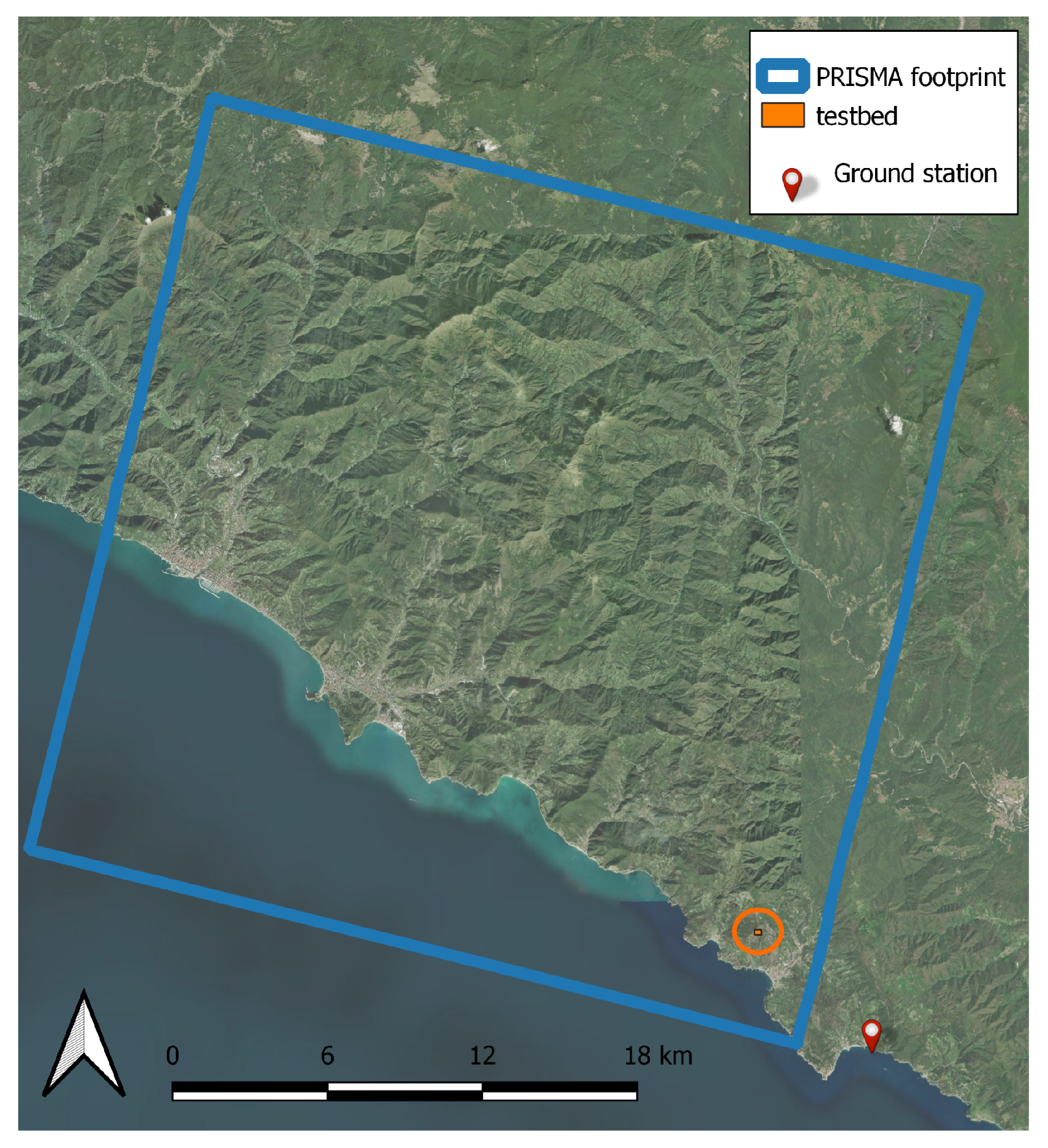
Figure 7.
Geographic extent of the second testbed (Monterosso, in Northern Italy), highlighting PRISMA coverage (tilted blue square), the chosen testbed area simultaneously acquired by both Sentinel-1 and PRISMA (small orange square in an orange circle at the bottom-right corner of the PRISMA coverage) and the ground-truth station (red dot at the bottom-right corner of the Figure, outside the PRISMA coverage area).
The ground station provided extensive time series of the VWC in Monterosso from 2021 to 2023 [48]. On August 25th, 2022, both PRISMA and Sentinel-1 acquired satellite data simultaneously, only 6 km away from the ground station (see Methods). This acquisition took place seven days after a very heavy rainfall lasting several hours, which followed a dry period of approximately three weeks in the summer of 2022 [48], a weather pattern that could potentially lead to landslide triggering. We therefore collected and analysed the satellite data and the VWC from the four soil moisture sensors available at the ground station. The station is installed on terrain of the same type, with scarce vegetation and mineral composition extremely similar to that of the testbed (see Methods). The station provides ground VWC data every 5 minutes and we averaged 10 values around the nominal time of satellite acquisition (August 25th 2022, 10.30 a.m.). Two sensors were positioned 50 cm below ground level (b.g.l.) and two other sensors were at 80 cm b.g.l. Table 1 below shows that the ground sensors provide a “range” of VWC values ranging from to with no correlation with depth, which is not surprising given that these are point measurements of the VWC in a particular soil location a few cubic centimeters. The time series of the four ground sensors in the day of the acquisition look very similar and they can be made to coincide with a proportionality factor. Satellite sensors, on the other hand, provide VWC values integrated over a much larger area, even for the individual pixel ( m2 for Sentinel-1, or m2 for PRISMA), however, they do not show time series information. In the table below we report the VWC data for the four ground sensors, for three locations with scarce vegetation cover selected among the PRISMA image pixels, and for five Sentinel-1 pixels overlapping with the PRISMA pixels. The method of calculation of the VWC from satellite data was the same as reported above.
Table 1 also reports the maximum variability for each dataset (difference between maximum and minimum VWC measured with the same sensor at the same time at nearby locations) and the average among all measured VWC values of each dataset. Looking at Table 1, one can conclude that the variability of VWC data is high (around for ground sensors, and around for satellite sensors), so high in the case of PRISMA as to include the entire variability range of the ground sensors. This fact corroborates the agreement among the different sensors, but it also points out the difficulty of determining a single, precise value of VWC at a given time and location, with any technique, or suite of techniques. The variability of the SAR data is similar to that of the PRISMA data, although there is no obvious correspondence among Sentinel-1 pixel values and PRISMA pixel values in this case. One may notice that the VWC values obtained with the SAR technique are consistently higher by than those obtained with the hyperspectral and ground techniques. It seems therefore, that the SAR data require an absolute calibration procedure, which is almost not needed for the hyperspectral data (assuming the average of the ground sensors as the absolute calibration value). This point will be discussed below.
5. Discussion
The results detailed in the previous section show that hyperspectral and active SAR satellite products can be used to detect soil moisture with a spatial resolution of tens of meters. This is much better than the resolution provided by passive microwave radiometers of approximately km2, which is considered the state of the art for space-borne soil moisture mapping used in global environmental science and in agriculture. The spatial resolution of PRISMA of m2 appears to be more than sufficient for mapping canyons, riverbeds, hill slopes and other local geomorphological structures that may be related to hydrogeological hazard. Satellite imaging of the soil moisture is therefore well positioned to become a key tool for hydrogeological risk monitoring.
The range of VWC values accessible with our SAR and hyperspectral algorithms is approximately . This range certainly allows the monitoring of critical thresholds for hydrogeological risk monitoring, typically set in the range . By close comparison of the absolute VWC values of SAR, hyperspectral and ground sensor data used in this study, however, an intrinsic difficulty has emerged in determining a single, precise value of VWC at a given time and location, with any technique. The satellite measurements provide reliable mapping of the soil moisture at a given time, or at several times separated by many days or months, after which the same satellite passes again on the same location. The ground sensors provide reliable time series with high temporal resolution of a few minutes, but cannot cover large areas and can hardly provide full VWC maps of geomorphological structures related to hydrogeological hazard. In other words, a combination of ground and satellite data seems to be required in the future to build a risk monitoring network operating as a semi-automated alarm system.
The determination of the VWC from SAR or hyperspectral satellite data becomes considerably more difficult in the presence of dense vegetation cover. SAR cross sections are heavily impacted by vegetation, and SWIR radiation cannot be transmitted at all through thick leaf coverage. In our analysis, we have purposely chosen a vegetation-free testbed in Southern Italy to demonstrate the physical principle, but we have encountered considerable difficulties when moving to a more vegetated area (Monterosso) for the calibration with ground sensors. In this respect, there is an inherent advantage in hyperspectral imaging compared to SAR: the possibility of discarding pixels with too high vegetation cover that are directly identified from the red edge of chlorophyll at 800 nm in the hyperspectral data, without the need of image co-registration with other satellite images or map databases.
Finally, the consistency of the SAR and hyperspectral datasets can be demonstrated by calculating the Pearson’s correlation coefficient among two selected sub-datasets where no vegetation cover, or slope angle, or surface roughness issues have emerged. The sub-datasets have been identified in the bottom-left corner of the maps in Figure 6. Figure 8 shows the Pearson’s correlation plot of all pixels contained in the red rectangular contour of the two maps, SAR and hyperspectral. One can immediately see a positive correlation buildup, although far from identity. Also, a calibration issue emerges: the range of the SAR sub-dataset is higher by than the range of the hyperspectral dataset. This corresponds to the observation made in Table 1, which is related to a different testbed (Monterosso), where the SAR VWC are higher than both the hyperspectral and ground VWCs by approximately . We therefore used the Pearson’s plot in Figure 8 to calculate the best-fit calibration coefficient for the absolute VWC values obtained with the SAR technique: we assumed that the Pearson’s correlation coefficient would be exactly 1 if there were no deviations (i.e. that the two satellite techniques measure the same physical observable), and we have found that dividing all the SAR VWC values by a phenomenological calibration parameter validates this assumption. This is highlighted in the corrected Pearson’s plot of Figure 9, which shows an almost perfect diagonal distribution with VWC range between and . Possible explanations of this parameter reside in the assumptions made in the SAR scattering cross-section model [47], which have a strong dependence on the observation angle, and in the lack of a well-controlled reference pixel in the SAR images. In the hyperspectral images, the use of a flat metallic or rocky surface as the reference pixel in the same image, used to calculate the absolute reflectivity from the raw reflectance data, eliminates this issue. Interestingly, the parameter determined from the Southern Italy testbed also corrects the SAR data in Table 1 from the Monterosso testbed, aligning them with hyperspectral and ground sensor data (see Table 1), therefore it may be specific to the chosen SAR cross-section model.
After the phenomenological calibration, the calculation of the Pearson’s correlation coefficient between SAR and hyperspectral data gives , which demonstrates the existence of a positive correlation, although in the presence of heavy disturbances, even in the selected vegetation-free area in Southern Italy. The remaining disturbances may be due to different mineral composition (which mainly impacts the hyperspectral data), surface roughness (mainly impacting the SAR data), local variations of the angle of incidence (impacting both), and co-registration errors, among others.
6. Conclusions
In this work, we demonstrated hydrogeological hazard monitoring (landslide risk triggered by soil moisture) through the analysis of satellite data to retrieve the local soil moisture. Volumetric water content maps with values in the range have been calculated from hyperspectral SWIR and active SAR data collected on the same testbed at nearly the same time and successfully compared. A calibration procedure with ground-based soil moisture sensors was also performed in a different testbed, highlighting the difficulty of obtaining a compatible value of the VWC with different techniques. A positive correlation between SAR and hyperspectral soil moisture data has been obtained.
Our results demonstrate that hyperspectral monitoring of the soil moisture from satellites is possible with high accuracy and spatial resolutions of the order of tens of meters, which is sufficient for hydrogeological risk monitoring. Satellite revisit times will be defined by future hyperspectral missions, but they are expected to be of few days or less. These parameters look promising for the development of a quasi-real time hydrogeological risk monitoring tool and semi-automated alarm system based on the data fusion of radar and hyperspectral satellite imaging.
Author Contributions
Conceptualization, M.O. and V.G.; methodology, M.O.; software, A.P., A.M., C.M., K.K. and F.V.; validation, C.E., C.M., K.K., A.P. and A.M.; formal analysis, A.P., V.G. and M.O.; investigation, K.K., A.M. and C.M.; resources, P.M., V.G. and M.O.; data curation, K.K., A.P., C.E. and M.O.; writing—original draft preparation, M.O., A.M. and A.P.; writing—review and editing, M.O. and K.K.; visualization, K.K., A.P. and A.M.; supervision, M.O.; project administration, P.M. and V.G.; funding acquisition, P.M., V.G. and M.O. All authors have read and agreed to the published version of the manuscript.
Funding
This work has been funded by the European Union through the European Regional Development Fund POR FESR Lazio 2021-2027 - Project T0008B0005 - A0613 "NARCISSUS" - CUP F89J23001420007.
Data Availability Statement
The data presented in this study are available on request from the corresponding author.
Conflicts of Interest
The authors declare no conflicts of interest.
References
- Furtak, K.; Wolińska, A. The impact of extreme weather events as a consequence of climate change on the soil moisture and on the quality of the soil environment and agriculture – A review. CATENA 2023, 231, 107378. [Google Scholar] [CrossRef]
- Legates, D.R.; Mahmood, R.; Levia, D.F.; DeLiberty, T.L.; Quiring, S.M.; Houser, C.; Nelson, F.E. Soil moisture: A central and unifying theme in physical geography. Progress in Physical Geography: Earth and Environment 2011, 35, 65–86. [Google Scholar] [CrossRef]
- Seneviratne, S.I.; Corti, T.; Davin, E.L.; Hirschi, M.; Jaeger, E.B.; Lehner, I.; Orlowsky, B.; Teuling, A.J. Investigating soil moisture–climate interactions in a changing climate: A review. Earth-Science Reviews 2010, 99, 125–161. [Google Scholar] [CrossRef]
- Dirmeyer, P.A.; Schlosser, C.A.; Brubaker, K.L. Precipitation, recycling, and land memory: An integrated analysis. Journal of Hydrometeorology 2009, 10, 278–288. [Google Scholar] [CrossRef]
- Oyounalsoud, M.S.; Yilmaz, A.G.; Abdallah, M.; Abdeljaber, A. Drought prediction using artificial intelligence models based on climate data and soil moisture. Scientific Reports 2024, 14, 19700. [Google Scholar] [CrossRef]
- Whiteley, J.S.; Chambers, J.E.; Uhlemann, S.; Wilkinson, P.B.; Kendall, J.M. Geophysical Monitoring of Moisture-Induced Landslides: A Review. Reviews of Geophysics 2019, 57, 106–145, [https://agupubs.onlinelibrary.wiley.com/doi/pdf/10.1029/2018RG000603]. [Google Scholar] [CrossRef]
- Ray, R.L.; Jacobs, J.M. Relationships among remotely sensed soil moisture, precipitation and landslide events. Natural Hazards 2007, 43, 211–222. [Google Scholar] [CrossRef]
- Van Asch, T.; Buma, J.; Van Beek, L. A view on some hydrological triggering systems in landslides. Geomorphology 1999, 30, 25–32. [Google Scholar] [CrossRef]
- Chifflard, P.; Kranl, J.; zur Strassen, G.; Zepp, H. The significance of soil moisture in forecasting characteristics of flood events. A statistical analysis in two nested catchments. Journal of Hydrology and Hydromechanics 2018, 66, 1. [Google Scholar] [CrossRef]
- Kim, S.; Zhang, R.; Pham, H.; Sharma, A. A review of satellite-derived soil moisture and its usage for flood estimation. Remote Sensing in Earth Systems Sciences 2019, 2, 225–246. [Google Scholar] [CrossRef]
- Wang, T.; Singh, S.K.; Bárdossy, A. On the use of the critical event concept for quantifying soil moisture dynamics. Geoderma 2019, 335, 27–34. [Google Scholar] [CrossRef]
- Rosenbaum, U.; Bogena, H.R.; Herbst, M.; Huisman, J.A.; Peterson, T.J.; Weuthen, A.; Western, A.W.; Vereecken, H. Seasonal and event dynamics of spatial soil moisture patterns at the small catchment scale. Water Resources Research 2012, 48. [https://agupubs.onlinelibrary.wiley.com/doi/pdf/10.1029/2011WR011518]. [Google Scholar] [CrossRef]
- Rasheed, M.W.; Tang, J.; Sarwar, A.; Shah, S.; Saddique, N.; Khan, M.U.; Imran Khan, M.; Nawaz, S.; Shamshiri, R.R.; Aziz, M.; et al. Soil Moisture Measuring Techniques and Factors Affecting the Moisture Dynamics: A Comprehensive Review. Sustainability 2022, 14. [Google Scholar] [CrossRef]
- Brocca, L.; Ciabatta, L.; Massari, C.; Camici, S.; Tarpanelli, A. Soil Moisture for Hydrological Applications: Open Questions and New Opportunities. Water 2017, 9. [Google Scholar] [CrossRef]
- Galeazzi, C.; Sacchetti, A.; Cisbani, A.; Babini, G. The PRISMA program. In Proceedings of the IGARSS 2008-2008 IEEE International Geoscience and Remote Sensing Symposium. IEEE, 2008, Vol. 4, pp. IV–105.
- European Space Agency. Sentinel-1: Mission and Ground Segment. ESA Special Publication SP-1322/1, ESA Communications, 2009. Accessed June 2025. 20 June.
- Xie, Q.; Menenti, M.; Jia, L. Improving the AMSR-E/NASA soil moisture data product using in-situ measurements from the Tibetan Plateau. Remote Sensing 2019, 11, 2748. [Google Scholar] [CrossRef]
- NASA Jet Propulsion Laboratory. SMAP Mission Description, 2015. Online mission overview; describes mission goals, launch, instruments, and orbit.
- Paloscia, S.; Pettinato, S.; Santi, E.; Notarnicola, C.; Pasolli, L.; Reppucci, A. Soil moisture mapping using Sentinel-1 images: Algorithm and preliminary validation. Remote Sensing of Environment 2013, 134, 234. [Google Scholar] [CrossRef]
- Profeti, G.; Macintosh, H. Flood management through Landsat TM and ERS SAR data: a case study. Hydrological Processes 1997, 11, 1397–1408. [Google Scholar] [CrossRef]
- Vicente-Serrano, S.M.; Pons-Fernández, X.; Cuadrat-Prats, J. Mapping soil moisture in the central Ebro river valley (northeast Spain) with Landsat and NOAA satellite imagery: a comparison with meteorological data. International Journal of Remote Sensing 2004, 25, 4325–4350. [Google Scholar] [CrossRef]
- Zhang, Y.; Wegehenkel, M. Integration of MODIS data into a simple model for the spatial distributed simulation of soil water content and evapotranspiration. Remote sensing of Environment 2006, 104, 393–408. [Google Scholar] [CrossRef]
- Liu, S.F.; Liou, Y.A.; Wang, W.J.; Wigneron, J.P.; Lee, J.B. Retrieval of crop biomass and soil moisture from measured 1.4 and 10.65 GHz brightness temperatures. IEEE Transactions on Geoscience and Remote Sensing 2002, 40, 1260–1268. [Google Scholar]
- Sadeghi, M.; Jones, S.B.; Philpot, W.D. A linear physically-based model for remote sensing of soil moisture using short wave infrared bands. Remote Sensing of Environment 2015, 164, 66–76. [Google Scholar] [CrossRef]
- Weidong, L.; Baret, F.; Xingfa, G.; Qingxi, T.; Lanfen, Z.; Bing, Z. Relating soil surface moisture to reflectance. Remote sensing of environment 2002, 81, 238–246. [Google Scholar] [CrossRef]
- Kruse, F.; Boardman, J.; Huntington, J. Comparison of airborne hyperspectral data and EO-1 Hyperion for mineral mapping. IEEE Transactions on Geoscience and Remote Sensing 2003, 41, 1388–1400. [Google Scholar] [CrossRef]
- Song, X.; Ma, J.; Li, X.; Leng, P.; Zhou, F.; Li, S. First results of estimating surface soil moisture in the vegetated areas using ASAR and Hyperion data: The Chinese Heihe River Basin Case Study. Remote Sensing 2014, 6, 12055–12069. [Google Scholar] [CrossRef]
- Babaeian, E.; Sadeghi, M.; Jones, S.B.; Montzka, C.; Vereecken, H.; Tuller, M. Ground, Proximal, and Satellite Remote Sensing of Soil Moisture. Reviews of Geophysics 2019, 57, 530–616, [https://agupubs.onlinelibrary.wiley.com/doi/pdf/10.1029/2018RG000618]. [Google Scholar] [CrossRef]
- Pierdicca, N.; Pulvirenti, L.; Pace, G. A Prototype Software Package to Retrieve Soil Moisture From Sentinel-1 Data by Using a Bayesian Multitemporal Algorithm. IEEE Journal of Selected Topics in Applied Earth Observations and Remote Sensing 2014, 7, 153–166. [Google Scholar] [CrossRef]
- Bhosle, K.; Musande, V. Evaluation of Deep Learning CNN Model for Land Use Land Cover Classification and Crop Identification Using Hyperspectral Remote Sensing Images. Journal of the Indian Society of Remote Sensing 2019, 47, 1949–1958. [Google Scholar] [CrossRef]
- Xu, B.; Gong, P. Land-use/Land-cover Classification with Multispectral and Hyperspectral EO-1 Data. Photogrammetric Engineering & Remote Sensing 2007, 73, 955–965. [Google Scholar] [CrossRef]
- Cai, X.; Wu, L.; Li, Y.; Lei, S.; Xu, J.; Lyu, H.; Li, J.; Wang, H.; Dong, X.; Zhu, Y.; et al. Remote sensing identification of urban water pollution source types using hyperspectral data. Journal of Hazardous Materials 2023, 459, 132080. [Google Scholar] [CrossRef]
- Arellano, P.; Tansey, K.; Balzter, H.; Boyd, D.S. Detecting the effects of hydrocarbon pollution in the Amazon forest using hyperspectral satellite images. Environmental Pollution 2015, 205, 225–239. [Google Scholar] [CrossRef]
- Katlane, R.; Doxaran, D.; ElKilani, B.; Trabelsi, C. Remote sensing of turbidity in optically shallow waters using sentinel-2 MSI and PRISMA satellite data. PFG–Journal of Photogrammetry, Remote Sensing and Geoinformation Science 2024, 92, 431–447. [Google Scholar] [CrossRef]
- Lazzeri, G.; Frodella, W.; Rossi, G.; Moretti, S. Multitemporal mapping of post-fire land cover using multiplatform PRISMA hyperspectral and Sentinel-UAV multispectral data: Insights from case studies in Portugal and Italy. Sensors 2021, 21, 3982. [Google Scholar] [CrossRef]
- Bedini, E.; Chen, J. Application of PRISMA satellite hyperspectral imagery to mineral alteration mapping at Cuprite, Nevada, USA. Journal of hyperspectral remote sensing 2020, 10, 87–94. [Google Scholar] [CrossRef]
- Tian, J.; Philpot, W.D. Relationship between surface soil water content, evaporation rate, and water absorption band depths in SWIR reflectance spectra. Remote Sensing of Environment 2015, 169, 280–289. [Google Scholar] [CrossRef]
- Philpot, W. Spectral reflectance of wetted soils. Proceedings of ASD and IEEE GRS 2010, 2, 1–12. [Google Scholar]
- Lobell, D.B.; Di Tommaso, S.; Burney, J.A. Globally ubiquitous negative effects of nitrogen dioxide on crop growth. Science Advances 2022, 8, eabm9909. [Google Scholar] [CrossRef]
- Camerini, M.; Mancini, M.; Fossati, E.; Battazza, F.; Formaro, R. The PRISMA hyperspectral imaging spectrometer: detectors and front-end electronics. SPIE 2013. [Google Scholar] [CrossRef]
- Destefanis, G.; Tribolet, P. Advanced MCT technologies in France. In Proceedings of the Infrared Technology and Applications XXXIII; Andresen, B.F.; Fulop, G.F.; Norton, P.R., Eds. International Society for Optics and Photonics, SPIE, 2007, Vol. 6542, p. 65420D.
- Cogliati, S.; Sarti, F.; Chiarantini, L.; Cosi, M.; Lorusso, R.; Lopinto, E.; Miglietta, F.; Genesio, L.; Guanter, L.; Damm, A.; et al. The PRISMA imaging spectroscopy mission: overview and first performance analysis. Remote Sensing of Environment 2021, 262, 112499. [Google Scholar] [CrossRef]
- Labate, D.; Ceccherini, M.; Cisbani, A.; De Cosmo, V.; Galeazzi, C.; Giunti, L.; Melozzi, M.; Pieraccini, S.; Stagi, M. The PRISMA payload optomechanical design, a high performance instrument for a new hyperspectral mission. Acta Astronautica 2009, 65, 1429–1436. [Google Scholar] [CrossRef]
- Pierdicca, N.; Pulvirenti, L.; Bignami, C. Soil moisture estimation over vegetated terrains using multitemporal remote sensing data. Remote Sensing of Environment 2010, 114, 440–448. [Google Scholar] [CrossRef]
- Arabini, E.; Patacchini, A.; Anconitano, G.; Pierdicca, N.; et al. ROSE-L and Sentinel-1 soil moisture retrieval: a simulated study. In Proceedings of the IGARSS 2024-2024 IEEE International Geoscience and Remote Sensing Symposium, 2024.
- Dobson, M.; Ulaby, F.; Hallikainen, M.; El-Rayes, M. Microwave Dielectric Behavior of Wet Soil-Part II: Dielectric Mixing Models. Geoscience and Remote Sensing, IEEE Transactions on 1985, GE-23, 35–46. [Google Scholar] [CrossRef]
- Oh, Y.; Sarabandi, K.; Ulaby, F.T. An empirical model and an inversion technique for radar scattering from bare soil surfaces. IEEE transactions on Geoscience and Remote Sensing 2002, 30, 370–381. [Google Scholar] [CrossRef]
- Fiorucci, M.; Pepe, G.; Marmoni, G.M.; Pecci, M.; Di Martire, D.; Guerriero, L.; Bausilio, G.; Vitale, E.; Raso, E.; Raimondi, L.; et al. Long-term hydrological monitoring of soils in the terraced environment of Cinque Terre (north-western Italy). Frontiers in Earth Science 2023, 11, 1285669. [Google Scholar] [CrossRef]
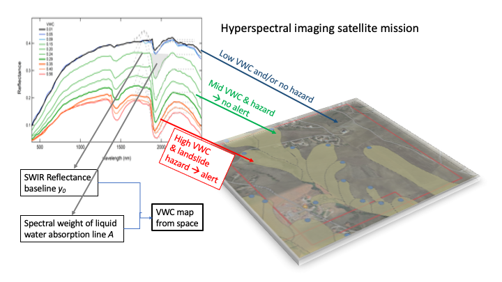
Figure 1.
Concept of the work. Hyperspectral and SAR images are analyzed with physics-informed models to obtain a reliable value of soil moisture (VWC) per each pixel. The two soil moisture maps are compared and cross-validated, and super-imposed to maps of known hydrogeological risk areas. In case a quasi-real-time data analysis protocol can be developed in the future, alerts for hydrogeological risk may be launched directly from satellites.
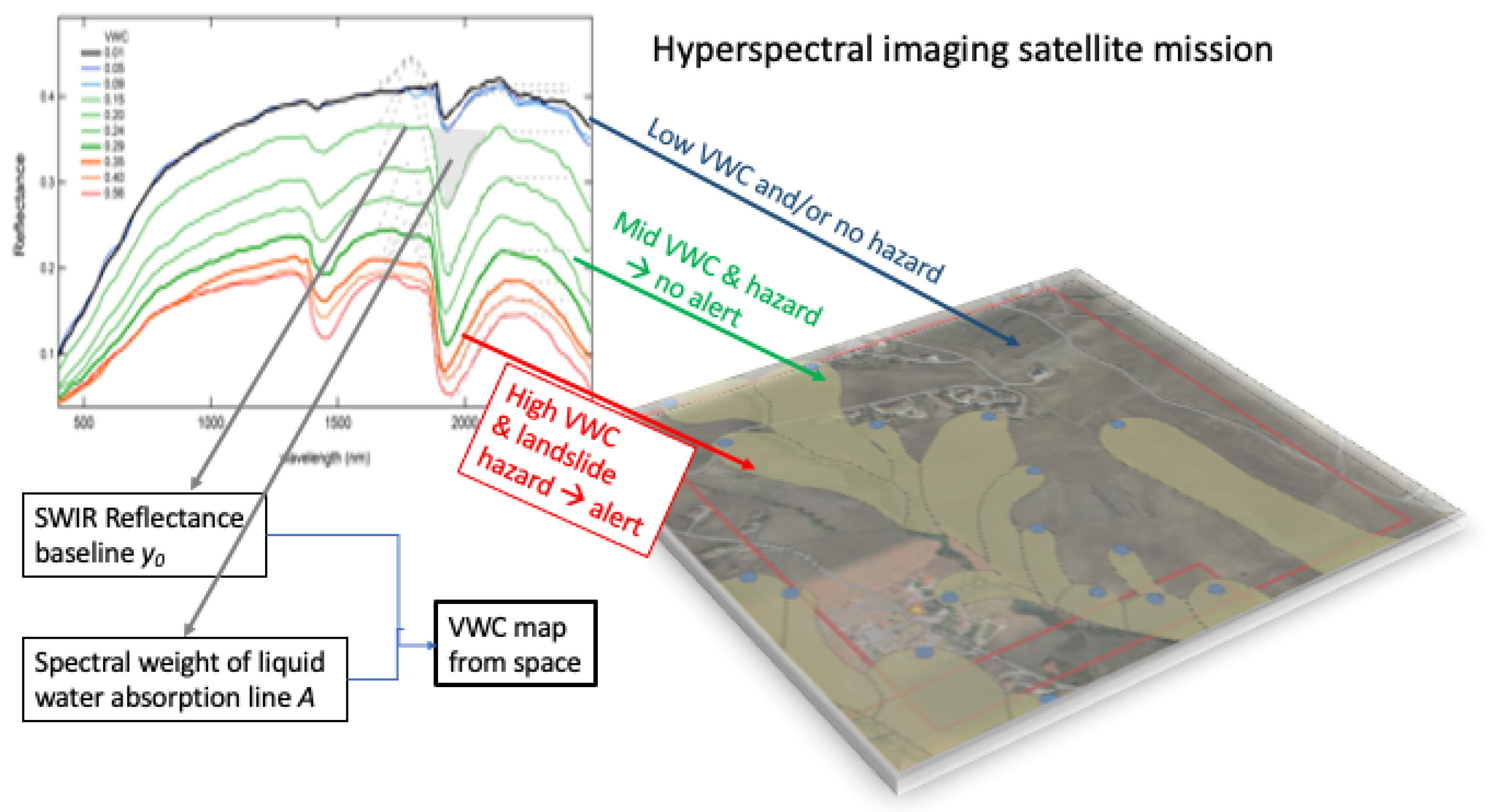
Figure 2.
Examples of two PRISMA spectra, top panel with low VWC and bottom panel with high VWC. The fit based on the Weibull function is also shown (thick curve).
Figure 2.
Examples of two PRISMA spectra, top panel with low VWC and bottom panel with high VWC. The fit based on the Weibull function is also shown (thick curve).
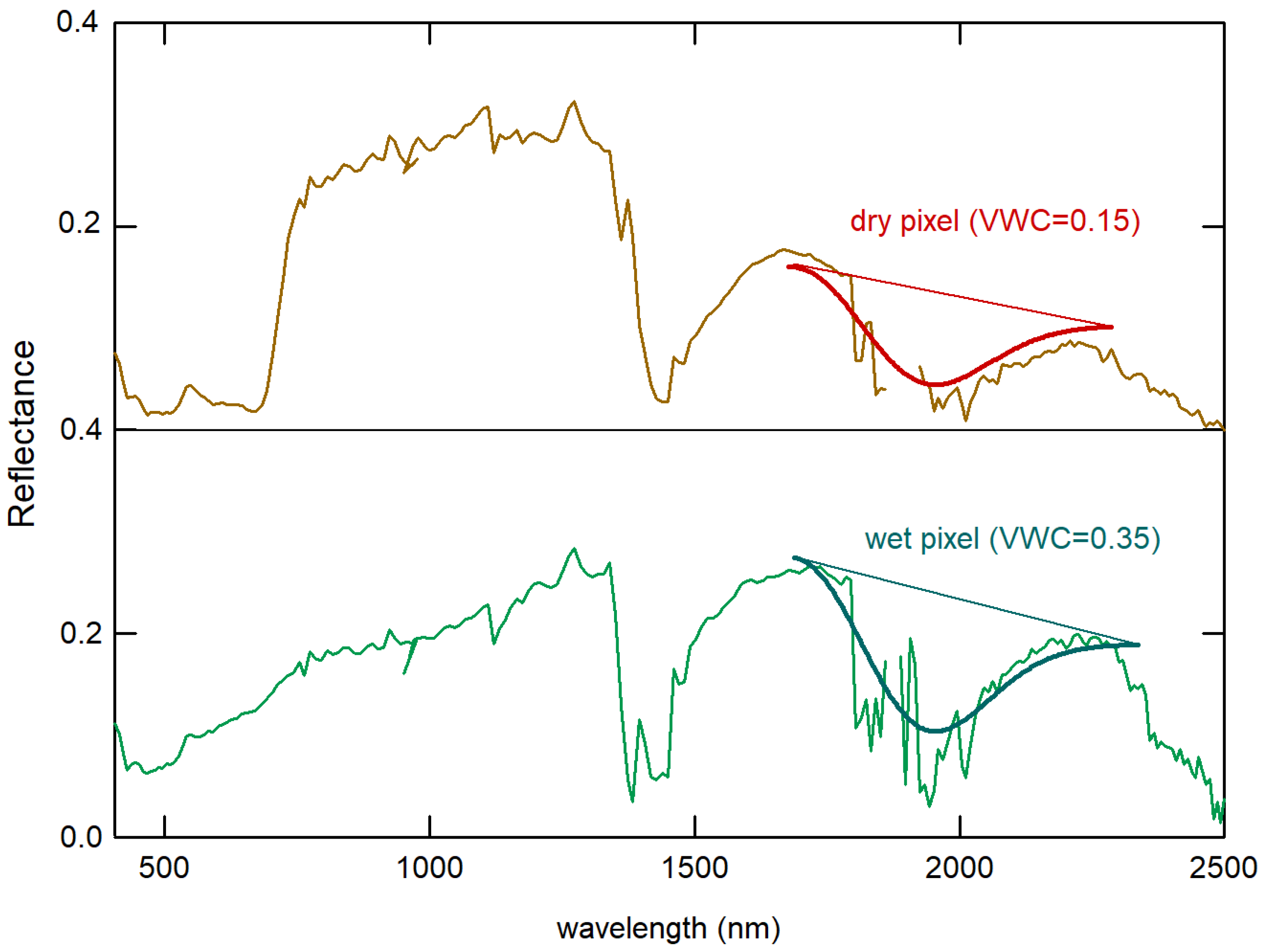
Figure 3.
XY Rasters of the fitting parameters A and obtained from the PRISMA hypercube, and raster of the calculated soil moisture in terms of VWC.
Figure 3.
XY Rasters of the fitting parameters A and obtained from the PRISMA hypercube, and raster of the calculated soil moisture in terms of VWC.
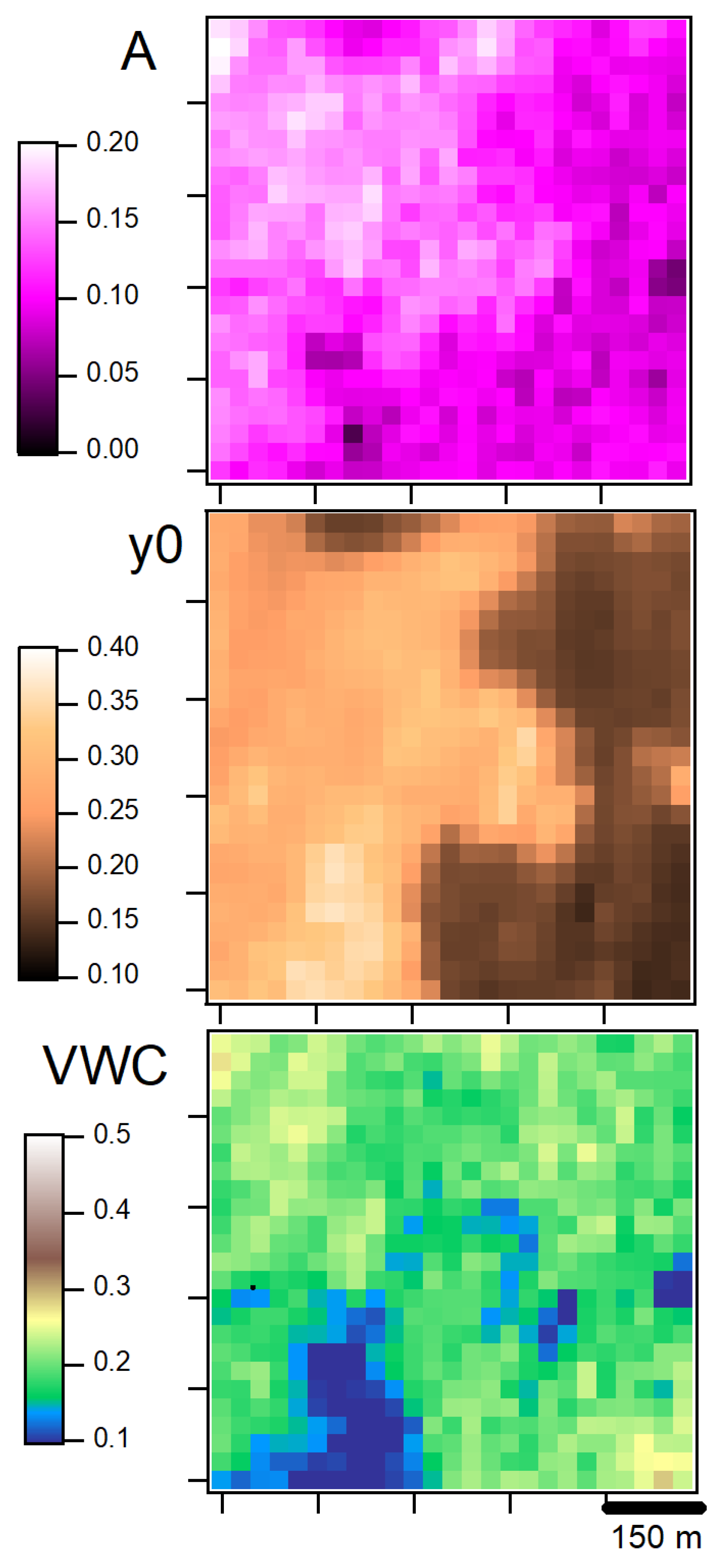
Figure 4.
SAR data analysis workflow for processing raw satellite Sentinel-1 images. After reading the data, a thermal noise removal algorithm is applied to enhance signal quality. Positional inaccuracies are corrected with the application of the orbit file, followed by GRD border noise removal. Calibration is performed to convert pixel values into backscatter coefficients, after which speckle filter is applied to reduce the noise appearing as a random pattern on diffusion surface elements. Using a digital elevation model we apply terrain correction for topographic distortions, and finally collocation to align the images spatially. A subset of the image is derived accounting for the area of interest.
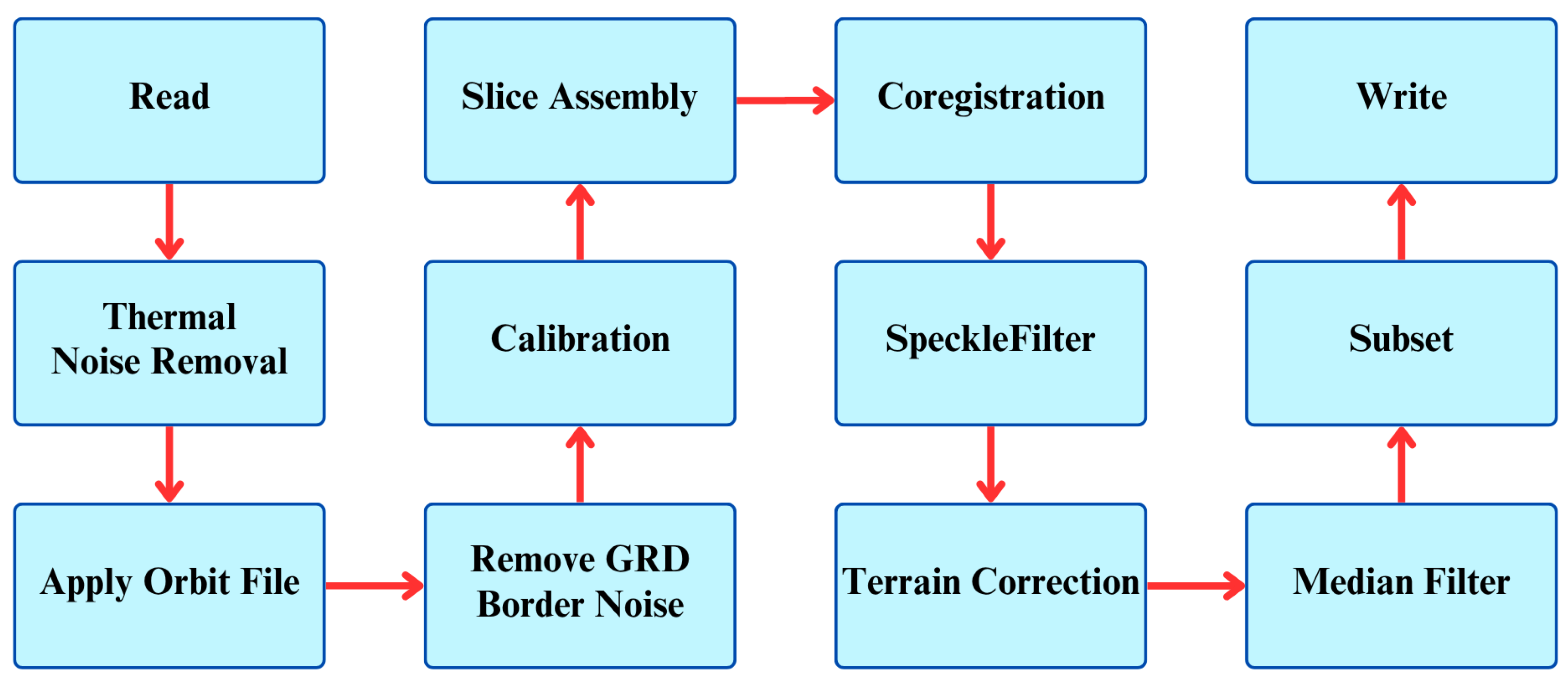
Figure 5.
Testbed located in Southern Italy (Picerno, Basilicata region). The bounding box in GPS coordinates is: lower left corner , lower right corner upper left corner upper right corner .
Figure 5.
Testbed located in Southern Italy (Picerno, Basilicata region). The bounding box in GPS coordinates is: lower left corner , lower right corner upper left corner upper right corner .
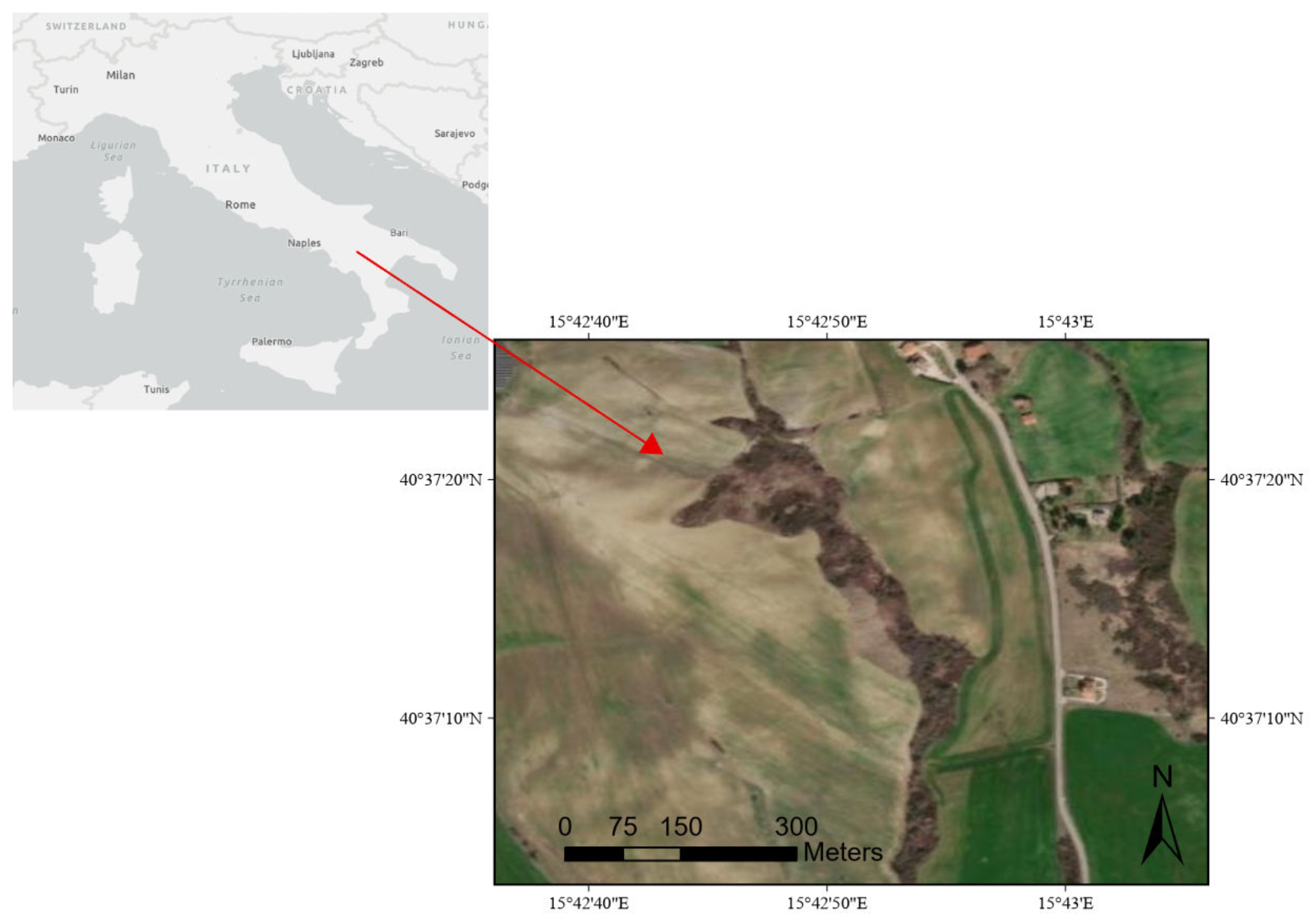
Figure 6.
Multi-source observation of the test area for landslide. (a) Topography showing mapped landslide features. (b) soil moisture level extracted from Sentinel-1 SAR image. (c) PRISMA image showing water content. Data in both (b) and (c) have been expressed as VWC for comparison. Note that there is an apparent X-offset of approximately 120 m between the (0,0) point of maps (b) and of map (c), of unknown origin.
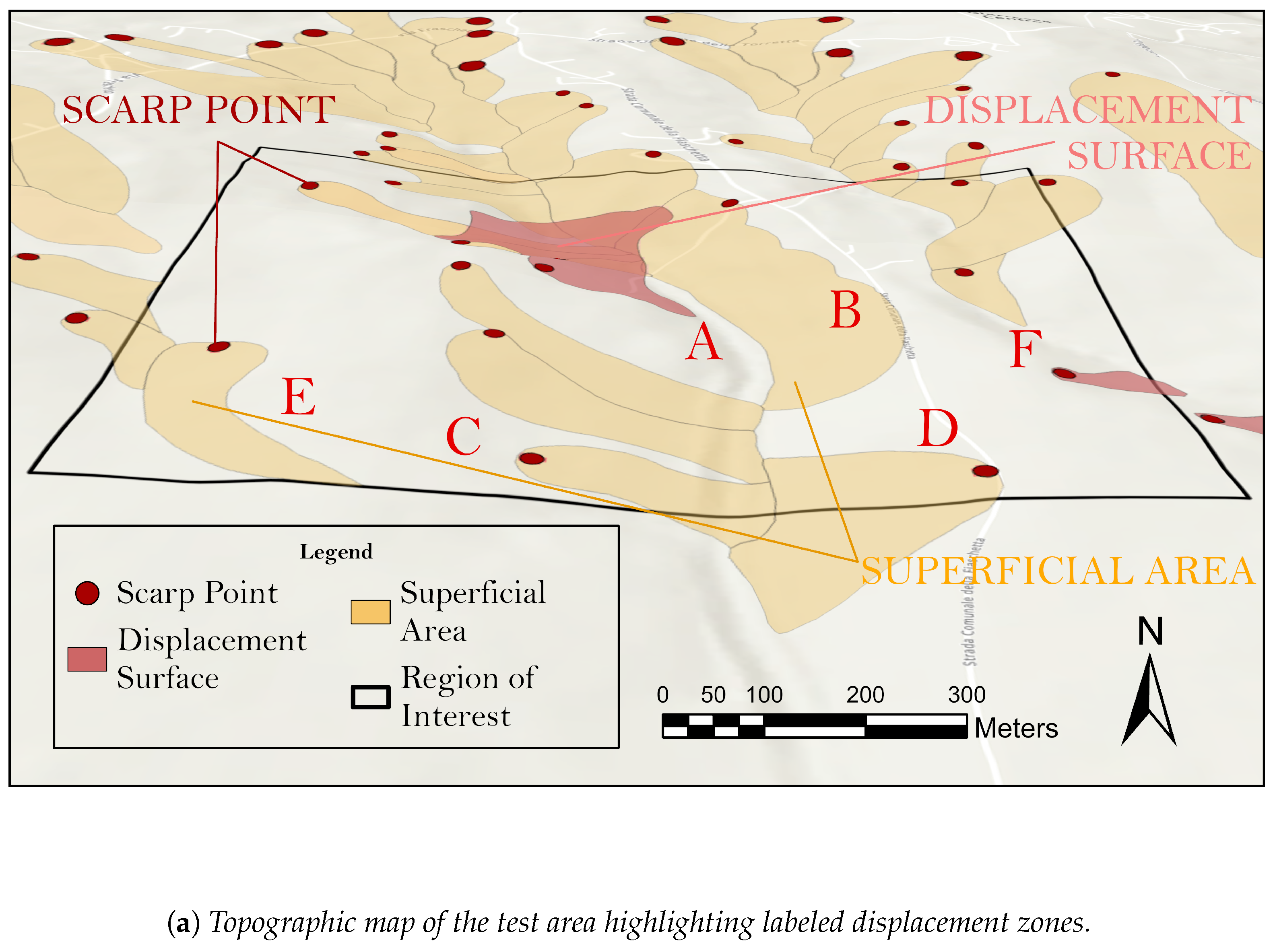
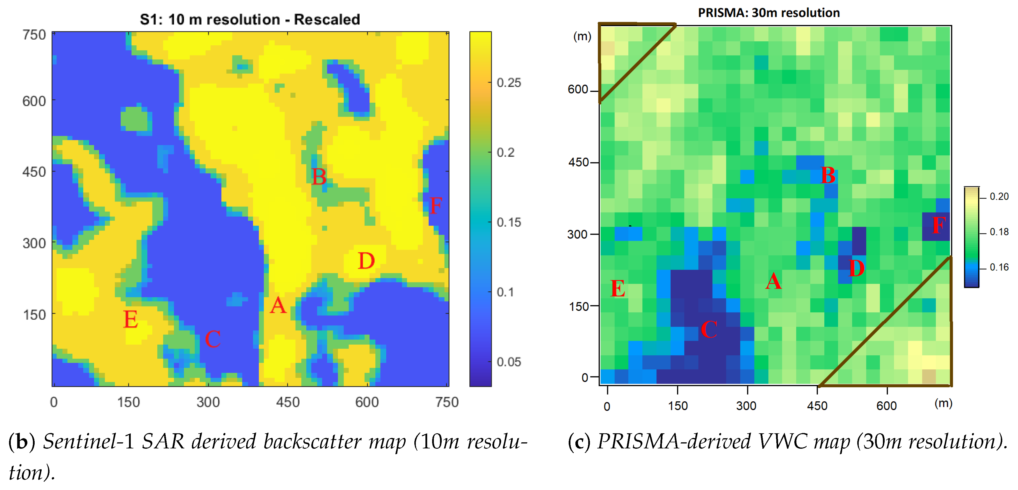
Figure 8.
Raw correlation plot of the SAR and hyperspectral pixels taken from a selected subset of pixels in the VWC maps indicated by the red rectangular contour in the insets, showing the two VWC maps in Figure 6 in grayscale.
Figure 8.
Raw correlation plot of the SAR and hyperspectral pixels taken from a selected subset of pixels in the VWC maps indicated by the red rectangular contour in the insets, showing the two VWC maps in Figure 6 in grayscale.
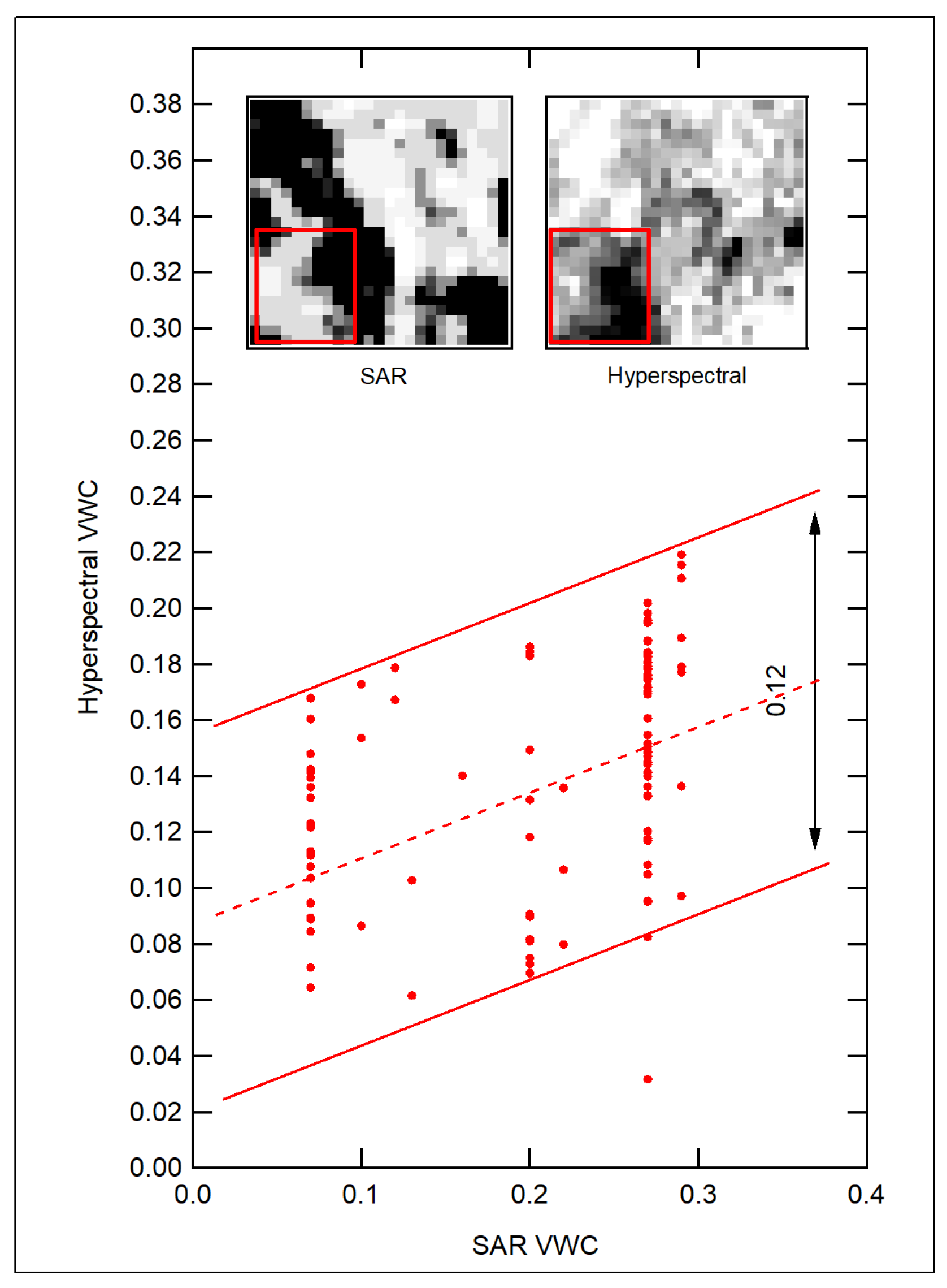
Figure 9.
Pearson’s correlation plot of the SAR and hyperspectral pixels of Figure 8, with the SAR VWC values divided by a phenomenological calibration parameter .
Figure 9.
Pearson’s correlation plot of the SAR and hyperspectral pixels of Figure 8, with the SAR VWC values divided by a phenomenological calibration parameter .
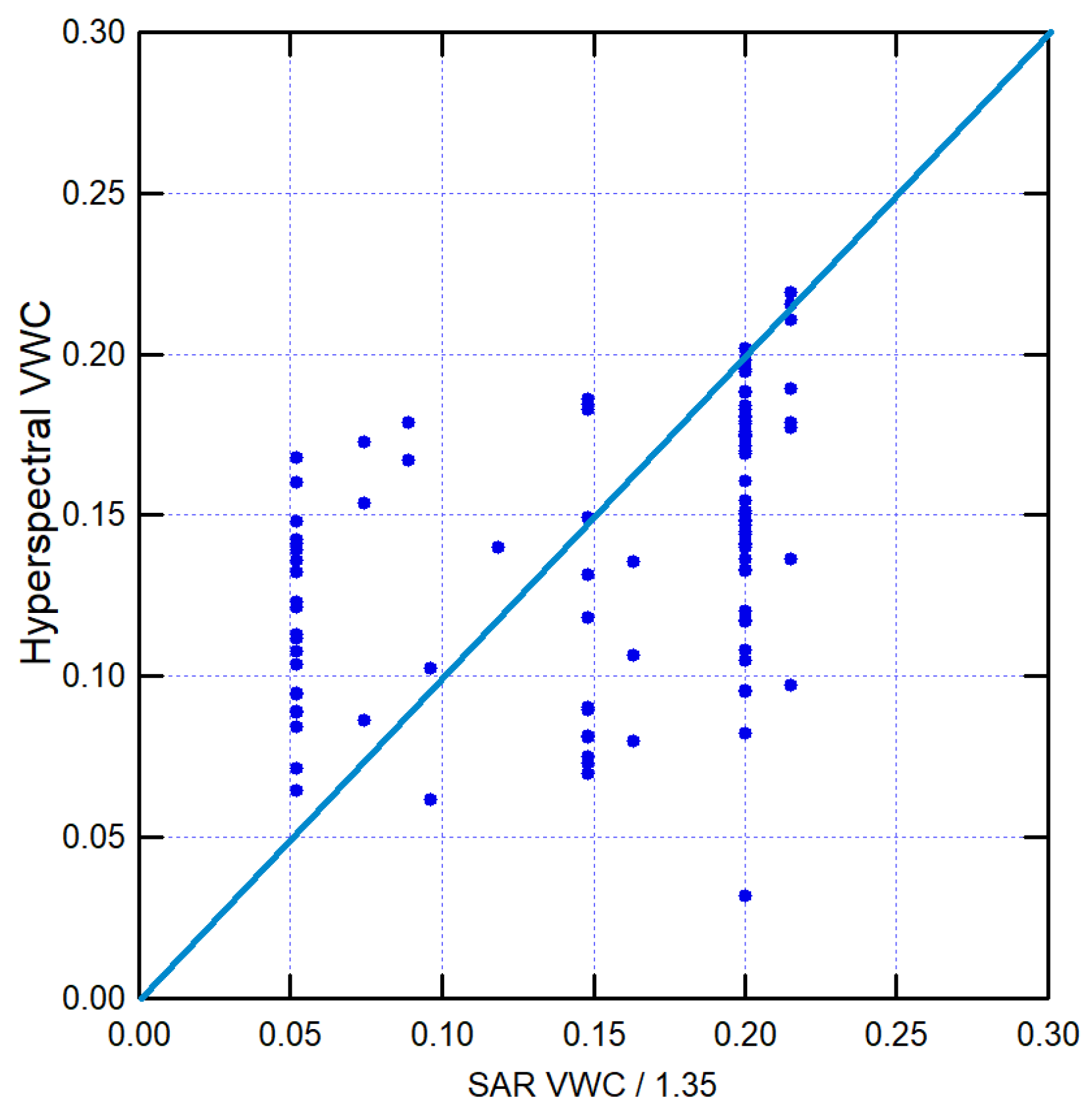

Table 1.
Volumetric water content at the testbed "Monterosso" on August 24th, 2022, measured with ground sensors and with the two satellite methods. VWC values in the first column are for all available probes and pixels in the testbed, in the second column we report the variability range of each technique and in the third column the average.
| Sensor | VWC all | VWC max-min | VWC avg |
|---|---|---|---|
| Ground - permittivity | 0.159 | ||
| 0.173 | 0.053 | 0.18 | |
| 0.169 | |||
| 0.212 | |||
| PRISMA - hyperspectral | 0.196 | ||
| 0.250 | 0.099 | 0.20 | |
| 0.151 | |||
| Sentinel 1 - SAR | 0.28 | ||
| 0.35 | |||
| 0.28 | 0.09 | 0.29 | |
| 0.35 | |||
| 0.26 |
Disclaimer/Publisher’s Note: The statements, opinions and data contained in all publications are solely those of the individual author(s) and contributor(s) and not of MDPI and/or the editor(s). MDPI and/or the editor(s) disclaim responsibility for any injury to people or property resulting from any ideas, methods, instructions or products referred to in the content. |
© 2025 by the authors. Licensee MDPI, Basel, Switzerland. This article is an open access article distributed under the terms and conditions of the Creative Commons Attribution (CC BY) license (http://creativecommons.org/licenses/by/4.0/).
Copyright: This open access article is published under a Creative Commons CC BY 4.0 license, which permit the free download, distribution, and reuse, provided that the author and preprint are cited in any reuse.


