
Submitted:
02 December 2025
Posted:
03 December 2025
You are already at the latest version
Abstract
This paper investigates a delayed reaction-diffusion-advection population model that incorporates delay and strong Allee effect. Firstly, the effect of the advection rate on the stability of constant steady state within the model is examined. Analysis indicates that under the given conditions, larger advection rate can stabilize the constant steady state. Then, the existence of Hopf bifurcations is studied by adopting delay as the varying parameter. Besides, the normal form in the vicinity of the Hopf singularity on the center manifold is calculated by adopting a weighted inner product. Simulations are conducted to validate the theoretical findings. Research shows that under certain conditions, there exists a sequence of bifurcation singularities in the system.
Keywords:
Allee effect
; reaction-diffusion-advection
; normal form
; Hopf bifurcation
1. Introduction
In ecosystems, the logistic growth rate is commonly used to describe population growth, effectively capturing the effect of intraspecific competition. The logistic growth rate describes the fact that when population density increases, the growth rate declines. In 1931, the ecologist Allee observed that in social populations, the intrinsic growth rate decreases below a critical population threshold [1]. This phenomenon, known as the Allee effect, has since been extensively studied in subsequent ecological models [2,3,4].
The Allee effect describes the phenomenon of individual animals benefiting from the presence of conspecifics. The Allee effect is categorized into two types: strong and weak [5,6]. In comparison, models with strong Allee effect exhbit richer properties. The classic strong Allee effect model is as follows:
where is the Allee threshold, K is the carrying capacity of the population. A model incorporating strong Allee effect exhibits a growth rate influenced by cooperative and competitive interactions among individuals. Reference [7] provides numerical evidence that the strong Allee effect is characterized by a critical density threshold, below which population density is insufficient for long-term persistence.
Time delays are ubiquitous in the study of population dynamics [8,9,10]. For example, the birth of new individuals involves a gestation delay, the predation is followed by a digestion delay. Notably, the current population growth rate is determined by environmental pressure, which is governed by the population density times ago. This is a common and widespread phenomenon among social animals.
We should emphasize that in the study of population dynamics within bounded domains, it has been observed that population density varies with spatial location. Individuals undergo both random dispersal and directed movement [12,13]. The diffusion and advection enables the investigation of the spatiotemporal population distribution [11]. Based on these considerations, this paper investigates the following model subject to bounded region and the following boundary conditions:
where denotes the density of the population at the location x and the time t, d () denotes the diffusion rate, () denotes the advection rate, the parameter () represents the carrying capacity, the Allee threshold is rescaled to 1, L () denotes the region range and () represents the time-delayed effect of intraspecific competition on population growth. The boundary conditions are the modified No-flux/Hostile (NF/H) boundary conditions [14], these boundary conditions are commonly used in studying the distribution and migration of species in rivers.
In ecological systems, the stability and periodic oscillation of population sizes are crucial for the long-term persistence of populations. Bifurcation analysis is one of the classical methods for studying population oscillations, and numerous scholars have conducted relevant research in this field [15,16,17,18]. However, studies on the bifurcation theory of population models with advection and diffusion are relatively scarce. Most existing studies focus on abstract theoretical frameworks, and few have performed specific calculations of normal forms.
Recently, several studies have focused on the dynamics of advection-diffusion models [19,20]. Numerical evidence is provided for the occurrence of Hopf bifurcation in a competition model with diffusion and advection [19]. A rigorous analysis of spatially nonhomogeneous equilibrium solutions for a reaction-diffusion-advection model that evolves with nonlocal delay and nonlinear boundary conditions is presented in [20]. Unlike existing studies, this paper aims to theoretically investigate the Hopf bifurcation in the advection-diffusion model (1) and derive the normal form that determines the characteristics of the bifurcation.
Various analytical approaches are available for the study of advection-diffusion models. In our work, we draw support from the operator theory, observe that the eigenfunctions of the linear operator under consideration fail to form an orthogonal basis under the inner product. However, these eigenfunctions become orthogonal by introducing a suitably defined weighted inner product. We emphasize two points of this work: for one thing, we compute the normal forms in a delayed advection-diffusion model with a weighted inner product; for the other, Hopf bifurcation is proved both theoretically and numerically. Besides, the derivation of the normal form here can be extended to other advection-diffusion models with Robin boundary conditions.
The structure of this paper is as follows. Section 2 examines the stability of the positive steady state and the existence of Hopf bifurcations. The properties of the resulting periodic solutions are analyzed in Section 3. Finally, numerical simulations in Section 4 validate the theoretical findings.
2. Stability and Bifurcations Analysis
To simplify notation, we define the following spaces:
, and . Define the complexification of S be .
By direct calculation, model (1) admits a constant steady state . For convenience in calculations, let , then (1) becomes
Obviously, the dynamical properties of in (1) are equivalent to those of in (2). As to the stability of in (2), we will first analyze the distribution of eigenvalues in the linearized equation corresponding to the model (2) at the origin. In the rest, we remove the tilde on in (2) to simplify the symbols. For clarity, we rewrite Equation (2) as follows.
For the well-posses of the solutions in system (3), we have the following theorem.
Theorem 1.
For any initial function with and , a unique solution exists in system (3) for and .
Proof.
First of all, we will prove that exists such that (3) has a unique solution . Define the linear operator by then
which indicates that is dissipative. For and , the equation has a unique solution under the NF/H boundary condition. What’s more, is a densely defined closed operator, then generates a -contraction semigroup on Y.
Let with , and define
For any , with , we can prove that
where . Thus, is locally Lipschitz continuous on Y.
In the following, we shall investigate the stability of constant steady state and the existence of Hopf bifurcation in system (3). The linearization of (3) around the origin reads
By direct calculation, the eigenvalues of following problem
are given by with and
The associated eigenfunction of is
Then the characteristic equations of (5) are given by
When , the roots of (8) take the form
apparently, all roots of (8) are negative. Therefore, in system (1) is stable for .
In the following, we will choose as the varying parameter to study the existence of Hopf bifurcation, that is, the conditions under which the system (1) can generate periodic solutions.
Let such that the characteristic Eq.(8) have a purely imaginary eigenvalue , since is the root of Eq.(8), it follows that
Decomposing the above equation into its real and imaginary components, we have
It follows from (10) that
thus the roots of Eq.(11) are given by
Clearly, (12) does not make sense when , which means that (8) has no purely imaginary roots if
Therefore, once if , then there exists an integer such that (12) is well-defined for and undefined for . Since all roots of (8) with have negative real parts, and zero is not a root of Eq.(8), we can draw the following conclusion.
Theorem 2.
For system (1), we can deduce that
Now, we make the following assumption:
Under hypothesis , we define an integer with the following property: Eq.(12) is well-defined for all n satisfying , however, it is ill-defined for all . From Eq.(10), we have
Indeed, since and , it indicates that .
Lemma 1.
Suppose holds. Then for all such that Eq.(12) is well-defined, we have
This lemma can be deduced from the monotone property of the arccosine function. For simplicity, we denote in the rest of this paper.
Through the analysis of the linearized system, we derived the characteristic equations (8). These equations clearly reveal the structural relationship among parameters in model (1): the diffusion coefficient d acts linearly on the eigenvalue through the additive term , while the time delay is introduced nonlinearly via the multiplicative exponential term . These two terms are mathematically separated in structure, which fundamentally leads to the "decoupled" behavior between the diffusion coefficient d and the delay in triggering Hopf bifurcations.
Besides, since the expression for the Hopf bifurcation threshold includes and , both of which are functions of the diffusion coefficient d, the Hopf bifurcation threshold is indeed dependent on d. The numerical results in the following Fig.Figure 1 in this paper directly reflect the relationship between d and .
From Lemma 1, we can draw the following assertion.
Lemma 2.
When considering the simultaneous variation of τ and d, system (1) exhbits no Hopf-Hopf or Turing-Hopf bifurcations.
By treating d as a variable and as a function, we consider the bifurcation curves . According to Lemma 1, it is impossible for two Hopf bifurcation curves to intersect on the boundary of the stable region in the plane. Bedides, zero is not a root of Eq.(8). Therefore, system (1) cannot undergo either Hopf-Hopf or Turing-Hopf bifurcations. This is illustrated in Figure 1.
It has been established that for (for , ), the values of constitute two roots of Eq.(8). Define be a root of Eq.(8) that meets the conditions and , we can deduce the following lemma.
Lemma 3.
Suppose holds. Then .
Proof.
The substitution of into Eq.(8) is followed by performing the derivative with respect to on both sides, thereby obtaining
thus
When , we know that , then
Since
This completes the proof. □
The distribution of the roots of Eq.(8) is summarized as follows.
Lemma 4.
Under assumption , the roots of Eq.(8) all possess negative real parts for . When , a pair of purely imaginary roots emerges, while all others retain negative real parts. Once τ exceeds , at least two roots acquire positive real parts.
Applying Lemmas 1-4, we have the following theorem on the dynamics of model (1).
3. Property of Bifurcating Periodic Solutions
This section focuses on determining the Hopf bifurcation direction and the stability of the periodic solutions at , employing the following variable transformation: , Eq.(3) can be written as
with ,
For better understanding, we will denote s as t from now on. As established in the previous section, a Hopf bifurcation occurs at the origin in system (3) when . Furthermore, in this critical case, the characteristic equations admit a simple conjugate pair of purely imaginary roots, . Specifically, aside from this conjugate pair, all other characteristic roots have negative real parts. The linearized equation of Eq.(15) for is
Let represents the infinitesimal generator corresponding to the solution semigroup of Eq.(16). Then we have
The computation of normal forms requires the definition of a weighted inner product for the space :
Here, the weight function is associated with the ratio of advective rate to diffusive rate. For ,
and for ,
Adopting the approach of [13], the formal duality is established in with
for and . We remark that the formal adjoint operator of , if
for any and .
Lemma 5.
where .
We define the formal adjoint operator as
with the domain
Proof.
For any in and in , we have
This completes the proof. □
According to Lemma 4, the operator posseses a unique pair of simple purely imaginary eigenvalues , their corresponding eigenfunctions are and for . Similarly, has a pair of eigenvalues , the eigenfunctions are and for . Thus, forms the center subspace of Eq.(15), with defined as . Correspondly, forms the formal adjoint subspace of under the bilinear form (17), with . Denote , where
such that . Since the formulas for the properties of Hopf bifurcation are derived for , we set in Eq.(15) to obtain the following center manifold:
The solution semi-flow of Eq.(15), when restricted to the center manifold, is characterized by the following ODE:
where satisfies
Denote , by direct calculation, we can obtain that
with
where and are to be determined. It should be noted that is governed by the equation:
where the coefficients and are determined from:
The application of the chain rule shows that c also satisfies
Thus,
For , the expressions for and are given by
On the basis of Eqs.(21) and (22), and are given by the following forms:
Since
from Eq.(20) and (21) with , we know that
that is,
Then we can obtain
Similarly, we can get
In Eq.(25) and (26), the linear operator is defined as follows:
Then two key values and are calculated as follows.
It is well-established that the sign of determines the bifurcation direction: corresponds to a forward (backward) bifurcation. The resulting periodic solutions are orbitally stable if , and unstable if . These solutions emerge when for the forward case and for the backward case.
4. Numerical Simulations
To validate the theoretical results, numerical computations are carried out in this section. The parameters in model (1) are assigned as follows:
According to (7) we can get that
In addition, we obtain , then holds, and from Theorem 2. Thus we have
Clearly, Furthermore, by using the formula deduced in (27), we compute
By Theorem 3, we have the following conclusion: under the parameters chosen in (P1), the positive constant steady state is asymptotically stable for , see Figure 2. Meanwhile, the model (1) undergoes a Hopf bifurcation at when . Since and , the direction of the Hopf bifurcation is forward, that is, the periodic solutions exist for , and the bifurcating periodic solutions are orbitally asymptotically stable when is greater than and sufficiently close to , see Figure 3.
5. Conclusion
This paper studies a delayed diffusion-advection model for population dynamics, which incorporates the strong Allee effect. The model considers a bounded spatial region and the constant boundary values. This study examines the effect of the advection rate on the stability of constant steady state within the model. The results indicate that the constant steady state remains locally stable at larger advection rates, whereas it becomes unstable when the advection rate is sufficiently small. Under the condition of a smaller advection rate, the existence of Hopf bifurcations is examined by adopting delay as the bifurcation parameter.
To investigate the dynamical properties of the model near the Hopf singularity, we calculate the normal form on the center manifold near the Hopf singularity and provide the detailed calculation formulas. During the derivation of the normal form, a weighted inner product is crucial for constructing the orthonormal basis in the space. Furthermore, a defined formal duality is also important for constructing the formal adjoint operator.
The normal form theory for bifurcation analysis developed in this work can be extended to advection-diffusion models with other types of boundary conditions. The strong Allee effect model usually exhibits rich dynamical behavior. In our model, constant boundary conditions are adopted, which can be interpreted as a human intervention strategy for population management: when the population density at the boundary is low, it is replenished; when it becomes excessively high, it is reduced. Finally, numerical simulations are conducted to validate the theoretical results.
This work also suggests several promising directions for future research. By introducing environmental noise terms into the advection-diffusion equations under study, the properties of stochastic equation can be investigated. When considering interactions such as interspecific competition, predation, or mutualism would extend the research from a one-dimensional advection-diffusion model to a higher-dimensional framework. What’s more, replacing simple discrete delays with non-local or distributed delays in the model would more realistically capture the feedback effects in biological processes, which is expected to reveal richer bifurcation structures and spatiotemporal dynamics in the system.
Author Contributions
Conceptualization, Y. Liu.; methodology, Y. Liu; software, Y. Liu; validation, X. Wei; formal analysis, Y. Liu; investigation, Y. Liu; resources, X. Wei; writing—original draft, Y. Liu; writing—review and editing, X. Wei; visualization, Y. Liu; supervision, X. Wei; funding acquisition, Y. Liu; All authors have read and agreed to the published version of the manuscript.
Funding
This research is supported by the National Natural Science Foundations of China (No.12301643) and Natural Science Foundation of Jiangsu Province, China (No. BK20221106).
Institutional Review Board Statement
Not applicable
Data Availability Statement
No new data were created or analyzed in this study.
Acknowledgments
The authors thank the anonymous referees for their very helpful comments which greatly improve the manuscript.
Conflicts of Interest
The authors declare no conflicts of interest.
References
- Allee, W.C. Animal Aggregations: A study in General Sociology; Publisher: University of Chicago Press, Chicago, USA, 1931. [Google Scholar]
- Lewis, M. A.; Petrovskii, S. V.; Potts, R. The Mathematics Behind Biological Invasions; Publisher: Springer International Publishing, Switzerland, 2016.
- Courchamp, F.; Berec, L.; Gascoigne, J. Allee Effect in Ecology and Conservation; Oxford University Press, NY, USA,2008.
- Jankovic, M.; Petrovskii, S. Are time delays always destabilizing? revisiting the role of time delays and the Allee effect. Theor. Ecol. 2014, 7, 335–349. [Google Scholar] [CrossRef]
- Wang, J.; Shi, J.; Wei, J. Dynamics and pattern formation in a diffusive predator prey system with strong Allee effect in prey. J. Differ. Equ. 2011, 251, 1276–1304. [Google Scholar] [CrossRef]
- Mandal, S.; Basir, F.A.; Ray, S. Additive Allee effect of top predator in a mathematical model of three species food chain. Energ. Ecol. Environ. 2021, 6(5), 451–461. [Google Scholar] [CrossRef]
- Liu. Y.; Wei, J. Double Hopf bifurcation of a diffusive predator-prey system with strong Allee effect and two delays. Nonlin. Anal. Model. Control. 2021, 26, 72–92. [CrossRef]
- Beretta, E.; Kuang, Y. Convergence results in a well-known delayed predator-prey system. J. Math. Anal. Appl. 1996, 204, 840–853. [Google Scholar] [CrossRef]
- Cooke, K.L.; Grossman, Z. Discrete delay, distributed delay and stability switches. J. Math. Anal. Appl. 1982, 86, 592–627. [Google Scholar] [CrossRef]
- Chen, S.; Shi, J.; Wei, J. The effect of delay on a diffusive predator-prey system with holling type-II predator functional response. Commun. Pure Appl. Anal. 2013, 12, 481–501. [Google Scholar] [CrossRef]
- Li, Z.; Dai, B.; Zou, X. Stability and bifurcation of a reaction-diffusion-advection model with nonlinear boundary condition. J. Differ. Equ. 2023, 363, 1–66. [Google Scholar] [CrossRef]
- Devi, S.; Fatma, R. Diffusion-driven instability and bifurcation in the predator–prey system with Allee effect in prey and predator harvesting. Int. J. Appl. Comput. Math. 2024, 10, 39. [Google Scholar] [CrossRef]
- Chen, S.; Wei, J.; Zhang, X. Bifurcation analysis for a delayed diffusive logistic population model in the advective heterogeneous environment. J. Dynam. Differ. Equ. 2020, 32, 823–847. [Google Scholar] [CrossRef]
- Lou, Y.; Lutscher, F. Evolution of dispersal in open advective environments. J. Math. Biol. 2014, 69, 1319–1342. [Google Scholar] [CrossRef] [PubMed]
- Wei, Z.; Pham, V.T.; Alam, Z. Bifurcation analysis and circuit realization for multiple-delayed Wang–Chen system with hidden chaotic attractors. Nonlinear Dyn. 2016, 85, 1635–1650. [Google Scholar] [CrossRef]
- Yuan, L.; Zheng, S.; Alam, Z. Dynamics analysis and cryptographic application of fractional logistic map. Nonlinear Dyn. 2019, 96(1), 615–636. [Google Scholar] [CrossRef]
- Chen, S.; Shi, J. Stability and Hopf bifurcation in a diffusive logistic population model with nonlocal delay effect. J. Differential Equations. 2012, 253(12), 3440–3470. [Google Scholar] [CrossRef]
- Yan, X.P.; Zhang, C.H. Properties of Hopf bifurcation to a reaction-diffusion population model with nonlocal delayed effect. J. Differential Equations. 2024, 385, 155–182. [Google Scholar] [CrossRef]
- Alfifi, H.Y. Stability analysis and Hopf bifurcation for two-species reaction-diffusion-advection competition systems with two time delays. Appl. Math. Comput. 2024, 474, 128684. [Google Scholar] [CrossRef]
- Li, C.; Guo, S. Bifurcation and stability of a reaction-diffusion-advection model with nonlocal delay effect and nonlinear boundary condition. Nonlinear Anal.-Real World Appl. 2024, 78, 104089. [Google Scholar] [CrossRef]
Figure 1.
Several Hopf bifurcation curves on d- plane, with , , , .
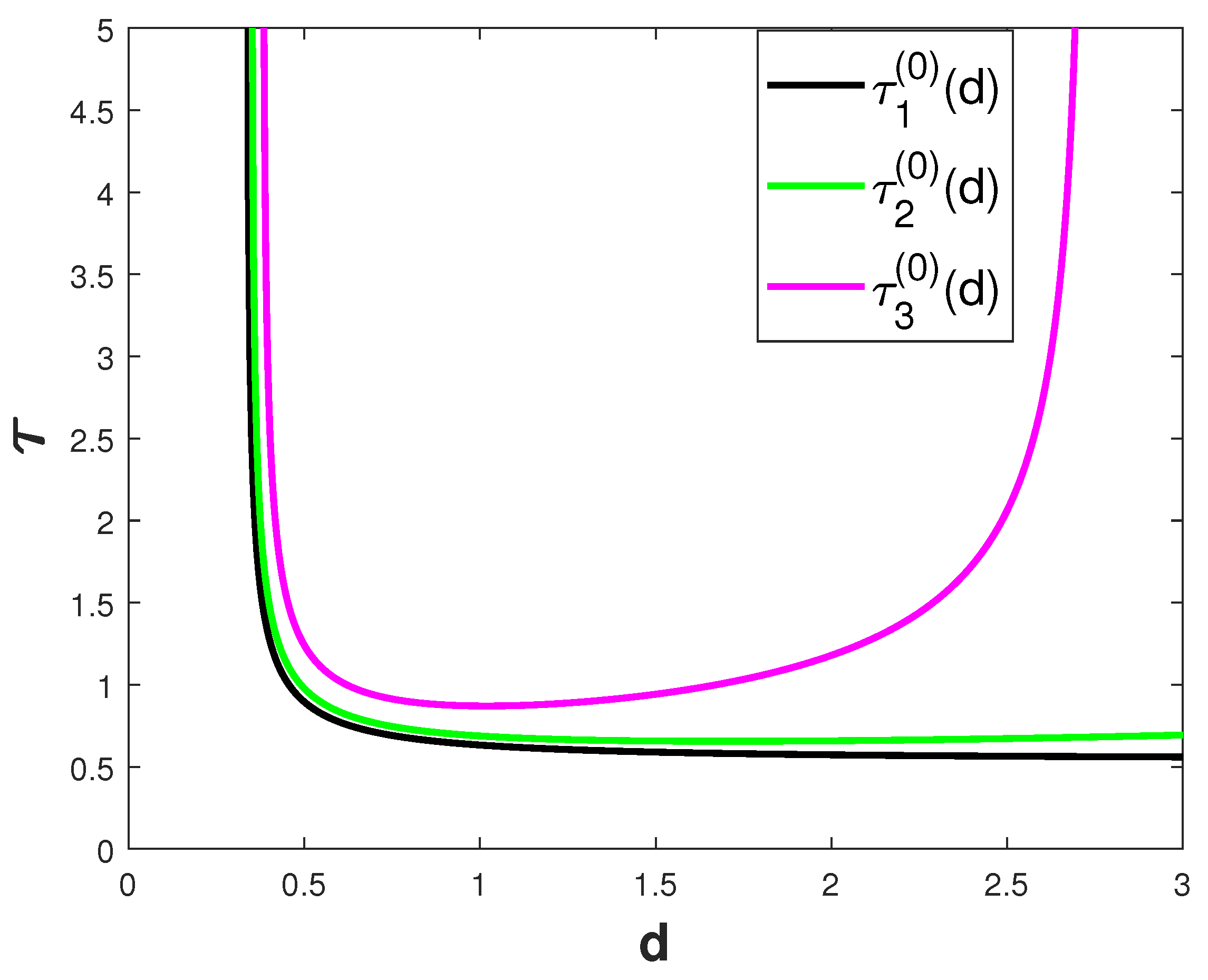
Figure 2.
is stable for , where . The initial value is , the parameters are given in (P1).
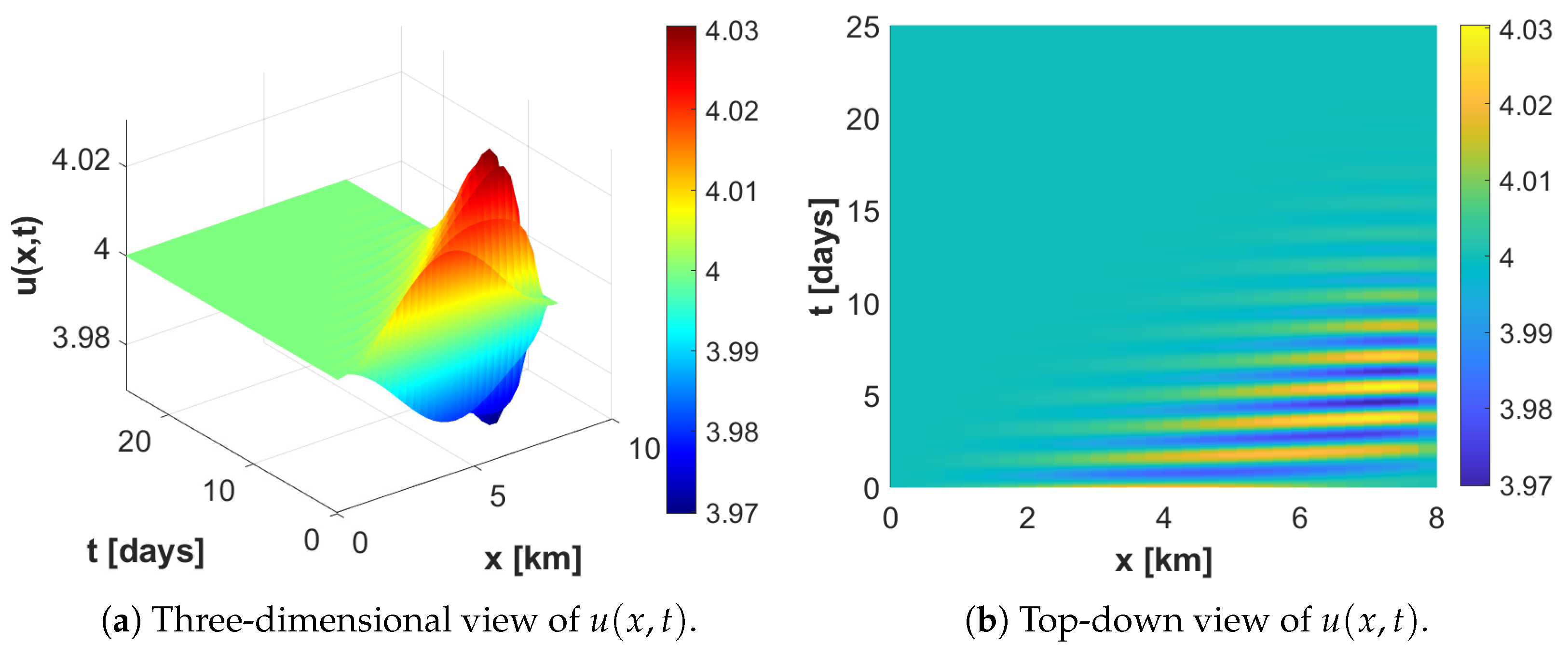
Figure 3.
A periodic soluton bifurcated from the positive steady state is stable for . The initial value is , the parameters are given in (P1).
Figure 3.
A periodic soluton bifurcated from the positive steady state is stable for . The initial value is , the parameters are given in (P1).
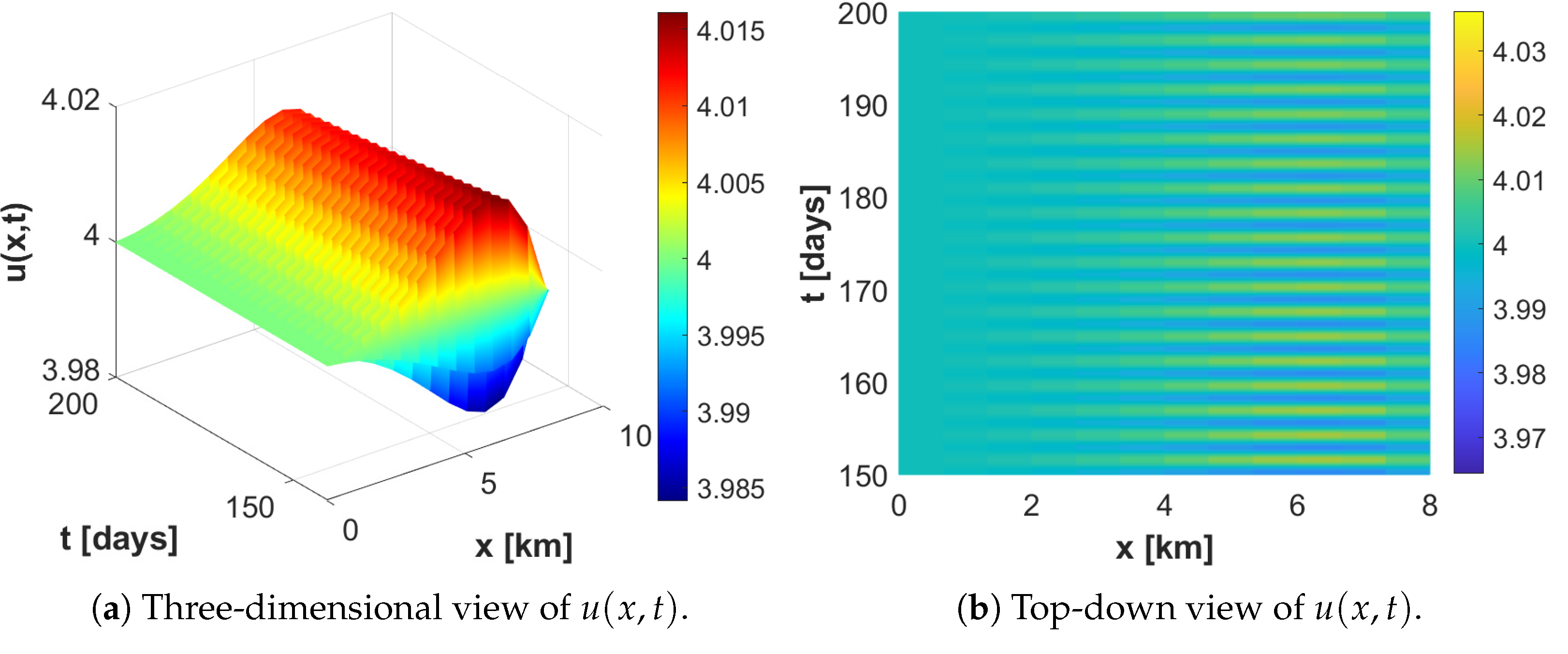
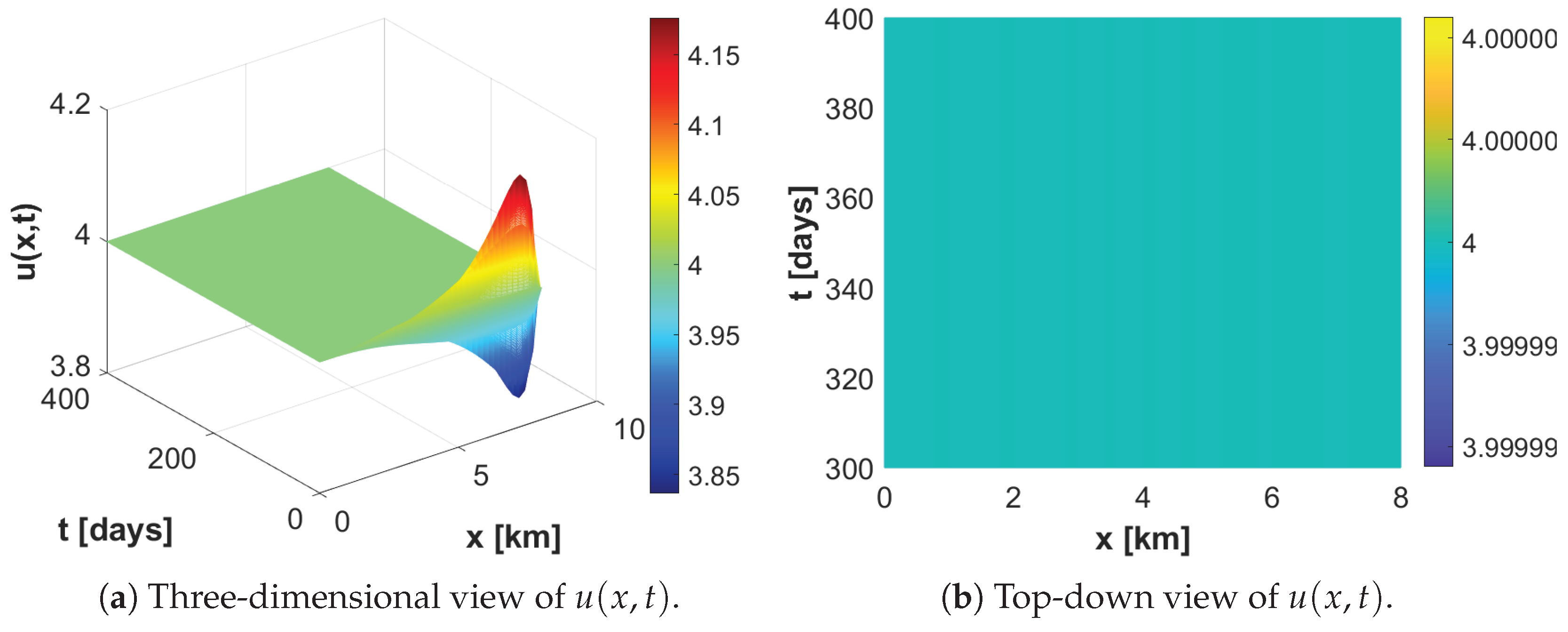
Figure 4.
The positive steady state is stable for . The initial value is , the parameters are given in (P2).
Figure 4.
The positive steady state is stable for . The initial value is , the parameters are given in (P2).
Disclaimer/Publisher’s Note: The statements, opinions and data contained in all publications are solely those of the individual author(s) and contributor(s) and not of MDPI and/or the editor(s). MDPI and/or the editor(s) disclaim responsibility for any injury to people or property resulting from any ideas, methods, instructions or products referred to in the content. |
© 2025 by the authors. Licensee MDPI, Basel, Switzerland. This article is an open access article distributed under the terms and conditions of the Creative Commons Attribution (CC BY) license (http://creativecommons.org/licenses/by/4.0/).
Copyright: This open access article is published under a Creative Commons CC BY 4.0 license, which permit the free download, distribution, and reuse, provided that the author and preprint are cited in any reuse.


