
Submitted:
11 August 2023
Posted:
14 August 2023
You are already at the latest version
Abstract
This study proposes a nonlinear mathematical model of virus transmission based on the SEIR model. In this study, the interaction between viruses and immune cells is investigated using phase-space analysis of a mathematical model. Specifically, it is focused on the dynamics and stability behavior of the mathematical model of a virus spread in a population and its interaction with human immune systems cells. The endemic equilibrium points are found and local stability analysis of all equilibria points of the related model is obtained. Further, the global stability analysis either, at disease-free equilibria, or in endemic equilibria is discussed by constructing the Lyapunov function which shows the validity of the concern model exists. Finally, a simulated solution is achieved and the relationship between viruses and immune cells is highlighted.
Keywords:
Mathematical modeling
; Virus
; Immune system
; Stability of dynamical systems
; SEIR
1. Introduction
Mathematical modeling of biological processes is a field of research that facilitates our understanding of complex biological systems and variables by simulating and analyzing several biological scenarios through specific models based on mathematical theories [1,2,3]. It provides a robust approach to describe mechanisms behind the dynamics occurring in biological processes by melting mathematical theories and models in the same pot with biological simulations [1]. This approach is playing a crucial role in predicting the spread rates of various major public health problems caused by viral diseases such as Ebola [4], Influenza [5], Cancer [6], Zika [7], Usutu [8], and Covid-19 [9].
Simultaneously, the field of mathematical modeling and simulations has gained considerable attention in various areas of human physiology, e.g., the analysis of muscle structure [10] and the study of brain activity [11,12]. Furthermore, mathematical modeling is also actively used to optimize medication usage and treatment process [13,14,15]. In this study, we focused mainly on modeling and simulating the spread of viruses and the behavior of cells in the human immune system through the dynamical modeling approach. Dynamic models are widely recognized for their pivotal role in describing the interactions among uninfected cells, free viruses, and immune responses [16,17,18,19]. The latest study findings highlighted the ability of complex models to describe human biology. For instance, Nowak et al. proposed a three-dimensional dynamic model for viral infection, which utilized numerical methods from autonomous dynamical systems [17,18,19]. Giesl and Wendland characterized a Lyapunov function as a solution of a suitable linear first-order partial differential equation approximating it using radial basis functions [20]. Yang and Wang formulated a mathematical model employing non-constant transmission rates, which varied with environmental conditions and the epidemiological status and reflected the impact of the ongoing disease control measures [21]. Despite significant efforts in designing mathematical models for virus dynamics, characterizing their behavior remains challenging. Even though several models have been proposed over the past two decades, their results bring different outcomes. However, a deterministic compartmental (SEIR) model has been successfully devised [22]. In mathematical epidemiology, numerous models have been proposed to analyze and predict epidemic outbreaks [23,24,25]. One such approach is the stereographic Brownian diffusion epidemiology model (SBDiEM), which provides a novel spatial perspective for the dynamic publishing, prediction, and modeling of infectious diseases [26,27]. The SBDiEM model can be adapted to identify past outbreaks and track the spread of viruses, offering valuable insights for national health systems, international stakeholders, and policymakers, thereby contributing to innovative perspectives in the field [28].
Kahajji et al. conducted a study focusing on the transmission dynamics of viruses, developing a separate mathematical model to describe the spread of the virus among animals in different regions. Their study highlights the importance of implementing effective campaigns to prevent individuals from moving between regions, promoting participation in quarantine centers, utilizing awareness campaigns targeted at virus prevention, and implementing security measures and health protocols within the region [29]. They estimated outbreak dynamics through mathematical modeling and provided decision guidelines for successful outbreak control. Furthermore, their model provided a valuable tool for estimating vaccination effectiveness and quantifying the impact of relaxing political measures, such as total lockdowns, shelter-in-place orders, and travel restrictions, for both low-risk subgroups and the population as a whole [30]. Numerous studies have highlighted the importance of models and simulations in understanding complex biological phenomena and tackling emerging diseases. However, the diversity of biological factors affecting human health and the emergence of new diseases warrants further exploration.
Moreover, the mathematical approaches identified by the World Health Organization (WHO) can be essential in providing evidence-based information to healthcare decision-makers and policymakers [31].
In this study, we have theorized a nonlinear mathematical model of virus transmission based on the SEIR model. We consider the following mathematical model concerning the initial value problem for the following nonlinear systems:
where , , and denotes the concentration of uninfected cells, infected cells, effector immune cells, and free viruses at time , respectively.
Uninfected cells are supplied at a rate a, and uninfected hepatocytes (target cells, T) are infected by virus V at . They are () that die naturally at the rate q is the rate constant characterizing infection of the infected cells. Effector cells mediate infection by eliminating productively infected cells at a rate of . Effector immune cells E are supplied to the presence of tumor cells, stimulating the immune response. The virus activates the effector immune cells at the rate of . The infected cells produce new viruses at the rate of b during their life. The constant is the rate at which the viruses are cleared [32,33,34]. They worked on the local and global dynamic model of cancer tumor growth [35]. Recently, studies have been carried out on dynamic models [6,35,36,37].
2. Boundedness and Dissipativity
In this section, we showed that the model is bounded by negative divergence, positively invariant with respect to a region in and dissipative. As we are interested in biologically relevant solutions of the system, the next results show that the positive octant is invariant and that the upper limits of trajectories depend on the parameters.
We put
Then the problem is reduced the following form:
Let
Here,
Consider the problem with
Condition 1.
Assume the following assumption is satisfied
Theorem 1.
Let the Condition 1 holds. Then the system is with the negative divergence and is dissipative in the domain .
Proof.
Indeed, from and we have
Hence, by Condition 1, the system is dissipative on the domain but there is no definition of Condition 1. □
3. The Local Stability of Equilibria Points
In this section, we derive the stability properties of equilibria points of the system . Let
Condition 2.
Let
Theorem 2.
Assume that the Condition 2 is satisfied. There is a point that is a equilibria points of the system in .
Proof.
It is sufficient to find the solution of the following system of algebraic equation in , , , :
From first and second equations we have
From third and fourth equations we get
If we get that . By , then we dedused that . Hence, from we have
Thus we obtain that the system have a unique equalibria point , where
□
Remark 1.
For the point to have the biological meaning of stability point , it should be:
We show here, the following results:
Theorem 3.
Assume that the Condition 2 is satisfied. Suppose the estimate holds. Then the point is locally stable point for the system of
Proof.
Consider the linearized matrix of , i.e. the Jacobian matrıx according to system at point is the following:
where
□
The eigenvalues of the matrix A can found as the solutions of the following equations
Let we put
i.e. , and are the eigenvalues of A. Then other solutions of A can be obtained by solving the equation
By solving the equation we get the fourth eigenvalue of the matrix A
For local stability of the system it is sufficient to show that all eigenvalues of the matrix A are negative. Indeed, by and , we have
By assumption , and by we see that,
Hence by we get
Moreover, it should be
The estimate satisfies if:
or
Since the second inequality in satisfied for all , when
i.e. by if
By assumption , the above inequality is satisfied when
that it is clear that holds for all . Since for all , the inequality is not satisfied in . Hence we obtained that all eigenvalues of the matrix are negative under our assumptions.
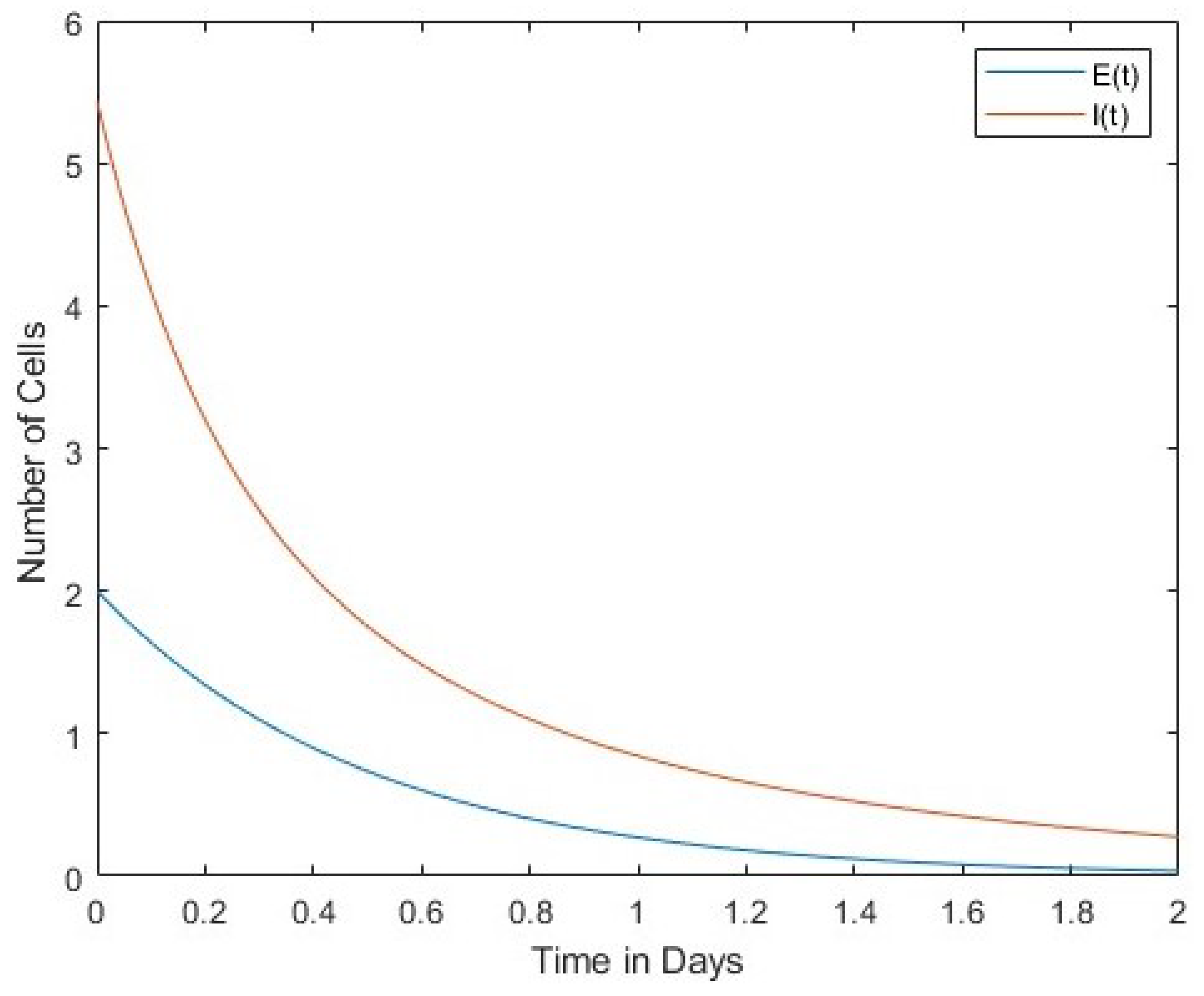
In Figure 1 we compare the number of viruses with the number of infected cells. Both the number of viruses and the number of infected cells decrease over time. The second Figure 2 compares the number of viruses with the number of uninfected cells. In this case, the rates of change between the two are in inverse proportion to each other. Finally, Figure 3 shows a comparison between the number of infected cells and the number of effector immune cells. It is noticeable that both the infected cells and the immune cells in this figure rapidly decrease over time.
4. Lyapunov Stability of Equilibria Points
Let is a equilibria point, where is defined by . In this section, we show the following results: Let be the linearized matrix with respect to equilibria point defined by , i.e.
where are defined by . We consider the Lyapunov equation
It is clear that
reduced to the following equation
where
Main and associated determinants of the system in is the following
...
We assume that . Then by by solving with respect to by Kramer method, we obtain
Theorem 4.
Assume the Condition 2 holds, . Suppose such that , , for , when . Then the system is asymptotically stable at the equilibria point in the sense of Lyapunov.
Proof.
By assumptions the function associated with tha matrix A defined by
is positive defined in Hence, all eigenvalues of the the matrix is positive in , i.e. is a positive defined Lyapunov function candidate (see e.g. ). By . We need now to determine a domain on which is negatively defined. By assuming , we will find the solution set of the following inequality
Hence, the system is asymptotically stabile at in the Lyapunov sense when,
i.e. the system is asymptotically stabile at in the Lyapunov sense in the following domain
□
Theorem 5.
Assume the Condition 2 holds, . Suppose such that , and for when . Then the system is asymptotically stable at the equilibria point in the sense of Lyapunov.
Proof.
when
Then by reasoning as in Theorem 4. we obtain the conclusion. □
Remark 2.
Assume the Condition 2 holds, . Suppose such that , , for and for when or for and for when .
Similar way as in Theorem 4 we get that Then the system is asymptotically stable at the equilibria point in the sense of Lyapunov.
5. Discussion
The spread rate of the virus in the population and its interaction with immune system cells were examined through a SEIR model. Stability analysis was performed by finding the equilibrium points of the nonlinear model created with four variables. Specifically, these variables and were the concentration of uninfected cells, infected cells, effector immune cells, and free viruses, respectively. An approximate solution has been pursued since theoretical nonlinear equations usually have no deterministic solution. Here, the coefficient of the variables is considered equal to In addition, global stability analysis was discussed by constructing the Lyapunov function, which validates the robustness of the dynamic model in disease-free equilibrium or endemic equilibrium. This analysis provides an understanding of the long-term behavior of the model and its impact on the progression of viral infections.
In Figure 1 and Figure 2, the interaction of the virus between infected cells and normal uninfected cells was studied. Figure 1 shows a direct proportionality between cells’ dynamics, while Figure 2 shows an inversion of the cells’ dynamics. Finally, Figure 3 shows the interaction between immune and infected cells. This Figure shows a direct proportionality between immune and infected cell dynamics.
The nonlinear model aimed to capture the interaction among the virus cells in different conditions, i.e., when virus cells are in contact with infected cells, when the virus is in relation with uninfected cells, or when there are infected and uninfected cells alone. It is worth noting that these relationships were obtained within certain mathematical conditions, which can affect the model results. The real-life condition could be more complex than those represented in this study. However, this model could pose a remarkably well-structured nonlinear mathematical fashion for analyzing how virus cells interact with the other cells within a human body. Moreover, it provides interesting information on the process dynamics over time, i.e., from the past to the future.
Future studies need to focus and validate the results of the model through experimental studies and physical observations. Although the model provides important views of the interaction dynamics between virus cells and other cells in the human body, real-life conditions may be more complex than those represented in this study. Therefore, empirical studies would be crucial to validate the accuracy and applicability of the model in a more real-life scenario.
6. Conclusion
In this work, the interaction between viruses and immune cells was investigated. Cases of normal cells infected with the virus were also included in the model. A four-variable dynamic model of normal cells, infected cells, effector immune cells, and free viruses was constructed. Equilibrium points of this mathematical model were found, and Lyapunov stability analyses were performed. Relationships among the virus, the infected and uninfected cells were discussed, as reported in Figure 1, Figure 2 and Figure 3.
A directly proportional relationship between viruses and infected cells was found in the decrease and increase of the cells’ dynamics, as shown in Figure 3. In Figure 2, virus and uninfected cells were compared. Rates of change are inversely proportional to each other. Infected and immune cells are proportionally reduced rapidly in Figure 3.
This model, which could be validated by clinical trials, poses itself as a possible aid for decision-makers to structure their health policies according to evidence-based mathematical models.
References
- Chou, C.S.; Friedman, A. Introduction to mathematical biology; Springer, 2016.
- Britton, N.F.; Britton, N. Essential mathematical biology; Vol. 453, Springer, 2003.
- Jones, D.S.; Plank, M.; Sleeman, B.D. Differential equations and mathematical biology; CRC press, 2009.
- Rachah, A.; others. Analysis, simulation and optimal control of a SEIR model for Ebola virus with demographic effects. Communications Faculty of Sciences University of Ankara Series A1 Mathematics and Statistics 2018, 67, 179–197.
- Etbaigha, F.; R. Willms, A.; Poljak, Z. An SEIR model of influenza A virus infection and reinfection within a farrow-to-finish swine farm. PLOS one 2018, 13, e0202493.
- Shakhmurov, V.B.; Kurulay, M.; Sahmurova, A.; Gursesli, M.C.; Lanata, A. Interaction of Virus in Cancer Patients: A Theoretical Dynamic Model. Bioengineering 2023, 10, 224. [CrossRef]
- Dantas, E.; Tosin, M.; Cunha Jr, A. Calibration of a SEIR–SEI epidemic model to describe the Zika virus outbreak in Brazil. Applied Mathematics and Computation 2018, 338, 249–259.
- Cheng, Y.; Tjaden, N.B.; Jaeschke, A.; Lühken, R.; Ziegler, U.; Thomas, S.M.; Beierkuhnlein, C. Evaluating the risk for Usutu virus circulation in Europe: comparison of environmental niche models and epidemiological models. International journal of health geographics 2018, 17, 1–14. [CrossRef]
- Iwata, K.; Miyakoshi, C. A simulation on potential secondary spread of novel coronavirus in an exported country using a stochastic epidemic SEIR model. Journal of clinical medicine 2020, 9, 944. [CrossRef]
- Battista, N.A.; Baird, A.J.; Miller, L.A. A mathematical model and MATLAB code for muscle–fluid–structure simulations. Integrative and comparative biology 2015, 55, 901–911.
- Vatov, L.; Kizner, Z.; Ruppin, E.; Meilin, S.; Manor, T.; Mayevsky, A. Modeling brain energy metabolism and function: a multiparametric monitoring approach. Bulletin of mathematical biology 2006, 68, 275–291. [CrossRef]
- Bakshi, S.; Chelliah, V.; Chen, C.; van der Graaf, P.H. Mathematical biology models of Parkinson’s disease. CPT: pharmacometrics & systems pharmacology 2019, 8, 77–86. [CrossRef]
- Durrant, J.D.; McCammon, J.A. Molecular dynamics simulations and drug discovery. BMC biology 2011, 9, 1–9. [CrossRef]
- Lavé, T.; Parrott, N.; Grimm, H.; Fleury, A.; Reddy, M. Challenges and opportunities with modelling and simulation in drug discovery and drug development. Xenobiotica 2007, 37, 1295–1310. [CrossRef]
- Salo-Ahen, O.M.; Alanko, I.; Bhadane, R.; Bonvin, A.M.; Honorato, R.V.; Hossain, S.; Juffer, A.H.; Kabedev, A.; Lahtela-Kakkonen, M.; Larsen, A.S.; others. Molecular dynamics simulations in drug discovery and pharmaceutical development. Processes 2020, 9, 71. [CrossRef]
- Anderson, R.M.; May, R.M. Infectious diseases of humans: dynamics and control; Oxford university press, 1991.
- Nowak, M.; May, R.M. Virus dynamics: mathematical principles of immunology and virology: mathematical principles of immunology and virology; Oxford University Press, UK, 2000.
- Nowak, M.A.; Bangham, C.R. Population dynamics of immune responses to persistent viruses. Science 1996, 272, 74–79.
- Perelson, A.S.; Nelson, P.W. Mathematical analysis of HIV-1 dynamics in vivo. SIAM review 1999, 41, 3–44. [CrossRef]
- Giesl, P.; Wendland, H. Numerical determination of the basin of attraction for exponentially asymptotically autonomous dynamical systems. Nonlinear Analysis: Theory, Methods & Applications 2011, 74, 3191–3203. [CrossRef]
- Yang, C.; Wang, J. A mathematical model for the novel coronavirus epidemic in Wuhan, China. Mathematical biosciences and engineering: MBE 2020, 17, 2708. [CrossRef]
- Tang, B.; Wang, X.; Li, Q.; Bragazzi, N.L.; Tang, S.; Xiao, Y.; Wu, J. Estimation of the transmission risk of 2019-nCov and its implication for public health interventions (January 24, 2020). Available at SSRN 3525558 2020.
- Kao, R.R. The role of mathematical modelling in the control of the 2001 FMD epidemic in the UK. TRENDS in Microbiology 2002, 10, 279–286.
- Chowell, G.; Sattenspiel, L.; Bansal, S.; Viboud, C. Mathematical models to characterize early epidemic growth: A review. Physics of life reviews 2016, 18, 66–97. [CrossRef]
- Hyman, J.M.; Stanley, E.A. Using mathematical models to understand the AIDS epidemic. Mathematical Biosciences 1988, 90, 415–473. [CrossRef]
- Logeswari, K.; Ravichandran, C.; Nisar, K.S. Mathematical model for spreading of COVID-19 virus with the Mittag–Leffler kernel. Numerical Methods for Partial Differential Equations 2020.
- Wang, Y.; Xu, C.; Yao, S.; Wang, L.; Zhao, Y.; Ren, J.; Li, Y. Estimating the COVID-19 prevalence and mortality using a novel data-driven hybrid model based on ensemble empirical mode decomposition. Scientific Reports 2021, 11, 21413. [CrossRef]
- Bekiros, S.; Kouloumpou, D. SBDiEM: a new mathematical model of infectious disease dynamics. Chaos, Solitons & Fractals 2020, 136, 109828. [CrossRef]
- Khajji, B.; Kada, D.; Balatif, O.; Rachik, M. A multi-region discrete time mathematical modeling of the dynamics of Covid-19 virus propagation using optimal control. Journal of Applied Mathematics and Computing 2020, 64, 255–281. [CrossRef]
- Peirlinck, M.; Linka, K.; Sahli Costabal, F.; Kuhl, E. Outbreak dynamics of COVID-19 in China and the United States. Biomechanics and modeling in mechanobiology 2020, 19, 2179–2193. [CrossRef]
- Houben, R.M.; Dodd, P.J. The global burden of latent tuberculosis infection: a re-estimation using mathematical modelling. PLoS medicine 2016, 13, e1002152.
- Alofi, B.; Azoz, S. Stability of general pathogen dynamic models with two types of infectious transmission with immune impairment. AIMS Mathematics 2021, 6, 114–140. [CrossRef]
- Wang, S.; Zou, D. Global stability of in-host viral models with humoral immunity and intracellular delays. Applied Mathematical Modelling 2012, 36, 1313–1322. [CrossRef]
- Siettos, C.I.; Russo, L. Mathematical modeling of infectious disease dynamics. Virulence 2013, 4, 295–306. [CrossRef]
- Shakhmurov, V.; Sahmurova, A. The local and global dynamics model of a cancer tumor growth. Applicable Analysis 2021, pp. 1–25. [CrossRef]
- Shakhmurov, V.; Maharramov, A.; Shahmurzada, B. The local and global dynamics of a cancer tumor growth and chemotherapy treatment model. arXiv preprint arXiv:1803.05330 2018.
- Ojo, M.M.; Peter, O.J.; Goufo, E.F.D.; Panigoro, H.S.; Oguntolu, F.A. Mathematical model for control of tuberculosis epidemiology. Journal of Applied Mathematics and Computing 2023, 69, 69–87.
Figure 1.
We compare infected cells (I(t)) and free viruses (V(t)). They are and .
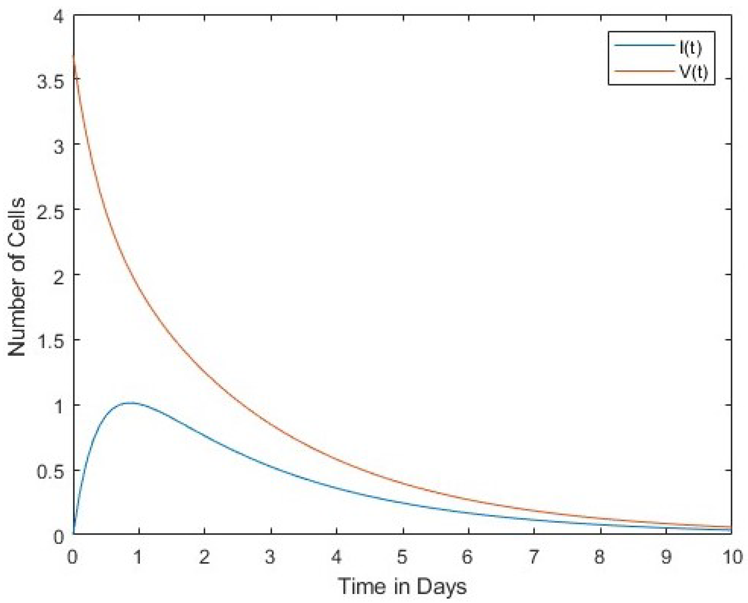
Figure 2.
We compare uninfected cells (T(t)) and free viruses (V(t)). They are and .
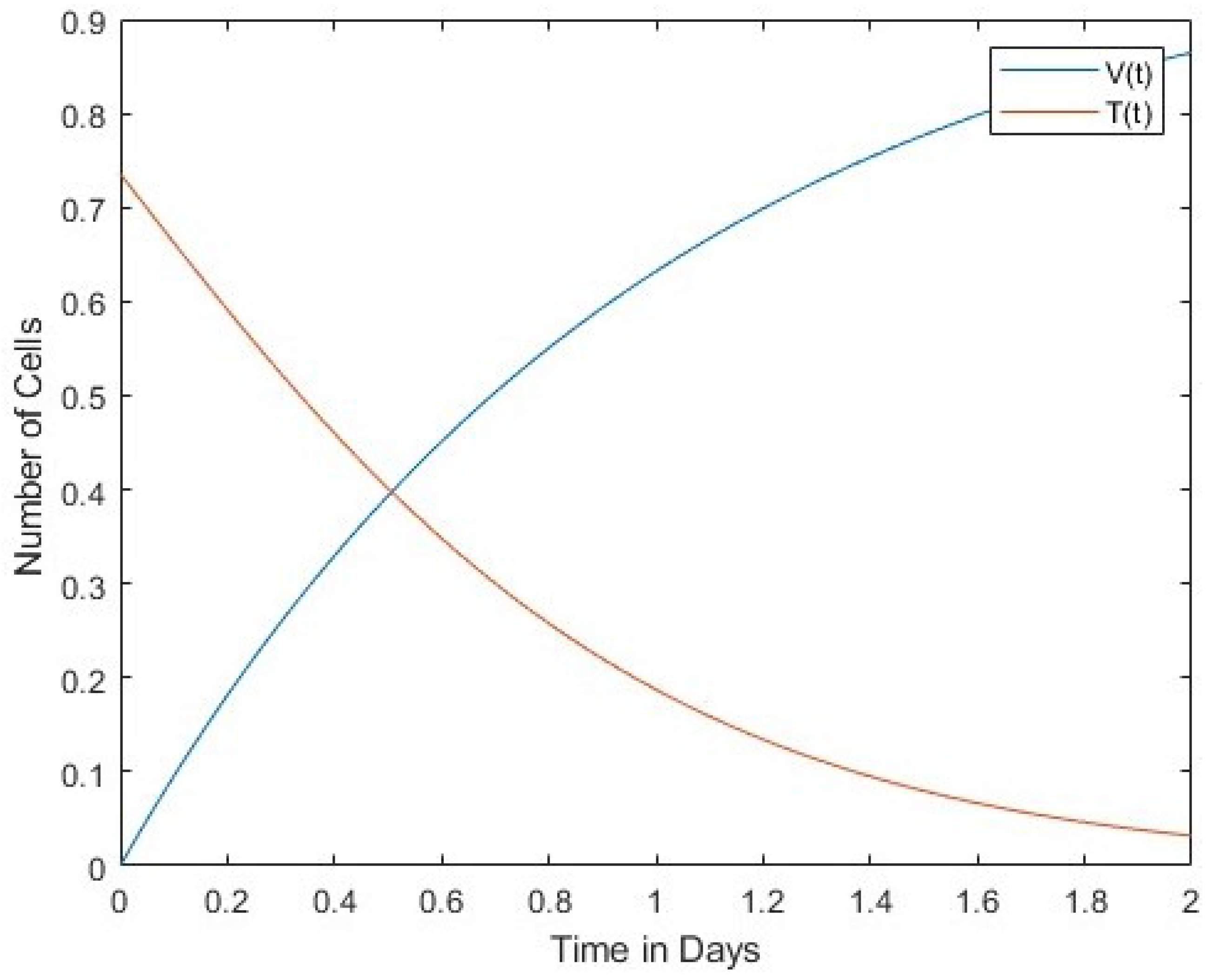
Figure 3.
We compare effector immune cells (E(t)) and infected cells (I(t)). They are and .
Disclaimer/Publisher’s Note: The statements, opinions and data contained in all publications are solely those of the individual author(s) and contributor(s) and not of MDPI and/or the editor(s). MDPI and/or the editor(s) disclaim responsibility for any injury to people or property resulting from any ideas, methods, instructions or products referred to in the content. |
© 2023 by the authors. Licensee MDPI, Basel, Switzerland. This article is an open access article distributed under the terms and conditions of the Creative Commons Attribution (CC BY) license (http://creativecommons.org/licenses/by/4.0/).
Copyright: This open access article is published under a Creative Commons CC BY 4.0 license, which permit the free download, distribution, and reuse, provided that the author and preprint are cited in any reuse.


