Submitted:
02 December 2025
Posted:
04 December 2025
You are already at the latest version
Abstract
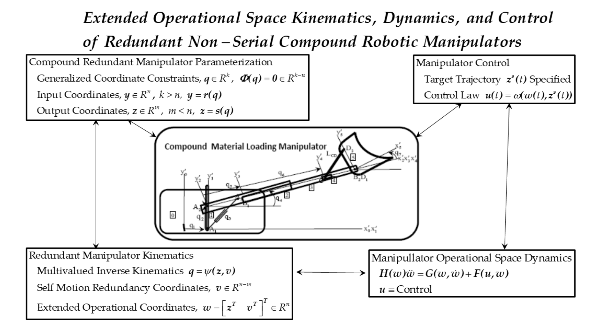
An extended operational space kinematics and dynamics formulation is presented for control of redundant non-serial compound robotic manipulators. A broad spectrum of high load capacity non-serial manipulators used in earth moving, material handling, and construction applications is addressed. Departing from conventional approaches that rely on Jacobian pseudoinverses and local null-space projections, a globally valid, differential geometry-based, multi-valued inverse kinematic mapping is defined at the configuration level, with explicit self-motion parameterization of manipulator redundancy. The formulation yields coupled second-order ordinary differential equations of manipulator dynamics on the product space of task variables and self-motion coordinates. This enables direct integration of system dynamics with control strategies, such as model predictive control or feedback design, while maintaining task constraint compliance. The methods presented are validated through simulation and control of a multi-degree of redundancy non-serial compound material loader manipulator, demonstrating advantages in generality, numerical accuracy, and trajectory smoothness.
Keywords:
redundant non-serial robots
; robot dynamics
; extended operational space robot control
1. Introduction
Redundant robotic manipulators offer flexibility for achieving tasks such as obstacle avoidance, joint limit avoidance, and posture optimization. However, classical modelling and control strategies have been limited to serial manipulators and rely on velocity-level inverse kinematics using Jacobian pseudoinverses and null-space projection techniques [3,4,23,24]. These approaches are inherently local and can suffer from numerical drift, instability near singularities, and difficulties in maintaining secondary objectives over extended trajectories. Recent papers by the authors employs differential geometry and modern methods of multibody dynamics that avoid use of Lagrange multipliers and resolve these deficiencies for redundant robotic manipulators [17,18,20]. This paper extends these results to a dynamically consistent approach that is globally valid on singularity free components of non-serial compound manipulator configuration space. Building on a configuration-level inverse kinematic mapping that presents all inverse kinematic solutions as functions of operational space parameters, coupled second-order ordinary differential equations (ODE) of dynamics are constructed in the product space of task variables and self-motion coordinates. This framework eliminates the need for projection-based redundancy resolution and provides a control-ready ODE formulation that is applicable for a broad spectrum of non-serial compound manipulator architectures.
Goals of the paper are twofold: (i) present a new dynamics and control formulation in an accessible style for researchers and control engineers, and (ii) benchmark its performance using a multi-degree of redundancy example. This work aims to bridge a significant gap between geometric modeling of redundant non-serial compound manipulators and their application in planning and control.
2. Background on Redundant Non-Serial Compound Manipulator Modeling and Control
2.1. Methods Adapted from Redundant Serial Manipulators
In redundant serial manipulators, an explicit input-output forward kinematic relation exists, in the form [4,20]
where input and output coordinates are denoted , with . Here, is k-dimensional Euclidean space with elements in the form of column vectors . Bold symbols are vectors and matrices.
The inverse kinematics problem associated with Eq. (2.1) has infinitely many solutions. Classical approaches resolve this redundancy by operating at the velocity level [3,33] ,
where is the Moore-Penrose pseudoinverse [4,32] of , and is arbitrary. Although effective in some non-serial settings, such methods are differential in nature and require integration to recover configurations. They can exhibit numerical instability and are often sensitive to singularities. This velocity space generalized inverse approach has been adapted for use in parallel redundant manipulators, but without notable success [14,15].
Task-priority methods and control in operational space originated in the serial manipulator setting; e.g., [23,30], provide hierarchical frameworks for multiple objectives, but rely on local Jacobian-based approximations and projections that lead to serious problems, especially in non-serial compound manipulators.
The concept of self-motion of serial manipulators introduced in [3] has been adapted in the present research for use with non-serial compound manipulator applications.
2.2. Constrained Operational Space Dynamics
In a formulation introduced in [8], the multiplier form of the constrained equation of motion is mapped into task space using the dynamically consistent inverse of a Jacobian that characterizes both task and constraint spaces. The resulting task space equation of motion is then partitioned into an equation corresponding to the motion, and an equation corresponding to constraint forces. One begins by expressing the multiplier form of the constrained equation of motion. The d’Alembert variational equation of motion for the manipulator with holonomic constraints is
for all ; i.e., for all such that [10,13,21,28]. This implies
subject to holonomic constraints,
where is a vector of Lagrange multipliers that determine constraint forces. The task velocity relationship is
and the constraint velocity condition is
Concatenating these relationships into a single matrix relation,
where the notation represents a quantity that is formed from the composition of task and constraint terms. The applied generalized force can be decomposed into a task/constraint space component and a null space component, as in [8],
where is the component of applied task space force acting along the constraint direction. Equation (2.8) can thus be written as
Mapping Eq. (2.9) into task space by premultiplying by ,
This yields
and
where the constraint condition, , has been imposed. This yields the following identities:
While Eq. (2.12) expresses system task-constraint dynamics, it is useful to partition it in the following manner:
This partitioning yields an equation corresponding to task space control force,
and an equation corresponding to constraint forces,
The constraint force vector will always arise so as to satisfy Eq. (2.15), as dictated by constraint consistency. The component of applied task space force, , acting along the constraint direction has no impact on motion of the task. Its only effect is on constraint forces (values of λ) that arise. Thus, all choices for result in equivalent motion of the system.
The dynamics are derived from Eqs. (2.15) and (2.16), as demonstrated in [9],
The term is the constraint null space matrix, is the task/constraint space mass matrix, is the task/constraint space centrifugal and Coriolis force vector, is the task/constraint space gravity vector, and is the task/constraint null space projection matrix. These terms are given in [8,9] as
The term is the constraint space mass matrix, which reflects system inertia projected onto the constraint, is the vector of centrifugal and Coriolis forces projected onto the constraint, and is the vector of gravity forces projected onto the constraint,
2.3. Redundant Parallel Manipulators
Redundant manipulators comprised of a single moving platform as output with six spatial degrees of freedom, whose position and orientation are controlled by parallel legs with more than six input coordinates have received significant attention in the engineering literature [14,15,26]. Inverse kinematics approaches in these applications have, however, been ad hoc or adaptations of problematic generalized inverse velocity approaches adapted from the serial manipulator literature. A contribution to the redundant parallel manipulator literature [5] established the reality that excess generalized coordinates are required to treat this class of redundant manipulator. This reality is addressed in redundant non-serial compound manipulators addressed herein.
3. A Redundant Non-Serial Compound Material Loader Manipulator
In contrast with the foregoing, the approach presented in this paper constructs an explicit inverse kinematic mapping at the position/configuration level. A unified approach is employed for redundant non-serial compound manipulators, allowing the full set of inverse kinematic solutions to be represented analytically [18]. This enables direct formulation of dynamics in a form that is suitable for implementation of control laws in the space of task and self-motion redundancy coordinates, without projection into a Jacobian null space. The unified approach presented herein for non-serial redundant manipulators is an extension of prior developments that used idealized small-scale manipulators to illustrate the formulation [18]. A multi-degree of redundancy example is used herein to motivate the approach presented, in a rigorous but tutorial style, with numerical results that verify accuracy and practicality of the approach.
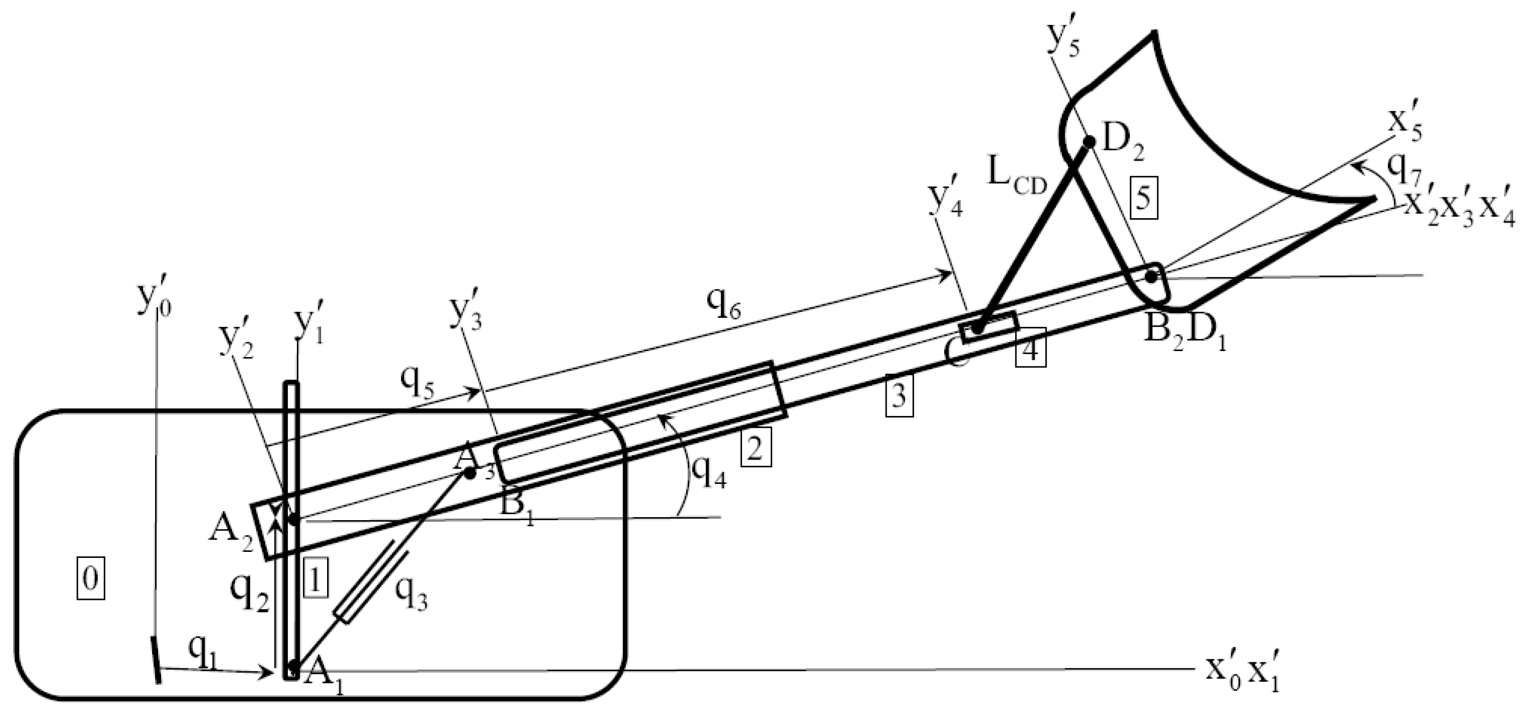
Kinematics of a five-body planar material loading compound manipulator [18] of Figure 3.1 are defined by unit length horizontal and vertical vectors , and the following vectors that locate key points on the manipulator in the global frame as functions of generalized coordinates :
where is the distance between points A and B, is the length of body 3, and .
Figure 3.1.
Compound Material Loader Loops comprised of (1) bodies 0, 1, 2, and slider that define the length of actuator , which is not contained in a joint (2) bodies 3, 4, and 5 that define the fixed length of bar are written in algebraic form as.
Figure 3.1.
Compound Material Loader Loops comprised of (1) bodies 0, 1, 2, and slider that define the length of actuator , which is not contained in a joint (2) bodies 3, 4, and 5 that define the fixed length of bar are written in algebraic form as.
4. Redundant Compound Manipulator Kinematics, Dynamics, and Control
4.1. Basics of Compound Redundant Manipulator Kinematics
Many important redundant compound manipulators, or simply compound manipulators, contain kinematic and/or actuator closed loops and are not characterized by kinematic models of redundant serial manipulators. Their kinematics are defined by input coordinates , output coordinates , , and generalized coordinates , . Generalized coordinates satisfy twice continuously differentiable constraints,
and determine input and output coordinates as
where are twice continuously differentiable functions.
Redundant compound manipulators are encountered in applications involving heavy loads and high precision requirements. They also arise when Euler parameters with excess variables are employed that are subject to a normalization constraint to define orientation in space [21].
There is little literature on redundant compound manipulators. Conconi and Carricato [5] studied redundant manipulators using screw coordinates and showed that manipulators containing closed kinematic loops require inclusion of generalized coordinates and holonomic constraints in the kinematic model. De Sapio, Khatib, Jain, and coworkers addressed redundant compound manipulators using an operational space methodology based on a velocity formulation and Lagrange multipliers [9,22,23]. While some positive results have been obtained, well known problems associated with the velocity approach [7,19,31] remain unresolved in compound manipulator kinematics and dynamics.
4.1.1. Manipulator Configuration Space
4.1.2. Assembly Components
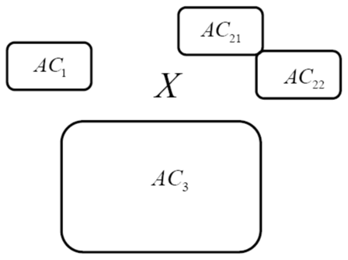
It is shown in [18] that if has full rank, X of Eq. (4.3) is a topological space that may be partitioned into maximal, disjoint, path connected assembly components that cover X, shown schematically in Figure 4.1. Configurations in disjoint closures of assembly components cannot be connected by a continuous path in X.
Figure 4.1.
Assembly Components of Manipulator Configuration Space.
4.1.3. Forward and Inverse Kinematics
Forward and inverse kinematics of compound manipulators are defined by composite equations comprised of Eqs. (4.1) and (4.2),
If for , the implicit function theorem [6] assures existence of a unique twice continuously differentiable solution
of Eq. (4.4) in a neighborhood of . Combining this with the second of Eqs. (4.2),
is a twice continuously differentiable forward kinematic mapping in a neighborhood of . While the mapping of Eq. (4.7) cannot generally be analytically defined, it can be evaluated accurately using Newton-Raphson iteration [1].
In contrast with the foregoing single-valued forward kinematic mapping, if for , the implicit function theorem assures existence of a twice continuously differentiable multi-valued solution
of Eq. (4.5), where is a vector of arbitrary coordinates, in a neighborhood of and . Combining this result with the first of Eqs. (4.2),
is a twice continuously differentiable multi-valued inverse kinematic mapping in a neighborhood of . This theoretical result can seldom be implemented analytically. It is implemented numerically in the following.
4.1.4. Singularity Free Assembly Components
It is shown in [18] that the regular compound manipulator configuration space
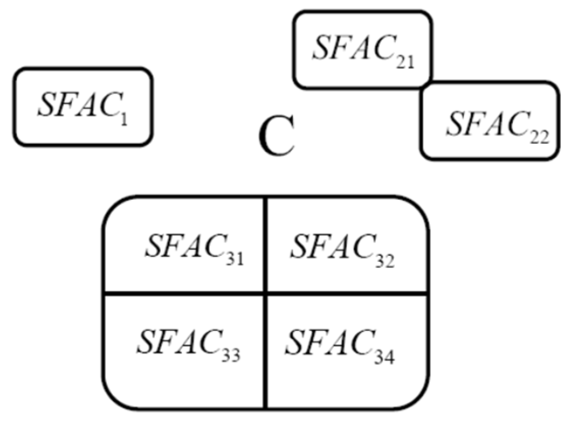
is a differentiable manifold that is partitioned into singularity free, path connected, assembly components that cover C, as shown schematically in Figure 4.2. Kinematics and dynamics may be carried out in each without encountering a singular configuration. It is impossible to connect configurations in different with singularity free continuous paths in C. These important results cannot be obtained if manipulator kinematics are defined in velocity space.
Figure 4.2.
Singularity Free Assembly Components.
4.1.5. Numerical Construction of a Multi-Valued Inverse Kinematic Mapping
To construct a multi-valued inverse kinematic mapping on a subset of with base point , define constant matrices and on such that
The matrix is computed using singular value decomposition [1,32]. Since the k linearly independent columns of span , every solution q of Eq. (4.5) in a neighborhood of may be represented as
where and . Note that and at .
The goal is to solve Eq. (4.5) with q of Eq. (4.12); i.e.,
for u as a function of z and v in a neighborhood of . The derivative of the left side of Eq. (4.13) with respect to u, evaluated at is , which is nonsingular. Thus, the implicit function theorem [6] implies existence of a unique, twice continuously differentiable solution
of Eq. (4.13) in a neighborhood of .
In a neighborhood of , in the space of operational coordinates , substituting u of Eq. (4.14) into Eq. (4.12),
Using the first of Eqs. (4.2),
is a twice continuously differentiable, multi-valued, inverse kinematic mapping in a neighborhood of . Multiplying Eq. (4.16) on the left by and using Eq. (4.7) yields a twice continuously, 1-to-1 relation between ,
Analysis in must be carried out on individual charts and transitioned to adjacent charts as manipulator configurations progress along a trajectory in , as shown schematically in Figure 4.3.
Figure 4.3.
Trajectory Along Charts in .
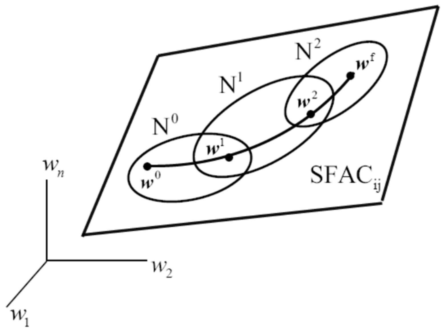
Note that if are periodic functions of time, so is ; i.e., this inverse kinematic mapping is locally cyclic, a property not enjoyed by inverse kinematics based on generalized matrix inverses [19,31].
With output fixed as z and arbitrary in a neighborhood of , Eq. (4.16) defines an infinite set of input coordinates,
This set is the manipulator self-motion manifold at z, for all v in a neighborhood of [29].
4.2. Compound Manipulator Dynamics
4.2.1. Input Space ODE of Dynamics
The d’Alembert variational equation of motion for the manipulator is
for all that are consistent with linearized forms of Eqs. (4.1) and (4.2) [21].
In , the solution of Eq. (4.4) satisfies . Differentiating with respect to y, so , which has full rank, since is nonsingular in and has full rank. Thus,
Differentiating this result with respect to t,
Since , with constant, differentiation with respect to t and manipulating yields [18]
where and .
Substituting of Eq. (4.22), of Eq.(4.6), Eq. (4.20), from Eq. (4.7), and into Eq. (4.19), . Since is arbitrary, the compound manipulator input space ODE of motion is
Since and is arbitrary, and the columns of span the null space of , is positive definite [21], hence nonsingular, so the ODE of Eq. (4.23) is well-posed [21].
4.2.2. Operational Space Velocity and Acceleration Kinematics
Differentiating Eq. (4.15) with respect to t,
Since is the solution of Eq. (4.13), . Differentiating this identity with respect to t,
From Eq. (4.11), is nonsingular. Since is continuous, is nonsingular in a neighborhood of and
is well defined and continuously differentiable in a neighborhood of .
Using Eq. (4.26) in Eq. (4.25),
In Eq. (4.24), this yields
In terms of differentials, this is
Suppressing arguments and manipulating the product on the left,
Thus, has full column rank, with left inverse
Differentiating Eq. (4.28) with respect to t,
where, from Eq. (4.28), . Writing Eq. (4.26) in the form , with constant, differentiating with respect to t, and manipulating [18],
Differentiating y of Eq. (4.16) with respect to t and using Eq. (4.27),
In terms of differentials, this is
4.2.3. Operational Space ODE of Dynamics
From Eq. (4.29), Eq. (4.34), and , , , and . Substituting these relations and Eq. (4.32) into Eq. (4.19), . Since is arbitrary, the compound manipulator operational space ODE of motion is
Since M is positive definite in the null space of [21] and for arbitrary , the linearly independent columns of the matrix H are in the null space of and is positive definite, hence nonsingular. Thus, the operational space ODE of Eq. (4.35) is well-posed [21].
For manipulator control, it may be helpful to write second order ODE in terms of z and v. Substituting of Eq. (4.31) and manipulating [18]
This operational space ODE of compound manipulator dynamics forms the foundation for a new approach to control of compound manipulators.
4.3.4. Computation of and
At , is numerically evaluated. For at time , satisfies Eq. (4.26), in the form
With an approximation of the solution of Eq. (4.37) , a matrix version of Newton-Raphson iteration in solution of Eq. (4.37) is [21]
where Btol is an error tolerance.
Similarly, can be efficiently evaluated as accurately as desired using Newton-Raphson iteration to solve Eq. (4.13) for ,
where utol is a specified error tolerance.
5. Material Loader Dynamics and Control
5.1. Material Loader Input and Operational Space Dynamics
The equivalence of input space dynamics and extended operational space dynamics is next demonstrated for the loader example. For input space dynamics, the differential-algebraic equation (DAE) form of the constrained equations of motion (Eq 2.3) is
subject to the holonomic constraint
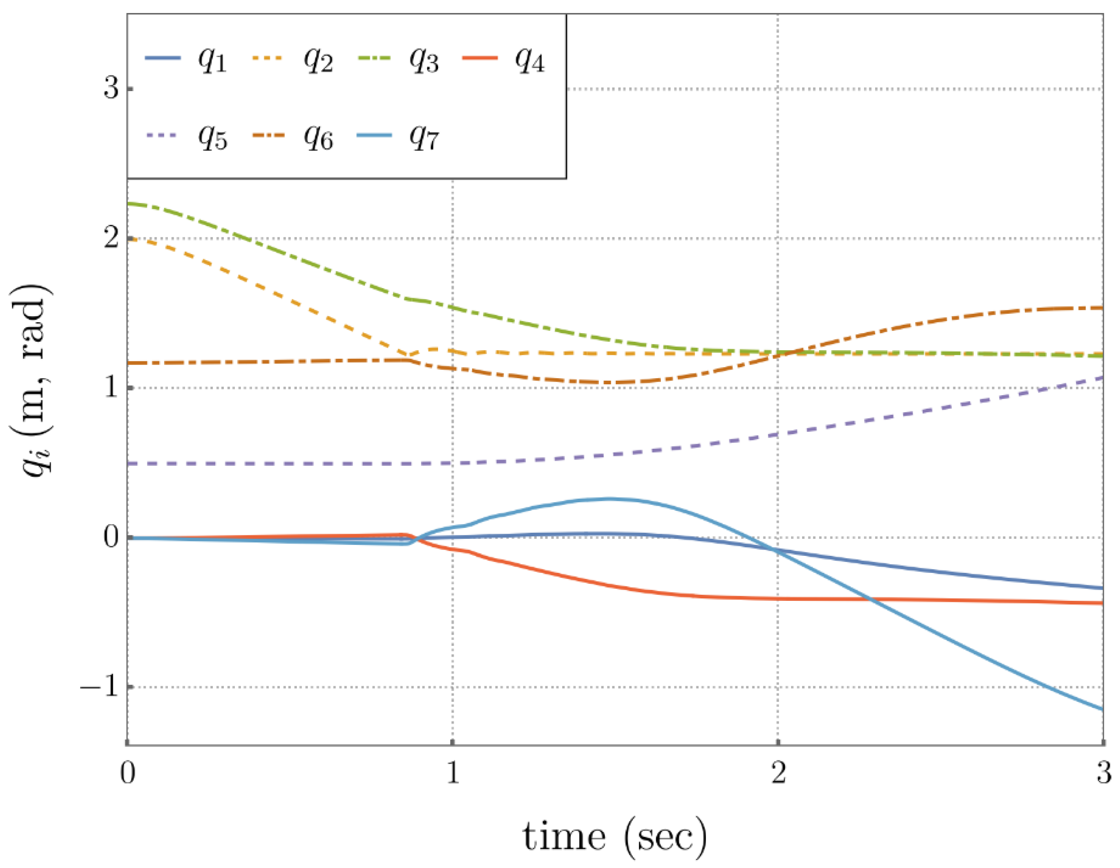
Running this simple second order integrator for three seconds yields results shown in Figures 5.1 and 5.2. Each image in Figure 5.1 depicts the manipulator configuration at a specific time. The images occur at regular intervals, with the earliest images fading away; i.e., becoming more transparent. Figure 5.2 displays generalized coordinates over the three second interval. Comparable results could be obtained by solving Eq. (4.23) for and using to recover .
Figure 5.1.
Composite Rendering of Manipulator Configurations at Specific Times.
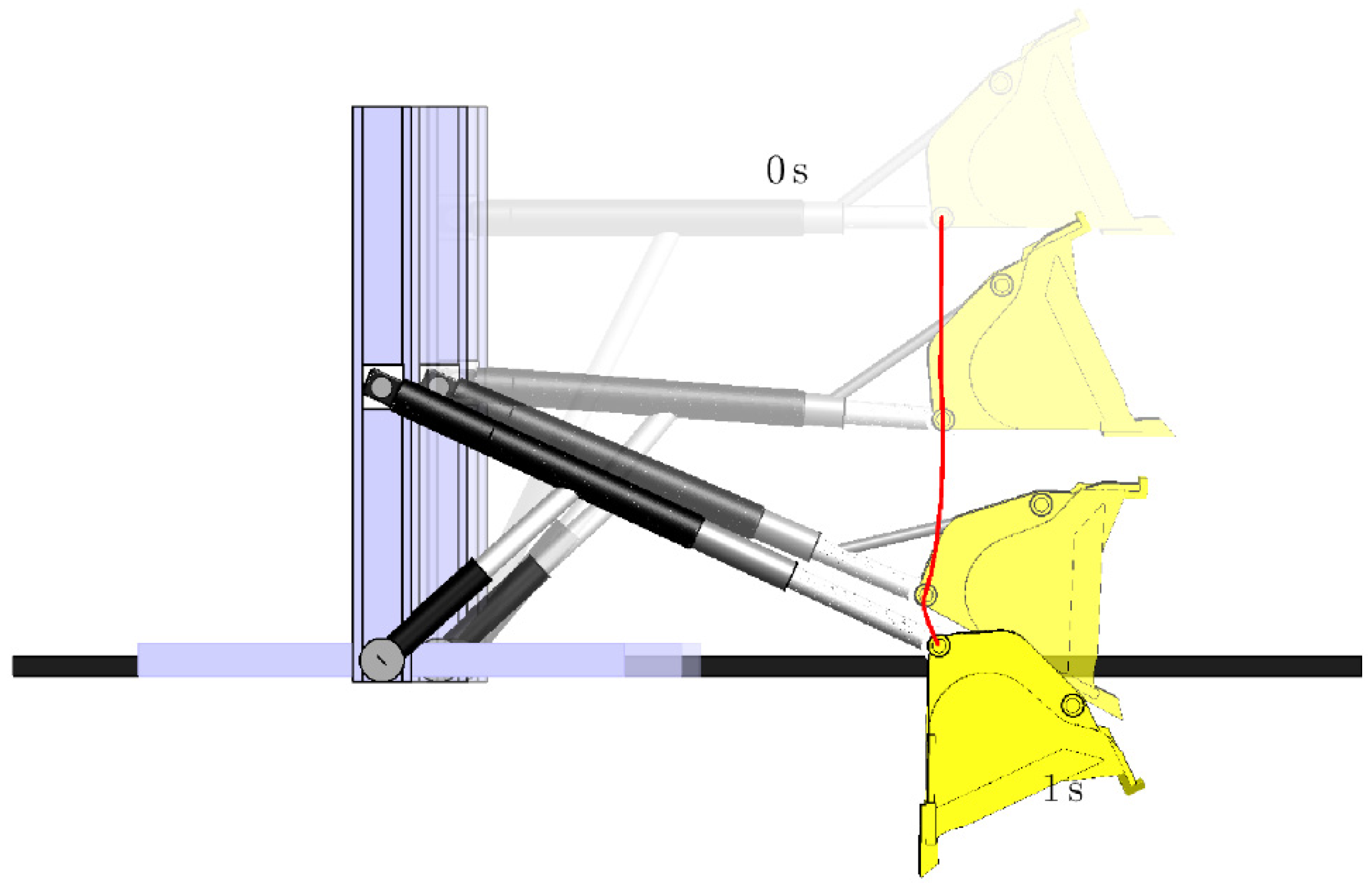
Figure 5.2.
Time Histories of Generalized Coordinates, Representing Free-Fall of the Manipulator Under Gravity, Using Input Space Dynamics.
Figure 5.2.
Time Histories of Generalized Coordinates, Representing Free-Fall of the Manipulator Under Gravity, Using Input Space Dynamics.
The operational space equation of motion of Eq. (4.35) is
This represents a set of ODE. With the same initial conditions and integration procedure [10]
where the acceleration is computed in extended operational space coordinates and transformed to generalized accelerations, for comparison with the foregoing input space integration results.
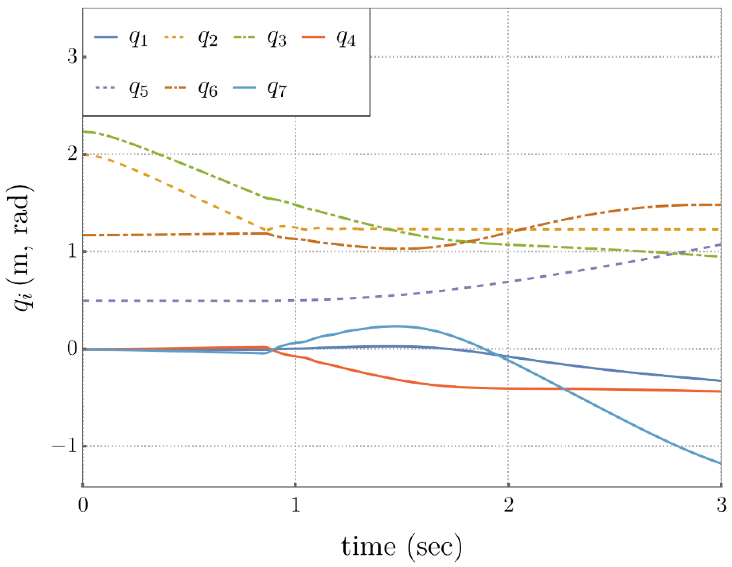
Running this simple second order integrator for three seconds yields results shown in Figure 5.3. The results are essentially identical to the input space results, demonstrating equivalence of input space and extended operational space dynamics.
Figure 5.3.
Time Histories of Generalized Coordinates, Representing Free-Fall of the Manipulator Under Gravity, Using Extended Operational Space Dynamics.
Figure 5.3.
Time Histories of Generalized Coordinates, Representing Free-Fall of the Manipulator Under Gravity, Using Extended Operational Space Dynamics.
5.2. Tracking Task Trajectory, with Kinetic Energy Minimization and Joint Limit Avoidance
Two operational space controllers will be compared in tracking a desired task trajectory zd. For both traditional and extended operational space control, initial conditions of the manipulator are
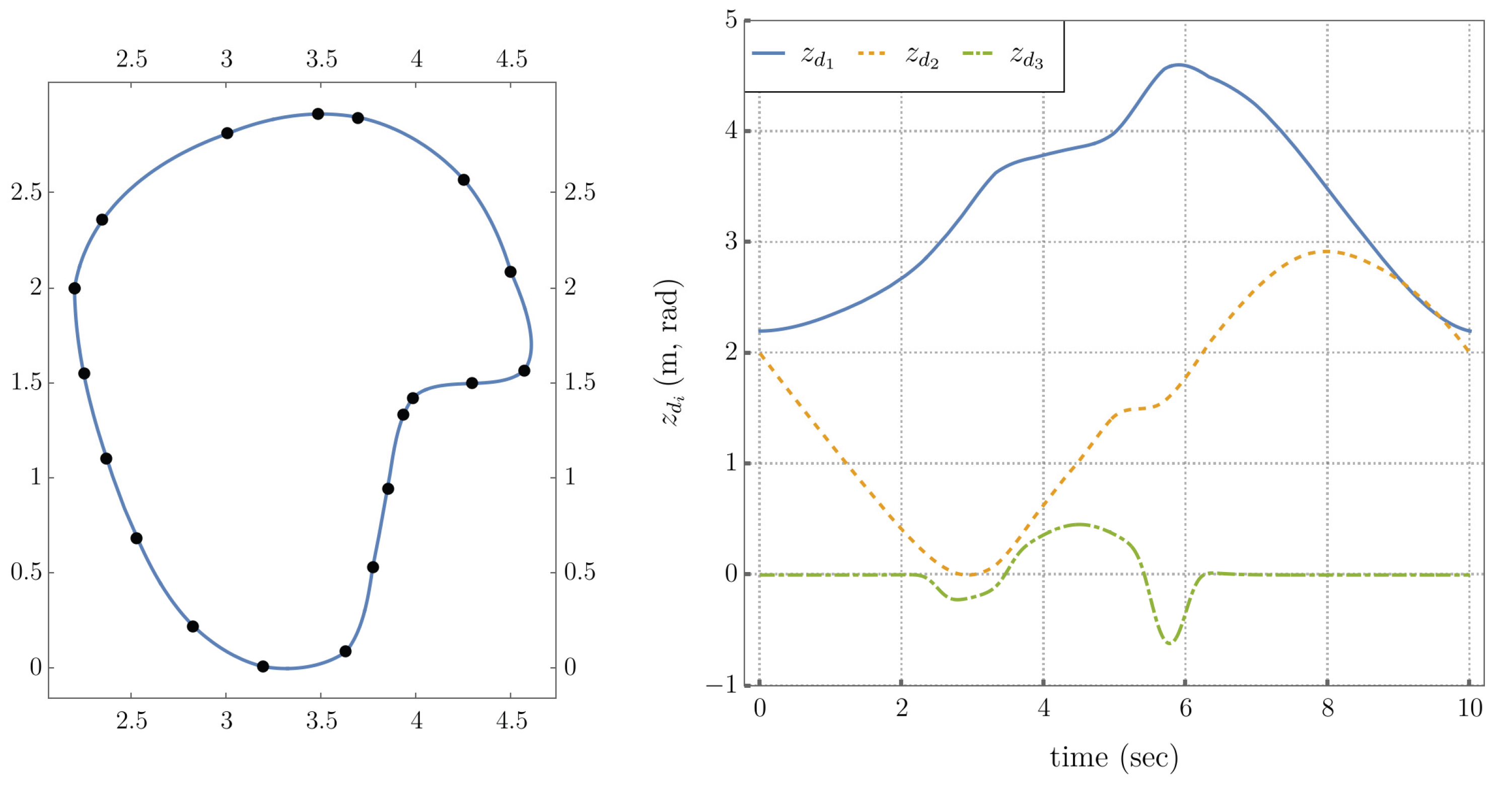
The desired task trajectory is shown in the left of Figure 5.4, with output coordinate time histories on the right.
Figure 5.4.
Desired Reference Signals for Task and Self-Motion Tracking of Traditional and Extended Operational Space Controllers. (Left) Planar Trajectory Passing Through a Set of Points. (Right) Task Output Coordinates.
Figure 5.4.
Desired Reference Signals for Task and Self-Motion Tracking of Traditional and Extended Operational Space Controllers. (Left) Planar Trajectory Passing Through a Set of Points. (Right) Task Output Coordinates.
5.2.1. Traditional Operational Space Control
The multiplier form of the constrained operational space equations is restated from Eq. (2.17),
where terms are defined in Eqs. (2.18) thru (2.24). These equations need to be complemented by the passivity condition on the unactuated joints [8],
where is the selection matrix that specifies the unactuated joints. For example, in this case,
which indicates that the 4th and 7th generalized coordinates are unactuated.
The control input to the plant is then
where
Joint limit avoidance forces , modeled using exponential springs, are specified. These forces are filtered through the null space projection matrix to ensure that they are dynamically decoupled from the task control. Additionally, a kinetic energy minimization term is added.
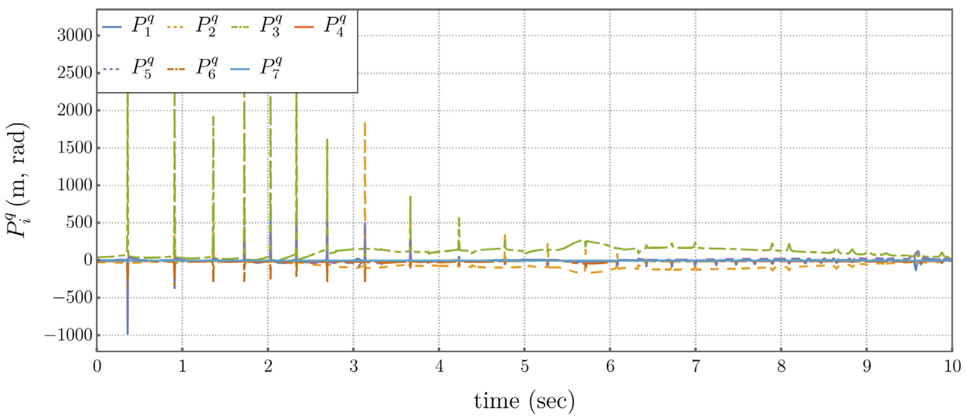
Application of this controller generates the results shown in Figures 5.5 through 5.8. Each image in Figure 5.5 depicts the manipulator configuration at a specific time. The high frequency artifacts in Figures 5.7 and 5.8 are due to joint limits repeatedly being hit.
Figure 5.5.
Snapshots of System Configuration.
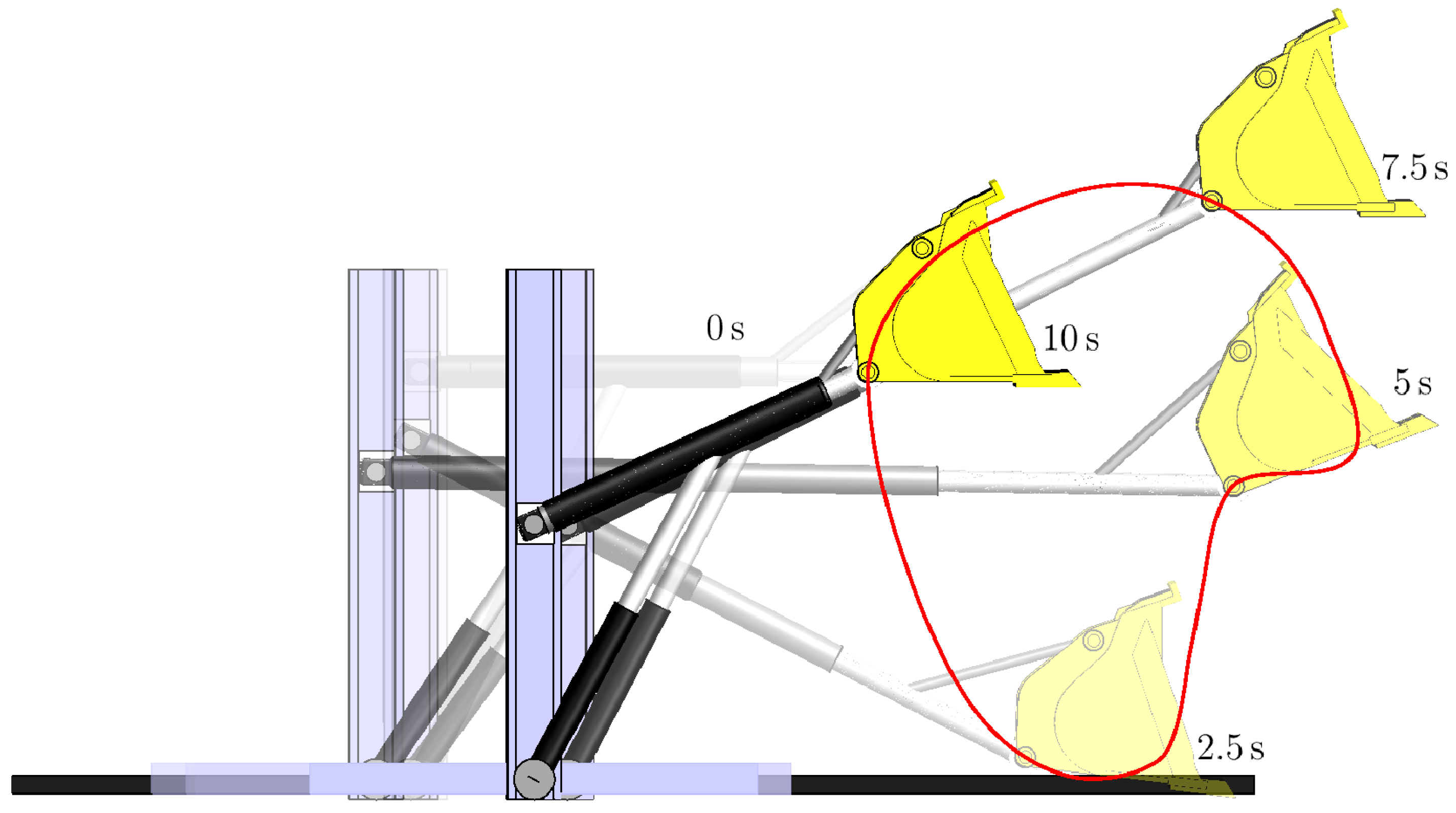
Figure 5.6.
Operational Space Trajectory Using the Traditional Operational Space Controller.
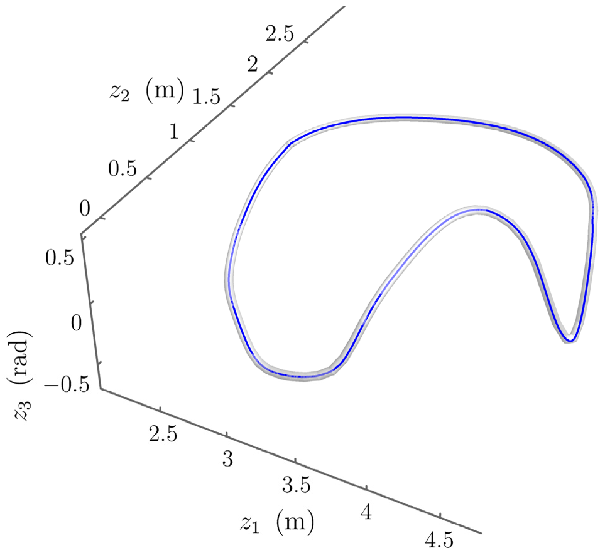
Figure 5.7.
Time Histories 0f Generalized Coordinates Using the Traditional Operational Space Controller.
Figure 5.7.
Time Histories 0f Generalized Coordinates Using the Traditional Operational Space Controller.
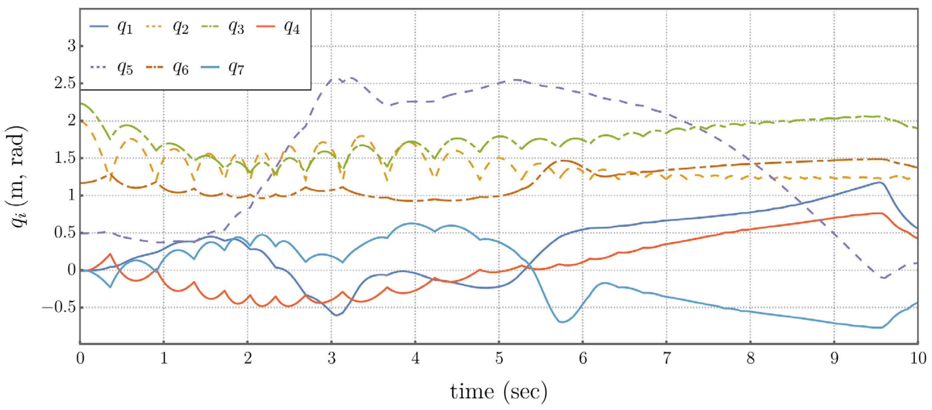
Figure 5.8.
Time Histories of Generalized Forces Under Traditional Operational Space Control.
5.2.2. Extended Operational Space Control
The compound extended operational space equations are restated from Eq. (4.35) as . The control input to the plant is then
where
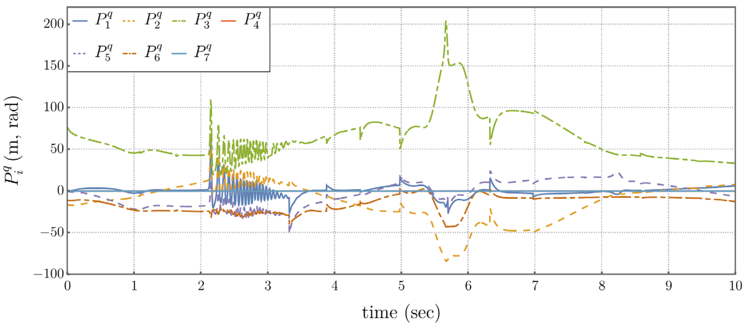
The same joint limit avoidance forces and kinetic energy minimization forces are applied as in the previous example. Application of this controller generates results shown in Figures 5.9 through 5.11, indicating that high frequency artifacts are not present (or are significantly reduced).
Figure 5.9.
Snapshots of System Configuration.
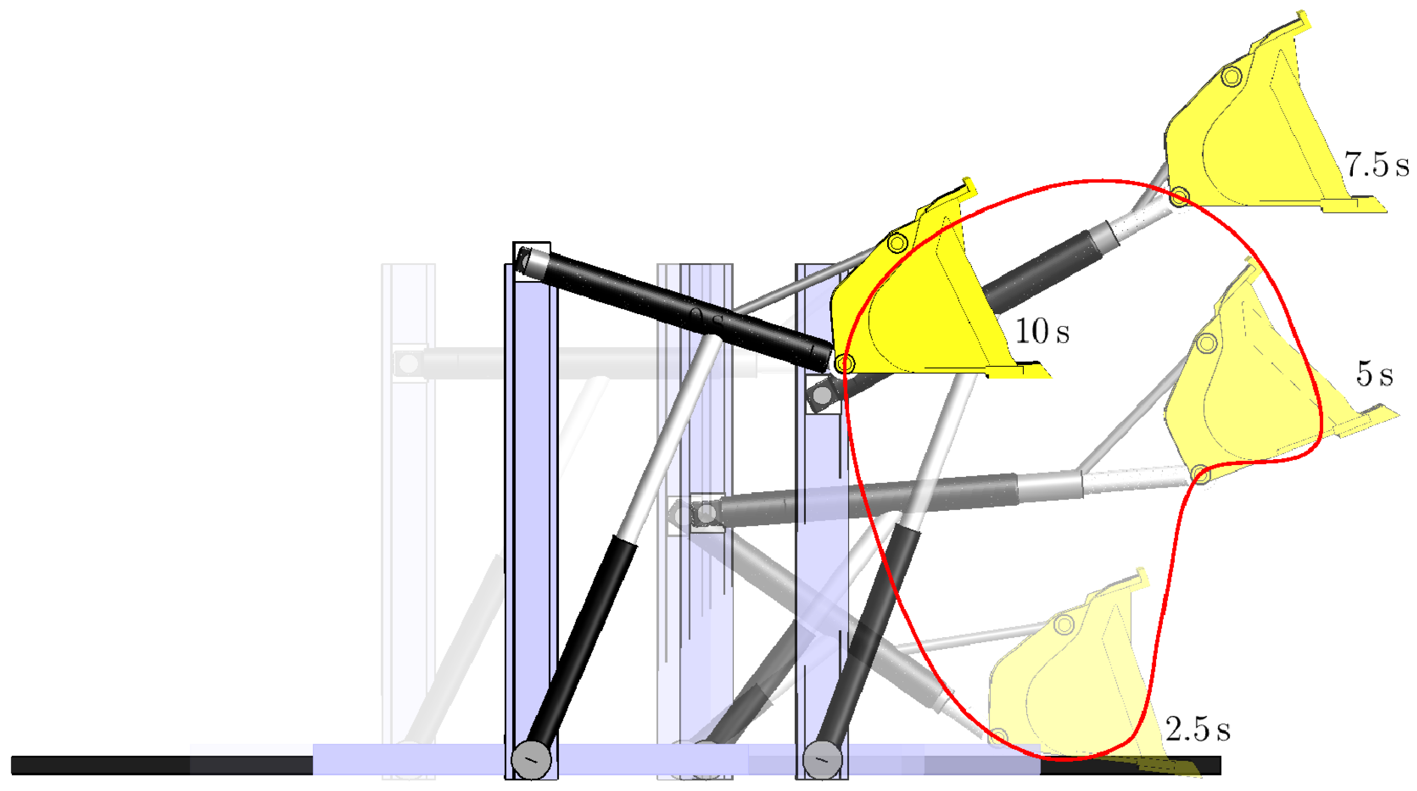
Figure 5.10.
Time Histories of Generalized Coordinates, Using the Extended Operational Space Control, Showing that High Frequency Artifacts Are Not Present.
Figure 5.10.
Time Histories of Generalized Coordinates, Using the Extended Operational Space Control, Showing that High Frequency Artifacts Are Not Present.
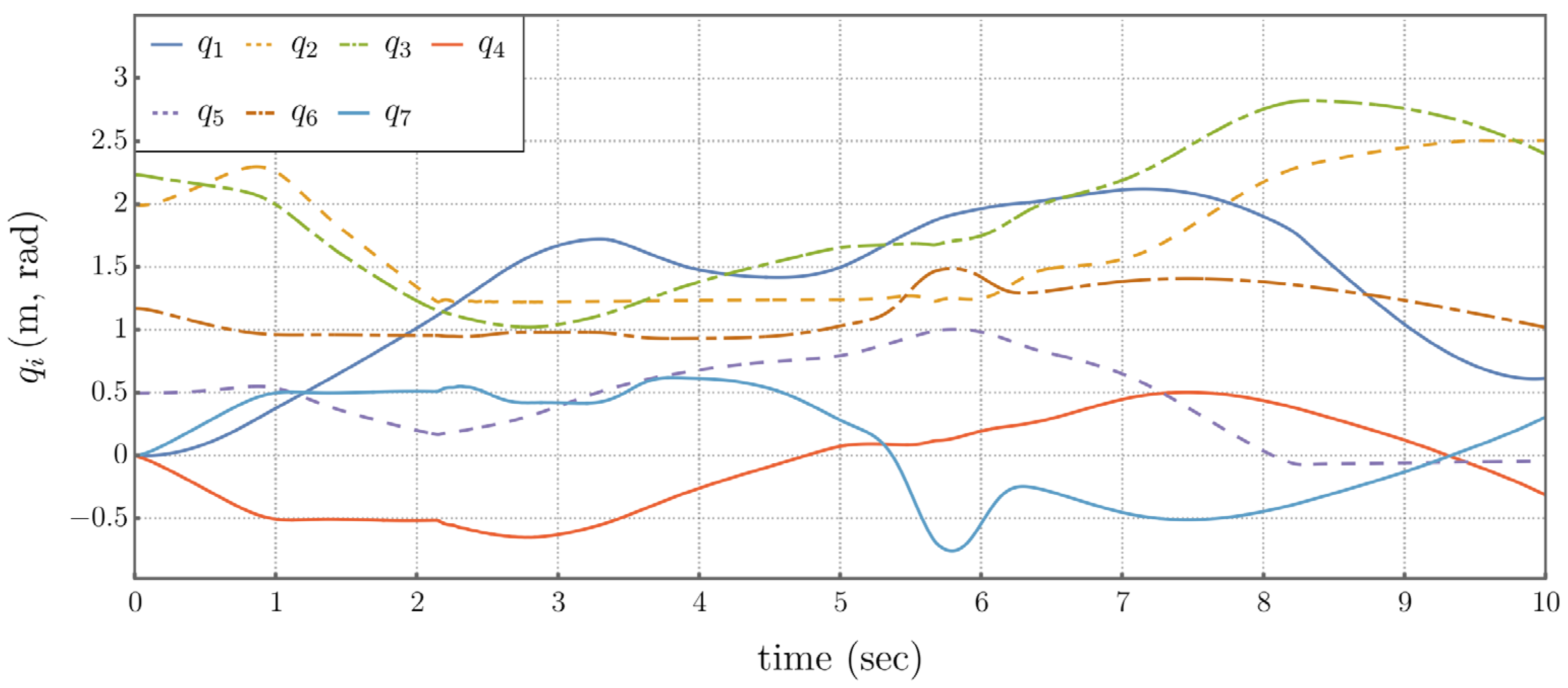
Figure 5.11.
Time Histories of Generalized Forces, Using the Extended Operational Space Controller, Showing that Limited High Frequency Artifacts Are Present.
Figure 5.11.
Time Histories of Generalized Forces, Using the Extended Operational Space Controller, Showing that Limited High Frequency Artifacts Are Present.
5.3. Comparison of Performance Metrics
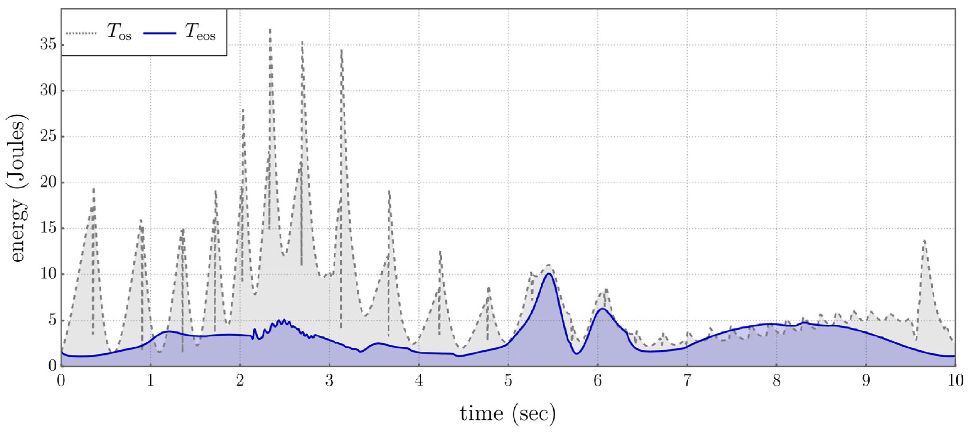
A number of performance metrics have been implemented to establish an objective comparison between the extended operational space control formulation presented herein and the traditional operational space control approaches [11]. These metrics include the kinetic energy, defined as
and plotted in Figure 5.12, showing a significantly greater system kinetic energy throughout the entire time history in the traditional operational space controller, compared to the small stable stored kinetic energy in the extended operational space controller.
Figure 5.12.
Stored Kinetic Energy of the System.
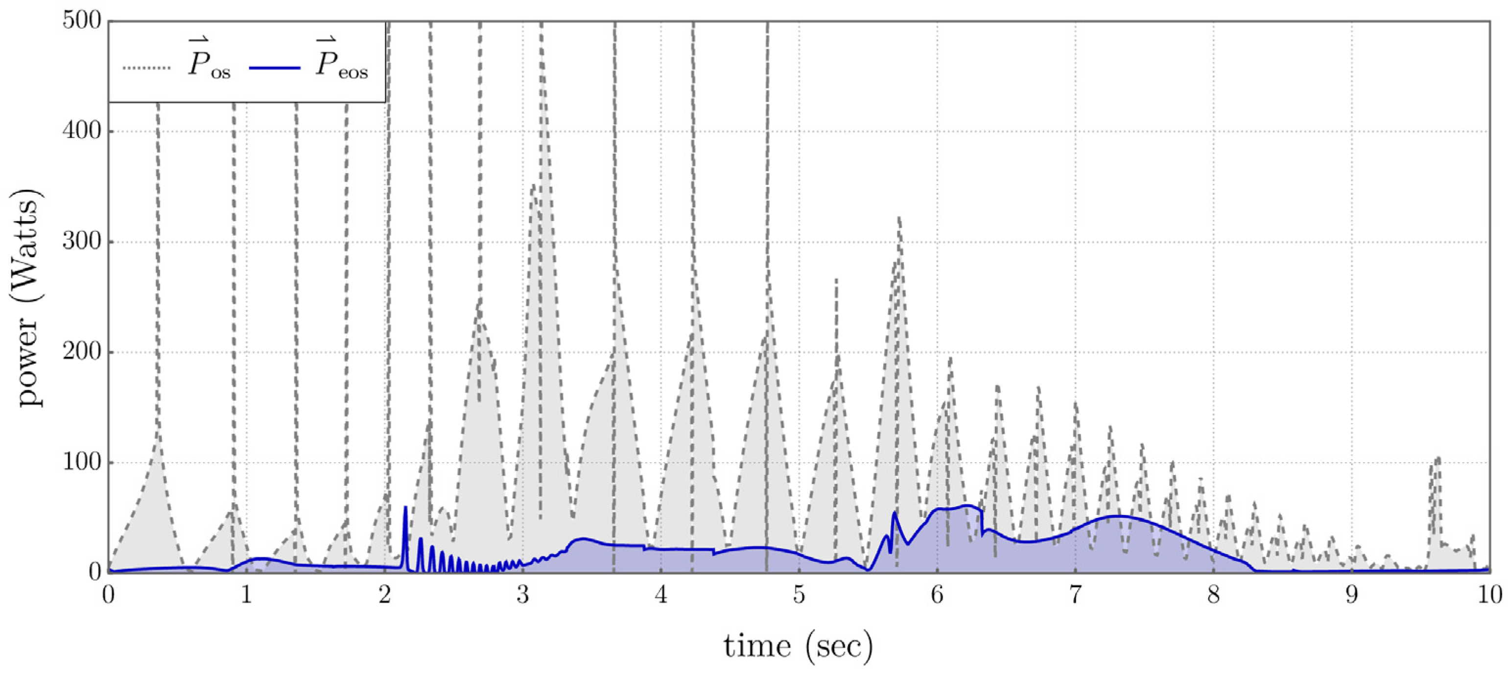
Power is the product of input space force and input space velocity. If this product is positive the flow of power is from actuator to joint, and joint to actuator if the product is negative. If the actuator is perfectly regenerative then all power flowing to it from the joint is recovered. Actuators that are not regenerative will be considered, in which case the power is given by
The plot of Figure 5.13 shows significantly greater system power generated by the actuators throughout the entire time history in the traditional operational space controller, compared with the small stable power generated in the extended operational space controller.
Figure 5.13.
Power Generation for the System.
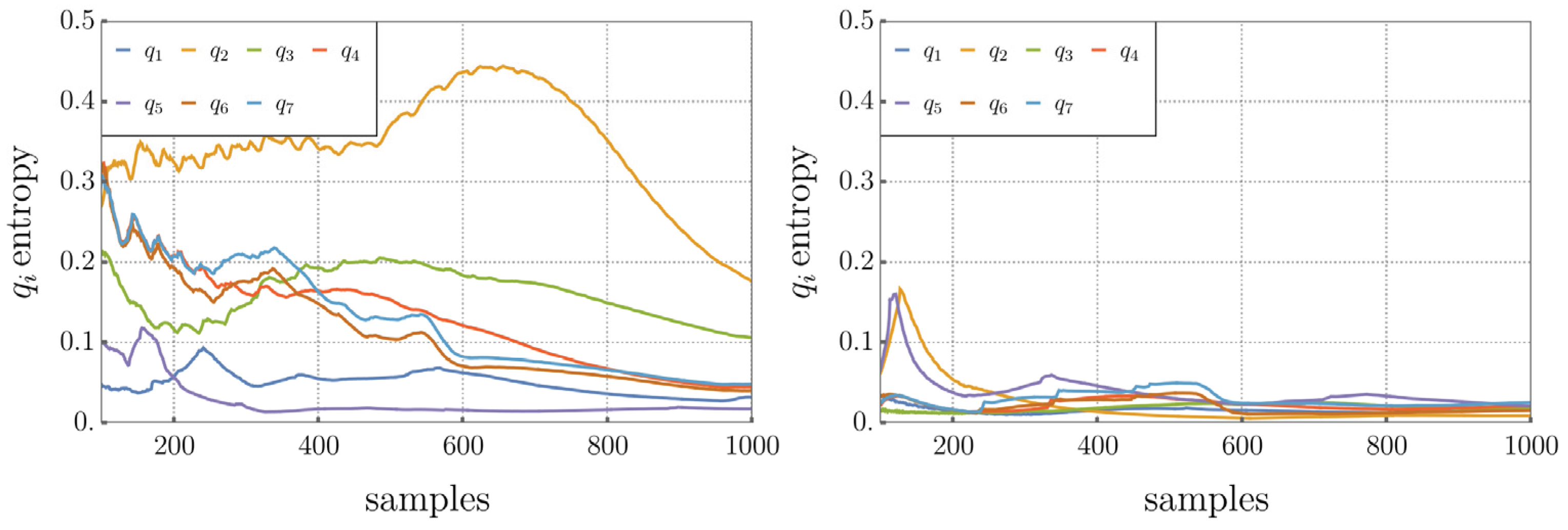
Sample entropy is a measure of complexity [11]. It is used here to characterize the disorder of the internal motion of the manipulator under different control approaches. Sample entropy has been used in biomedical applications and biomechanical research, for example to evaluate postural control [16]. Given a continuous time series over the interval , the discrete time series is defined as
where is the number of time samples. The sample entropy is given by the numerical procedure , where is the embedding dimension that is usually taken to be equal to 2. The term mis the tolerance, usually taken to be equal to , where is the standard deviation of the time series samples. The cumulative entropy of the time series is
For the input space time series ,
As shown in Figure 5.14, a higher general level of entropy, reflecting higher disorder, occurs in the traditional operational space controller (left) compared to the lower entropy in the extended operational space controller (right).
Figure 5.14.
Sample Entropy Computed on Cumulative Sampling (1000 Total Samples Per Signal, Minimum of 100 Samples).
Figure 5.14.
Sample Entropy Computed on Cumulative Sampling (1000 Total Samples Per Signal, Minimum of 100 Samples).
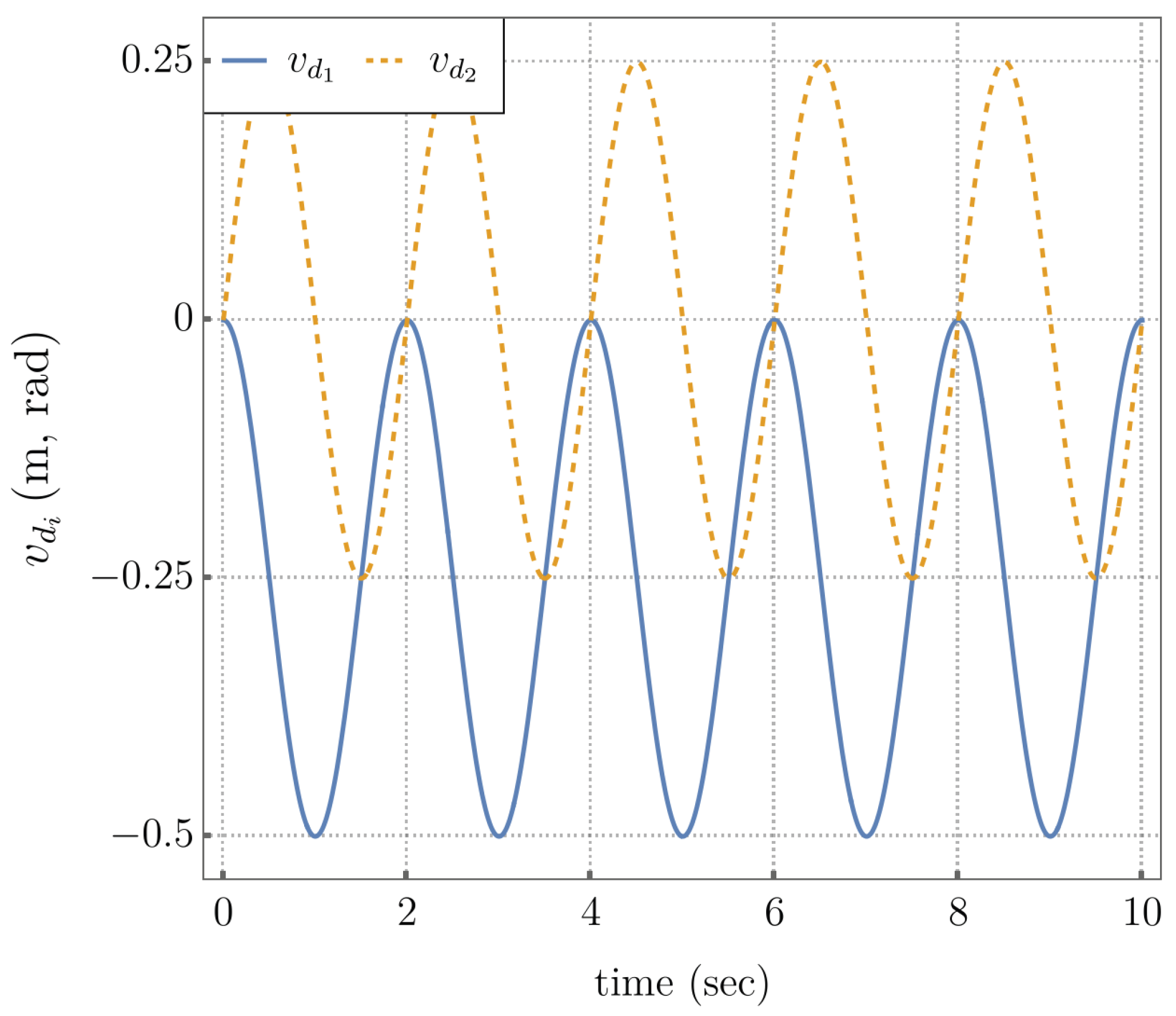
5.4. Self Motion Coordinate Tracking
Self-motion coordinate tracking, in addition to task coordinate tracking, is next demonstrated. The reference trajectories used are shown in Figure 5.15. Note that these are used only for extended operational space control, since traditional operational space control does not allow control of self-motion coordinates. Initial conditions are and .
The compound extended operational space equations are restated from Eq. (4.35) as . The control input to the plant is then
Where .
Figure 5.15.
Self Motion Output Coordinates.
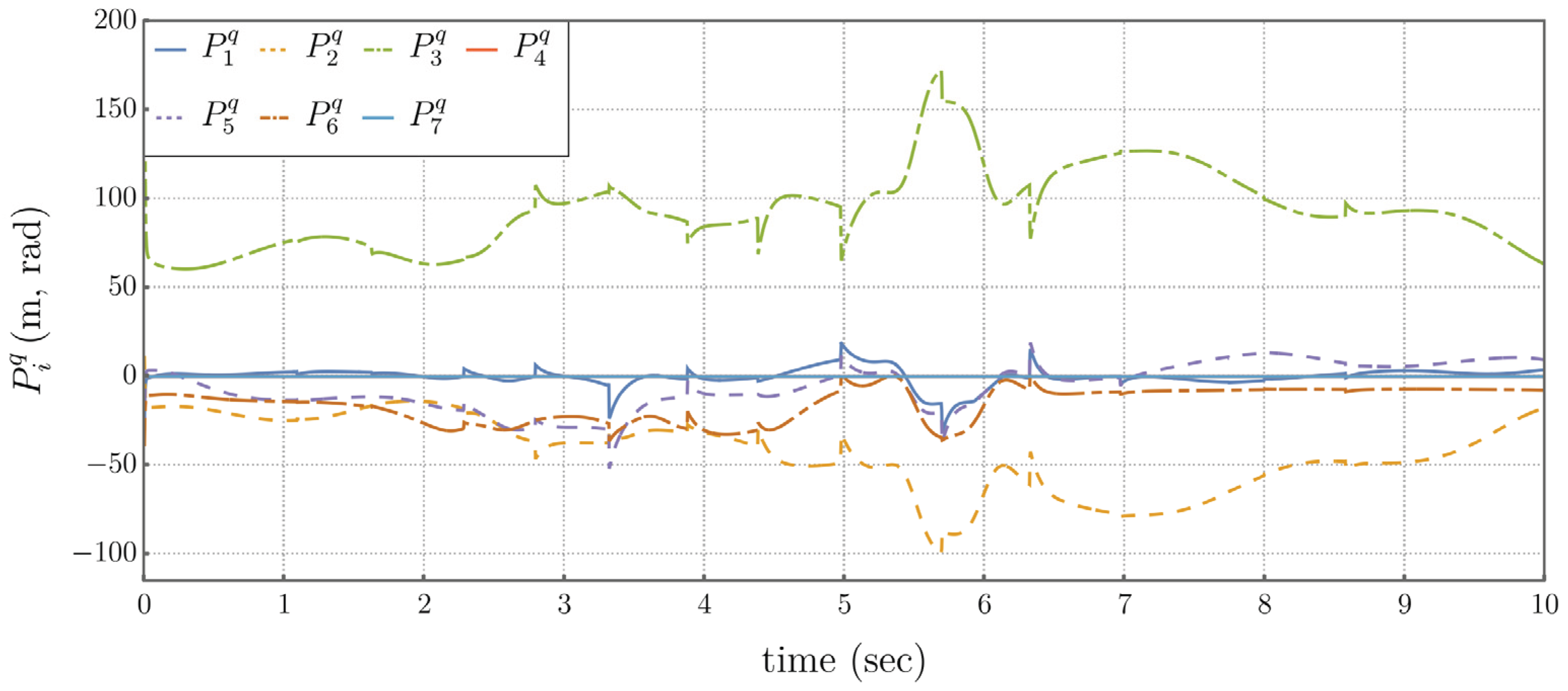
The same joint limit avoidance forces and kinetic energy minimization forces are applied as in previous example. Application of this controller generates results shown in Figures 5.16 through 5.19, indicating tracking of the self-motion coordinates.
Figure 5.16.
Snapshots of System Configuration.
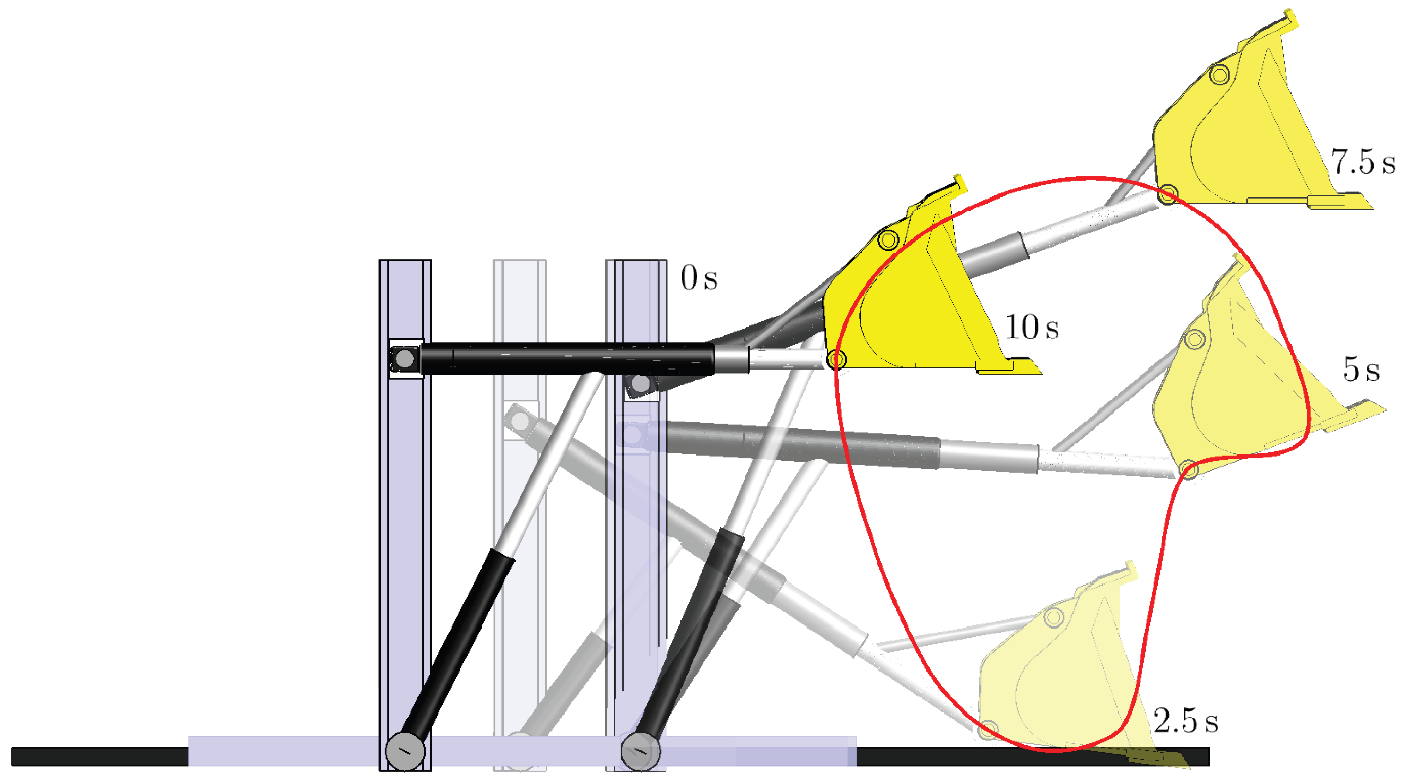
Figure 5.17.
Control Results Using the Extended Operational Space Controller, With Cyclic Evolution of the Self-Motion Coordinates.
Figure 5.17.
Control Results Using the Extended Operational Space Controller, With Cyclic Evolution of the Self-Motion Coordinates.
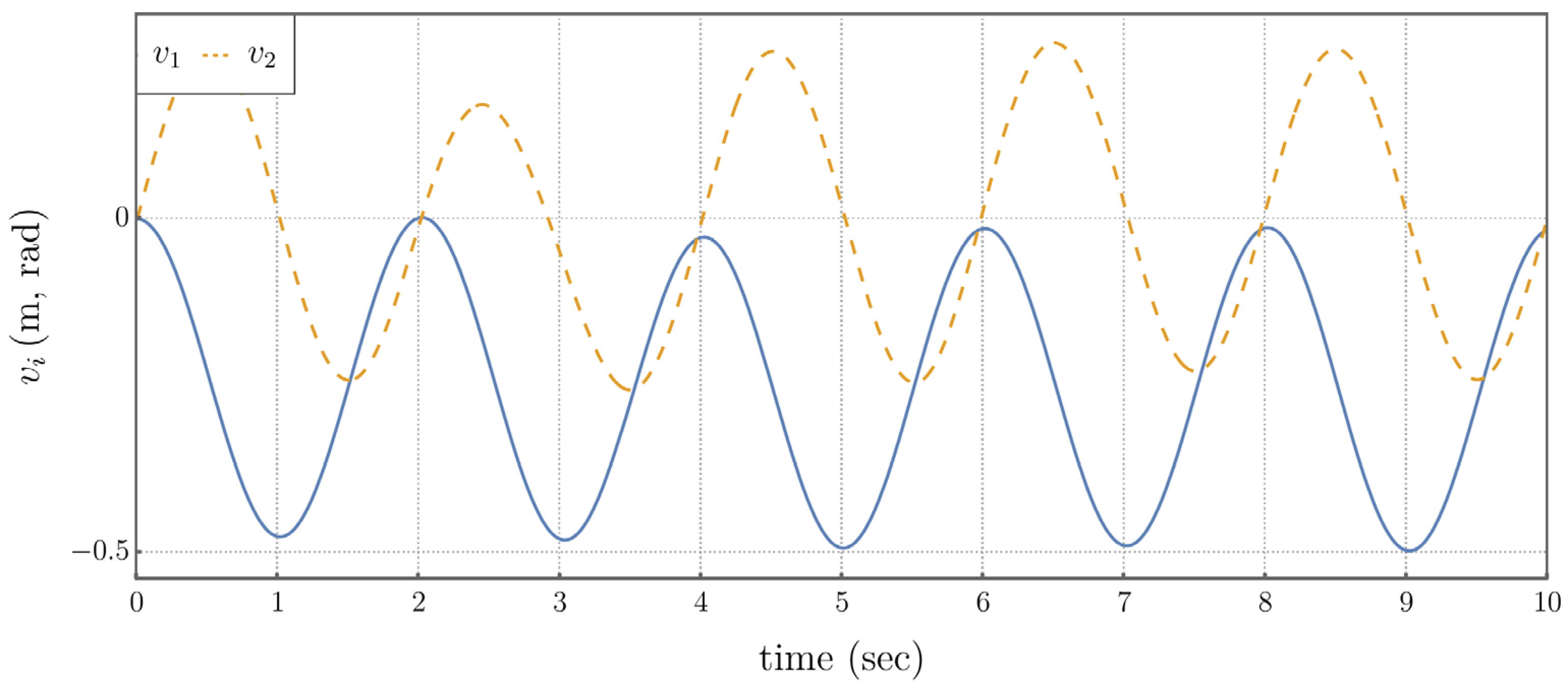
Figure 5.18.
Time Histories of Generalized Coordinates, Using the Extended Operational Space Controller.
Figure 5.18.
Time Histories of Generalized Coordinates, Using the Extended Operational Space Controller.
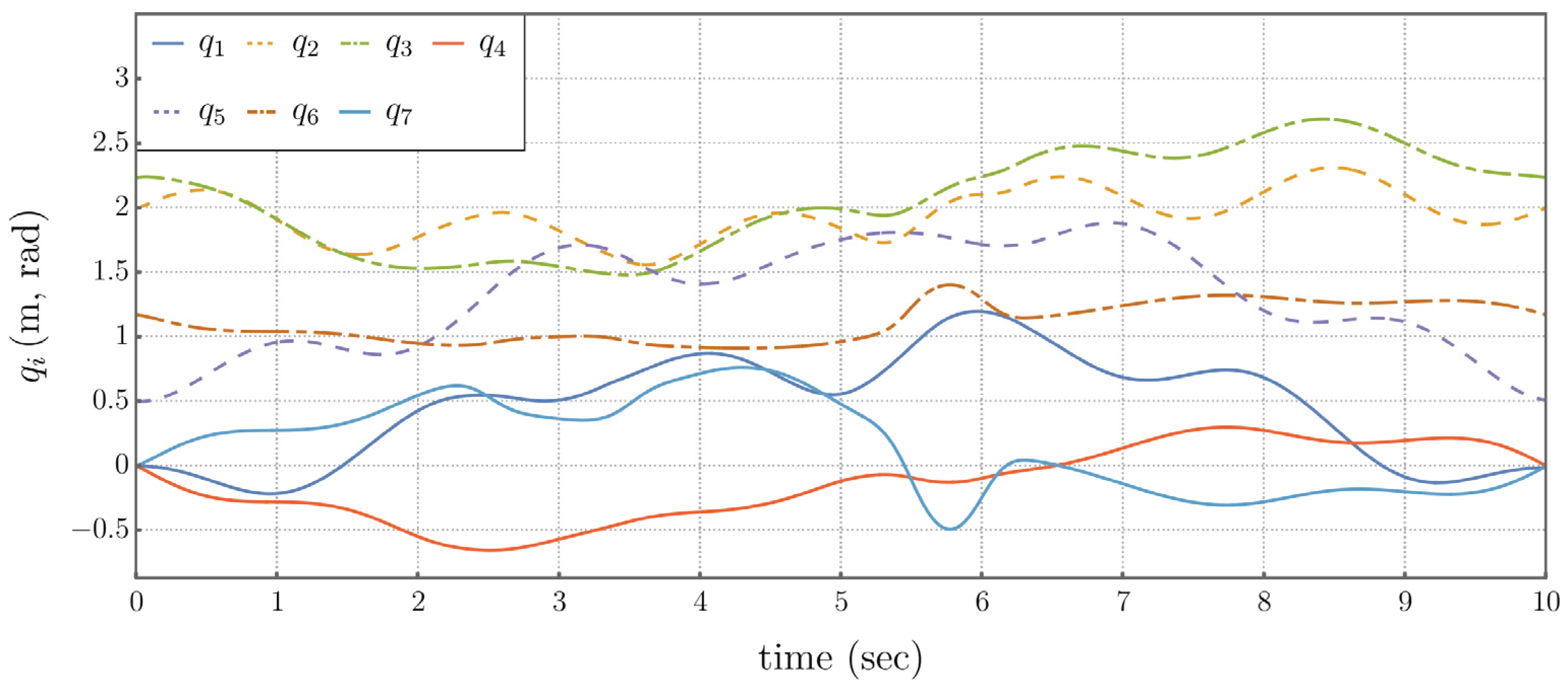
Figure 5.19.
Time Histories of Generalized Forces, Using the Extended Operational Space Controller.
6. Summary and Conclusions
Results from the previous sections have demonstrated the effectiveness of the extended operational space control formulation in tracking both self-motion and task coordinates. Additionally, gradient minimization of kinetic energy has been demonstrated. Most importantly, In the absence of direct specification of self-motion coordinates, the extended operational formulation achieved lower kinetic energy, power consumption, and sample entropy than the traditional operational space formulation.
It is important to note that a dynamically consistent generalized inverse of the task Jacobian for a serial manipulator is defined [10,12,20] to minimize kinetic energy of the solution of the velocity kinematic equation. In fact, the dynamically consistent inverse has the property of yielding the least velocity norm solution. The mass-weighted inverse solution of the velocity equation is precisely the least kinetic energy (analogous to least norm). Despite this property of the dynamically consistent inverse, it can be seen in Figure 5.13 that control based on dynamic consistency does not produce minimal kinetic energy over a time serie, for either serial or compound manipulators. As discussed in [20] for serial manipulators, it should not be expected to do so, since the kinetic energy property that it satisfies is an instantaneous one that is dependent upon the specific configuration.
An area for future investigation will be to establish global properties for the extended operational control formulation, based on analysis of the differential geometry of self-motion manifolds. For example, Hertz’s principle of least curvature [10] reveals that under certain conditions, motion on the constraint manifold is restricted to geodesic (straightest) paths. Without specification of explicit control for the self-motion space, the manner in which the extended operational space approach implicitly controls self-motion is worthy of future investigation.
Author Contributions.
EH and VD conceived and designed the study. EH developed the differential geometry results. VD developed the control results. Eh and VD wrote the article.
Financial Support
This research received no specific grant from any funding agency, commercial or not-for-profit sectors.
Data Availability Statement
The original contributions presented in this study are included in the article and supplementary material.
Conflicts of Interest
The authors declare no conflicts of interest exist.
References
- Atkinson, K. E., 1989, An Introduction to Numerical Analysis, 2nd Ed., Wiley, New York.
- Baumgarte, J. Stabilization of constraints and integrals of motion in dynamical systems. Computer methods in applied mechanics and engineering 1972, 1(1), 1–16. [Google Scholar] [CrossRef]
- Burdick, J. W., 1989, On the Inverse Kinematics of Redundant Manipulators: Characterization of the Self-Motion Manifolds, Proceedings, 1989 IEEE Int. Conf. Robot Automation, Scottsdale AZ, pp264-270. [CrossRef]
- Chiaverini, S., Oriolo, G., and Maciejewski, A. A., 2016, Redundant Robots, Siciliano and Khatib eds, Springer Handbook of Robotics, 2nd ed, Springer-Verlag Berlin.
- Conconi, M.; Carricato, M. A new assessment of singularities of parallel kinematic chains. IEEE Transactions on Robotics 2009, 25, 757–770. [Google Scholar] [CrossRef]
- Corwin, L. J.; Szczarba, R. H. Multivariable Calculus; Marcel Dekker: New York, 1982. [Google Scholar]
- De Luca, A.; Oriolo, G. Nonholonomic Behavior in Redundant Robots Under Kinematic Control. IEEE Transactions on Robotics and Automation 1997, 13, 776–782. [Google Scholar] [CrossRef]
- De Sapio, V.; Khatib, O.; Delp, S. Task-level approaches for the control of constrained multibody systems. Multibody Sys. Dyn. 2006, 16, 73–102. [Google Scholar] [CrossRef]
- De Sapio, V.; Park, J. Multitask constrained motion control using a mass- weighted orthogonal decomposition. Journal of Applied Mechanics 2010, 7, 041004. [Google Scholar] [CrossRef]
- De Sapio, V. Advanced analytical dynamics: theory and applications; Cambridge University Press, 2017. [Google Scholar]
- Delgado-Bonal, A.; Marshak, A. Approximate Entropy and Sample Entropy: A Comprehensive Tutorial. Entropy 2019, 21, 541. [Google Scholar] [CrossRef] [PubMed]
- Drucker, S.; Seifried, R. Trajectory-tracking control from a multibody system dynamics perspective. Multibody Sys. Dyn. 2023, 38, 341–363. [Google Scholar] [CrossRef]
- Goldstein, H. Classical Mechanics, 2nd ed.; Addison-Wesley: Reading, Mass, 1980. [Google Scholar]
- Gosselin, C.; Schreiber, L.-T. Kinematically Redundant Spatial Parallel Mechanisms for Singularity Avoidance and Large Orientational Workspace. IEEE Transactions on Robotics 2016, 32, 286–300. [Google Scholar] [CrossRef]
- Gosselin, C.; Schreiber, L.-T. Redundancy in Parallel Mechanisms: A Review. Applied Mechanics Reviews 2018, 70, 010802. [Google Scholar] [CrossRef]
- Hadamus, A.; Białoszewski, D.; Błażkiewicz, M.; Kowalska, A. J.; Urbaniak, E.; Wydra, K.T.; Wiaderna, K.; Boratyński, R.; Kobza, A.; Marczyński, W. Assessment of the Effectiveness of Rehabilitation after Total Knee Replacement Surgery Using Sample Entropy and Classical Measures of Body Balance. Entropy 2021, 23, 164. [Google Scholar] [CrossRef] [PubMed]
- Haug, E. J. Redundant Non-Serial Implicit Manipulator Kinematics and Dynamics. Journal of Mechanisms and Robotics 2024, 16, 061017. [Google Scholar] [CrossRef]
- Haug, E. J. Redundant Non-Serial Compound Manipulator Kinematics and Dynamics. Mechanism and Machine Theory 2024, 200, 105717. [Google Scholar] [CrossRef]
- Haug, E. J. A Cyclic Differentiable Manifold Representation of Redundant Manipulator Kinematics. Journal of Mechanisms and Robotics 2024c, 16, 061005. [Google Scholar] [CrossRef]
- Haug, E. J.; De Sapio, V.; Peidro, A. Extended Operational Space Kinematics, Dynamics, and Control of Redundant Serial Manipulators. Robotics 2024, 13, 170. [Google Scholar] [CrossRef]
- Haug, E. J. Computer-Aided Kinematics and Dynamics of Mechanical Systems. In Modern Methods; Springer: Cham, Switzerland, 2026. [Google Scholar]
- Jain, A. Operational Space Inertia for Closed-Chain Robotic Systems. Journal of Computational and Nonlinear Dynamics 2014, 9, 021015. [Google Scholar] [CrossRef]
- Khatib, O. A Unified Approach for Motion and Force Control of Robot Manipulators: The Operational Space Formulation”. IEEE J of Robotics and Automation 1987, RA-3, 43–53. [Google Scholar] [CrossRef]
- Khatib, O. The Operational Space Framework. JSME International Journal, Series C 1993, 36, 277–287. [Google Scholar] [CrossRef]
- Lee, J.M. Introduction to Smooth Manifolds, 2nd ed.; Springer: New York, 2013. [Google Scholar]
- Luces, M.; Mills, J. K.; Benhabib, B. A Review of Redundant Parallel Kinematic Manipulators. J. Intel Robot Sys 2017, 86, 175–198. [Google Scholar] [CrossRef]
- Mendelson, B. Introduction to Topology; Allyn and Bacon: Boston, 1962. [Google Scholar]
- Pars, L. A. A Treatise on Analytical Dynamics; Reprint by Ox Bow Press (1979): Woodbridge, Conn, 1965. [Google Scholar]
- Robbin, J. W.; Salamon, D. A. Introduction to Differential Geometry; Springer: Berlin, 2022. [Google Scholar]
- Sadeghian, H., Keshmiri, M., Villani, L., and Siciliano, B., 2012, Priority Oriented Adaptive Control of Kinematically Redundant Manipulators, IEEE International Conference on Robotics and Automation, Saint Paul, Minnesota, May 14-18, 2012, pp. 293-298. [CrossRef]
- Shamir, T.; Yomdin, Y. Repeatability of Redundant Manipulators: Mathematical Solution of the Problem. IEEE Transactions on Automatic Control 1988, 33, 1004–1009. [Google Scholar] [CrossRef]
- Strang, G. Liner Algebra and its Applications, 2nd ed.; Academic Press: New York, 1980. [Google Scholar]
- Whitney, D. E. Resolved Motion Rate Control of Manipulators and Human Prostheses. IEEE Transactions on Man-Machine Systems 1969, 10, 47–53. [Google Scholar] [CrossRef]
Disclaimer/Publisher’s Note: The statements, opinions and data contained in all publications are solely those of the individual author(s) and contributor(s) and not of MDPI and/or the editor(s). MDPI and/or the editor(s) disclaim responsibility for any injury to people or property resulting from any ideas, methods, instructions or products referred to in the content. |
© 2025 by the authors. Licensee MDPI, Basel, Switzerland. This article is an open access article distributed under the terms and conditions of the Creative Commons Attribution (CC BY) license (http://creativecommons.org/licenses/by/4.0/).
Copyright: This open access article is published under a Creative Commons CC BY 4.0 license, which permit the free download, distribution, and reuse, provided that the author and preprint are cited in any reuse.


