
Submitted:
01 December 2025
Posted:
02 December 2025
You are already at the latest version
Abstract
Helicopter vibration is an inherent characteristic of rotorcraft operations arising from transmission dynamics and unsteady aerodynamic loading, posing challenges to flight control and longevity of structural components. Excessive vibration elevates pilot workload and accelerates fatigue damage in critical components. Leveraging advances in optimal control and microelectronics, the active vibration control methods offer superior adaptability compared to the passive techniques limited by added weight and narrow bandwidth. In this study, a comprehensive vibration analysis and optimal control framework are developed for the Bo 105 helicopter rotor blade exhibiting flapping, lead–lag, and torsional (triply coupled) motions, where a Linear Quadratic Regulator (LQR) is employed to suppress vibratory responses. An analytical formulation is constructed to estimate the blade’s sectional properties and are used to compute the coupled natural frequencies of vibration by modified Galerkin method. An orthogonality condition for the coupled flap–lag–torsion dynamics is established to derive the corresponding state-space equations for both hovering and forward-flight conditions. The LQR controller is tuned through systematic variation of the weighting parameter Q, revealing an optimal range of 102−104 that balances vibration attenuation and control responsiveness. The predicted frequencies of the vibrating rotor blade are compared with the finite element modeling results and published experimental data. The proposed framework illustrates the underlying dynamics of the triply coupled rotor-blade’s vibration, demonstrates modal vibration reduction on the order of 60–90%, and provides a theoretical benchmark for future actuator-integrated and experimental studies.
Keywords:
helicopter rotor blade
; vibration control
; modified Galerkin method
; finite element
; composite mechanics
; hovering flight
; forward flight
1. Introduction
Vibration is an inherent phenomenon in all dynamic systems and generally manifests as an oscillatory motion arising from the system’s mass and relative component interactions. Regardless of the system complexity, these oscillations act as disturbances that dissipate energy, reduce efficiency, and shorten service life of the system components [1]. In automotive and aerospace vehicles, vibrations contribute significantly to structural fatigue, acoustic noise, and passenger discomfort, ultimately compromising operational reliability. Therefore, effective vibration control is critical to ensure component durability and optimize system performance. The primary objective of vibration control is to mitigate unwanted oscillations induced either by external disturbances or internal structural imbalances and remains challenging to select the most effective control strategy [2]. In helicopter rotor systems, unlike hovering flight, forward flight introduces asymmetric aerodynamic loading [3] owing to variations in the relative airflow velocity between the advancing and retreating blades. This generates periodic aerodynamic loadings at the blade root leaving residual unbalanced components that excite harmonics near the blade-passing frequency, potentially coupling with structural modes and leading to resonance. To address these challenges, researchers have explored effective control methodologies and actuation systems aimed at achieving vibration suppression at desired levels under diverse operating conditions including unsteady aerodynamics and gust loadings [4].
Previous studies have shown the effort of researchers provided for vibration control using various strategies including the application of smart materials. A finite element model [5] was proposed by Lam et al. [6] for piezoelectric composite laminates, where a velocity feedback control algorithm was used. Chuaqui et al. [7] used the local collocation method based on the finite- difference generated radial basis functions to implement a constant-gain velocity feedback active vibration control for cantilever piezoelectric smart beams. The effective use of composite materials with piezoelectric sensors and actuators attached or embedded between composite layers can also be used to suppress vibrations [8,9,10]. All these studies emphasized the need to understand active vibration control in continuous systems through a combination of analytical modeling, state estimation, and control optimization.
Active vibration control is categorized into higher harmonic control (HHC), individual blade control (IBC), and active control of structural response [11,12]. Among them, HHC and IBC involve control of blade pitch or trailing edge flap deflection to generate unsteady, higher harmonic loads that cancel the original vibration. In HHC, actuators are placed below the swash plate; hence, the mechanically applicable control frequencies are limited to three blades [11]. The IBC is a suitable method to overcome the limitation of the HHC [12]. In IBC, the actuators are attached to the rotating frame based on the same HHC algorithm. As each rotor blade is actuated individually, it provides more flexibility to control undesirable dynamic phenomena and hence, with the passage of time, the design of IBC has evolved more with the emergence of smart materials.
Experimental and numerical studies have further advanced active vibration control techniques demonstrating their effectiveness across rotorcraft and other complex dynamic systems. Park et al. [13] investigated the performance of a lift-offset rotor with IBC and found that the rotor hub vibration for high-speed flight could be reduced significantly with multiple harmonic inputs. Experimental studies involving IBC, promising for helicopter vibration attenuation and gust alleviation are highlighted in the research study conducted by Yang et al. [14]. They showed that under the effect of high harmonic input, the vibratory loads on the rotor hub could be reduced by 65% for forward flights. A wind-tunnel study of two rotors without actuators in the rotating frame in a Mach-scaled model revealed that the IBC had potential to reduce the vibration up to 77% in the descent flight [15]. Following this, full-scale rotor blade analysis was also conducted for the four-bladed Bo 105 helicopter rotor to investigate the IBC system at the NASA Ames Research Center showing simultaneous reduction in vibration and blade–vortex interaction noise [16,17]. Chia et al. [18] extended these efforts by developing the HELINOIR computational framework for predicting and controlling low-frequency rotorcraft noise using active flaps, which was validated against the wind-tunnel results.
To apply the control strategy successfully on the rotor blade, the vibratory load on the rotor blade needs to be properly estimated which depends on the corresponding aerodynamic environment for different flight conditions, coupling among the various degrees-of-freedom (DOFs) of motion of the rotor blade, blade structure, and relevant material properties. To estimate the vibratory response of the rotor blade accurately, the vibration frequencies need to be evaluated precisely. Besides the coupling between bending and torsional vibrations caused by noncoincident inertial and elastic axes in composite rotor blades, different ply orientations in the composite layers of the blade also create additional couplings among various DOFs of motion. Wang et al. [19] studied the vibration characteristics of a composite helicopter rotor blade to investigate the effect of moisture absorption on the vibration characteristics using finite element analysis (FEA). Tian et al. [20] conducted the failure analysis of a composite helicopter rotor blade using the VABS tool to explore the local-global design optimization and presented numerical examples to show the capability of the toolset for designing composite blades. In addition to the coupling among the DOFs of motion of the rotor blade generated from various styles of composite lay-ups, the curved tip of the blade offers extra coupling to influence the frequencies of vibration [21], which has the potential to be used as a morphing concept for regulating the vibration. Taymaz [22] presented an optimization study showing that the structural orientation of composite layers in the rotor blade could significantly affect its vibration characteristics and needed to be considered as an important factor for designing a passive vibration control system. All these studies justify that proper prediction of vibration is crucial for estimating the structural deformation of the rotor blade and utilizing that to design the relevant optimal vibration controller.
To unravel the core vibration dynamics in a triply coupled rotor system, a theoretically transparent yet computationally efficient framework is essential, providing a baseline for the development and validation of more advanced control strategies. Majority of the previous research activities are based on identification of the rotor blade model experimentally, or through finite element simulation having a single DOF of motion or considering the blade as a rigid one. However, a fundamental study based on classical mechanics and mathematical modeling for coupled vibration among multiple DOFs of motion of a flexible rotor blade is essential for comprehending the underlying physics and for attenuating the vibration. To identify the research needs, a mathematical model of vibration for an isolated Bo 105 helicopter rotor blade having coupled, three DOFs of motion are derived in this study. An analytical method is developed to estimate the sectional properties of the rotor blade. The frequencies of vibration are estimated from the modified Galerkin method (MGM) [23] and FEA and compared with experimental results. The quasi-steady-state lift, drag, and torsional moment are considered as principal aerodynamic loadings for both hovering and forward flights. The state-space model of the coupled equations of motion is derived by developing the orthogonality condition for triply coupled DOFs of motion. The IBC technique is implemented to reduce the three DOFs of motion rotor blade vibration. A Linear Quadratic Regulator (LQR) controller is designed based on the derived state-space model using MATLAB (MathWorks, 2024) control system toolbox. The controller is tuned to achieve optimal vibration reduction for all the DOFs of the rotor blade. This actuator-free analysis not only avoids hardware-specific constraints but also provides a benchmark for validating numerical or experimental implementations in future studies.
2. Materials and Methods
2.1. Modeling of the Composite Helicopter Rotor Blade
2.1.1. Physical model: The Bo 105 Helicopter Rotor Blade
The physical model of vibration estimation and control incorporates the Messerschmitt-Bölkow-Blohm Bo 105 helicopter rotor blade as the base model [24]. The Bo 105 helicopter rotor blade is flexible and has three, coupled DOFs of motion–the out-of-plane or the flapping deflection, ; the in-plane or lead-lag deflection, ; and the torsional displacement, of the rotor blade about the elastic axis. A sketch of such a rotor blade is shown in Figure 1(a) with three types of aerodynamic loadings associated with the three aforementioned DOFs of motion–the out-of-plane bending force per unit length, along axis; in-plane bending force per unit length, along axis; and pitching or torsional moment per unit length, about the elastic axis or axis. The distance between the centroidal axis (CA) and the elastic axis is expressed as . The Bo 105 rotor blade is also considered to have a hingeless rotor system which indicates that the root of the rotor blade is fixed securely to the support [24,25]. A typical hingeless rotor system is described in Figure 1(b).
2.1.2. Cross-Sectional Analysis
The proposed cross-section of the rotor blade for free vibration analysis is based on the geometry of the Bo 105 helicopter rotor blade [24] section. Figure 2 describes a proposed Bo 105 rotor blade section composed of a thin, orthotropic fiberglass-epoxy [25], outer composite shell with the fiber volume fraction of 0.6 and a thick, inner composite core composed of an isotropic polymethacrylimide (PMI) foam called Rohacell [25] and an isotropic Honeycomb structure [25]. The profile of the cross section resembles the NACA 23012 airfoil [26]. The composite shell acts as a balanced laminate composed of four plies with a high strength to weight ratio compared to the inner core of the cross-section and can be considered as a sandwich beam. This cross-sectional configuration of the Bo 105 rotor blade is considered uniform throughout its length from blade root to the blade tip. The blade features a hingeless rotor system which can be treated as a cantilever blade having a fixed end at the root [24,25].
Properties of the materials in the composite section in Figure 2 are given in Table 1 and Table 2 [25] where, , , , and indicate the density, major Poisson’s ratio, thickness, and in-plane shear modulus of the composite shell, respectively; and indicate the elastic modulus of the composite shell in the fiber direction and transverse direction, respectively; and and represent the elastic modulus of the isotropic Honeycomb and Rohacell cores, respectively.
The rotor blade can be considered as a long, thin plate so that the plane stress assumptions hold good. However, the curvature effect of the blade section contour must be considered in the analysis. The key part of the cross-sectional analysis is to find the profile of the reference surface shown in Figure 2, which is a closed curve parallel to the outermost or the innermost profile of the cross section and is located exactly in the middle of the outermost and the innermost profile of the composite shell. It can be treated as the offset curve either from the outermost or the innermost shell profile separated by a distance of , where is the total thickness of the composite layers. The outermost composite shell profile in Figure 2 is generated from the NACA 23012 data (Airfoil Coordinates Database, UIUC). Both the generated outermost upper and lower profiles of the section are fitted into MATLAB (MathWorks, 2024) by 10th degree polynomial curves to obtain the corresponding profile equations. Data points on the reference surface are generated from the slope of the outermost surfaces for enough number of points. The whole procedure of generating the coordinates of points on the reference surface from the outermost surface of the composite shell is demonstrated in Figure 3.
From Figure 3, the radial distance between the outermost surface and the reference surface is denoted by , which also represents the length of the common normal to the respective tangents at two different points on the two curves. To see the variation of the slope of the outermost surface of the composite shell, the whole cross section is divided into four regions, depending on the directional change of the tangents. Starting from the leading edge of the airfoil, all the four regions show drastic changes of the slope angle, . Since and are already known from the NACA 23012 airfoil data (Airfoil Coordinates Database, UIUC), only remaining equations to calculate , , and are:
where is the distance between and along the axis and is the distance between and along the axis. Once the coordinates of sufficient number of points on the reference surface are known, the curves (upper and lower reference curves) are centered and approximately fitted in MATLAB (MathWorks, 2024) by a 10th degree polynomial and profile equations of the upper and lower reference surface of the composite shell are obtained.
The major cross-sectional properties required for the coupled, 3-DOFs of motion vibration analysis of the rotor blade are extensional stiffness, bending stiffness (flapping and lead-lag stiffness), and torsional stiffness. Vasiliev and Morozov [27] derived an analytical procedure to find the bending stiffness of the composite shell once the extensional stiffness per unit width of the composite shell, is known. However, calculation of in turn requires estimation of the equivalent extensional modulus of elasticity of the composite shell, . In this research, a basic principle that is considered is, will be the same for any arbitrarily curved thin composite shell having the same number of layers, consisting of the same composite material, and having the same length, as described in Figure 4. Using this principle, is estimated based on the classical lamination theory [28] from which is calculated. Following the same procedure, equivalent shear modulus of the composite shell, is also calculated [28].
The theory discussed above is applied to find the natural frequencies of free vibration of a thin-walled beam having a circular, composite section consisting of four layers with ply orientations 45, 45, 45, and 45 from the inner side to the outer side of the circular cross section [29]. Excellent agreement is found between the natural frequencies obtained from this theory and that given by Hodges et al. [29] which substantiates a good validation of the theory.
Figure 5 shows the schematic of the cross section of the rotor blade in Figure 2 with the presence of the CA and the neutral axis (NA). From Figure 5, the CA and the principal centroidal axis are not exactly aligned. However, the separation angle is found approximately 1 from SolidWorks (Dassault Systèmes, 2024), which is negligibly small to affect the sectional properties of the shell and the core. The bending stiffness of the whole section is to be calculated with respect to the NA which is not located at the geometric centroid of the section. This is because the cross section is composed of composite materials and the NA is shifted by a distance from the centroid. Due to the small separation angle between the CA and NA, the NA can be assumed horizontal and almost parallel to the CA. The geometric parameters of the cross section , , , , , , , , and are determined by using SolidWorks (Dassault Systèmes, 2024), where , , , and are the distance of the CA from the axis, area of the entire cross section, area moment of inertia of the entire section about the principal centroidal axis, and torsional constant of the section, respectively. The subscripts and stand for composite shell and composite core of the cross section, respectively.
2.1.3. Extensional Stiffness Per Unit Width
2.1.4. Out-of-Plane Bending (Flapping) and In-Plane Bending (Lead-Lag) Stiffness
Using the value of and including the curvature effect of the cross-sectional profile, bending stiffness of the composite shell is estimated as:
where and are the ordinates of the points on the upper and the lower reference curves obtained from MATLAB (MathWorks, 2024) curve fitting. Equation (7) below provides an equivalent extensional elastic modulus of the composite core when the constituent materials have relatively close values of elastic moduli for isotropic materials.
where with the subscripts and standing for the Rohacell foam and the Honeycomb structure [25], respectively. Using linear strain assumption, location of the NA of the section is found by solving Equations (9) and (10) as follows:
where is the ordinate of the point on the outermost upper surface measured along the axis from the centroid of the whole section while and represent the distances of the topmost and the bottommost points from the NA of the combined section, respectively, as shown in Figure 5. The term indicates the maximum thickness of the NACA 23012 airfoil [26] which is 12% of its total chord length. The out-of-plane bending or flapping stiffness is calculated from Equation (13) below by using Equations (11) and (12).
where and indicate the bending stiffness with respect to the NA of the whole cross section and the area moment of inertia of the shell/core areas with respect to the respective NA, respectively. Due to the small angle assumption, the axis perpendicular to the NA of the whole composite section passes through the centroid almost vertically and can be defined approximately with respect to the axis. Therefore, the corresponding bending stiffness expression can be written as,
where and are the bending stiffness with respect to the centroidal axis of the whole cross section and the area moment of inertia of either the composite shell or the core with respect to the respective axis, respectively. If and in Figure 5 are very small for an asymmetric cross section, then the NA and CA become very close and or the chord axis can be considered as the axis of symmetry. A small value of causes the NA to coincide with the CA and at the same time, a small separation angle between the CA and the axis in Figure 5 makes the cross section approximately symmetric with respect to the axis, i.e., the axis of Figure 5. and axes are termed as the global orthogonal axes passing through the shear center of the cross section. If the section is approximately symmetric with respect to the axis and maintains a small angle with the global y axis, the out-of-plane bending (flapping) stiffness with respect to the global y axis passing through the shear center can be approximated as:
Similarly, the in-plane bending stiffness with respect to global axis through the shear center for small value of can be expressed as:
2.1.5. Torsional Stiffness
The individual shear modulus and for the shell and the core, respectively, can be approximated as below [28],
where is the element of the extensional stiffness matrix of a composite laminate and is the Poisson’s ratio of isotropic material. Equation (18) is an approximation since both the Rohacell and the Honeycomb structures [25] are considered isotropic and use the same . The shear center and centroid of the cross section are relatively close to each other and the total torsional stiffness is written as,
2.1.6. Mass Per Unit Length
The mass per unit length, of the rotor blade having the proposed composite section in Figure 2 is the sum of the masses per unit length of the individual constituent beams with respective cross sections making up the whole composite section and is expressed as,
where is the material density with appropriate meaning of the already defined subscripts.
2.2. Modeling of Free Vibration for the Composite Helicopter Rotor Blade
2.2.1. Governing Equations of Motion
The Bo 105 helicopter rotor blade model is ideal to be considered as the Euler-Bernoulli beam as the blade can be approximated as a long, thin plate having a solid section for which the effect of sectional warping is ignored due to its relatively minor role [30]. The triply coupled governing equations of motion for the Bo 105 helicopter rotor blade vibration are given by Equations (21)(23) [24]:
with
where () denotes differentiation with respect to , and () indicates differentiation with respect to time, ; and are the bending stiffnesses with respect to y and z axes, respectively; is bending stiffness associated with respect to axis system; is torsional rigidity with respect to the x axis; w, v, and θ are the flapping, lead-lag, and torsional deflections, respectively; is the total twist angle of the helicopter rotor blade section at any location ; is the blade length; is the offset of the root of the blade from the rotating axis; , , and are the aerodynamic lift, drag, and pitching moment per unit length; is the polar mass radius of gyration about the elastic axis; , are the mass radii of gyration about the NA and the axis normal to chord through the shear center, respectively; is the mass per unit length; is the centrifugal tension due to the rotation of the blade; and is the angular velocity of the rotor blade. The rotor blades of the Bo 105 helicopter accommodate aerodynamic forces by flexing and reducing the drag forces at the root. The other properties of the Bo 105 rotor system are listed in Table 3 [24].
2.2.2. Boundary Conditions
Equations (21)–(23) represent an initial boundary value problem and involve ten boundary conditions (BCs) [24] for the most general case which are given as:
where
with and are the shear forces along and axis, respectively, and are the bending moments about and axis, respectively, and is the torque about the axis. Equations (21)–(23) and the BCs in Equations (25) and (26) contain the term , which does not affect the coupled vibration frequencies significantly. However, when calculating the forcing functions, must be included appropriately since the aerodynamic loadings vary significantly even with a small change in .
2.2.3. Natural Frequencies of Free Vibration from the Modified Galerkin Method
Closed form solutions are not available for Equations (21)–(23) and approximate techniques are required for solving them in terms of natural frequencies. In this research, the MGM [23] is used to solve Equations (21)–(23) with some approximations in which the displacements , , and are expressed in finite series of known functions , , and , respectively, which are the uncoupled out-of-plane bending, in-plane bending, and torsional vibration mode shapes of the rotor blade, respectively [23]. Involving these uncoupled mode shapes in relation to Equations (21)−(23), the following expressions are obtained:
where , , and ) denote Equations (21), (22), and (23), respectively, with all the right hand terms transferred to the left hand side. For static or externally applied loads, the set of Equations (32)–(34) are nonhomogeneous; however, for a characteristic value problem, they will be homogeneous. Equations (32)–(34) are finally solved by introducing the frequency term into the functions , , and ) and the procedure is described in detail in the study conducted by Sarker [23] .
2.2.4. Natural Frequencies of Free Vibration from Finite Element Analysis
To verify the frequencies obtained from the MGM [23], a computational finite element model of free vibration for the composite rotor blade is developed in the commercial finite element package, Abaqus (Dassault Systèmes, 2024). The finite element model of the rotor blade incorporates properties of the blade section in Figure 2 obtained by the method described in Section 2.1.2, Section 2.1.3, Section 2.1.4, Section 2.1.5 and Section 2.1.6. Figure 6(a) and Figure 6(b) describe the finite element domain and magnified view of part of the meshed finite element domain, respectively, developed in Abaqus (Dassault Systèmes, 2024). For meshing the finite element domain, 8-node, liner brick, C3D8R elements are used, and 252,000 elements are considered for convergence of results. The finite element model of free vibration is solved for natural frequencies for both rotating and nonrotating cases.
2.3. Orthogonality Condition for Triply Couple Vibration and the State Space Model
2.3.1. Generalized Force and Moment for Coupled Vibration of the Rotor Blade
Since the rotor blade is subjected to triply coupled vibratory loads, the conventional, uncoupled orthogonality relationship will not be applicable, and the corresponding orthogonality relationship needs to be developed. Considering solutions of the governing equations (21)–(23) harmonic in nature, the displacements have the following forms:
where is the th natural frequency of vibration in rad/s. By plugging Equations (35)(37) into Equations (21)(23) for free vibration analysis with 0, and for the nonrotating case with 0 having no blade twist, the following expressions are obtained:
Multiplying Equation (38) with and integrating from to ,
Interchanging and in Equation (41),
Subtracting Equation (42) from Equation (41) and applying integration by parts using the BCs in Equation (25) and (26) with ,
Similarly, multiplying Equation (39) by and Equation (40) by and following the above procedure,
Adding Equations (43)–(45) together,
Since for two different modes and , and will be different, therefore, the term , and the orthogonality condition for the triply coupled beam is written as,
where is the Kronecker delta defined as,
The orthogonality condition in Equation (47) will be used for estimation of the time-varying deflections of the rotor blade and can be expressed as the following form of series solutions:
where is the generalized time coordinate for the th mode. Now, for the forced vibration of a nonrotating beam, Equations (21)–(23) with 0 reduce to,
Substituting Equations (50)–(52) into Equations (53)–(55),
Multiplying Equations (56), (57), and (58) by , , and , respectively, using the relationships from Equations (38)–(40), and adding them together,
After rearranging the terms and integrating from to ,
Using the orthogonality condition from Equation (47) and Equation (48) for ,
with
where and are the th generalized out-of-plane bending/flapping and in-plane bending/lead-lag forces, respectively; and is the th generalized moment for torsional motion.
With damping considered, the form of Equation (61) takes the following form,
where represents the damping ratio corresponding to the nth vibration mode which governs the rate of energy dissipation in the system. For the rotating blade, the natural frequency in Equation (65) needs to be replaced by that of the rotating case, , and the above equation becomes,
The damping ratios for the flapping, lead–lag, and torsional modes are selected based on their respective aerodynamic and structural characteristics, with higher damping typically assigned to the flapping mode, e.g., owing to stronger aerodynamic coupling effects, whereas smaller values are used for the lead–lag and torsional modes, e.g., and , respectively [31].
2.3.2. The State-Space Model
To design the controller for a multiple input-multiple output (MIMO) system, a state-space model is required to analyze the response in the time domain. In addition, the development of the state-space model requires coupled natural frequencies of vibration for the three DOFs of motion. From Equation (66), the state-space model of the rotor blade can be derived as follows by using the fundamental natural frequencies of the 3 DOFs of motion for 1:
where , , and are the first flapping, lead-lag, and torsion governed natural frequencies, respectively. Let,
where, the states of the model for the first mode of triply coupled vibration are expressed as,
= tip displacement for flapping motion.
= derivative of the tip displacement for flapping motion
= tip displacement for lead-lag motion
= = derivative of tip displacement for lead-lag motion
= tip rotational displacement for torsional motion
== derivative of the tip rotational displacement due to torsional motion
Following this, the state-space model is derived as,
where is the control input. In this analysis, the desired outputs are flapping, lead-lag, and torsional deflections at the blade tip. Therefore, the output matrix y assumes the following form,
2.4. Aerodynamic Force and Moment
Helicopter rotor blades experience different types of loading during hovering and forward flights. In this analysis, the steady-state lift, drag, and pitching moment are considered for hovering and forward flights as the primary loads on the rotor blade. The helicopter is treated as a lifting machine with low disk loading [32] for which the aerodynamic strip theory (AST) can be applied to estimate , , and to be used in Equation (61). The AST considers the individual strips of a rotor blade along with the blade geometry, elemental forces, and torque for the analysis. The overall lift , drag , and pitching moment are obtained by integration along the entire blade over a rotor revolution. The formulas to calculate the aerodynamic force and moment for hovering and forward flights are approximated as [24]:
where ‘ac’ as the subscript of in Equation (80) stands for aerodynamic center meaning that the aerodynamic moment acts about the aerodynamic center of the rotor blade; is the tangential velocity of the rotor blade parallel to the rotor disk plane; is the density of air; , , and are the lift, drag, and pitching moment coefficients, respectively; and is the chord length of the blade section. It is to note that the blade twist angle in Equations (21)–(23) is the summation of the inflow angle and the blade angle of attack (AoA) . In addition to varying locations along the rotor blade length, the aerodynamic forces and moment in helicopter dynamics are also functions of the azimuth angle, where . For the forward flight, can be approximated as,
where is the forward speed of the helicopter. , , and mentioned in Equations (78)–(80) can be expressed as,
where is the lift curve slope, and , , , , and are empirically derived coefficients for the NACA 23012 airfoil [26]. For the small-angle assumption, can be neglected, and the expression for can be found in the literature [24]. The values of the other parameters used in this analysis include 5.7/rad, .0087, , 0.4, and 0.008 [33]. For small , the aerodynamic loading , , and used in Equations (21)–(23) can be estimated approximately as [24,34]:
For periodic vibration, the magnitudes of the vibratory loads on the rotor blade can generally be modeled as fractional components of , , and with harmonic nature (typically 0.5–5% of the aerodynamic loadings), and are applied as the forcing functions along with the appropriate excitation frequency following the implementations of Sarker [23] and Uddin et al. [31].
2.5. Controller Design
2.5.1. Optimal Vibration Control Framework
The primary objective of the controller is to attenuate the vibratory loads transmitted through the rotor system by generating appropriate input signals that counteract structural responses. Optimal control strategies are widely employed in modern rotorcraft vibration control, wherein the control inputs are selected to minimize a quadratic cost function that balances vibration suppression against the control effort. Such controllers are particularly attractive because of their robustness to unpredictable aerodynamic excitations and adaptability to variations in system states. Unlike frequency-domain approaches, modern optimal control theory is formulated in the time domain, assuming linear time-invariant dynamics, which makes it well suited for real-time vibration attenuation problems.
In this study, the rotor blade is modeled as a multi-input multi-output (MIMO) system with three coupled DOFs of motion [37]. The governing equations are expressed in the standard state-space form as,
where is the state vector containing the generalized displacements and velocities of the coupled modes, is the control input vector, and is the output vector representing the measurable responses. The time-invariant matrices , , , and are obtained from coupled equations of motion. This formulation provides a systematic framework for implementing an optimal LQR to suppress vibratory loads across all three modes of the rotor blade.
2.5.2. Linear Quadratic Regulator
The LQR, formulated on state-feedback optimization principles, continues to serve as a fundamental and well-established benchmark in helicopter vibration control research owing to its analytical transparency and optimal performance formulation [35,36,37]. This is an alternative approach to the direct pole placement technique, in which the best pole locations are implicitly chosen based on the Linear Quadratic algorithm. Using the corresponding derived state-space model, the optimal control law is implemented to determine the best feedback controller gain matrix that reduces the vibration of the considered rotor blade. Figure 7 shows a block diagram of the LQR algorithm, where is the reference signal.
For the regulator, the value of reference signal is zero. Therefore, the state feedback control law is defined as:
A quadratic cost function is defined to be minimized by optimizing the control effort and errors. Control errors are described by the squared values of the state variables, and control efforts are described by the squared values of the control input. To minimize the control errors, more control effort is required, and a reduction in the control effort increases the control error. By introducing the relative cost with two parameter matrices, and , these two contradictory objectives are quantified as follows:
where the superscript indicates the transpose of x. After determining the value of the controller gain matrix is expressed as follows:
where is the positive semi-definite unique matrix defined by the algebraic Riccati equation,
with as the time-invariant matrix. For realizing the LQR controller, several assumptions are necessary, such as:
Matrix and are stable and detectable, and
(ii) The solution for the matrix is always symmetric.
In the context of LQR design, the weighting matrices and in the quadratic cost function directly influence the trade-off between vibration suppression and control effort. A higher value of at a constant R place more emphasis on minimizing state deviations, such as flapping, lead-lag, and torsional displacements, which results in more aggressive vibration reduction at the expense of increased control input demand. Conversely, a lower reduces the priority of state accuracy, potentially allowing larger residual vibrations but conserving the control effort.
3. Model Validation
3.1. Experimental Validation of Natural Frequencies
The state-space model regarding the coupled vibration is validated by comparing the natural frequency of the rotor blade obtained from this study with that obtained from experimental results reported by Jacklin et al. [16], who investigated the pitch-harmonic response of a full-scale IBC system in two major wind-tunnel campaigns at NASA Ames Research Center. Table 4 presents the fundamental natural frequencies of vibration of the triply coupled rotor blade for the rotating case, obtained from the MGM [23] and from the experimental study. In Table 4, , , and indicate the fundamental frequencies In Hz where subscript 1 indicates the first mode and subscripts f, l, and t denote flapping, lead-lag, and torsional vibration modes, respectively. The predicted frequencies show a reasonable agreement with that of the experimental data demonstrating the reliability of the modified Galerkin approach used in this study for estimating the vibration. It is to note that the torsional case exhibits the highest deviation in Table 4. This is because the experimental [16] corresponds to the uncoupled torsional mode, where the MGM [23] presented in this study yields the coupled torsion-dominated frequency leading to a larger mismatch than the flapping and lead–lag cases, for which the experimental results [16] are recorded as coupled frequencies.
3.2. Validation for Vibration Control
The vibration attenuation levels obtained in the theoretical LQR simulations closely matched those reported by Camino and Santos [38] who applied a periodic LQR to a fully actuated two-dimensional, four-blade rotor system. Table 5 illustrates the comparison of vibrations where the current findings are in good agreement with the results obtained by Camino and Santos [38].
In both studies, the flapping mode shows the highest relative reduction followed by the lead−lag mode (torsional deflection was not studied by them). The comparable percentages across the flapping and lead-lag modes suggest that the mathematical formulation presented in the current study captures the essential dynamics of the rotor blade vibration and its suppression. While Camino and Santos [38] implement their control law on a model with physical actuators and validate the stability via Floquet multiplier analysis, the approach in this research isolates the controller–system interaction from actuator limitations, allowing for a clean, parametric exploration of − trade-offs. The close agreement In attenuation trends reinforces confidence that the proposed control framework would exhibit similar performance in an actuator-integrated experimental setup. This consistency in trends and reduction percentages supports the validity of our theoretical approach and its relevance to future experimental implementation.
4. Results and Discussion
4.1. Vibration Analysis
4.1.1. Convergence Study
The FEA results for the dynamic response of the rotor blade are obtained after conducting a mesh convergence study focusing on fundamental natural frequencies. Figure 8 shows the variation of fundamental natural frequencies of the triply coupled vibration of the rotor blade with the total number of DOFs for nonrotating and rotating cases, where stands for the natural frequency in Hz with other subscripts as explained in Section 3.1. From Figure 8, as the number of DOFs increases, the trends of the natural frequencies become flattened after showing some initial changes indicating that the solution is already converged.
4.1.2. Natural Frequencies and Mode Shapes-Nonrotating Case
Table 6 lists the natural frequencies of free vibration of the triply coupled, nonrotating rotor blade for the first three modes obtained by the MGM [23] and the FEA using Abaqus (Dassault Systèmes, 2024). Here, , , and indicate the th natural frequencies in Hz with f, l, and t denoting flapping, lead-lag, and torsional vibration modes, respectively. Table 6 shows a good agreement between the frequencies computed from the MGM and the FEA which is justified from the error analysis shown in Table 7.
From Table 7, the error level of is slightly lower than that of . has the least error level because of relatively higher in-plane bending stiffness than out-of-plane bending or torsional stiffness. It can be concluded that would be less sensitive to error than for higher modes. One reason for this is, for a particular mode, is much higher in magnitude than or . Another explanation is that the blade can be considered as a long, thin plate due to its geometry which is more prone to bending than torsion.
Figure 9 depicts the mode shapes of the triply coupled vibration of the nonrotating rotor blade obtained from the finite element simulation in Abaqus (Dassault Systèmes, 2024). The fundamental flapping and lead-lag mode shapes are given in Figure 9(a) and (b), respectively, with no node along the length of the blade while Figure 9(c) shows the fundamental torsion governed mode having a blue axis running parallel to the elastic axis of the blade. This axis goes through the shear center suggesting that the blade is about to rotate with respect to this axis. Figure 9(d)–(f) explain the similar phenomena for the second mode governed by the flapping, lead-lag, and torsion, respectively, each having one node. Following this, Figure 9(g)–(i) describe the third mode of the triply coupled vibration each having two nodes.
4.1.3. Natural Frequencies and Mode Shapes-Rotating Case
The natural frequencies for the first three modes of free vibration of the triply coupled, rotating helicopter blade obtained by the MGM [23] and FEA in Abaqus are shown in Table 8. From Table 8, flapping frequencies for the rotating case are much higher than that for the nonrotating case as listed in Table 6. This is due to the addition of the rotational stiffness to the structural stiffness developed from the angular velocity of the rotor blade. In contrast, minor differences are observed in the lead–lag and torsional frequencies between the nonrotating and rotating cases in Table 6 and Table 8, respectively, indicating only slight effect of centrifugal stiffening for those modes. Therefore, smaller frequency shifts for the lead-lag and torsional vibration modes between the rotating and nonrotating cases are observed and for the torsional vibration mode, it is almost negligible. The percentage error between the MGM [23] and FEA results for the rotating case remains within acceptable limits as presented in Table 9. The trends in error magnitude for the three different modes for the rotating blade are consistent with those observed for the nonrotating case.
4.2. Rotor-Blade Vibration Control
After analyzing the vibration characteristics of the triply coupled rotor-blade system, the derived state-space models for both hovering and forward-flight conditions are numerically simulated under sinusoidal and step excitation forces, without control and subsequently with the LQR controller applied. For each case, the controlled and uncontrolled vibratory responses are presented on the same plot, enabling direct comparison of the controller’s effectiveness in attenuating flapping, lead–lag, and torsional motions. This study tuned the parameter, which is critical for achieving a balanced response, especially in systems where actuator capability or energy constraints are limiting factors. In theoretical studies, the systematic variation in provides insight into the achievable bounds of vibration attenuation without being restricted by physical actuator limits.
4.2.1. Controlled Response in the Hovering Flight
For hovering flight, two different types of forces, namely, periodic and impulse forces, are considered to visualize the controlled displacements at the tip of the helicopter rotor blade. Figure 11, Figure 12 and Figure 13 represent the actual steady-state flapping, lead-lag, and torsional deflections, respectively, and the corresponding controlled deflections at the tip of the helicopter rotor blade during the hovering flight. The displacements are estimated based on the contributions of the vibratory loadings generated from the aerodynamic lift, drag, and pitching moment with different values of . The LQR controller is tuned to obtain the desired controlled deflection by varying the weighting matrix while keeping . Figure 11 shows that for the flapping motion, the deflection of the blade tip fluctuates between -0.02 m and 0.02 m, and the nature is periodic due to the sinusoidal nature of the input force. The corresponding controlled flapping displacement shows peaks at 0.0046 m and 0.002 m for = 800.
Compared to the flapping response, the lead-lag motion shows a much smaller magnitude owing to the higher bending rigidity in the in-plane bending direction. Therefore, Figure 12 shows the amplitude of the original lead-lag deflection at the tip of the blade ranging from -0.0035 m to 0.004 m. After applying the LQR control, the corresponding peak amplitudes fluctuate between -0.0016 m and 0.0016 m. It should be noted that the magnitude of the drag force is much less than that of the lift force, and the corresponding flapping and lead-lag displacements are reflected in Figure 11 and Figure 12, respectively. Figure 13 shows the amplitudes of the original and controlled torsional deflections of the rotor blade at the tip owing to the torsional loading produced by the aerodynamic pitching moment and for 30000, the trend of which is similar to Figure 11 and Figure 12.
Unlike the periodic input, Figure 14, Figure 15 and Figure 16 show the response of the state-space model for the step excitation force in terms of the controlled flapping, lead-lag, and torsional displacements for the hovering flight. It is evident that the controlled peak deflection for step excitation is higher than that of sinusoidal excitation for the flapping case (Figure 11). Similar phenomena are also observed for the lead-lag and torsional deflection cases in Figure 12 and Figure 13, respectively.
4.2.2. Controlled Response in the Forward Flight
In forward flight, the helicopter rotor blade experiences asymmetric velocity distributions and time-varying periodic loads based on the speed of the helicopter, which, in another form, is represented by the advanced ratio. Therefore, the AoA in forward flight varies with time or with the azimuth angle. In this study, the analysis is demonstrated for an AoA of 4 and an advanced ratio of 0.3 and can be similarly performed for any other value of the AoA to calculate the controlled response. Figure 17 shows the maximum flapping deflection of 0.9 m at the blade tip, which is measured from the hub plane of the rotor. The corresponding controlled deflection gets level at 0.4 m for 100. In this case, both the original and controlled flapping deflections show higher magnitudes than the hovering case because of the inclusion of the displacement generated by the coning angle measured from the hub plane.
Figure 18 shows the uncontrolled and controlled deflections for the lead-lag case for 500 which reveals that the magnitudes of the displacements are much lower than those of the flapping case because of the smaller magnitude of the drag force compared to the lift force. Figure 19 shows the controlled blade tip deflection owing to the torsional moment ranging from 0.026 rad to 0.037 rad, which is observed as harmonic in nature.
Similarly, for the impulse load during the hovering flight, the LQR controller is finally used to simulate the controlled displacements for all three DOFs of motion for the forward flight with a step excitation force. Figure 20, Figure 21 and Figure 22 depict the original flapping, lead-lag, and torsional displacements of the blade tip, respectively, owing to the step input loading along with the corresponding controlled displacements. From the simulation results, it can be inferred that the behavior trend for each DOF of motion is similar to that for hovering flight subjected to step excitation. The control of the flapping displacement is always faster than the lead-lag and torsional displacements because of the larger magnitude of the aerodynamic damping for the flapping motion than that of the lead-lag or torsional motions.
Figure 23 shows the variation in the helicopter rotor vibration amplitudes for flapping, lead–lag, and torsional motions with the LQR weighting parameter . The amplitudes are normalized by the maximum value of each case across the sweep, enabling direct comparison of attenuation trends among the three vibrational DOFs of motion. Figure 23 shows that increasing the Q parameter leads to a monotonic reduction in normalized vibration amplitude for all three modes, confirming the effectiveness of the LQR weighting in penalizing excessive state excursions. Among the three, the torsional response decreases most rapidly, suggesting that torsional motion is more sensitive to the state penalty, while the lead–lag response attenuates more gradually, reflecting its greater inertia-dominated behavior. The flapping mode lies in between, with a clear but lesser steep attenuation trend than that of the torsional response. Together, these results demonstrate that careful tuning of the parameter allows targeted suppression of specific vibration modes and validates the robustness of the controller across coupled, multiple DOFs of motion.
At extremely high values of , the controller penalizes state excursions so strongly that the system response saturates, with further increases in producing negligible additional vibration reductions. Such over-penalization not only yields diminishing returns, but also renders the controller overly conservative, diminishing its ability to respond effectively to dynamic disturbances. By contrast, the optimal range of – provides a balanced trade-off between attenuation and responsiveness, ensuring optimum vibration suppression without unnecessary conservatism.
5. Conclusions
In this study, a comprehensive analysis is conducted to explore the vibration characteristics of a flexible, composite helicopter rotor blade and develop the corresponding state-space model to attenuate the vibration that considers coupled, three degrees-of-freedom motion of the rotor blade. The sectional properties of the rotor blade are estimated analytically and used in the modified Galerkin and finite element approaches to find the natural frequencies of vibration. The orthogonality condition for the triply coupled vibration is formulated to derive the state-space equations of the optimal controller. Controlled vibration responses in both hovering and forward-flight conditions under step and sinusoidal excitations confirm the effectiveness of the Linear Quadratic Regulator (LQR), yielding 60–90% and 50–70% reductions in vibration for periodic and impulsive loads, respectively, and showing substantial controllability for attenuating flapping, lead-lag, and torsional vibrations.
The resulting state-space model provides a general and adaptable framework capable of predicting controlled displacements at any spanwise location of the rotor blade for rotating and nonrotating configurations, provided modal parameters are known. Although the present work focuses on the first vibration mode, the methodology can readily be extended to higher-order modes by including relevant natural frequencies and damping ratios. Consistent with prior studies, the results confirm the advantages of the optimal control over classical approaches, offering enhanced stability and reduced tuning effort. Systematic tuning of the LQR weighting parameter revealed an optimal range of 10²−10⁴, providing a practical design guideline for future actuator-based implementations.
Overall, the proposed analytical framework explains the coupled vibration behavior of the composite rotor-blade system, demonstrates substantial vibration suppression across all modes, and establishes a robust theoretical foundation for validating more advanced observer-based, adaptive, or actuator-integrated control strategies. Future work will incorporate unsteady aerodynamic effects to improve the forward-flight fidelity and will focus on the experimental validation, actuator integration, and development of hybrid control architectures such as fuzzy-augmented or PID-assisted schemes to further enhance vibration suppression performance.
Author Contributions
Conceptualization, P.S., M.R., and U.C.; methodology, P.S. and U.C.; software, M.R. and P.S.; validation, M.R. and P.S.; formal analysis, M.R. and P.S.; investigation, M.R. and P.S.; resources, U.C.; data curation, M.R. and P.S.; writing–original draft preparation, M.R. and P.S.; writing–review and editing, M.R., P.S., and U.C.; visualization, M.R. and P.S.; supervision, U.C.; project administration, U.C.; funding acquisition, U.C. All authors have read and agreed to the published version of the manuscript.
Funding
This research was funded by the NASA EPSCoR Research Infrastructure Development (RID) grant (Contract No. LEQSF-EPS-RAP-17).
Data Availability Statement
All data related to this study will be made available upon reasonable request.
Acknowledgments
This research is supported by the NASA EPSCoR Research Infrastructure Development (RID) grant (Contract No. LEQSF-EPS-RAP-17). The authors are thankful to Dr. Md Mosleh Uddin for his valuable contributions to the development of the mathematical model and the implementation of control mechanism coding.
Conflicts of Interest
The authors declare no conflicts of interest. The funders had no role in the design of the study; in the collection, analyses, or interpretation of data; in the writing of the manuscript; or in the decision to publish the results.
Nomenclature
The following symbols are used in this manuscript:
| , | time-invariant matrices |
| cross-sectional area | |
| , | cross-sectional area of composite core, shell |
| , | cross-sectional area of Honeycomb structure, Rohacell foam |
| , , , | elements of the extensional stiffness matrix of a composite laminate |
| extensional stiffness of composite shell per unit width | |
| , | time-invariant matrices |
| out-of-plane bending stiffness with respect to neutral axis | |
| overall drag force | |
| , | out-of-plane, in-plane bending stiffness with respect to global axis, global axis through the shear center |
| , | out-of-plane, in-plane bending stiffness with respect to axis, axis |
| torsional stiffness about the shear center/elastic axis/global axis | |
| , | elastic modulus of composite shell in fiber direction, transverse direction |
| , | elastic modulus of the isotropic Honeycomb core, Rohacell core |
| , | equivalent extensional elastic modulus of composite shell, inner core |
| , | nth generalized force for in-plane/lead-lag, out-of-plane/flapping motion |
| in-plane shear modulus | |
| , | equivalent shear modulus of the composite core, the composite shell |
| identity matrix | |
| area moment of inertia with respect to neutral axis | |
| , | area moment of inertia of composite core, shell with respect to neutral axis |
| area moment of inertia with respect to principal centroidal axis | |
| , | area moment of inertia about the , axis |
| quadratic cost function | |
| state feedback controller gain matrix | |
| overall lift force | |
| pitching moment | |
| nth generalized moment for torsional motion | |
| , | bending moment about axis, axis |
| positive semi-definite unique matrix, weight matrices for state and inputs | |
| , | weighting matrix, torque about the elastic axis |
| weighting matrix | |
| , | shear force along axis, axis |
| centrifugal tension in the rotor blade | |
| , , | normal mode, th normal mode, th normal mode for lead-lag motion of the rotor blade |
| forward speed of the helicopter | |
| , , | normal mode, th normal mode, th normal mode for flapping motion of the rotor blade |
| lift curve slope | |
| chord length of the airfoil | |
| drag coefficient | |
| , | ordinate of the point on the upper reference curve, lower reference curve |
| , | ordinate of the point on the outermost lower, outermost upper surface along axis from the centroid of the whole composite cross-section |
| , | difference between the abscissa, ordinate of points at the intersections of the common normal and outermost/reference surface of the composite shell |
| , | known coordinates of the points on the outermost surface of the composite shell |
| , | unknown coordinates of the points on the reference surface of the composite shell |
| lift coefficient | |
| pitching moment coefficient | |
| distance between the neutral axis and centroidal axis | |
| , , | empirically derived coefficients |
| distance of the centroidal axis measured from axis | |
| radial distance between the outermost surface and reference surface of the composite shell | |
| distance between the neutral axis and centroidal axis of the cross-section of the composite core | |
| distance between the neutral axis and centroidal axis of the cross-section of the composite shell | |
| distance between the centroid and shear center of the rotor blade | |
| distance between the root and the center of rotation of the helicopter rotor blade | |
| natural frequency in Hz | |
| in-plane bending/drag force on helicopter rotor blade per unit length along axis | |
| out-of-plane bending/lift force on helicopter rotor blade per unit length along axis | |
| total thickness of the composite shell | |
| , | distance of the topmost point, the bottommost point, from the neutral axis of the proposed cross-section |
| complex number | |
| length of the helicopter rotor blade | |
| mass per unit length of the blade | |
| , | empirically derived coefficients |
| pitching/torsional moment on the helicopter rotor blade per unit length about axis | |
| generalized time coordinate for th mode of vibration | |
| reference signal | |
| , | arc length of the lower reference curve, upper reference curve of the composite shell |
| Time | |
| input signal | |
| linear blade velocity parallel to the rotor disk plane | |
| in-plane deflection due to lead-lag motion of helicopter rotor blade along y-axis | |
| out-of-plane deflection due to flapping motion of helicopter rotor blade along z-axis | |
| , | position measured along axis, state vector |
| , | position measured along axis, output vector |
| , | principal axes through the centroid of the proposed composite cross-section |
| position measured along the axis of the helicopter rotor blade | |
| normal mode due to torsional vibration of the helicopter rotor blade | |
| angular velocity of the helicopter rotor blade in rad/s | |
| total blade twist angle at any location in the blade section prior to any deformation | |
| angle of attack | |
| slope angle for the outermost surface of the composite shell | |
| angle of twist between center of rotation and tip of helicopter rotor blade | |
| torsional constant of a thin cross section | |
| damping ratio | |
| , , | damping ratio in flapping, lead-lag, and torsional motion |
| torsional deflection of the helicopter rotor blade about axis | |
| polar mass radius of gyration about the elastic axis | |
| , | mass radius of gyration about neutral axis, about axis normal to chord through shear center |
| , | Poisson’s ratio, major Poisson’s ratio |
| , , , | density of air, honeycomb core, rohacell core, composite shell |
| solidity ratio of the rotor blade | |
| azimuth angle | |
| , , | natural frequency, th natural frequency, th natural frequency for rotating blade in rad/s, |
| differentiation with respect to | |
| differentiation with respect to |
References
- Pulok, M.K.H. and Chakravarty, U.K., Modal Characterization, Aerodynamics, and Gust Response of an Electroactive Membrane. AIAA Journal, 2022. 60(5): p. 3194-3205. [CrossRef]
- Lei, R. and Chen, L., Dual power non-singular fast terminal sliding mode fault-tolerant vibration-attenuation control of the flexible space robot subjected to actuator faults. Acta Mechanica, 2024. 235(2): p. 1255-1269. [CrossRef]
- Zhou, C. and Chen, M., Computational fluid dynamics trimming of helicopter rotor in forward flight. Advances in Mechanical Engineering, 2020. 12(5): p. 1687814020925252. [CrossRef]
- Mozaffari-Jovin, S., Firouz-Abadi, R.D., and Roshanian, J., L1 adaptive aeroelastic control of an unsteady flapped airfoil in the presence of unmatched nonlinear uncertainties. Journal of Sound and Vibration, 2024. 578: p. 118334.
- Kamalirad, A.M. and Fotouhi, R., Vibration Control of a Two-Link Manipulator Using a Reduced Model. Vibration, 2025. 8(4): p. 58. [CrossRef]
- Lam, K.Y., et al., A finite-element model for piezoelectric composite laminates. Smart Materials and Structures, 1997. 6(5): p. 583. [CrossRef]
- Chuaqui, T.R., Roque, C.M., and Ribeiro, P., Active vibration control of piezoelectric smart beams with radial basis function generated finite difference collocation method. Journal of Intelligent Material Systems and Structures, 2018. 29(13): p. 2728-2743. [CrossRef]
- Selim, B.A., Zhang, L.W., and Liew, K.M., Active vibration control of CNT-reinforced composite plates with piezoelectric layers based on Reddy’s higher-order shear deformation theory. Composite Structures, 2017. 163: p. 350-364. [CrossRef]
- Vindigni, C.R., Orlando, C., and Milazzo, A., Computational Analysis of the Active Control of Incompressible Airfoil Flutter Vibration Using a Piezoelectric V-Stack Actuator. Vibration, 2021. 4(2): p. 369-394. [CrossRef]
- Song, Z.G., Zhang, L.W., and Liew, K.M., Active vibration control of CNT-reinforced composite cylindrical shells via piezoelectric patches. Composite Structures, 2016. 158: p. 92-100. [CrossRef]
- Kessler, C., Active rotor control for helicopters: motivation and survey on higher harmonic control. CEAS Aeronautical Journal, 2011. 1(1): p. 3-22. [CrossRef]
- Yang, R., et al., Fuzzy Neural Network PID Control Used in Individual Blade Control. Aerospace, 2023. 10(7): p. 623. [CrossRef]
- Park, J.-S., et al., Vibration and Performance Analyses Using Individual Blade Pitch Controls for Lift-Offset Rotors. International Journal of Aerospace Engineering, 2019. 2019(1): p. 9589415. [CrossRef]
- Yang, R., et al., Reducing Helicopter Vibration Loads by Individual Blade Control with Genetic Algorithm. Machines, 2022. 10(6): p. 479. [CrossRef]
- Küfmann, P.M., et al., The First Wind Tunnel Test of the Multiple Swashplate System: Test Procedure and Principal Results. Journal of the American Helicopter Society, 2017. 62(4): p. 1-13. [CrossRef]
- Jacklin, S.A., et al., Investigation of a Helicopter Individual Blade Control (IBC) System in Two Full-Scale Wind Tunnel Tests: Volume I in Technical Publication. 2020, NASA Ames Research Center. p. 1-214.
- Jacklin, S.A., et al., Investigation of a Helicopter Individual Blade Control (IBC) System in Two Full-Scale Wind Tunnel Tests: Volume II—Tabulated Data in Technical Publication. 2020, NASA Ames Research Center. p. 1-690.
- Chia, M.H., et al., An Efficient Approach for the Simulation and On-Blade Control of Helicopter Noise and the Impact on Vibration. Journal of the American Helicopter Society, 2017. 62(4): p. 1-15. [CrossRef]
- Wang, Z., et al., Study on the Vibration Characteristics of Composite Rotor Blades in Humid Environment. Polymer Composites, 2025: p. 1-13. [CrossRef]
- Tian, S., et al., Structural Design Optimization of Composite Rotor Blades with Strength Considerations, in AIAA SCITECH 2022 Forum.
- Amoozgar, M.R., Shaw, A.D., and Friswell, M.I., The effect of curved tips on the dynamics of composite rotor blades. Aerospace Science and Technology, 2020. 106: p. 106197. [CrossRef]
- Taymaz, H.A., Helicopter rotor blade vibration reduction with optimizing the structural distribution of composite layers. Journal of Measurements in Engineering, 2022. 10(1): p. 27-37. [CrossRef]
- Sarker, P., Dynamic Response of a Hingeless Helicopter Rotor Blade at Hovering and Forward Flights. 2018, University of New Orleans: Theses and Dissertations. p. 134.
- Sarker, P. and Chakravarty, U.K., On the dynamic response of a hingeless helicopter rotor blade. Aerospace Science and Technology, 2021. 115: p. 106741. [CrossRef]
- Sarker, P., Theodore, C.R., and Chakravarty, U.K. Vibration Analysis of a Composite Helicopter Rotor Blade at Hovering Condition. in ASME 2016 International Mechanical Engineering Congress and Exposition. 2016.
- Goulos, I., Pachidis, V., and Pilidis, P., Flexible rotor blade dynamics for helicopter aeromechanics including comparisons with experimental data. The Aeronautical Journal, 2015. 119(1213): p. 301-342. [CrossRef]
- Vasiliev, V.V. and Morozov, E.V., Advanced Mechanics of Composite Materials and Structural Elements. 3 ed. 2013, United Kingdom: Elsevier. 832.
- Yu, A.M., et al., An improved model for naturally curved and twisted composite beams with closed thin-walled sections. Composite Structures, 2011. 93(9): p. 2322-2329. [CrossRef]
- Hodges, D.H., et al., Free-Vibration Analysis of Composite Beams. Journal of the American Helicopter Society, 1991. 36(3): p. 36-47.
- Hashemi, S.M. and Richard, M.J., Free vibrational analysis of axially loaded bending-torsion coupled beams: a dynamic finite element. Computers & Structures, 2000. 77(6): p. 711-724. [CrossRef]
- Uddin, M.M., et al. Active Vibration Control of a Helicopter Rotor Blade by Using a Linear Quadratic Regulator. in ASME 2018 International Mechanical Engineering Congress and Exposition. 2018.
- Leishman, J.G., Principles of Helicopter Aerodynamics. 2 ed. 2016, USA: Cambridge University Press. 866.
- Johnson, W., Helicopter Theory. Revised ed. 1994, USA: Dover Publications. 1120.
- Sarker, P., Dynamic Response of a Hingeless Helicopter Rotor Blade at Hovering and Forward Flights, in Mechanical Engineering. 2018, University of New Orleans: Thesis and Dissertations. p. 134.
- Tsushima, N. and Su, W., A study on adaptive vibration control and energy conversion of highly flexible multifunctional wings. Aerospace Science and Technology, 2018. 79: p. 297-309. [CrossRef]
- Su, W. and Spencer, H.J., Active Camber Control of Flexible Airfoils using Artificial Hair Sensors, in AIAA Guidance, Navigation, and Control Conference. 2017.
- Brahem, M. and Chouchane, M., GA tuned LQR controller for active vibration control of a rotor bearing system using piezoelectric actuators. Engineering Research Express, 2024. 6(2): p. 025562. [CrossRef]
- Camino, J.F. and Santos, I.F., A periodic linear–quadratic controller for suppressing rotor-blade vibration. Journal of Vibration and Control, 2019. 25(17): p. 2351-2364. [CrossRef]
Figure 1.
(a) The Bo 105 helicopter rotor blade element subjected to flapping, lead-lag, and torsional deformations; (b) A typical hingeless rotor blade system.
Figure 1.
(a) The Bo 105 helicopter rotor blade element subjected to flapping, lead-lag, and torsional deformations; (b) A typical hingeless rotor blade system.
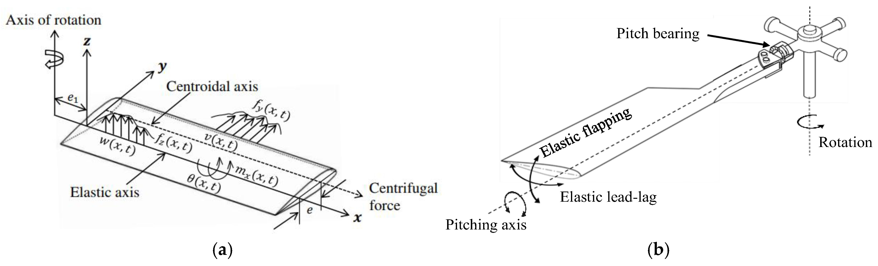
Figure 2.
Typical cross-section of the Bo 105 helicopter rotor blade.
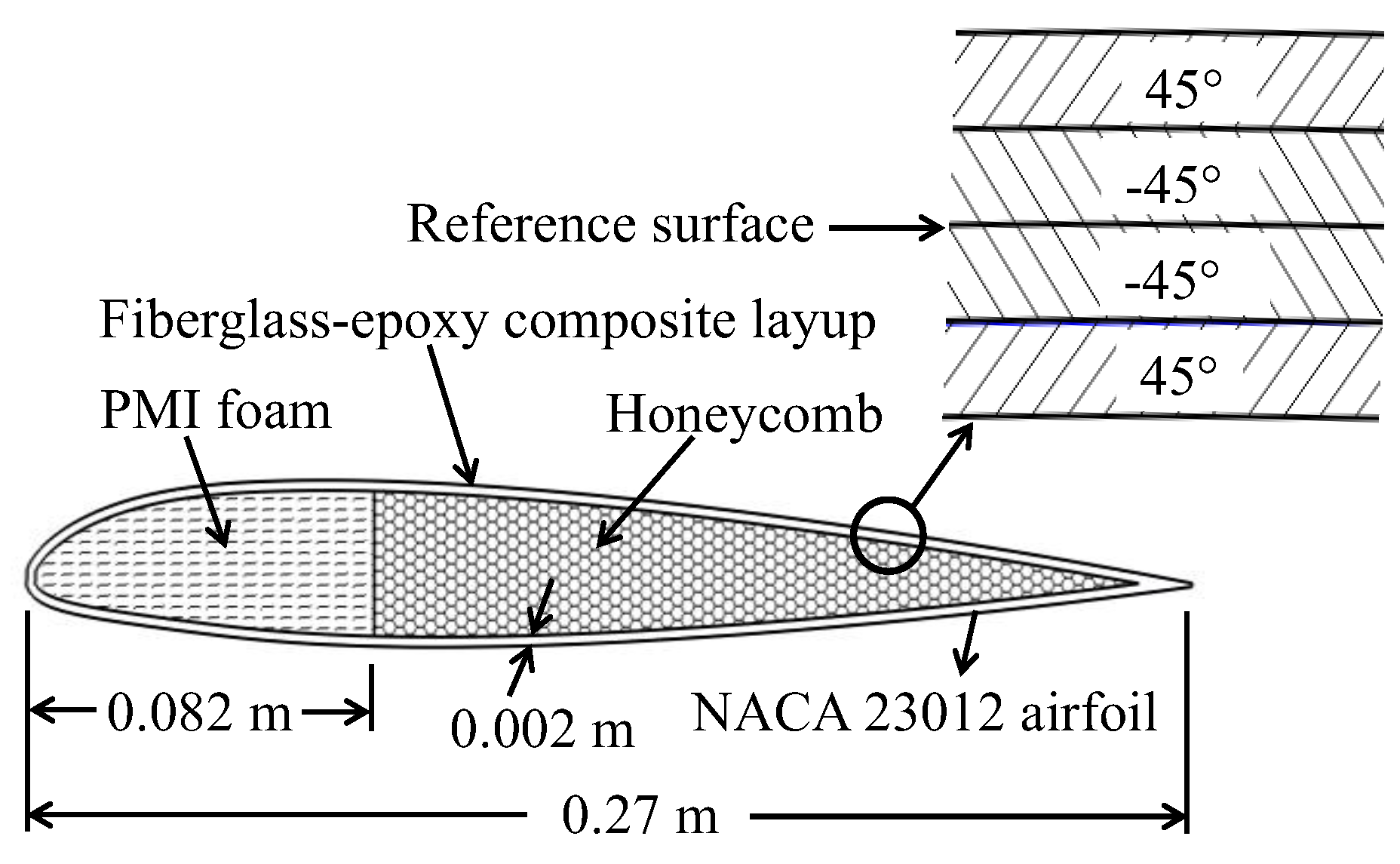
Figure 3.
Generation of the reference surface from the outermost surface of the composite shell, where and are known coordinates of the points on the outermost surface and and are unknown coordinates of the points on the reference surface.
Figure 3.
Generation of the reference surface from the outermost surface of the composite shell, where and are known coordinates of the points on the outermost surface and and are unknown coordinates of the points on the reference surface.
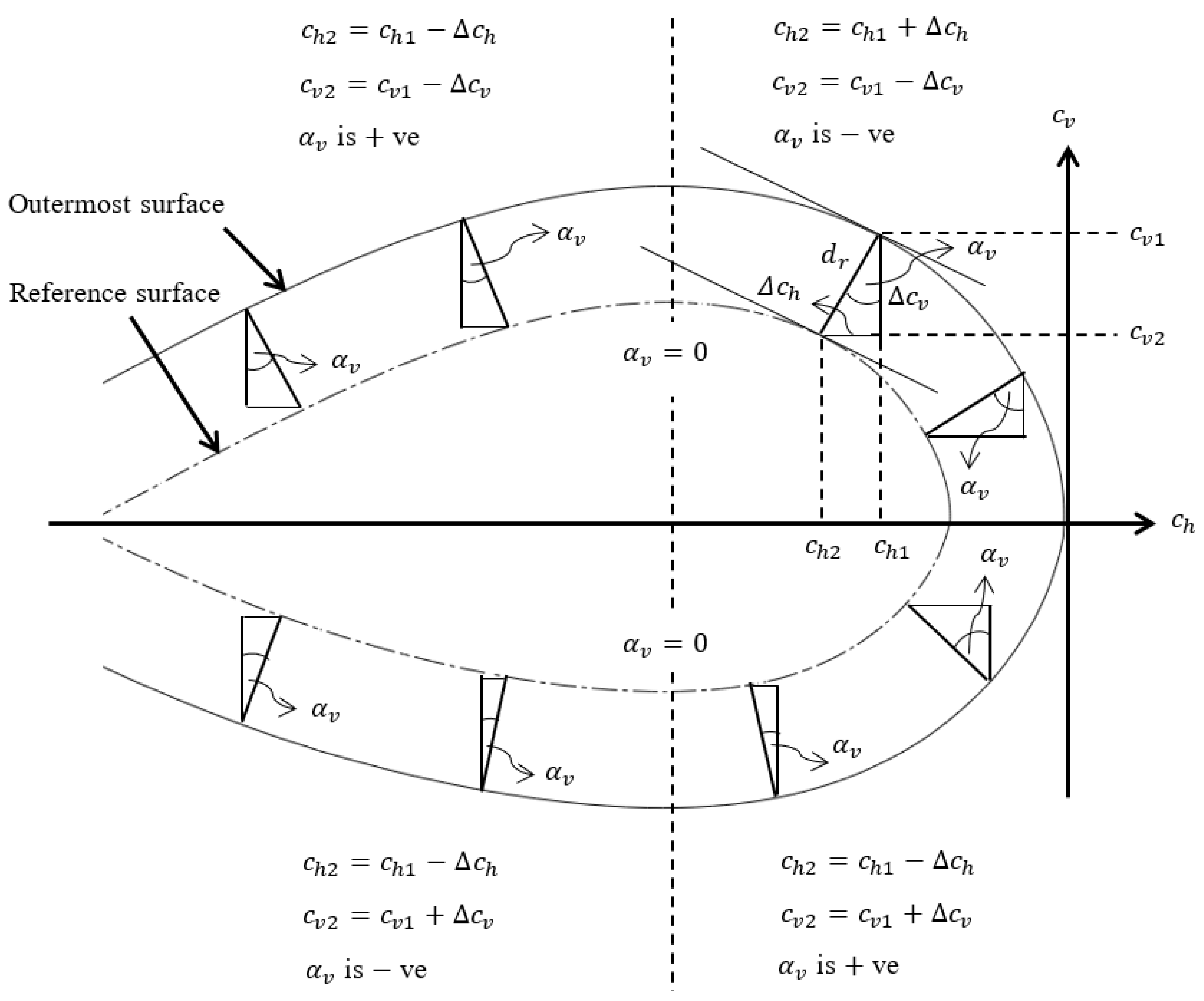
Figure 4.
Various types of sections of thin composite structures: (a) Rectangular; (b) Elliptic; (c) Laminate; (d) Circular; (e) Arbitrary.
Figure 4.
Various types of sections of thin composite structures: (a) Rectangular; (b) Elliptic; (c) Laminate; (d) Circular; (e) Arbitrary.
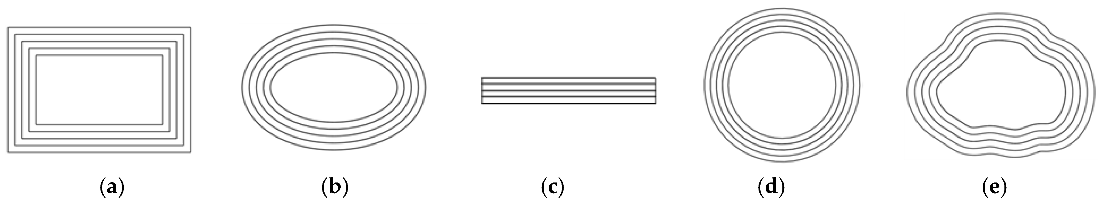
Figure 5.
Location of the centroidal and neutral axis of the cross section.
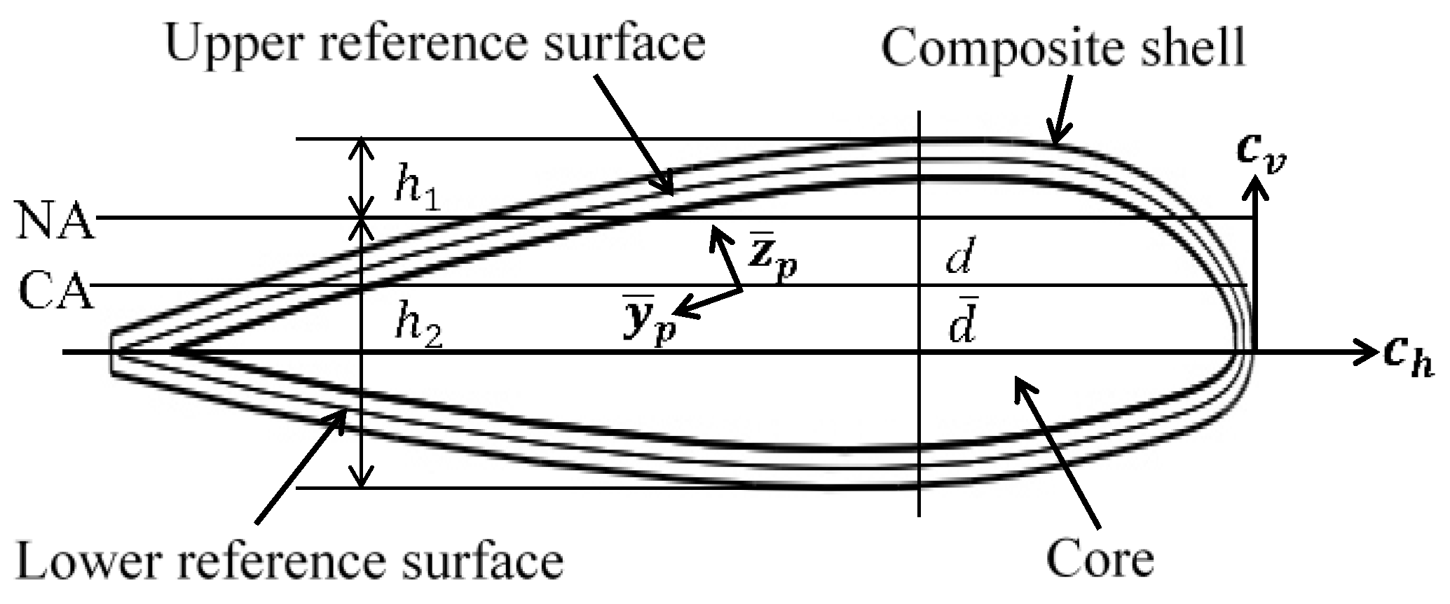
Figure 6.
(a) Finite element domain of the helicopter rotor blade; (b) Magnified view of the converged mesh.
Figure 6.
(a) Finite element domain of the helicopter rotor blade; (b) Magnified view of the converged mesh.
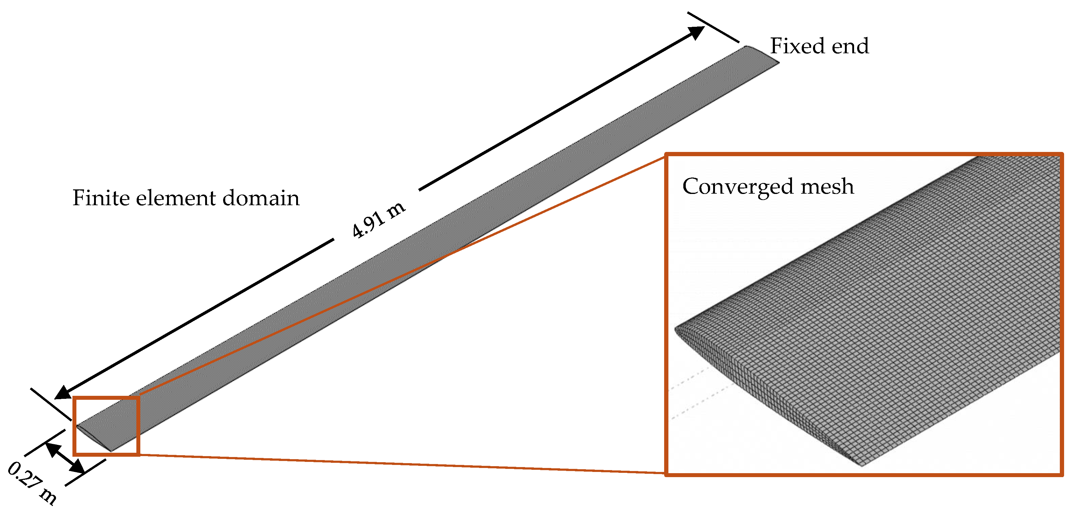
Figure 7.
Schematic of an LQR controller.
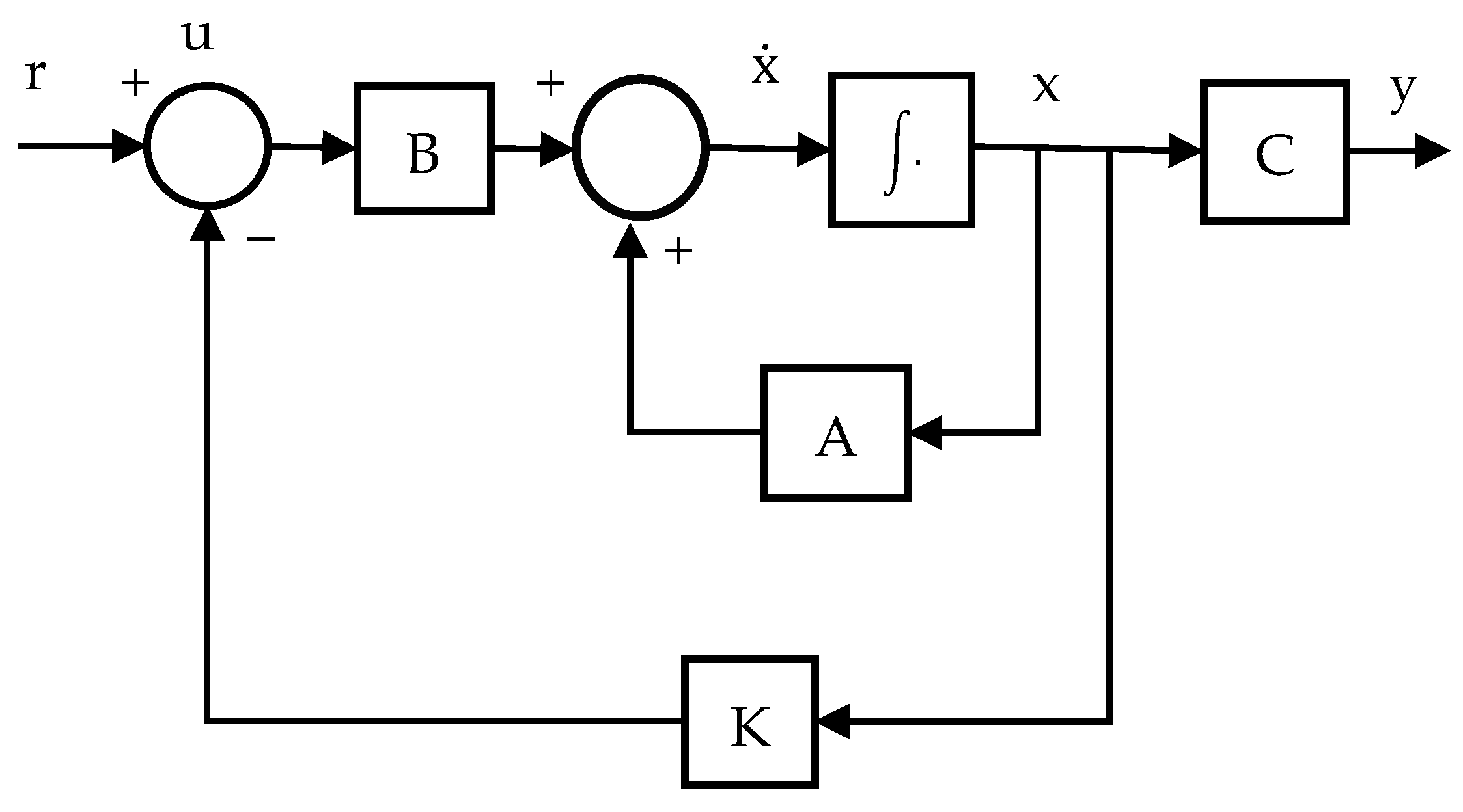
Figure 8.
Variation of the fundamental natural frequencies of the triply coupled vibration of the rotor blade with number of degrees-of-freedom for (a) nonrotating case; (b) rotating case.
Figure 8.
Variation of the fundamental natural frequencies of the triply coupled vibration of the rotor blade with number of degrees-of-freedom for (a) nonrotating case; (b) rotating case.
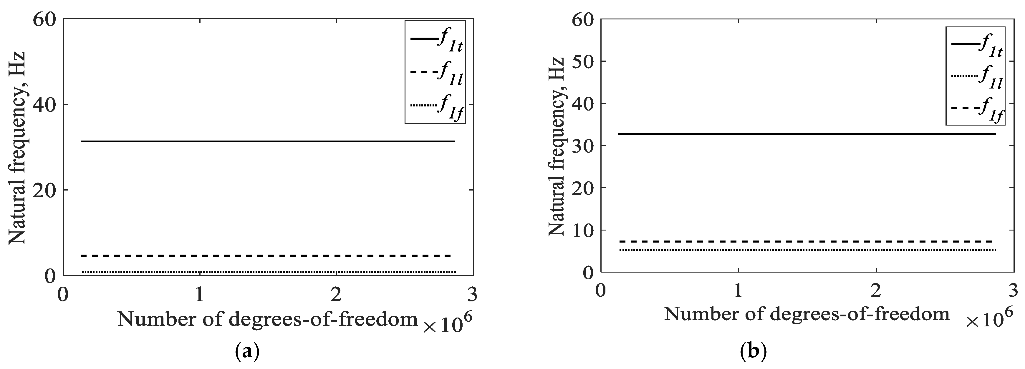
Figure 9.
Mode shapes of the nonrotating blade governed by (a) 1st mode flapping; (b) 1st mode lead-lag; (c) 1st mode torsion; (d) 2nd mode flapping; (e) 2nd mode lead-lag; (f) 2nd mode torsion; (g) 3rd mode flapping; (h) 3rd mode lead-lag; (i) 3rd mode torsion.
Figure 9.
Mode shapes of the nonrotating blade governed by (a) 1st mode flapping; (b) 1st mode lead-lag; (c) 1st mode torsion; (d) 2nd mode flapping; (e) 2nd mode lead-lag; (f) 2nd mode torsion; (g) 3rd mode flapping; (h) 3rd mode lead-lag; (i) 3rd mode torsion.
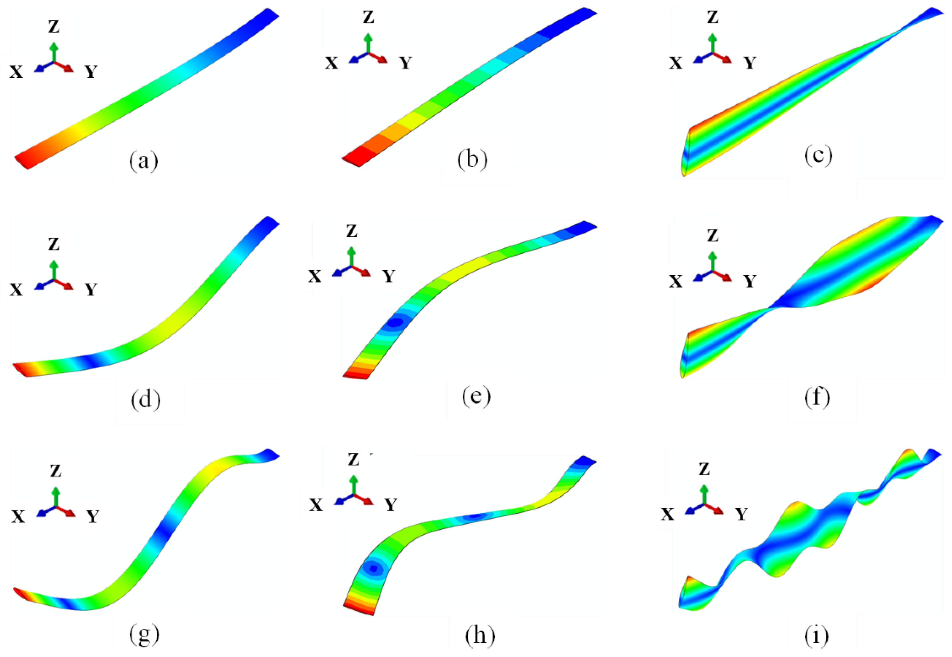
Figure 10.
Mode shapes of the rotating blade governed by (a) 1st mode flapping; (b) 1st mode lead-lag; (c) 1st mode torsion; (d) 2nd mode flapping; (e) 2nd mode lead-lag; (f) 2nd mode torsion; (g) 3rd mode flapping; (h) 3rd mode lead-lag; (i) 3rd mode torsion.
Figure 10.
Mode shapes of the rotating blade governed by (a) 1st mode flapping; (b) 1st mode lead-lag; (c) 1st mode torsion; (d) 2nd mode flapping; (e) 2nd mode lead-lag; (f) 2nd mode torsion; (g) 3rd mode flapping; (h) 3rd mode lead-lag; (i) 3rd mode torsion.
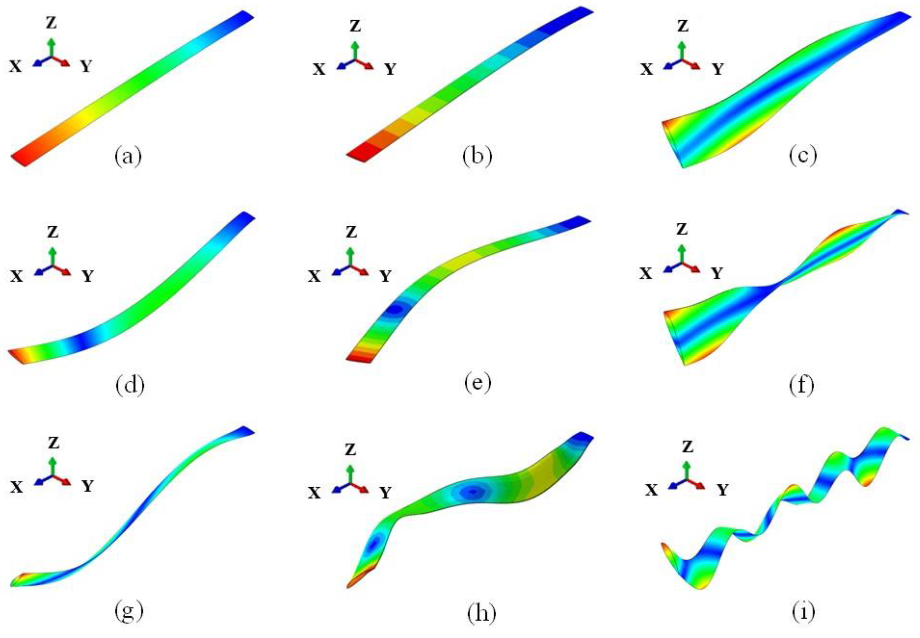
Figure 11.
Controlled flapping tip deflection for 800.
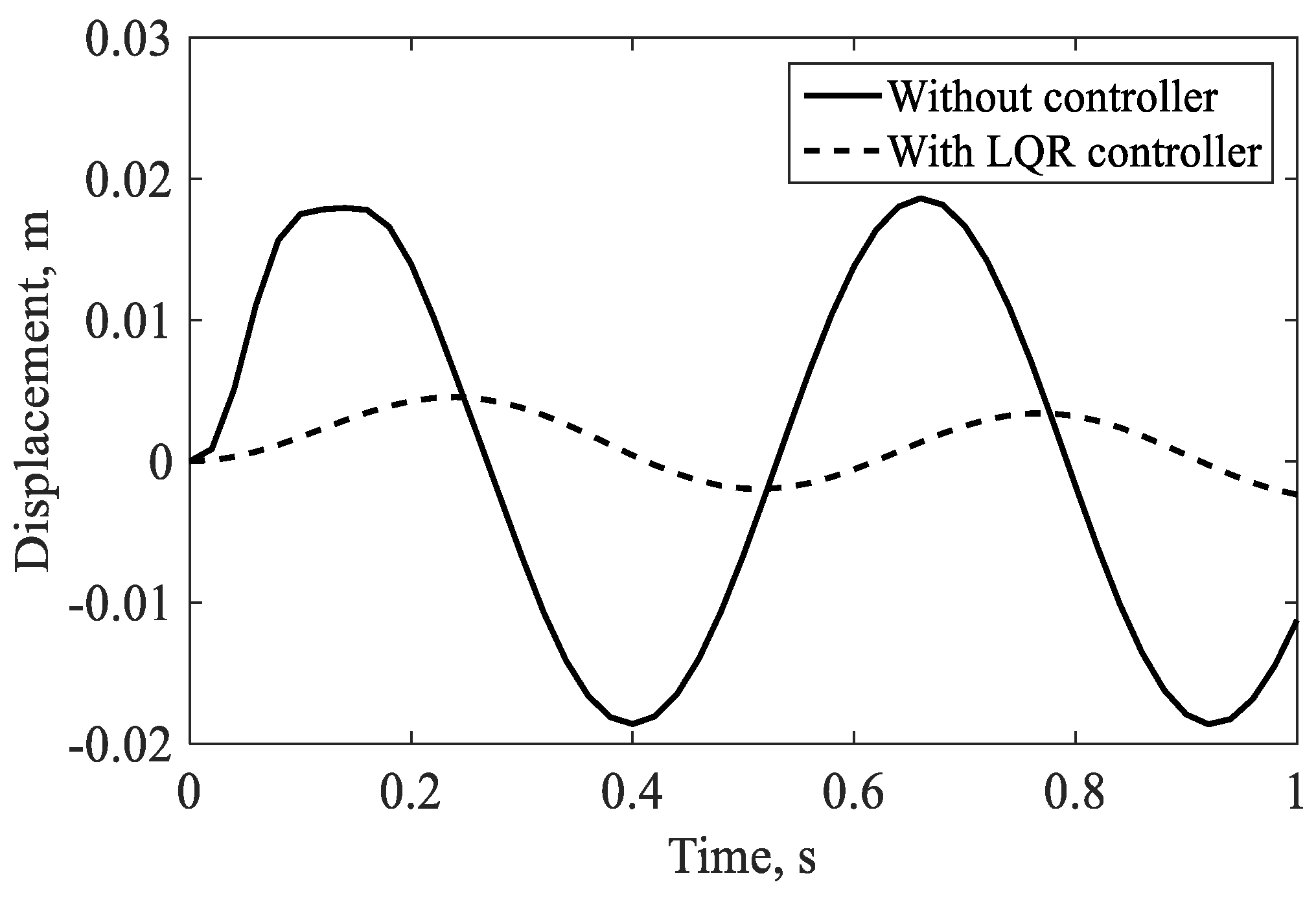
Figure 12.
Controlled lead-lag tip deflection for 2000.
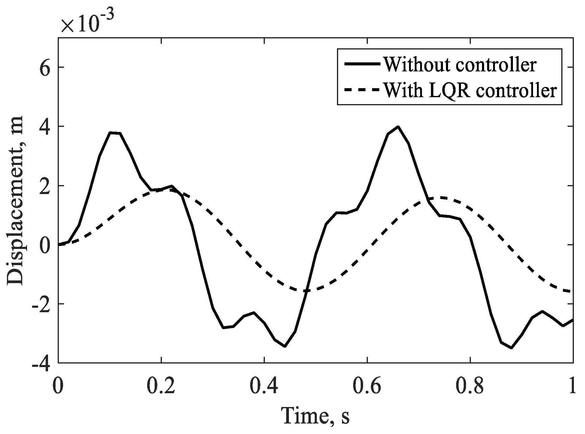
Figure 13.
Controlled torsional tip deflection for 30000.
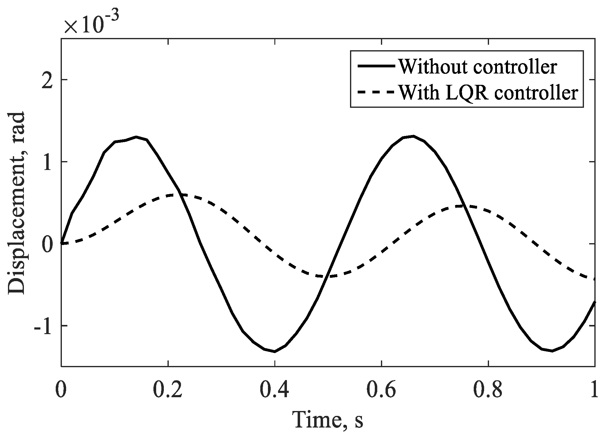
Figure 14.
Controlled flapping tip deflection for 8.
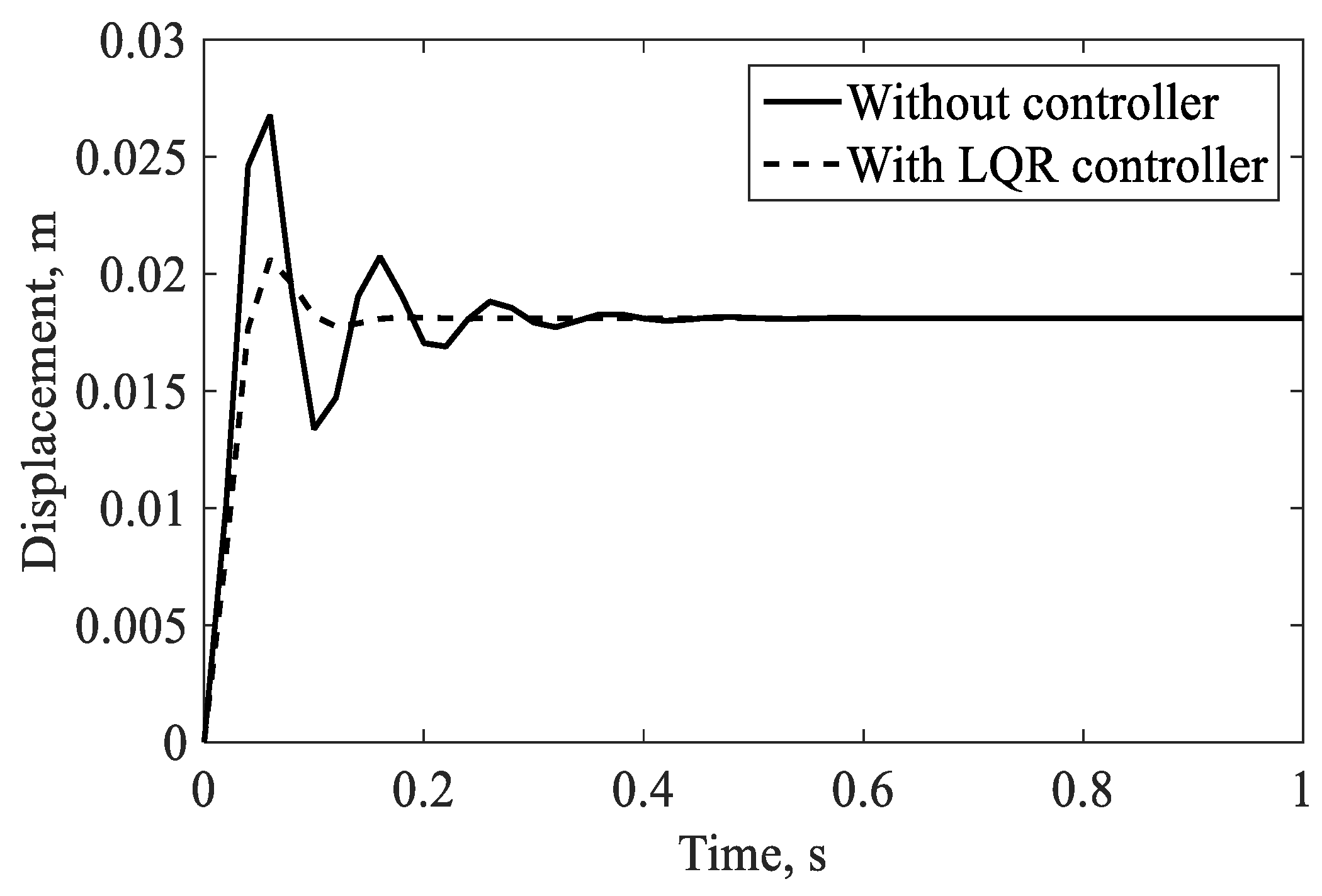
Figure 15.
Controlled lead-lag tip deflection for 16.
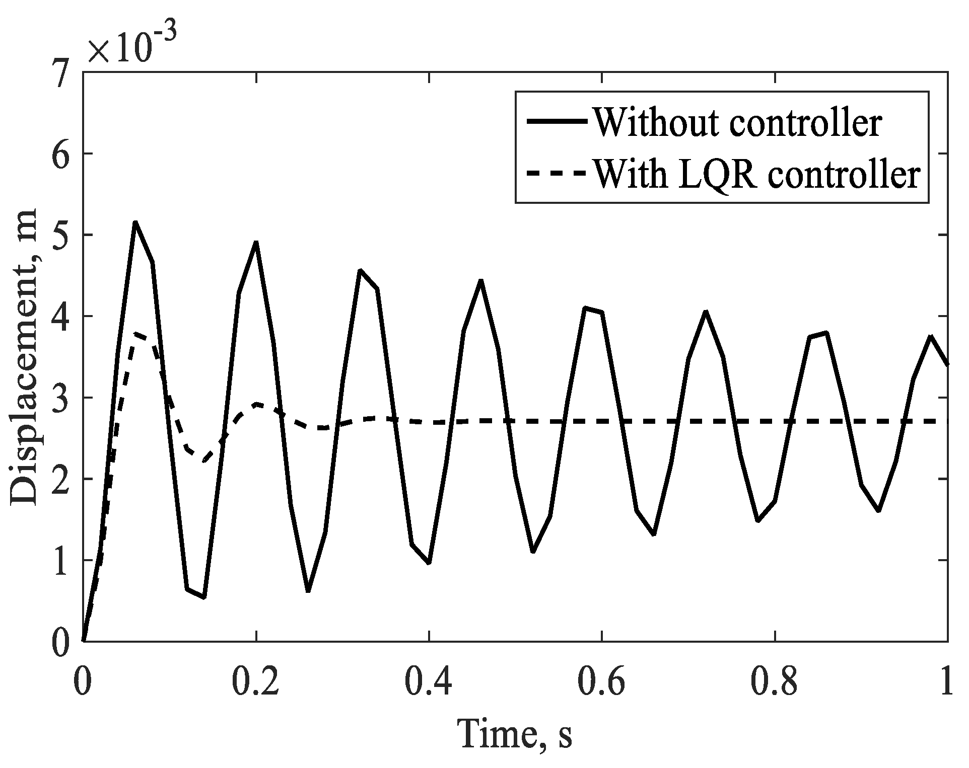
Figure 16.
Controlled torsional tip deflection for 12.
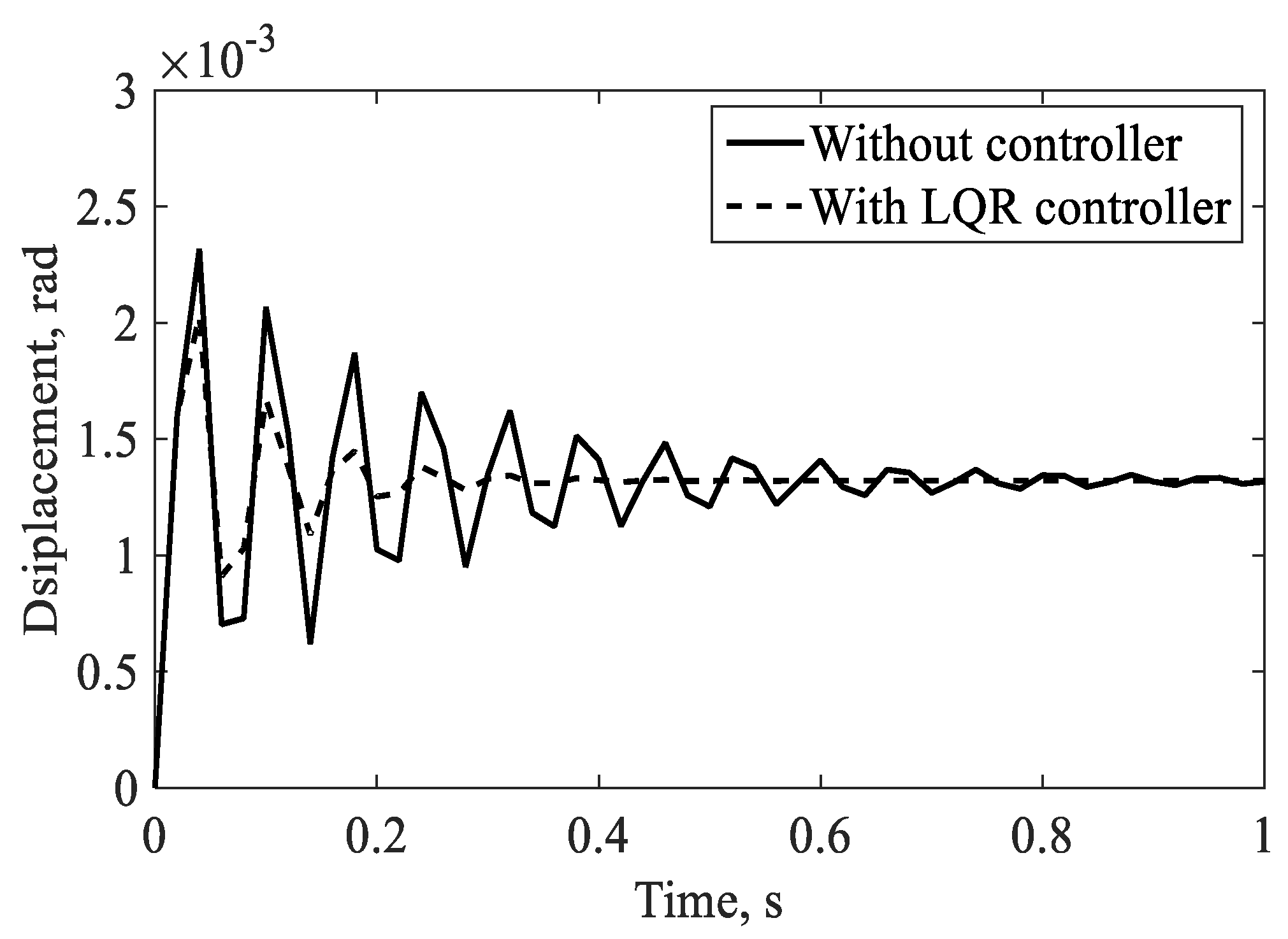
Figure 17.
Controlled flapping tip deflection for 100.
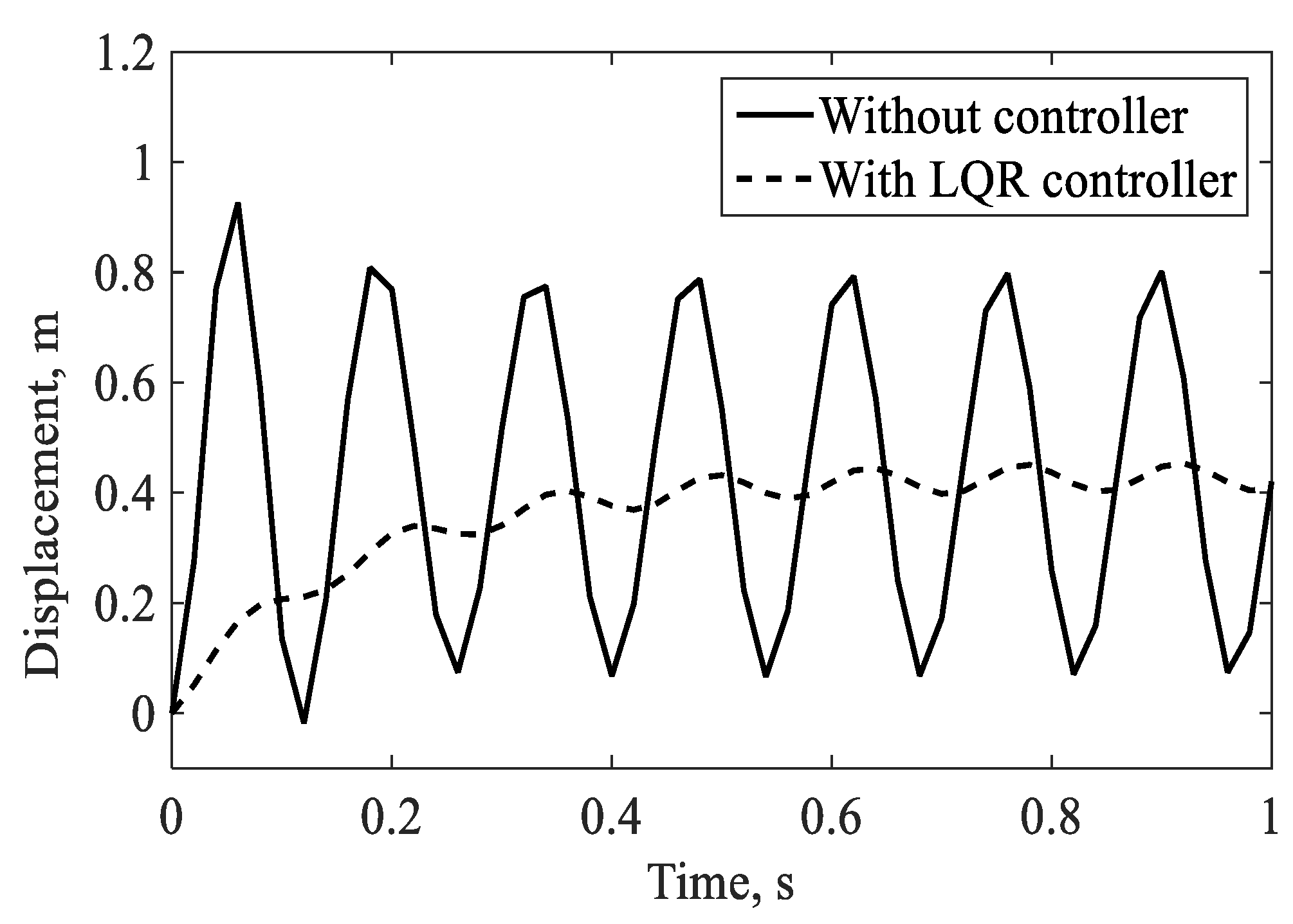
Figure 18.
Controlled lead-lag tip deflection for 500.
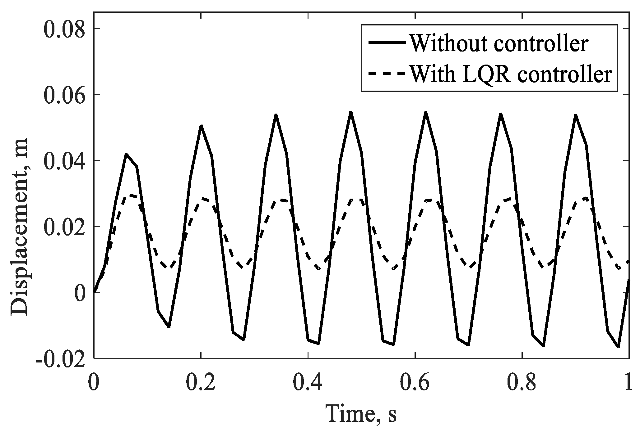
Figure 19.
Controlled torsional tip deflection for 2000.
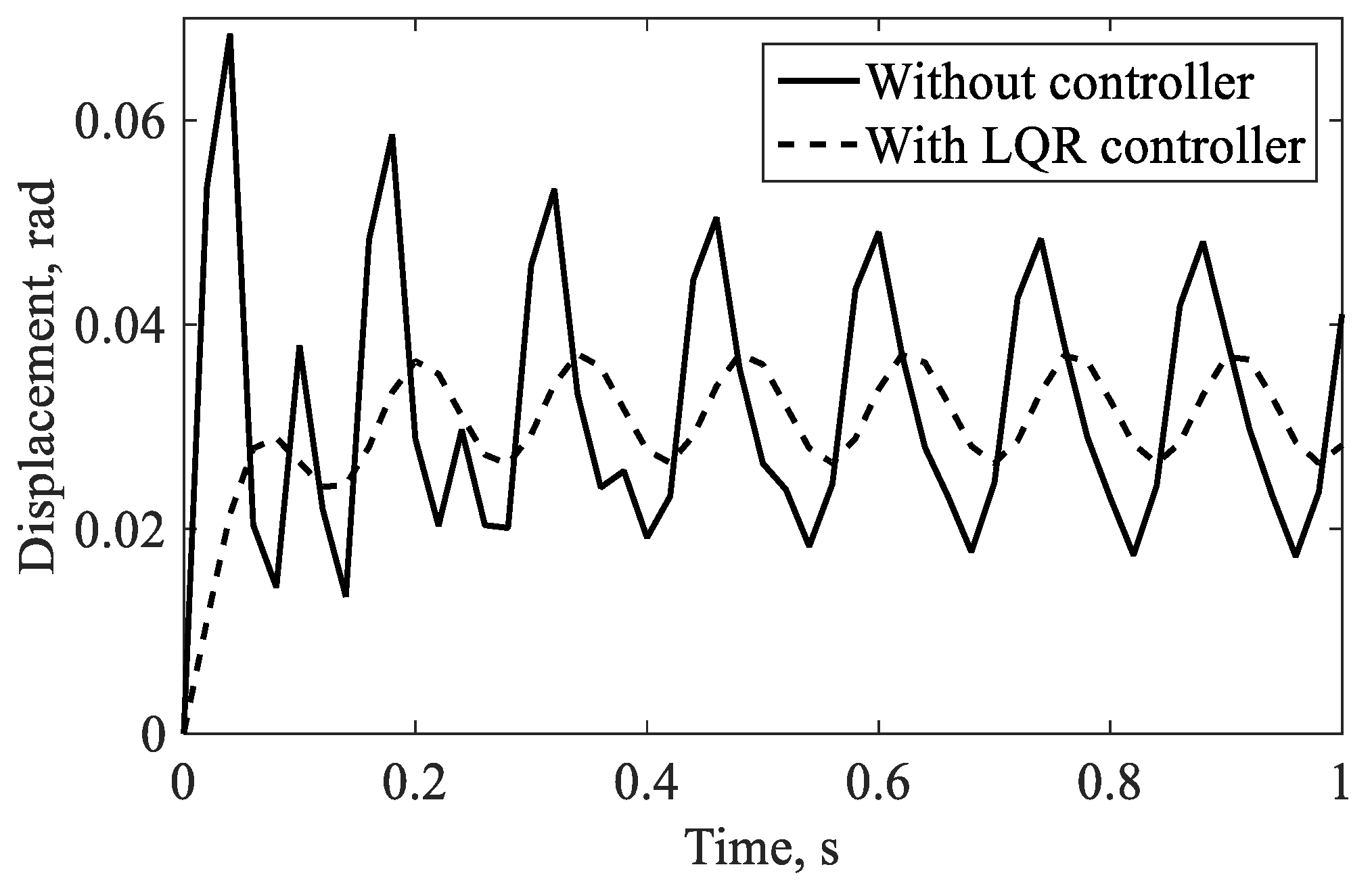
Figure 20.
Controlled flapping tip deflection for 0.002.
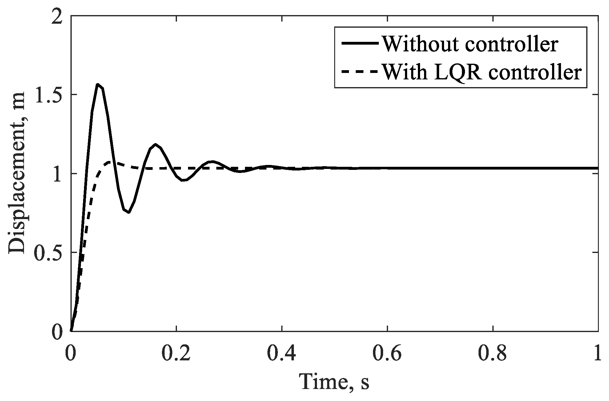
Figure 21.
Controlled lead-lag tip deflection for 0.6.
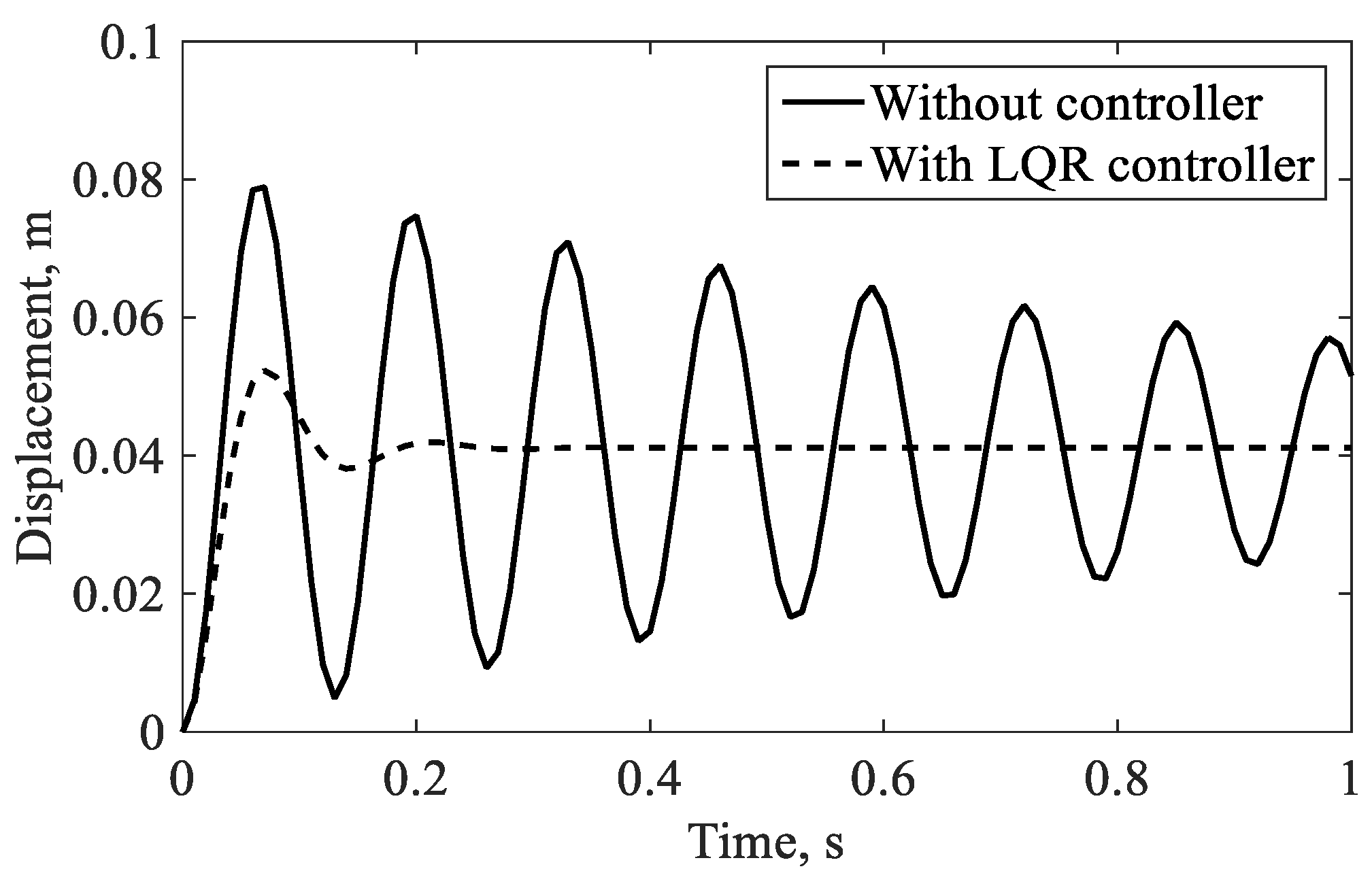
Figure 22.
Controlled torsional tip deflection for 0.006.
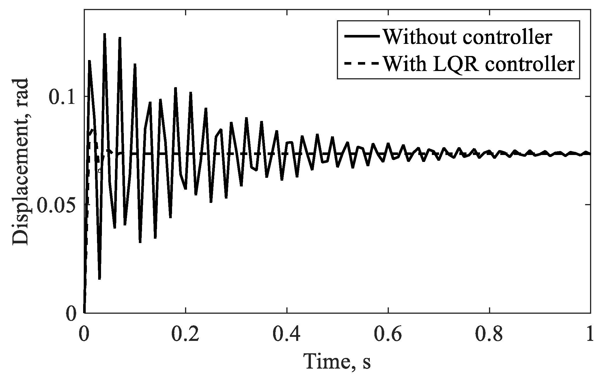
Figure 23.
Variation of normalized vibration amplitudes with the logarithmic scaling of the LQR weighting parameter .
Figure 23.
Variation of normalized vibration amplitudes with the logarithmic scaling of the LQR weighting parameter .
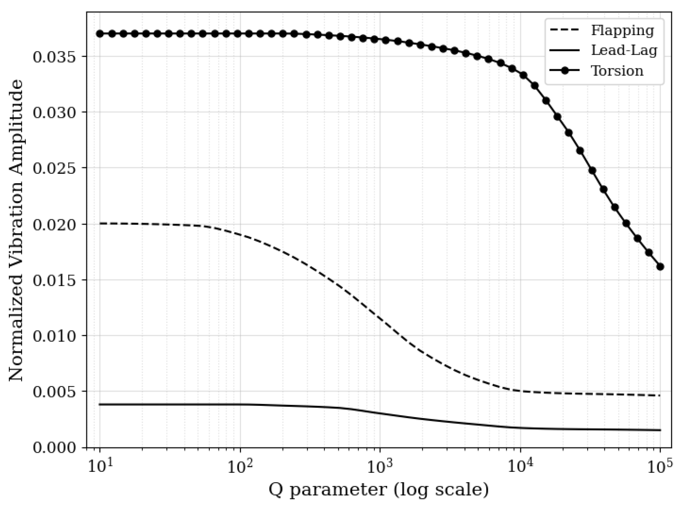

Table 1.
Properties of the outer shell of the composite rotor blade section [25].
Table 1.
Properties of the outer shell of the composite rotor blade section [25].
| Properties | Value | Properties | Value |
|---|---|---|---|
| 2100 kg/m3 | 0.28 | ||
| 45 GPa | 5.5 GPa | ||
| 12 GPa | 0.002 m |
Table 2.
Properties of the Rohacell-Honeycomb isotropic inner core in the composite blade section [25].
Table 2.
Properties of the Rohacell-Honeycomb isotropic inner core in the composite blade section [25].
| Rohacell | Honeycomb | ||
|---|---|---|---|
| Properties | Value | Properties | Value |
| 75 kg/m3 | 48 kg/m3 | ||
| 105 MPa | 128 MPa | ||
Table 3.
Main parameters of the Bo 105 rotor blade [24].
Table 3.
Main parameters of the Bo 105 rotor blade [24].
| Parameters | Value | Parameters | Value |
|---|---|---|---|
| Blade length | 4.61 m | Rotor speed | 44.5 rad/s |
| Chord length | 0.27 m | Blade root offset | 0.30 m |
| Rotor disk area | 75.73 m2 | Number of blades | 4 |
| Blade tip speed | 218.50 m/s | Airfoil | NACA 23012 |
Table 4.
Comparison of natural frequencies of coupled vibration of the rotating blade obtained from the MGM [23] and from experimental research [16].
| Fundamental Natural Frequencies, Hz | |||
|---|---|---|---|
| This study (MGM) | Experimental study | % Error | |
| 7.76 | 7.93 | 2.19 | |
| 5.65 | 5.18 | 8.31 | |
| 29.37 | 25.22 | 14.13 | |
Table 5.
Comparison of vibration attenuation results with the benchmark results [38].
Table 5.
Comparison of vibration attenuation results with the benchmark results [38].
| Mode | This Study (Hovering, Periodic Excitation) | Camino and Santos [38] (Periodic LQR, Full-State Feedback) | Difference |
|---|---|---|---|
| Flapping | 0.020 m−0.0046 m (77% reduction) | Primary bending mode: 70–80% reduction | Within same range |
| Lead–Lag | 0.0038 m−0.0016 m (58% reduction) | Secondary bending mode: 50–65% reduction | Similar range |
| Torsion | 0.037 rad−0.012 rad (68% reduction) | Not reported | Not applicable |
| Trend with | Higher → greater attenuation, higher control effort | Higher → greater attenuation, higher actuator demand | Identical qualitative behavior |
Table 6.
Natural frequencies of the coupled vibration for the nonrotating blade obtained from the MGM [23] and FEA.
Table 6.
Natural frequencies of the coupled vibration for the nonrotating blade obtained from the MGM [23] and FEA.
| Natural Frequencies, Hz | ||||||
|---|---|---|---|---|---|---|
| Mode | This study (MGM) | FEA | This study (MGM) | FEA | This study (MGM) | FEA |
| = 1 | 0.69 | 0.65 | 4.74 | 4.61 | 29.37 | 31.36 |
| = 2 | 4.33 | 4.04 | 29.72 | 28.73 | 88.03 | 93.93 |
| = 3 | 12.13 | 11.27 | 83.22 | 79.48 | 146.60 | 157.10 |
Table 7.
% Error between the frequencies for the nonrotating blade obtained from the MGM [23] and FEA.
Table 7.
% Error between the frequencies for the nonrotating blade obtained from the MGM [23] and FEA.
| % Error | |||
|---|---|---|---|
| Mode | |||
| = 1 | 5.79 | 2.74 | 6.77 |
| = 2 | 6.69 | 3.33 | 6.47 |
| = 3 | 7.08 | 4.49 | 7.16 |
Table 8.
Natural frequencies of the coupled vibration for the rotating blade obtained from the MGM [23] and FEA.
Table 8.
Natural frequencies of the coupled vibration for the rotating blade obtained from the MGM [23] and FEA.
| Natural Frequencies, Hz | ||||||
|---|---|---|---|---|---|---|
| Mode | This study (MGM) | FEA | This study (MGM) | FEA | This study (MGM) | FEA |
| = 1 | 7.76 | 7.27 | 5.65 | 5.42 | 29.37 | 32.88 |
| = 2 | 18.53 | 18.06 | 34.05 | 32.95 | 88.03 | 95.45 |
| = 3 | 32.29 | 30.17 | 88.16 | 83.96 | 146.62 | 161.02 |
Table 9.
% Error between the frequencies for the rotating blade obtained from the MGM [23] and FEA.
Table 9.
% Error between the frequencies for the rotating blade obtained from the MGM [23] and FEA.
| % Error | |||
|---|---|---|---|
| = 1 | 6.32 | 4.07 | 10.67 |
| = 2 | 2.54 | 3.23 | 7.77 |
| = 3 | 6.57 | 4.76 | 8.94 |
Disclaimer/Publisher’s Note: The statements, opinions and data contained in all publications are solely those of the individual author(s) and contributor(s) and not of MDPI and/or the editor(s). MDPI and/or the editor(s) disclaim responsibility for any injury to people or property resulting from any ideas, methods, instructions or products referred to in the content. |
© 2025 by the authors. Licensee MDPI, Basel, Switzerland. This article is an open access article distributed under the terms and conditions of the Creative Commons Attribution (CC BY) license (http://creativecommons.org/licenses/by/4.0/).
Copyright: This open access article is published under a Creative Commons CC BY 4.0 license, which permit the free download, distribution, and reuse, provided that the author and preprint are cited in any reuse.


