
Submitted:
01 December 2025
Posted:
02 December 2025
You are already at the latest version
Abstract
For nearly eighty years after the discovery of the electron's anomalous magnetic moment researchers have relied on extremely laborious quantum methods for the calculation of an elementary particle anomalous g-factor. Since the derivation of single exact method for the calculation of such a fundamental parameter have been considered inconceivable the quantum theory of vacuum have been established as unique tool to that goal. Based on thorough theoretical research about the origin of elementary particles' anomalous magnetic moment the present paper reveals a scalar field approach describing the named anomaly as non-quantum phenomena and underlying the exact calculation of the charged leptons anomalous g-factor and self-interaction energy. Impressive accuracy in reproducing the most recent experimental data for the electron's and muon's anomalous g-factor is demonstrated. Exact calculation of the spin angular momentum dynamics and atomic energy spectrum in terms of specific invariant mass contributing to the anomalous magnetic moment is also reported. Apparent particle-antiparticle asymmetry is obtained. The presented approach integrates fundamental aspects from electrodynamics and scalar field theory and shed light on an experimentally tested aspect of a theoretical framework independent on the quantum vacuum theory, with completely removed divergences and closely intertwined with the Standard Model predictions.
Keywords:
anomalous magnetic moment
; electrodynamics
; scalar field theory
; electron
; muon
1. Introduction
The anomalous g-factor is a characteristic quantifying the influence of the vacuum on elementary particles’ intrinsic magnetic moment. It is one of the essential fundamental physical parameters for putting our current understanding about the particles inherent environment to the test. Being able to theoretically reproduce the experimentally measured value of an anomalous g-factor with unprecedented accuracy is accepted as indisputable prove to the validity of the theoretical methods in use. Therefore, the attempts to rationalize methods and theories beyond the Standard Model (SM) over the gap between measured and calculated value of the muon anomalous g-factor have risen to unprecedentedly high levels over the last two decades [1,2,3,4,5,6,7,8,9,10,11,12,13,14,15,16]. The discovery of the electron’s anomalous magnetic moment [17,18,19,20,21], nowadays detected with stunning precision [22,23], has established the believe that the occurrence of such anomaly is merely quantum effect and uniquely addressable only by the quantum theory. The quantum vacuum picture [24,25,26,27,28,29,30,31,32,33] theorized along the successful calculation of the electron’s anomalous g-factor after decades of research [33,34,35,36,37] and constantly studied in attempt to provide results for the muon’s anomalous g-factor with high accuracy [30,38,39,40,41,42,43,44,45,46] is accepted as a sole approach to the description of bare particles inherent environment. Seemingly justifying all inevitable renormalization procedures – as pointed out by one of the developers of quantum electrodynamics (see Ref. [47,48]), the impressively accurate quantum computations devised to calculate the electron’s and muon’s magnetic moment anomalies seems to have implied almost no reservations when it comes to the uniqueness of quantum vacuum approach. Nevertheless, on the background of such laborious approach and the constant search for a new physics beyond SM [49,50,51] the absence of a comprehensible formulation of such a fundamental physical quantity can not help but raise questions concerning the existence of a single exact analytical approach to its calculation. The present absence of theoretical framework underpinning such calculations and all attempts to its derivation within the theory of relativity and quantum theory left no room for confusion. A general exact calculation of leptons anomalous g-factor [52,53] and the contribution of corresponding self-interaction into the particle’s action is neither underlined by the classical nor quantum gauge field. Remarkably, all efforts indicate that a primary physical model underlying such results would require only stationary vacuum and non-symmetry based field terms of the Lagrangian.
Addressing the challenge of formulating the action quantifying exactly the contribution of such fundamental parameter into the particle’s worldline, the current study presents a profound view on the origin of anomalous magnetic moment. It reveals that independently on the quantum theory of the vacuum and its contribution to observables there exist an exact self-consistent approach to the calculation of self-interaction energy and anomalous g-factor of a massive non-composite particle having elementary electric charge. The theoretical framework underlying the named approach utilizes the point-particle model as a description of the particle’s dynamics and field theory to describe the particle’s inherent environment and account for the dynamics of its spin angular momentum. The study demonstrates that in contrast to the quantum vacuum approach the calculation of anomalous g-factor and self-interaction energy can be brought about by considering the particle’s inherent environment as composed of four real spin-zero stationary fields that are only electromagnetic in nature. All four fields are given as explicit functions obtained as solution to the corresponding Euler-Lagrange equations. Essentially, with respect to these solutions the reported approach distinguish two cases. One describing unstable non-composite particles and the other a stable one. For an unstable particle two of all four real scalar fields are massless and the anomalous g-factor appears as solution to the following transcendental equation
where
is the fine structure constant, m is the particle’s rest mass and is the total rest mass of the particle’s decay product. It is further demonstrated that for a stable particle the number of massless scalar fields increases to three, with vanishing . In this case a unique transcendental equation with no free mass parameters is derived, reading
The study unequivocally points out that the used mathematical framework admits only one stable massive electrically charged elementary particle with anomalous g-factor calculated via Equation (2). In addition to the main results related to Equations (1) and (2) the paper reports equations of motion describing the particle’s spin angular momentum dynamics and discuss the principal interrelationship with quantum theory.
The rest of the paper is organized as follows. Section 2 presents the initial assumptions the devised exact approach is based on and depicts its most recent results. Section 3 revises and discusses in details the mathematical framework used to devise the exact approach to the calculation of considered particle’s anomalous g-factor and corresponding self-interaction energy. It provides a thorough representation and interpretation of all relevant physical quantities and equations. In Section 4 we demonstrate that the atomic energy spectrum can be calculated in terms of specific invariant mass contributing to the magnitude of anomalous magnetic moment. Section 5 provides concluding remarks and summarizes the theory’s main aspects. All computations and 3D illustrations are carried out on Wolfram Mathematica. The plots are generated by gnuplot.
2. Principle Formulations and Calculations
2.1. Principal and General Relations
Equations (1) and (2) are derived by taking into account two principal considerations. First, it is assumed that as a result of the interplay with its inherent environment the considered particle may be viewed as gaining additional rest energy and equivalently a rest mass. The gained rest mass contributes to the particle’s gyromagnetic ratio by a fraction exactly equal to the corresponding anomalous g-factor. Accordingly, the anomalous g-factor is considered as a ratio between the particle’s self-interaction energy and rest energy. The higher the self-interaction energy the greater the corresponding anomalous g-factor and vice versa. This principal formulation reads
where c is the light speed in vacuum and is the particle’s self-interaction energy. Second, the self-interaction energy is defined as the total energy of the particle’s interaction with its intrinsic environment assumed to be only electromagnetic in nature. It is calculated exactly as the average interaction over the characteristic spherically symmetric spatial domain , with radial boundary , where is the reduced Compton wavelength associated to the particle. We have
where is the volume of , q is the electric charge associated to the particle and represents a superposition of four real spin-zero fields describing the particle’s inherent environment. Given with respect to the particle’s rest frame of reference, we have the singularity free radial function
where is the electric constant, r is the radial distance from the origin of particle’s rest frame of reference and is a scaling parameter. In particular,
Graphical representation is depicted in Figure 1.
2.2. Comparison with the Experimental Data
Recently it was reported that the calculation of muon’s anomalous g-factor via Equation (7), or equivalently Equation (1), leads to a difference of about 60 ppt (see Ref. [53]) with respect to the world average reported in Ref. [46] uncovering more accurate theoretical result than the one obtained after quantum vacuum approach [43]. With respect to the most recent average value fixed after the third FNAL measurement [55] the difference increases to 184 ppt, see Figure 2 and Table 1. The most probable decay product of the muon was taken into account, with , where is the electron’s rest mass and kg is the sum of muon neutrino and anti-electron neutrino rest masses. Accordingly, it is suggested that the upper bound on the sum of muon neutrino and anti-electron neutrino rest masses is equal to , with corresponding rest energy of about eV. This result is consistent with the reported upper bound on the total rest energy of the three flavor neutrino eV [56] and far below the bound on effective anti-electron neutrino rest energy obtained from the most recent KATRIN data analysis [57]. Essentially, Equation (1) yields exact value for the muon anomalous g-factor that surpasses by accuracy the most recent quantum field theory prediction [54], see Figure 2 and Table 1. The value of electron and muon rest masses is taken from NIST [58] yielding , where is the muon’s rest mass. The value of fine structure constant is fixed with respect to the solution of Equation (2).
Remarkably, for the integral in Equation (7) yields Equation (2) with solution representing a highly accurate result for the electron’s anomalous g-factor, where the one reported in Ref. [52] agrees with the most recent experimental value [23] (see Figure 3) to ppt, with calculated fine structure constant . Comparison with the single electron cyclotron measurement data [22] and the most recent agreement on the values obtained from quantum field theory calculations [37,59] is further depicted in Figure 3.
Within the considered approach the particle’s anomalous magnetic moment appears to be entirely of electromagnetic origin and the vacuum is described by a superposition of four stationary non-interacting real scalar fields. Such a rationalization differs from the established in the quantum theory vacuum picture in terms of which depending on the bare particle’s mass different vacuum contributions adds up to correct the corresponding g-factor [33,37,41,43,60,61,62].
Shedding light on an unrevealed avenue to the calculations of the muon’s anomalous g-factor the presented results unequivocally points out to the lack of discrepancy between theory and experiment. The used approach suggests that the anomalous magnetic moment is not explicitly quantum by nature and has solely electromagnetic origin proposing an entirely different picture about the particles inherent electromagnetic field, resulting self-interaction and the vacuum. Moreover, it makes a direct reference to the stability of the electron by predicting its anomalous g-factor in the absence of any free parameter that may characterize the electron, see Equation (2).
3. Theoretical Framework
3.1. The Action
To gain further insight on the approach underlying Equation (7) with all resulting data and conclusions, let us focus on the total energy of the considered system and study the action describing it.
Consider the system composed of spin-half particle with rest mass m, electric charge q and intrinsic magnetic moment as isolated, where is the corresponding g-factor, is the corresponding magneton and is the particle’s spin angular momentum. Obtaining the results in Equations (1) and (2) requires to set the mathematical framework in terms of the following considerations. The particle’s dynamics in spacetime is described with the aid of the point-particle model. The particle’s spin angular momentum is precessing about the axis of relative motion, with oscillation energy equal to the particle’s relativistic energy and corresponding rest energy representing a fraction of the particle’s rest energy. The particle does not propagate in effective electromagnetic field inherent to it. The electromagnetic field associated to the particle is not characterized by intensity. It is characterized by potentials that are uniquely defined as the average of a superposition of non-interacting massless and massive centrally symmetric real spin-zero fields describing the particle’s inherent environment. The superposition of these field’s is time independent, divergence free, it vanish for and at large distances from the particle.
Within the given framework, the action of the considered system is represented as a sum of four terms. The first term quantify the contribution of particle’s rest energy into its worldline. The second one has no contribution and is related to the dynamics of particle’s spin angular momentum. The third and forth ones account for the contribution of self-interaction energy and that of the particle’s intrinsic environment, respectively. In particular, we have
where is the particle’s four-momentum, , with is a vector function determining the dynamics of particle’s spin angular momentum, is the four-momentum associated that dynamics, is the four-current density, is the electromagnetic field four-potential, is a normalization coefficient, is a real spin-zero field, with scaling parameter for . Generally, there are two massless and two massive spin-zero fields. Here, the enumeration of these fields is such that for the two massless ones, we have . Moreover, is the proper time and standard summation convention is used for all indices.
Essentially, we have the explicit representations and relations
, where is the particle’s relative velocity, is the corresponding Lorentz factor, ℏ is the reduced Plank constant, is the wave vector characterizing the dynamics of the particle’s spin, is the corresponding frequency, is the particle’s charge density in its rest frame of reference with origin , is the electromagnetic field scalar potential associated with the particle and is the wave number characterizing the spin dynamics in the absence of relative motion. In the particle’s rest frame of reference the oscillation frequency is and we have , where is the transverse wave vector component, with magnitude . Furthermore, we have the continuity equation and the condition . The latter condition points out that the electromagnetic field inherent to the particle is not characterized by intensity. Therefore, there is a gauge freedom , but the Lorenz condition is trivially satisfied, with for all , where are the corresponding electromagnetic field tensor components and is an arbitrary scalar function. In the considered system, the electromagnetic field do not contribute to the system’s stress-energy tensor. Only in the presence of additional electrically charged particle the corresponding electromagnetic field will be characterized by intensity. In the general case of a multiparticle system the total electromagnetic field four-potential will be a sum of two terms. One uniquely defined with respect to the underlying real scalar fields and the particles’ characteristic spatial domains and the other depending explicitly on time and independent on the particles’ dynamics. As a result, the equations of corresponding electrodynamics will include the homogeneous Maxwell’s equations and those satisfied by the scalar fields inherent to each particle, with no necessity of solutions describing advanced and retarded electromagnetic field potentials [63,64,65,66]. At large distances the scalar potentials will resemble the Coulomb one only that the inhomogeneous electromagnetic field equations will be redundant.
Representing the Lagrangian from Equation (8) in terms of the particle’s rest mass and the stationary spin-zero fields, we have
where we take into account the relation , with being an infinitesimal time interval in the observational frame of reference. Here, indicates that the spatial integral runs over the entire three-dimensional space. The second term on the right hand side vanish and has no contribution to the Lagrangian and corresponding Hamiltonian. It equals zero, since it does not quantify the particle’s dynamics but that of its spin angular momentum. It response to variation. Since the dynamics of considered system is completely determined the components of are represented neither as field density nor as a series expansion over the particle’s momentum space.
3.2. The Hamiltonian
Since the scalar fields describing the particle’s intrinsic environment do not propagate independently from it, the system’s generalized momentum is related only to the particle’s relative motion. The system’s Hamiltonian reads
Here, for convenience the Lagrangian is written as
where
are the particle’s self-interaction energy (see Equations (3) and (4)) and the effective rest mass quantifying the contribution of the particle’s inherent environment into the system’s total rest energy, respectively. Accordingly, taking into account Equation (3), from Equations (10) and (11) we obtain the Hamiltonian
where is the particle’s effective rest mass and . The vacuum energy is represented by the term , with effective rest mass distributed in space in accordance to Equation (12), where the coefficients ensure the integral is finite. In the case of an antiparticle, , showing that as an isolated system an antiparticle will be energetically disadvantageous than its matter counterpart for which . Therefore, the energy gap between a system composed of particle and that composed of its antiparticle is , such that in the case of particle the Hamiltonian in Equation (13) reduces to . In the absence of electric charge the scalar fields vanish and the Hamiltonian in Equation (13) represents only the relativistic energy with no energy gap underlying the discussed particle-antiparticle asymmetry.
3.3. Field Equations
The explicit representation of vector function and the calculation of self-interaction energy along with the effective mass term given in Equation (12) follows the solution of Euler-Lagrange equations derived from the variation of action given in Equation (8). We have two independent groups of equations. The first group represents the equations of motion
with the Lorenz condition . Respecting all imposed constraints, the solutions of Equation (14) are obtained as a superposition of two polarization states,
where for all , we have the constraints and , are the polarization vectors satisfying and . The star symbol indicates complex conjugate and we further have
Both polarization vectors satisfy the condition appearing analogous to the Lorenz condition.
The second group is a system of homogeneous screened Poison equations satisfied by the given real spin-zero fields,
with the parametric and boundary conditions
For all , the given conditions reduce the system of equations (16) into two Laplace and two homogeneous screened Poison equations, with solutions
where , and , , respectively. The representation of both non-zero scaling parameters follows the principal formulation given in Equation (3) yielding the superposition in Equation (5), with and . The particle’s charge appears as a particular upper bond on the superposition of all scalar fields and reads
Expressed in position space the superposition in Equation (5) may be viewed as a generalized Coulomb potential with regularized singularity at . The regularization terms are parametrized by unique to the particle bounds on the corresponding momentum space representing the scaling parameters and . In other words, we have the Fourier transform
with two regulators [53,67,68,69] enclosed in the rectangular brackets and leading to the Yukawa potentials and .
3.4. The Particle’s Spin
Geometrically, the solutions given in Equation (15) represent two orthogonal unit vectors rotating about the axis of particle’s propagation and underlie the dynamics of transverse spin angular momentum components. Accordingly, the particle’s spin angular momentum is precessing about the origin of particle’s rest frame of reference, with symmetry axis coinciding with that of the particle’s relative motion and with energy distinct from the relativistic energy. The angle of rotation of transverse spin components is , where is the corresponding four-position vector. In the case of right circular polarization (see Figure 4) the helicity is positive and vice versa. Therefore, the spin angular momentum can be expressed as a linear combination of solutions given in Equation (15) and their cross product. We have
where s is the corresponding spin quantum number. With selected as the symmetry axis, or , from Equation (17) one gets
where and . Here the plus and minus signs stand for positive and negative helicity, respectively. Furthermore, the plus-minus sign subscript label on the vector is omitted for the sake of clarity. Within the presented framework and considered system the spin angular momentum is a constant of motion and hence represents the considered system’s total angular momentum. The result given in Equation (17) is related only to the case of spin-half and spin-one non-composite particles, where giving the functions in Equation (15) particular amplitude and considering a collection of such particles, we can transit to quantum theory by applying the occupation number scheme. Let us point out that from Equation (14) and all given constraints follows the equation . Therefore, by applying the substitutions and , we can reimpose the intrinsic quantities such as the field vector, tangential and angular velocities presented in Refs. [52,53].
The oscillation energy underlies the spin angular momentum dynamics and is necessary for the derivation of Equations (1) and (2). Its introduction allows to distinct the representation of four-momentum and when transitioning to quantum theory. As the particle is propagating with four-momentum and its spin angular momentum is precessing about the axis of propagation with four-momentum , the system under consideration may apparently demonstrate simultaneously point-like and wave-like behavior. Since the ratio between the invariants and is constant equal to and neither the spinor fields nor wave functions that may approximately describe the considered system within quantum theory are observables, with a convenient normalization the four-momentum operator can be quantitatively associated to both and . However, since the particle’s four-momentum accounts for only the relative motion of its rest frame of reference with known position vector, the qualitative approach would require to set , with energy and momentum uncertainties related to the system’s oscillation dynamics and not its relative motion. The particle’s orbital angular momentum related to its relative motion, like in a cyclotron, will have continuous eigenspectrum. On contrary, the orbital angular momentum associated to the system’s oscillation dynamics may be characterized by a discrete eigenspectrum, like in atoms. Therefore, while preserving the principles of relativity the oscillation energy can be quantized allowing to reproduce the energy spectrum of a quantum system without losing locality. Moreover, the invariants and can be related to different metric in . In case the particle has no electric charge, like a neutrino, the invariant vanish and as a propagating wave the neutrino will appear massless even if it is characterized by rest mass.
3.5. Multi-Particle System
Consider a system composed of multiple unbound particles each described by the action given in Equation (8) when considered as isolated. The particles interact electromagnetically with interaction underlined by the superposition of all real scalar fields associated to the particles. The equations of motion of an arbitrary particle in the system can be derived from the corresponding action. The latter reads
where standard summation convention is used for all repeating indices, the i-th particle characteristics and associated quantities discussed in details in terms of Equation (8) are labeled by the corresponding subscript, on the understanding that . The last term on the right hand side in Equation (19) accounts for the electromagnetic field’s energy, with corresponding tensor components . The electromagnetic field is locally emergent and does not occur in the space between the particles and independently of their configuration in space. Accordingly, the four-potential do not depend explicitly on time and is not an independent variable in the corresponding Lagrangian density, only the real scalar field are. For all , the number of scalar fields equals the number of particles. Here, we take into account that the i-th particle’s space-time interval reads . Moreover, we have
where n runs over the number of all particles and for all i the electromagnetic field scalar potential depends on the coordinates of all particles. The equations of motion describing the i-th particle dynamics follow from the variation of first and third terms on the right hand side in Equation (19) with respect to the particle’s position in space-time. For all i the variation of second and fourth terms leads to Equations (14) and (16), respectively. From the variation of fifth term follows the homogeneous Maxwell equations which are trivially satisfied since the four-potential does not depend explicitly on time.
In particular, accounting for the relations and , from the variation of first and third terms in the action (19), we obtain the equations of motion
where is the i-th particle proper time. The spatial component of the four-force given in Equation (20) is the Lorentz force known from electrodynamics [65]. In particular, for , we have , where and are the electric and magnetic intensities, respectively, of the electromagnetic field at the origin of i-th particle rest frame of reference. Moreover, taking into account the relation from the variation of the fifth term we get the covariant form of corresponding homogeneous Maxwell equations, .
Let us point out that electrodynamics suggesting a description of the considered system on a macroscopic level results as an approximation to the presented theory. The approximation requires removal of the second and forth terms in the action (19) and transitioning to effective macroscopic electromagnetic field with a single four-potential and tensor. Such a transition, however, will reimpose the use of renormalization procedures once the quantum counterpart of the field is considered.
4. Atomic Energy Spectrum
The energy underlying the particle’s spin angular momentum dynamics and representing the temporal component of four-momentum is dependent on the particle’s relative motion but the corresponding rest energy is invariant. Within such consideration, it is expected that under the action of external fields the particle gains additional oscillation energy related to the occurrence of orbital angular momentum and corresponding to more complex dynamics. Thus, depending on the type of interaction the resulting oscillation dynamics may be characterized by discrete energy spectrum. Prominent examples of such systems are atoms with atomic shells representing different mode of oscillation. The corresponding oscillation energy is quantized with respect to the invariant .
Within the framework of all previous considerations and by analogy to Equation (14) the atomic energy levels and corresponding orbital angular momentum are obtained after considering the Klein-Gordon equation
where , and is the effective electromagnetic field four-potential associated to the nucleus. The vector functions and differ by a complex amplitude describing the atom’s spatial properties, with . As a result, Equation (21) reduces to a system of two equations. One describing the dynamics of transverse spin angular momentum components (see Equation (14)) in the absence of relative motion and a Helmholtz equation satisfied by the given amplitude yielding the atomic energy level sequence in the absence of fine and hyperfine structures. We have
where we take into account that , ,
Here, E is the total energy of the oscillator, with potential energy selected to be of Coulomb type and similarly to the condition after Equation (18), we have the constraint that fix the spin angular momentum transverse components with respect to the radial unit vector . Let us note that Equation (21) reduces to Equation (14) at the limit for which and .
For the second equation in (22) reduces to the Schrodinger equation describing non-relativistic atomic energy spectrum (see also Ref. [52]) with solutions being orthogonal polynomials , where are the radial wave functions, are the spherical harmonics, , and are the main, orbital and magnetic orbital quantum numbers, respectively. For more details on the atomic energy spectrum in the absence of fine and hyperfine structures the reader may consult Refs. [70,71,72]. The obtained solutions yield the non-relativistic energy spectrum for . Reproducing the energy spectrum at relativistic limit is feasible for .
5. Summary
The devised mathematical framework with action given in Equation (8) abides by the principles of theory of relativity and presents a completely different picture about the electromagnetic vacuum and particle’s self-interaction from that established in the quantum theory. It yields non-Maxwell divergence free field equations (see Equation (16)) and set of transcendental equations (see Equations (1) and (2)) allowing researchers to calculate the anomalous g-factor of the charged leptons with remarkable accuracy, see Figs. 2 and 3. Equations of motion (see Equation (14)) describing exactly the particle’s spin angular momentum dynamics are also derived shedding light on the apparent wave-like behavior associated with the particle. The reported results show that a vacuum composed of four stationary real scalar fields can provide a complete description of the elementary particles self-interaction and anomalous magnetic moment. What is intriguing is that the field part of the action in Equation (8) appears to have no underlying symmetry. It is either not symmetric by origin or a broken underlying symmetry is not apparent within the given representation. Looking forward, the identification of such a symmetry along with the mechanism breaking it would be a significant step in uncovering more about what may lies beyond SM. Certainly, with no embedded gauge symmetry the corresponding Lagrangian (see Equation (9)) cannot be canonically related to the one in quantum electrodynamics. In deriving Equations (1) and (2) neither the particle’s inherent electromagnetic field is time and spatially dependent gauge field nor a spinor field is required to map the considered particle’s dynamics and that of its spin. The electromagnetic field potentials are uniquely defined and no coupling between the underlying real scalar fields and a spinor or other fictitious field is required. The presented theory is singularity free and the energy scale is fixed with respect to the particle’s invariant mass. Accordingly, no renormalization procedure follows, notions like bare mass, pole mass and running parameters have no basis.
Author Contributions
Not applicable.
Funding
Not applicable.
Institutional Review Board Statement
Not applicable.
Informed Consent Statement
Not applicable.
Data Availability Statement
In addition to the provided supplementary information, all data supporting the current study are available within the article and from the corresponding authors on reasonable request.
Acknowledgments
The author thanks Nikolay M. Nikolov and Hamed Pejhan for the useful comments and fruitful discussion on the presented approach and results.
Conflicts of Interest
Not applicable.
References
- Pires, C.A.D.S.; Rodrigues Da Silva, P.S. Scalar scenarios contributing to (g-2)μ with enhanced Yukawa couplings. Phys. Rev. D 2001, 64, 117701. [Google Scholar] [CrossRef]
- Arroyo-Ureña, M.A.; Hernández-Tomé, G.; Tavares-Velasco, G. Anomalous magnetic and weak magnetic dipole moments of the τ lepton in the simplest little Higgs model. Eur. Phys. J. C 2017, 77, 227. [Google Scholar] [CrossRef]
- De Conto, G.; Pleitez, V. Electron and muon anomalous magnetic dipole moment in a 3-3-1 model. J. High Energ. Phys. 2017, 2017, 104. [Google Scholar] [CrossRef]
- Majumdar, C.; Patra, S.; Pritimita, P.; Senapati, S.; Yajnik, U.A. Neutrino mass, mixing and muon g-2 explanation in U(1)Lμ-Lτ extension of left-right theory. J. High Energ. Phys. 2020, 2020, 10. [Google Scholar] [CrossRef]
- Calibbi, L.; López-Ibáñez, M.L.; Melis, A.; Vives, O. Muon and electron g-2 and lepton masses in flavor models. J. High Energ. Phys. 2020, 2020, 87. [Google Scholar] [CrossRef]
- Leutgeb, J.; Mager, J.; Rebhan, A. Holographic QCD and the muon anomalous magnetic moment. Eur. Phys. J. C 2021, 81, 1008. [Google Scholar] [CrossRef]
- Díaz Sáez, B.; Ghorbani, K. Singlet scalars as dark matter and the muon (g-2) anomaly. Phys. Lett. B 2021, 823, 136750. [Google Scholar] [CrossRef]
- Cadeddu, M.; Cargioli, N.; Dordei, F.; Giunti, C.; Picciau, E. Muon and electron g-2 and proton and cesium weak charges implications on dark Zd models. Phys. Rev. D 2021, 104, L011701. [Google Scholar] [CrossRef]
- Hong, T.T.; Nha, N.H.T.; Nguyen, T.P.; Phuong, L.T.T.; Hue, L.T. Decays h→eaeb, eb→eaγ, and (g-2)e,μ in a 3-3-1 model with inverse seesaw neutrinos. PTEP 2022, 2022, 093B05. [Google Scholar] [CrossRef]
- Raya, K.; Bashir, A.; Miramontes, A.S.; Roig, P. Dyson-Schwinger equations and the muon g-2. Supl. Rev. Mex. Fis. 2022, 3, 020709. [Google Scholar] [CrossRef]
- Takeuchi, M.; Iguro, S.; Kitahara, T.; Lang, M.S. Current status of the muon g-2 interpretations within two-Higgs-doublet models. Phys. Rev. D 2023, 108, 115012. [Google Scholar] [CrossRef]
- Dinh, D. Muon anomalous magnetic dipole moment in a low scale type I see-saw model. Nucl. Phys. B 2023, 994, 116306. [Google Scholar] [CrossRef]
- Cao, J.; Meng, L.; Yue, Y. Electron and muon anomalous magnetic moments in the Z3-NMSSM. Phys. Rev. D 2023, 108, 035043. [Google Scholar] [CrossRef]
- Li, H.; Wang, P. Nonlocal QED and lepton g-2 anomalies. Eur. Phys. J. C 2024, 84, 654. [Google Scholar] [CrossRef]
- Huang, D.; Geng, C.Q.; Wu, J. Unitarity bounds on the massive spin-2 particle explanation of muon g-2 anomaly. Eur. Phys. J. C 2024, 84, 246. [Google Scholar] [CrossRef]
- Erdelyi, B.A.; Gröber, R.; Selimovic, N. Probing New Physics with the Electron Yukawa coupling. arXiv 2025. [Google Scholar] [CrossRef]
- Breit, G. Does the Electron Have an Intrinsic Magnetic Moment? Phys. Rev. 1947, 72, 984–984. [Google Scholar] [CrossRef]
- Kusch, P.; Foley, H.M. The Magnetic Moment of the Electron. Phys. Rev. 1948, 74, 250–263. [Google Scholar] [CrossRef]
- Schwinger, J. On Quantum-Electrodynamics and the Magnetic Moment of the Electron. Phys. Rev. 1948, 73, 416–417. [Google Scholar] [CrossRef]
- Kusch, P. The Magnetic Moment of the Electron. Nobel Lecture 1995. [Google Scholar]
- Roberts, B.L.; Marciano, W.J. Lepton Dipole Moments; Vol. 20, Advanced Series on Directions in High Energy Physics, World Scientific, 2009. [CrossRef]
- Hanneke, D.; Fogwell, S.; Gabrielse, G. New Measurement of the Electron Magnetic Moment and the Fine Structure Constant. Phys. Rev. Lett. 2008, 100. [Google Scholar] [CrossRef]
- Fan, X.; Myers, T.; Sukra, B.; Gabrielse, G. Measurement of the Electron Magnetic Moment. Phys. Rev. Lett. 2023, 130, 071801. [Google Scholar] [CrossRef]
- Schwinger, J. Quantum Electrodynamics. II. Vacuum Polarization and Self-Energy. Phys. Rev. 1949, 75, 651–679. [Google Scholar] [CrossRef]
- Karplus, R.; Kroll, N.M. Fourth-Order Corrections in Quantum Electrodynamics and the Magnetic Moment of the Electron. Phys. Rev. 1950, 77, 536–549. [Google Scholar] [CrossRef]
- Kataev, A.L. Analytical eighth-order light-by-light QED contributions from leptons with heavier masses to the anomalous magnetic moment of electron. Phys. Rev. D 2012, 86, 013010. [Google Scholar] [CrossRef]
- King, B.; Heinzl, T. Measuring vacuum polarization with high-power lasers. HPLSE 2016, 4, e5. [Google Scholar] [CrossRef]
- Morte, M.D.; Francis, A.; Gülpers, V.; Herdoíza, G.; Von Hippel, G.; Horch, H.; Jäger, B.; Meyer, H.B.; Nyffeler, A.; Wittig, H. The hadronic vacuum polarization contribution to the muon g-2 from lattice QCD. J. High Energ. Phys. 2017, 2017, 20. [Google Scholar] [CrossRef]
- Westin, A.; Kamleh, W.; Young, R.; Zanotti, J.; Horsley, R.; Nakamura, Y.; Perlt, H.; Rakow, P.; Schierholz, G.; Stüben, H. Anomalous magnetic moment of the muon with dynamical QCD+QED. EPJ Web Conf. 2020, 245, 06035. [Google Scholar] [CrossRef]
- Gérardin, A. The anomalous magnetic moment of the muon: status of lattice QCD calculations. Eur. Phys. J. A 2021, 57, 116. [Google Scholar] [CrossRef] [PubMed]
- Nedelko, S.; Nikolskii, A.; Voronin, V. Soft gluon fields and anomalous magnetic moment of muon. J. Phys. G: Nucl. Part. Phys. 2022, 49, 035003. [Google Scholar] [CrossRef]
- Melo, D.; Reyes, E.; Fazio, R. Hadronic Light-by-Light Corrections to the Muon Anomalous Magnetic Moment. Particles 2024, 7, 327–381. [Google Scholar] [CrossRef]
- Volkov, S. Calculation of lepton magnetic moments in quantum electrodynamics: A justification of the flexible divergence elimination method. Phys. Rev. D 2024, 109, 036012. [Google Scholar] [CrossRef]
- Laporta, S.; Remiddi, E. Analytic QED Calculations of the Anomalous Magnetic Moment of the Electron. In Advanced Series on Directions in High Energy Physics; World Scientific, 2009; Vol. 20, pp. 119–156. [CrossRef]
- Vogel, M. The anomalous magnetic moment of the electron. Contemp. Phys. 2009, 50, 437–452. [Google Scholar] [CrossRef]
- Aoyama, T.; Hayakawa, M.; Kinoshita, T.; Nio, M. Tenth-order electron anomalous magnetic moment: Contribution of diagrams without closed lepton loops. Phys. Rev. D 2015, 91, 033006. [Google Scholar] [CrossRef]
- Aoyama, T.; Kinoshita, T.; Nio, M. Theory of the Anomalous Magnetic Moment of the Electron. Atoms 2019, 7, 28. [Google Scholar] [CrossRef]
- Farley, F. The 47 years of muon g-2. Prog. Part. Nucl. Phys. 2004, 52, 1–83. [Google Scholar] [CrossRef]
- Miller, J.P.; De Rafael, E.; Lee Roberts, B. Muon (g-2): experiment and theory. Rep. Prog. Phys. 2007, 70, R03. [Google Scholar] [CrossRef] [PubMed]
- Jegerlehner, F.; Nyffeler, A. The muon g-2. Phys. Rep. 2009, 477, 1–110. [Google Scholar] [CrossRef]
- Jegerlehner, F. The Anomalous Magnetic Moment of the Muon; Vol. 274, Springer Tracts in Modern Physics, Springer International Publishing: Cham, 2017. [Google Scholar] [CrossRef]
- Logashenko, I.B.; Eidelman, S.I. Anomalous magnetic moment of the muon. Phys.-Usp. 2018, 61, 480–510. [Google Scholar] [CrossRef]
- Aoyama, T.; Asmussen, N.; Benayoun, M.; Bijnens, J.; Blum, T.; Bruno, M.; Caprini, I.; Carloni Calame, C.; Cé, M.; Colangelo, G.; et al. The anomalous magnetic moment of the muon in the Standard Model. Phys. Rep. 2020, 887, 1–166. [Google Scholar] [CrossRef]
- Keshavarzi, A.; Khaw, K.S.; Yoshioka, T. Muon g-2: A review. Nucl. Phys. B 2022, 975, 115675. [Google Scholar] [CrossRef]
- Aguillard, D.P.; Albahri, T.; Allspach, D.; Anisenkov, A.; Badgley, K.; Baeßler, S.; Bailey, I.; Bailey, L.; Baranov, V.A.; Barlas-Yucel, E.; et al. Measurement of the Positive Muon Anomalous Magnetic Moment to 0.20 ppm. Phys. Rev. Lett. 2023, 131, 161802. [Google Scholar] [CrossRef]
- Aguillard, D.; Albahri, T.; Allspach, D.; Anisenkov, A.; Badgley, K.; Baeßler, S.; Bailey, I.; Bailey, L.; Baranov, V.; Barlas-Yucel, E.; et al. Detailed report on the measurement of the positive muon anomalous magnetic moment to 0.20 ppm. Phys. Rev. D 2024, 110, 032009. [Google Scholar] [CrossRef]
- Dyson, F.J. Divergence of Perturbation Theory in Quantum Electrodynamics. Phys. Rev. 1952, 85, 631–632. [Google Scholar] [CrossRef]
- Todorov, I. From Euler’s play with infinite series to the anomalous magnetic moment. arXiv 2018. [Google Scholar] [CrossRef]
- Borsanyi, S.; Fodor, Z.; Guenther, J.N.; Hoelbling, C.; Katz, S.D.; Lellouch, L.; Lippert, T.; Miura, K.; Parato, L.; Szabo, K.K.; et al. Leading hadronic contribution to the muon magnetic moment from lattice QCD. Nature 2021, 593, 51–55. [Google Scholar] [CrossRef] [PubMed]
- Athron, P.; Fowlie, A.; Lu, C.T.; Wu, L.; Wu, Y.; Zhu, B. Hadronic uncertainties versus new physics for the W boson mass and Muon g-2 anomalies. Nat. Commun. 2023, 14, 659. [Google Scholar] [CrossRef] [PubMed]
- Crivellin, A.; Mellado, B. Anomalies in particle physics and their implications for physics beyond the standard model. Nat. Rev. Phys. 2024, 6, 294–309. [Google Scholar] [CrossRef]
- Georgiev, M. Exact classical approach to the electron’s self-energy and anomalous g-factor. Europhys. Lett. 2024, 147, 20001. [Google Scholar] [CrossRef]
- Georgiev, M. Yukawa Cut-Offs to Model the Muon Self-Interaction. Contemp. Math. 2025, 6, 4762–4775. [Google Scholar] [CrossRef]
- Aliberti, R.; Aoyama, T.; Balzani, E.; Bashir, A.; Benton, G.; Bijnens, J.; Biloshytskyi, V.; Blum, T.; Boito, D.; Bruno, M.; et al. The anomalous magnetic moment of the muon in the Standard Model: an update. Phys. Rep. 2025, 1143, 1–158. [Google Scholar] [CrossRef]
- Aguillard, D.P.; Albahri, T.; Allspach, D.; Annala, J.; Badgley, K.; Baeßler, S.; Bailey, I.; Bailey, L.; Barlas-Yucel, E.; Barrett, T.; et al. Measurement of the Positive Muon Anomalous Magnetic Moment to 127 ppb. Phys. Rev. Lett. 2025, 135, 101802. [Google Scholar] [CrossRef]
- Planck Collaboration. ; Aghanim, N.; Akrami, Y.; Ashdown, M.; Aumont, J.; Baccigalupi, C.; Ballardini, M.; Banday, A.J.; Barreiro, R.B.; Bartolo, N.; et al. Planck 2018 results: VI. Cosmological parameters. A & A 2020, 641, A6. [Google Scholar] [CrossRef]
- KATRIN Collaboration. ; Aker, M.; Batzler, D.; Beglarian, A.; Behrens, J.; Beisenkötter, J.; Biassoni, M.; Bieringer, B.; Biondi, Y.; Block, F.; et al. Direct neutrino-mass measurement based on 259 days of KATRIN data. Science 2025, 388, 180–185. [Google Scholar] [CrossRef] [PubMed]
- 2018 CODATA Value: electron mass and muon mass. The NIST Reference on Constants, Units, and Uncertainty. NIST, 2019.
- Aoyama, T.; Hayakawa, M.; Kinoshita, T.; Nio, M. Tenth-Order QED Contribution to the Electron g-2 and an Improved Value of the Fine Structure Constant. Phys. Rev. Lett. 2012, 109, 111807. [Google Scholar] [CrossRef]
- Labzowsky, L.N.; Goidenko, I. Chapter 8 QED theory of atoms. In Theoretical and Computational Chemistry; Elsevier, 2002; Vol. 11, pp. 401–467. [CrossRef]
- Melnikov, K.; Vainshtein, A. Theory of the Muon Anomalous Magnetic Moment; Vol. 216, Springer Tracts in Modern Physics, Springer Berlin Heidelberg, 2006. [CrossRef]
- Özgüven, Y.; Billur, A.A.; İnan, S.C.; Bahar, M.K.; Köksal, M. Search for the anomalous electromagnetic moments of tau lepton through electron-photon scattering at CLIC. Nucl. Phys. B 2017, 923, 475–490. [Google Scholar] [CrossRef]
- Dirac, P.A.M. Classical theory of radiating electrons. Proc. R. Soc. Lond. A 1938, 167, 148–169. [Google Scholar] [CrossRef]
- Milonni, P.W. The Quantum Vacuum: An Introduction to Quantum Electrodynamics; Elsevier Science: San Diego, 2013. [Google Scholar]
- Griffiths, D.J. Introduction to Electrodynamics, 4 ed.; Cambridge University Press, 2017. [CrossRef]
- Dodig, H. Direct Derivation of Liénard-Wiechert Potentials, Maxwell’s Equations and Lorentz Force from Coulomb’s Law. Mathematics 2021, 9, 237. [Google Scholar] [CrossRef]
- Greiner, W.; Reinhardt, J. Field Quantization; Springer Berlin Heidelberg: Berlin, Heidelberg, 1996. [Google Scholar] [CrossRef]
- Cohen-Tannoudji, C.; Dupont-Roc, J.; Grynberg, G. Photons and atoms: Introduction to quantum electrodynamics; Physics textbook, Wiley-VCH: Weinheim, 2004. [Google Scholar]
- Aitchison, I.J.R.; Hey, A.J.G. Gauge theories in particle physics: a practical introduction, 5th ed ed.; CRC press: Boca Raton, Fla, 2024. [Google Scholar]
- Griffiths, D.J.; Schroeter, D.F. Introduction to quantum mechanics, 3rd ed ed.; Cambridge University Press: Cambridge, 2018. [Google Scholar]
- Cohen-Tannoudji, C.; Diu, B.; Laloë, F. Quantum mechanics. Volume 1: Basic concepts, tools, and applications, 2 ed.; Wiley-VCH Verlag GmbH & Co. KGaA: Weinheim, 2020. [Google Scholar]
- Cohen-Tannoudji, C.; Diu, B.; Laloë, F. Quantum mechanics. Volume 2: Angular momentum, spin, and approximation methods, 2 ed.; Wiley-VCH Verlag GmbH & Co. KGaA: Weinheim, 2020. [Google Scholar]
Figure 1.
3D surface plot of the radial dependence of the normalized function representing the superposition of all four scalar fields (see Equation (5)) along with the corresponding color map. At the origin of particle’s rest frame of reference (red dot) the self-interaction takes finite value, with energy equal to .
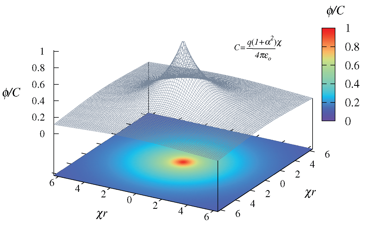
Figure 2.
Measured (circles) and calculated (rectangles) values of the muon anomalous g-factor. The numerical representation of the most recent data is given in Table 1.
Figure 2.
Measured (circles) and calculated (rectangles) values of the muon anomalous g-factor. The numerical representation of the most recent data is given in Table 1.
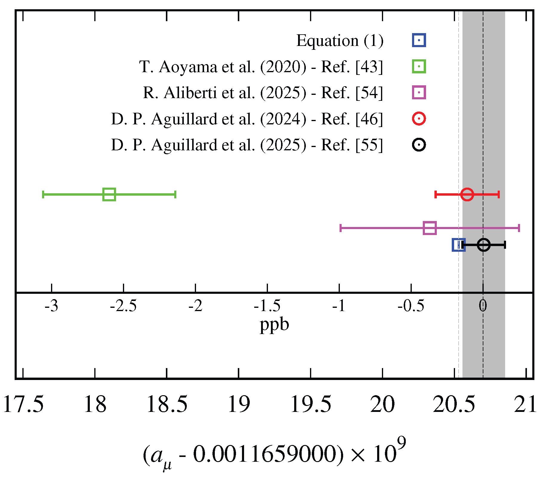
Figure 3.
Experimental (circles) and calculated (rectangles) data for the electron’s anomalous g-factor. The uncertainty in the theoretical results is related only to the corresponding value of fine-structure constant.
Figure 3.
Experimental (circles) and calculated (rectangles) data for the electron’s anomalous g-factor. The uncertainty in the theoretical results is related only to the corresponding value of fine-structure constant.
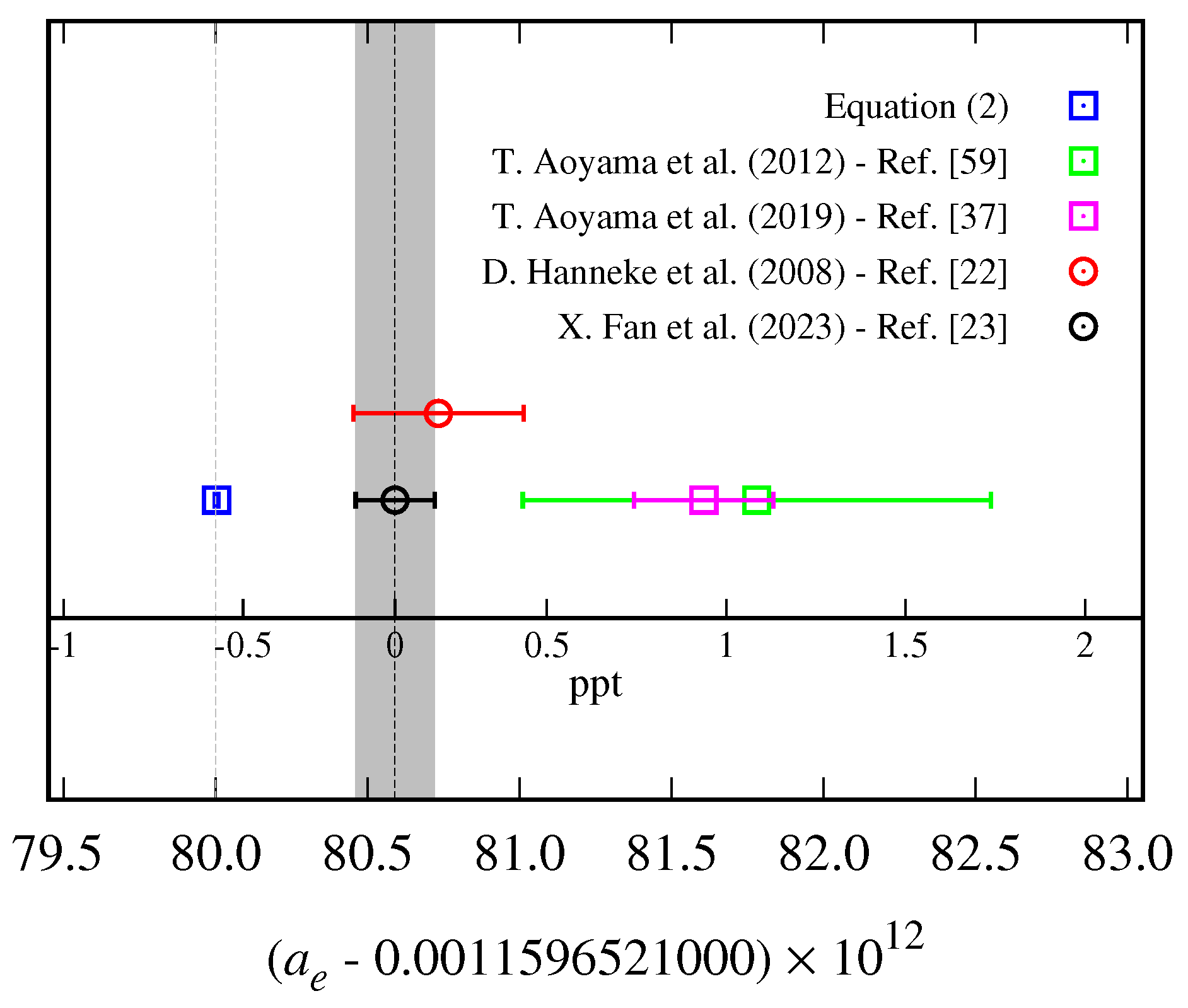
Figure 4.
Geometric representation of the spin angular momentum dynamics. (a) Sketch of precessing about the axis of propagation spin angular momentum given in Equation (18). The respective helicity is positive. (b) Exposition of the corresponding right circularly polarized transverse spin component along with the two plane projections representing plane waves.
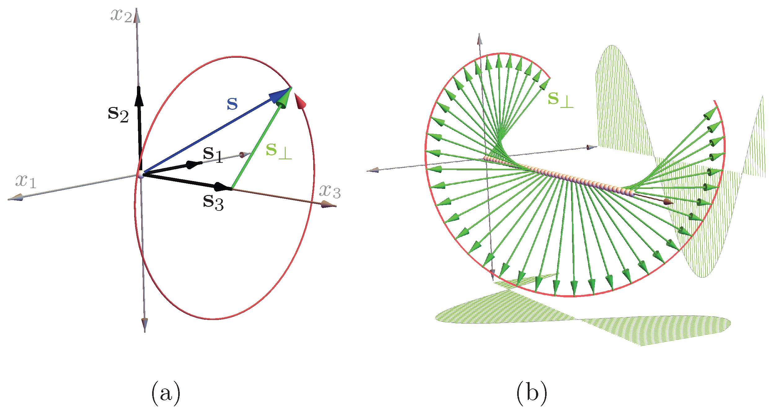

Table 1.
Comparison between the most recent theoretical (second and third rows) and experimental (fourth row) values of the muon’s anomalous g-factor. The listed values are depicted in Figure 2. The first uncertainty given in the second row is due to the fine structure constant and the second one is related only to the value of . Discussion is provided in Section 2.2.
| Approach | Reference | |
|---|---|---|
| Exact | Equation (1) | |
| SM | R. Aliberti et al. [54] | |
| FNAL (Run-1-6) | D. P. Aguillard et al. [55] |
Disclaimer/Publisher’s Note: The statements, opinions and data contained in all publications are solely those of the individual author(s) and contributor(s) and not of MDPI and/or the editor(s). MDPI and/or the editor(s) disclaim responsibility for any injury to people or property resulting from any ideas, methods, instructions or products referred to in the content. |
© 2025 by the authors. Licensee MDPI, Basel, Switzerland. This article is an open access article distributed under the terms and conditions of the Creative Commons Attribution (CC BY) license (http://creativecommons.org/licenses/by/4.0/).
Copyright: This open access article is published under a Creative Commons CC BY 4.0 license, which permit the free download, distribution, and reuse, provided that the author and preprint are cited in any reuse.


