
Submitted:
29 November 2025
Posted:
01 December 2025
You are already at the latest version
Abstract
Anomaly detection in safety-critical systems often operates under severe label constraints where only a small subset of normal and anomalous samples can be reliably annotated, while large unlabeled data streams are contaminated and high-dimensional. Deep one-class methods, such as deep support vector data description (DeepSVDD) and deep semi-supervised anomaly detection (DeepSAD), address this setting. However, they treat samples largely in isolation and do not explicitly leverage the manifold structure of unlabeled data, which can limit robustness and interpretability. This paper proposes Anomaly-Aware Graph-based Semi-Supervised Deep Support Vector Data Description (AAG-DSVDD), a boundary-focused deep one-class approach that couples a DeepSAD-style hypersphere with a label-aware latent k-nearest neighbor (k-NN) graph. The method combines a soft-boundary enclosure for labeled normals, a margin-based push-out for labeled anomalies, an unlabeled center-pull, and a k-NN graph regularizer on the squared distances to the center. The resulting graph term propagates information from scarce labels along the latent manifold, aligns anomaly scores of neighboring samples, and supports sample-level explanations through graph neighborhoods, while test-time scoring remains a single distance-to-center computation. On a controlled two-dimensional synthetic dataset, AAG-DSVDD achieves a mean F1-score of 0.88±0.02 across ten random splits, improving on the strongest baseline by about 0.12 absolute F1. In a multi-sensor fire monitoring case study, AAG-DSVDD reduces the average fire starting time accuracy to approximately 473 seconds (about 30% improvement over DeepSAD), while keeping the average pre-fire false-alarm rate below 1% and avoiding persistent pre-fire alarms. These results indicate that graph-regularized deep one-class boundaries offer an effective and interpretable framework for semi-supervised anomaly detection under realistic label budgets.
Keywords:
deep support vector data description (Deep SVDD)
; graph-based manifold regularization
; multi-channel time-series anomaly detection
; multi-sensor fire monitoring
; semi-supervised anomaly detection
MSC: 68T07; 68T05; 68T09
1. Introduction
The detection of anomalies constitutes a fundamental challenge in machine learning. It supports a wide range of applications, including process fault detection in industrial manufacturing [1], detection of cardiac abnormalities from ambulatory ECG recordings [2], intrusion detection in cybersecurity for networked infrastructures [3], and early fire detection in complex, non-fire environments using advanced SVDD-based monitoring [4]. The primary aim is to learn a compact representation of normal operating behavior and label deviations as anomalies, typically in the presence of severe class imbalance, where anomalous instances are rare and structurally diverse. In contrast to standard supervised classification, anomaly detection in real-world systems is usually limited by the available data and the scarcity of labels [5,6]. Acquiring accurate labels for normal and anomalous behavior can be expensive, hazardous, or practically impossible [7,8]. In many operational settings, certifying that a sample is truly normal requires expert review against process specifications, additional quality-control tests, or prolonged observation to rule out latent faults. In contrast, generating and labeling anomalies can require controlled stress tests, destructive experiments, or replay of hazardous conditions [7,8,9]. These constraints are particularly acute in safety-critical fire monitoring, where realistic fire scenarios must be conducted in specialized facilities with multi-sensor deployments, yielding only a modest number of labeled fire and non-fire sequences compared to the continuous stream of unlabeled sensor data observed during routine operation [10].
Classical work on one-class classification framed anomaly detection as the problem of estimating the support of normal data. Support vector data description (SVDD) represents the normal class by enclosing the mapped training examples within a minimum-radius hypersphere in feature space, classifying points that fall outside this sphere as anomalies [11]. In contrast, the one-class support vector machine (OC-SVM) learns a maximum-margin hyperplane that separates the mapped data from the origin, thereby implicitly characterizing the region of normal behavior [12]. Both approaches yield compact decision regions with a clear geometric interpretation, but they are usually trained on labeled normal samples and do not leverage the often-abundant pool of unlabeled observations present in many practical applications. When expert-validated normal labels are limited and expensive to obtain, while the majority of data arrive without labels, such supervised one-class methods can suffer from poor sample efficiency and instability.
The emergence of deep learning has driven substantial progress in anomaly detection. Deep one-class classification (DeepSVDD) builds on the SVDD framework by integrating a deep encoder that projects the data into a latent space, which is then bounded by a hypersphere [13]. Expanding on this concept, several deep SVDD extensions have been developed, including autoencoder-based approaches such as DASVDD [14], structure-preserving mappings that better retain neighborhood relationships [15], variational extensions leveraging VAE encoders [16], and contrastive learning objectives that enhance latent space representation and sharpen the decision boundary [17]. Deep semi-supervised anomaly detection (DeepSAD) extends this approach by leveraging a limited number of labeled anomalous samples to guide the deep one-class decision boundary when large amounts of unlabeled data are available [7]. In parallel, autoencoders and their extensions have been extensively employed to learn compact latent embeddings and reconstruction-based anomaly scores in industrial and temporal data scenarios [18,19], whereas self-supervised anomaly detection utilizes contrastive learning and related pretext objectives to improve representations when labeled data are scarce [20,21]. Nevertheless, a large proportion of deep anomaly detection approaches still rely on surrogate training objectives—such as reconstruction losses or generic self-supervised losses—that are only indirectly aligned with the final decision boundary, and typically incorporate unlabeled data through proxy tasks instead of imposing task-specific constraints directly on the boundary learner [22,23,24]. In addition, the resulting decision mechanisms are often difficult to interpret or connect to the underlying domain structure, which is a crucial limitation in safety-critical settings [25,26,27].
In safety-critical fire monitoring applications, there has been a growing reliance on machine learning methods applied to multi-sensor data streams obtained from temperature, smoke, gas, and particulate sensors. Gas-sensor array platforms employing multivariate calibration in combination with pattern-recognition algorithms have shown the capability to identify early-stage fires while compensating for sensor drift [28]. In indoor settings, researchers have investigated deep multi-sensor fusion by employing lightweight convolutional neural networks applied to fused temperature, smoke, and carbon monoxide (CO) signals [29]. Concurrently, transfer-learning frameworks have been introduced to adjust models originally trained in small-scale environments for application in larger rooms equipped with distributed multi-sensor nodes, thereby enhancing early detection capabilities across diverse deployment scenarios [30]. Complementary approaches based on signal processing and one-class modeling include a wavelet-based multi-modeling framework that learns separate detectors tailored to specific fire scenarios in multi-sensor settings [10]. In related work, a multi-class SVDD equipped with a dynamic time warping kernel has been proposed to distinguish among several fire and non-fire classes in sensor networks [4]. However, these sensor-driven frameworks are typically trained in a fully supervised regime at the window level, under the assumption that every time window is labeled as fire or non-fire. In practical deployments, obtaining such labels requires expensive and hazardous staged experiments in dedicated facilities that yield only a limited set of observations. Meanwhile, deployed multi-sensor systems continuously generate large volumes of unlabeled time-series data during normal operation.
Graph-based semi-supervised learning provides a principled way to exploit unlabeled data by constructing a similarity graph over samples and enforcing smoothness of labels or scores along its edges. Classical formulations such as Gaussian fields and harmonic functions and manifold regularization encode the cluster assumption through graph Laplacians that penalize rapid variation between neighboring nodes [31,32]. In the context of anomaly detection, graph-based methods have been explored at node, edge, and graph levels across a range of applications [33,34]. Within the SVDD framework, graph-based semi-supervised SVDD augments the SVDD objective with a Laplacian term derived from a k-nearest neighbor (k-NN) spectral graph, thereby leveraging the structure present in unlabeled data [35]. Manifold-regularized SVDD generalizes this approach by incorporating a graph Laplacian regularization term, which enforces similar scores for neighboring samples and thereby enhances robustness against noisy labels [36]. In addition, a semi-supervised CNN–SVDD architecture integrates convolutional feature learning with an SVDD-based objective and graph-regularization terms to support industrial condition monitoring, such as wind-turbine health assessment [37].
Despite these advancements, considerable limitations persist in boundary-focused deep anomaly detection for high-dimensional and multi-channel time series when operating under realistic labeling constraints. DeepSAD introduces deep representations and, in principle, can leverage a limited set of labeled examples [7]. In its standard formulation, however, unlabeled data are incorporated primarily through point-wise loss terms applied to individual samples, without explicit interaction terms that capture relationships among unlabeled instances in latent space. As a result, the unlabeled data manifold or neighborhood structure is not directly reflected in the boundary-focused objective, which can limit the model’s ability to propagate information from the limited labeled set throughout the geometry of the unlabeled data. Moreover, existing DeepSAD-based studies have not systematically explored such semi-supervised, one-class formulations in safety-critical multi-channel monitoring applications in which labeled data are costly and hazardous to acquire, unlabeled data streams are abundant, and missed detections and false alarms carry substantial operational and safety risks [4,10,28,29,30]. These applications require not only strong detection accuracy, but also interpretable anomaly decisions, allowing the score associated with a specific unlabeled sample to be traced back to representative normal or abnormal patterns [25]. These gaps motivate extensions of DeepSAD that (i) preserve a boundary-focused one-class objective while explicitly modeling manifold interactions among unlabeled samples, (ii) directly link anomaly scores of neighboring samples by exploiting the latent-space geometry of unlabeled data, (iii) are specifically adapted to the semi-supervised, label-budget constraints typical of multi-channel sensor monitoring, and (iv) enable sample-level interpretability by associating unlabeled samples with nearby labeled normal and anomalous samples based on their neighborhood relations and similarity in anomaly scores.
Motivated by these challenges, this paper introduces Anomaly-Aware Graph-based Semi-Supervised Deep SVDD (AAG-DSVDD), a boundary-focused deep one-class method for high-dimensional and multi-channel time series under realistic label budgets. Specifically, we introduce a semi-supervised, center-based objective that maintains the DeepSVDD-style hypersphere formulation, while explicitly modeling manifold relationships among unlabeled samples through a graph constructed from their squared distances to the center. AAG-DSVDD constructs a label-aware k-NN graph in the latent space that preferentially connects unlabeled samples to reliable labeled neighbors and couples their anomaly scores through graph regularization. This design allows information from the limited labeled set to propagate along the manifold structure of the unlabeled data. The resulting graph structure and latent representation further support sample-level explanations, as anomaly scores for unlabeled samples can be related back to nearby labeled normal and anomalous samples through their neighborhood relations and score similarities. Finally, we evaluate the proposed approach on both a controlled synthetic dataset and a real multi-sensor fire-monitoring case study under semi-supervised label-budget constraints. To the best of our knowledge, this constitutes the first AAG-DSVDD application to semi-supervised multi-sensor fire detection. On the synthetic benchmark, AAG-DSVDD achieves higher overall F1 scores than classical SVDD/SVM and deep anomaly detection baselines, indicating more accurate separation between normal and anomalous samples. In fire monitoring, the experimental results demonstrate faster fire-event detection and competitive false-alarm rates compared to these baselines.
The remainder of this paper is organized as follows. Section 2 introduces the problem setting and DeepSAD. Section 3 presents the proposed AAG-DSVDD approach. Section 4 describes the experimental setup and results on a controlled synthetic dataset. Section 5 reports the multi-sensor fire-monitoring case study under semi-supervised label-budget constraints. Finally, Section 6 concludes the paper and outlines directions for future work.
2. Background and Problem Formulation
In this section, we formalize the semi-supervised anomaly detection setting considered in this work, introduce the notation used throughout the paper, and present the DeepSAD objective that serves as our baseline. We then discuss the limitations of DeepSAD in leveraging the geometry of unlabeled data and motivate the need for graph-based regularization.
2.1. Semi-Supervised Anomaly Detection Setting and Notation
Let denote the input space and the latent space induced by a parametric encoder
where collects the weight matrices of all layers in the encoder network. For an input vector , we write
for its latent representation.
We consider a semi-supervised one-class anomaly detection setting in which only a small subset of samples is labeled, while the remaining majority is unlabeled and may contain both normal and anomalous instances. Formally, the training data consist of three subsets: a set of labeled normal samples
a set of labeled anomalous samples
and a set of unlabeled samples
We use the convention for labeled normal samples, for labeled anomalous samples, and for unlabeled samples. We denote the numbers of observations by , , and for , , and , respectively, and write for the total number of training observations.
The objective of one-class anomaly detection is to learn a decision function that assigns an anomaly score to each sample, where larger scores indicate stronger evidence of anomalous behavior. A threshold on then yields binary anomaly decisions. In center-based one-class models, the decision function is defined through distances to a learned center . Specifically, for each sample we define its latent representation and its squared Euclidean distance to the center
The scalar serves as the core anomaly score, optionally combined with a learned radius to form a decision rule such as “normal if ” and “anomalous otherwise”.
In the semi-supervised setting considered here, the goal is to learn the encoder parameters W and the center vector (and, if used, the radius R) from the labeled and unlabeled training data such that labeled normals are mapped close to the center, labeled anomalies are mapped far from the center, and unlabeled points are taken into account in a way that is robust to possible contamination and that exploits their geometric structure in latent space.
2.2. Overview of DeepSAD
DeepSAD extends DeepSVDD to the semi-supervised setting by adding a label-dependent term for a small set of labeled examples while maintaining the same center-based hypersphere structure in latent space [7].
Using the notation from Section 2.1, we define the set of all labeled observations as and note that it contains samples, while contains unlabeled samples, with in total. The DeepSAD loss can then be written in our notation as the following optimization problem over W:
The first term in (1) is exactly the DeepSVDD loss applied to the unlabeled data, encouraging all unlabeled samples to lie close to the center in latent space. The second term is the semi-supervised extension: for labeled normals in with , the exponent yields
which reduces to a standard squared-distance penalty and encourages these samples to be mapped close to the center . For labeled anomalies in with , the exponent yields
an inverse squared-distance penalty that is minimized by pushing these samples far away from the center. The scalar controls the relative weight of the labeled term relative to the unlabeled term, while is the strength of the weight decay applied to the weight matrices via the Frobenius norms .
The anomaly score for any sample is defined as the Euclidean distance of its latent representation to the center,
A threshold on is then used to distinguish normal and anomalous samples. DeepSAD therefore preserves the center-based one-class decision mechanism while incorporating label information through the exponentiated term for and the weighting parameter , in combination with the unlabeled DeepSVDD term.
2.3. Limitations of DeepSAD and Need for Graph-Based Regularization
Although DeepSAD is a flexible and effective framework for semi-supervised anomaly detection, its objective in (1) remains fundamentally point-wise: each sample contributes to the loss only through its own distance and, for labeled samples, its own label . The unlabeled term aggregates individual squared distances for , and the labeled term aggregates squared distances raised to the label exponent for , but there are no interaction terms coupling different samples or encoding a neighborhood graph, local density, or manifold structure in latent space. Consequently, unlabeled data influence the model only indirectly through penalties on individual points, rather than through constraints that explicitly relate nearby samples.
This strictly point-wise approach also restricts how information from the small labeled subset can spread into the unlabeled pool. In realistic semi-supervised settings, both labeled normal and anomalous examples are scarce, whereas unlabeled data densely occupy the regions in which a robust decision boundary must be learned. Ideally, unlabeled instances lying in areas dominated by labeled normals should naturally acquire lower anomaly scores, while those residing close to labeled anomalies should be driven toward higher scores. In DeepSAD, such behavior can only arise indirectly through the shared encoder parameters W; there is no explicit mechanism that couples the anomaly scores of nearby points or enforces consistency along the underlying data manifold.
Moreover, the absence of an explicit structure over samples constrains interpretability. DeepSAD provides a scalar anomaly score for each sample through its distance to the center, but it does not reveal how a given unlabeled sample is positioned relative to nearby labeled normals and anomalies in latent space. For many safety-critical applications, it is desirable not only to identify an observation as anomalous, but also to relate this decision to representative neighboring patterns that support or contextualize the score.
Taken together, these limitations motivate the incorporation of an explicit neighborhood structure into the DeepSAD framework, so that label information can propagate along the data manifold and anomaly scores are encouraged to be locally consistent and more interpretable. In the next section, we introduce a DeepSAD variant that realizes this idea.
3. Anomaly-Aware Graph-Based Semi-Supervised Deep SVDD
In this section, we introduce AAG-DSVDD, a DeepSAD-style extension that preserves the center-based hypersphere geometry in latent space while explicitly exploiting the geometry of labeled and unlabeled data. The method combines (i) a soft-boundary enclosure on labeled normals, (ii) a margin-based push-out on labeled anomalies, (iii) a center-pull on unlabeled samples, and (iv) a graph regularizer on the squared-distance field over a label-aware, locally scaled latent k-NN graph.
We retain the notation of Section 2.1: denotes an input vector, its latent embedding, a latent center, and the label indicating a labeled normal, unlabeled, or labeled anomalous sample, respectively. We write
for the squared distance of to the center, and we use the notation for the positive part of u.
3.1. Latent Encoder, Center, and Radius
The AAG-DSVDD model uses a deep encoder
implemented either as a multilayer perceptron (MLP) or as a long short-term memory (LSTM)-based sequence encoder [38] for multi-channel time series. For each input , we write
for its latent representation.
In the latent space, we maintain a center vector and a nonnegative radius . The squared distance of to the center is
These distances form the basis of both the training objective and the anomaly score at test time, with the sign of indicating whether an observation lies inside or outside the learned hypersphere. The practical initialization and updating of and R follow standard soft-boundary Deep SVDD practice and are detailed in Section 3.4.
3.2. Label-Aware Latent K-NN Graph with Local Scales
To exploit the geometry of the joint labeled–unlabeled sample, we construct a label-aware K-NN graph over latent embeddings with node-adaptive Gaussian weights. Let
denote the matrix of embeddings for all n training samples. For each node , we find its K nearest neighbors in latent space and denote their indices by , using Euclidean distance in and recording the corresponding distances .
We assign each node a local scale from the empirical distribution of its neighbor distances. Concretely, we compute the median of the nonzero distances in and use it as a robust estimate of the local density scale. This yields a self-tuning, node-adaptive Gaussian affinity
in the spirit of locally scaled kernels for spectral clustering [39]. Using in the denominator adapts the effective kernel width to the local density around both endpoints.
We then apply a label-aware edge policy. For nodes with (unlabeled), we retain all K nearest neighbors in irrespective of their labels. In contrast, when (labeled), we scan the neighbors of i in order of increasing distance and retain only those nodes j with (unlabeled), until K neighbors are selected or the candidate list is exhausted. This construction ensures that most outgoing edges from labeled points terminate in unlabeled nodes, allowing label information to propagate into the unlabeled pool while reducing the risk of overfitting to the sparse labeled set.
Let denote the resulting sparse affinity matrix, with for pairs that do not form edges. To keep the overall scale comparable across nodes of different degrees, we row-normalize W to obtain
and then construct a symmetrized affinity matrix
Finally, we define
a symmetric matrix that encodes the latent K-NN graph and will later be used through the quadratic form on the vector of squared distances .
3.3. Loss Components and Overall Objective
Let , , and denote the sets of labeled normals, labeled anomalies, and unlabeled samples, with cardinalities , , and , respectively. For each training sample we write for its latent embedding and
for its squared distance to the center. We collect these distances into the vector
Throughout this subsection we use the notation for the hinge operator, and we write hinge-type penalties with an exponent .
AAG-DSVDD combines four primary components: a graph-based regularizer on the squared-distance field, a soft-boundary enclosure on labeled normals, a margin-based push-out on labeled anomalies, and an unlabeled center-pull, together with a soft-boundary radius term and standard weight decay.
3.3.1. Graph Regularizer on Squared Distances
Using the symmetric matrix L defined in (5), which encodes the latent K-NN graph, we define a smoothness penalty on the squared distances as
where collects the squared distances . Since with M the normalized, symmetrized affinity matrix from Section 3.2, we can rewrite
For a given overall scale , minimizing is equivalent to maximizing . Because and is larger on pairs of nodes that are strongly connected in the latent K-NN graph, the term becomes large when neighboring nodes with high affinity carry similar squared distances. Thus, configurations in which varies smoothly over high-affinity regions of the graph are favored, whereas sharp changes in across strongly connected nodes tend to increase .
In effect, encourages neighboring samples in latent space to have compatible anomaly scores , allowing information from the limited labeled normals and anomalies to diffuse into the unlabeled pool.
3.3.2. Labeled-Normal Soft-Boundary Enclosure
For labeled normals , the model should treat the hypersphere of radius R as a soft boundary: most normal embeddings are expected to lie inside, while a small fraction of violations is tolerated. Using the squared distances , we penalize such violations through a hinge-type term
where denotes the hinge operator, is a soft-boundary parameter, and controls the curvature of the penalty. Only labeled normals with contribute to . When a normal sample lies inside the hypersphere (), its contribution is zero, whereas normals outside the boundary incur a positive loss that grows as . Normalizing by ensures that the penalty scales with the proportion of violating normals rather than their absolute count, so that the effective tightness of the hypersphere is controlled by , as in soft-boundary Deep SVDD [13], and not by the number of labeled normal samples. In particular, smaller values of correspond to a tighter enclosure (fewer tolerated violations), while larger values allow a greater fraction of labeled normals to lie near or beyond the boundary.
3.3.3. Labeled-Anomaly Margin Push-Out
For labeled anomalies , we enforce a clearance margin beyond the hypersphere:
where is an anomaly weight coefficient. This term is active only when an anomaly lies inside the hypersphere or within the margin region . Under such conditions, pushes its embedding farther from the center, either by increasing or, through the joint optimization, discouraging increases in that would otherwise encapsulate it.
3.3.4. Unlabeled Center-Pull
Unlabeled samples provide dense coverage of the data manifold but may contain contamination. To stabilize the global scale of the squared-distance field and keep the center anchored when is small, we apply a label-free pull-in on unlabeled distances:
This term reduces the mean of over the unlabeled pool toward , complementing the local smoothness imposed by . Its influence is controlled by a coefficient .
3.3.5. Overall Objective
Combining all components, the full AAG-DSVDD loss is
where scales the graph regularizer, controls the unlabeled center-pull, and is a weight-decay coefficient on the encoder parameters . The explicit term discourages unnecessarily large hyperspheres; together with and the soft-boundary radius update based on labeled normals, it yields behavior analogous to soft-boundary Deep SVDD, now coupled with anomaly margins, unlabeled pull-in, and graph-based smoothing. When and , the objective reduces to a soft-boundary Deep SVDD-like loss acting on labeled normals and labeled anomalies. Further setting recovers the standard soft-boundary Deep SVDD formulation on labeled normals alone.
The exponent shapes the hinge-type penalties in and . For , violations are penalized linearly, yielding piecewise-constant gradients whenever . For , the penalty is quadratic in the violation and the gradients scale linearly with its magnitude. In our experiments we use , which empirically produces smoother, magnitude-aware updates and improves training stability, particularly in the presence of scarce labels and the additional graph regularizer.
The different components of (10) interact to shape the decision boundary in a neighborhood-aware manner. The labeled-normal term and the radius R establish a soft hypersphere around that encloses most labeled normals and treats their squared distances as a reference scale for normal behavior. The anomaly margin term pushes labeled anomalies beyond by at least m, so that regions of latent space associated with anomalous patterns are encouraged to have larger and lie outside the hypersphere. The unlabeled center-pull stabilizes the global level of the squared-distance field when labeled normals are few, preventing uncontrolled drift of for unlabeled samples. Finally, the graph regularizer couples these effects along the latent K-NN graph by favoring configurations in which strongly connected neighbors have compatible squared distances. As a result, unlabeled samples that are well embedded in normal-dominated neighborhoods tend to inherit small and be enclosed by the decision boundary, whereas unlabeled samples whose neighborhoods are influenced by anomalies are pushed toward larger and are more likely to lie outside the hypersphere, receiving higher anomaly scores .
3.4. Optimization and Anomaly Scoring
The encoder parameters W and the soft-boundary radius R are optimized by stochastic gradient methods with mini-batch training, combined with periodic closed-form updates of and periodic reconstruction of the latent K-NN graph. This procedure follows standard Deep SVDD practice while incorporating the additional semi-supervised and graph-based terms in (10). In our implementation, training runs for epochs with mini-batches of size B.
We first perform a short warm-up phase on labeled normals in . During warm-up, the encoder is trained for a few epochs to minimize the average squared norm of the embeddings,
which stabilizes the latent representation around the origin. After the warm-up phase, we determine the center as the empirical average of the embeddings corresponding to the labeled normal samples,
and then keep fixed. We employ a block-coordinate strategy for the soft-boundary radius. Following the standard training procedure of the soft-boundary Deep SVDD [3,13], we do not backpropagate through R. Instead, we treat as a scalar quantity that is updated independently of the gradient-based optimization. Using the current distances of the labeled normal samples, we set
where denotes the empirical -quantile and controls the tolerated fraction of normal violations. During training, is held fixed within each epoch while W is updated, and after selected epochs we refresh by reapplying the same quantile rule to the current squared distances of labeled normals. In practice, this refresh is performed every epochs starting from a user-specified epoch . This yields a soft-boundary behavior in which roughly a fraction of normals may lie on or outside the hypersphere, matching the interpretation of in the original soft-boundary Deep SVDD formulation [13].
Within each epoch, we sample mini-batches of size B from the combined training set . For each mini-batch, we compute embeddings , squared distances , and the batch contributions of the labeled-normal, labeled-anomaly, and unlabeled terms , , and . The graph term is not evaluated at the mini-batch level. Gradients of the resulting mini-batch loss are backpropagated through the encoder parameters W, while and the graph matrix are treated as constants. We use the Adam optimizer [40] with weight decay to minimize (10) with respect to W for fixed .
To integrate the graph regularizer, we periodically reconstruct the label-aware latent K-NN graph using the current embeddings. At the start of each graph-refresh interval (every epochs), we first compute for all training samples, then rebuild the label-aware K-NN graph with local scaling, and finally construct the symmetric matrix L as defined in Section 3.2. This matrix L is kept fixed until the next refresh. During this interval, if , we perform a separate full-batch gradient update on the graph term based on the current embeddings, thereby updating W while keeping L unchanged. We do not backpropagate gradients through the graph construction process or the quantile updates of . Consequently, the optimization procedure alternates between mini-batch updates on the labeled and unlabeled objectives and occasional full-batch updates that smooth the squared-distance field over the latent K-NN graph.
Let denote the trained encoder parameters, radius, and center. For any test sample , we compute its anomaly score as the signed squared radial distance
By this convention, points outside the hypersphere have and are treated as anomalies, inliers satisfy , and boundary points satisfy . A decision threshold on is chosen on a held-out validation set, for example by targeting a desired false-alarm rate on validation normals or by maximizing a suitable detection metric. At test time, the graph is not required and AAG-DSVDD behaves as a standard center-based one-class model. Each input is processed by a single forward pass through to obtain its embedding, and the anomaly score is computed from the squared distance
The AAG-DSVDD algorithm is summarized in Algorithm 1. The scoring and decision rule are summarized in Algorithm 2.
The computational cost of the graph regularization is minimized by the locally connected structure of the label-aware latent k-NN graph. Although the graph matrix L has dimensions , it is mathematically sparse as each node is connected to at most k neighbors, and edges originating from labeled samples are further restricted to connect only to unlabeled neighbors. Consequently, the number of non-zero entries in L scales linearly with n rather than quadratically. This allows the graph regularization term to be evaluated in operations. Furthermore, the neighbor search—typically with spatial indexing—is amortized by performing the graph update only at intervals , independent of the encoder’s gradient iteration. Finally, it is important to note that this graph structure is used solely for regularization during training. At test time, the model requires only a single forward pass through the encoder to compute the distance to the center, thereby maintaining the fast inference speed of the standard DeepSVDD and DeepSAD.
| Algorithm 1: AAG-DSVDD (training) |
|
Inputs: , , , encoder , hyperparameters , training schedule , Adam optimizer with weight decay .
Outputs: , , .
Initialization:
Epoch loop: For :
Return:.
|
| Algorithm 2: AAG-DSVDD scoring and optional threshold selection |
|
3.5. Calibration of AAG-DSVDD Hyperparameters
The hyperparameters of AAG-DSVDD fall into three main groups, namely encoder capacity, loss weights, and graph construction. Encoder choices such as latent dimension, hidden sizes, and depth control how expressive is.
The loss coefficients directly shape the decision boundary. The soft-boundary parameter has the same role as in soft-boundary Deep SVDD. Smaller values enforce a tighter hypersphere around labeled normals. The anomaly weight and the margin m determine the strength and extent to which labeled anomalies are pushed away from the center. Larger values emphasize separation, but they can overreact to a small number of anomaly labels.
The unlabeled weight determines how much the unlabeled pool pulls the center and the radius. High lets the boundary track the overall unlabeled distribution, which is useful when contamination is low. Low keeps the model closer to a purely labeled one-class setting. The graph weight scales the smoothness penalty on squared distances over the latent K-NN graph. Larger propagates supervision more strongly along the manifold but may oversmooth the boundary. Smaller limits geometric coupling.
The neighborhood size K controls graph density and the scale of smoothing. Larger K yields broader and more global regularization. Smaller K produces more localized and fine-grained boundaries. In practice, we tune scalar coefficients such as and m on logarithmic grids. We select K, the latent dimension, and the network depth from small discrete sets using validation performance.
4. Experiments on Synthetic Data
We first study AAG-DSVDD in a controlled two-dimensional setting, where the geometry of normals, anomalies, and the learned decision boundary can be visualized. We compare AAG-DSVDD against DeepSVDD [13], DeepSAD [7], OC-SVM with a radial basis function (RBF) kernel (OC-SVM) [12], and classical SVDD with an RBF kernel (SVDD-RBF) [11]. All methods operate in the same semi-supervised setting, where only a small fraction of the training normals and anomalies are labeled and the remaining training points form a contaminated unlabeled pool.
4.1. Synthetic Dataset Description
We generate a two-dimensional dataset with a curved normal manifold and off-manifold anomalies. Normal samples are obtained by first drawing a Gaussian vector with diagonal covariance and then applying a quadratic bending transform
followed by global scaling and the addition of small Gaussian noise. The parameters are set to , , bend , and noise level . This procedure produces a nonlinearly curved, banana-shaped normal region.
Anomalies are drawn from a mixture of two Gaussian distributions located above and below the banana. Concretely, half of the anomalous points are sampled from
and the remaining half from
with small Gaussian noise added. In all experiments we generate normal points and 800 anomalies, for a total of observations in .
The synthetic dataset is randomly partitioned at the observation level into training, validation, and test sets. We reserve of the data as a test set and as a validation set, using stratified sampling so that the proportions of normal and anomalous points are preserved in each split. The remaining of the data form the training set. Within this training set, we construct a semi-supervised labeling scheme by retaining of the training normals as labeled normals with and of the training anomalies as labeled anomalies with . All remaining training points are treated as unlabeled with . This results in a setting where only a small subset of both classes is labeled, while the unlabeled pool contains a mixture of normals and anomalies, replicating realistic contamination in semi-supervised anomaly detection. The same splits and label budgets are used for all methods to ensure a fair comparison. A sample training dataset from an experiment is shown in Figure 1.
4.2. Baselines, Architectures, and Hyperparameters
All deep methods use the same bias-free multilayer perceptron encoder for fairness. The encoder maps to a 16-dimensional latent space through two hidden layers of sizes 256 and 128 with ReLU activations. We train all deep models with the Adam optimizer for 50 epochs, mini-batches of size 128, and learning rate . The weight decay is set to for AAG-DSVDD and for DeepSVDD and DeepSAD. The anomaly class is treated as the positive class in all evaluations.
For AAG-DSVDD we use the soft-boundary formulation of Section 3 with squared hinges (), soft-boundary parameter , anomaly weight , and margin . The unlabeled center-pull weight is set to , and the graph smoothness weight to , which provides a moderate level of graph-based regularization. The latent K-NN graph uses neighbors with the locally scaled Gaussian affinities of Section 3.2. The radius update schedule and graph-refresh schedule follow Section 3.4, with quantile-based updates of at level and reconstruction of the latent K-NN graph every two epochs.
DeepSVDD uses the same encoder architecture and soft-boundary parameter but is trained on labeled normals only, following the standard one-class setup. It omits anomaly margins, unlabeled pull-in, and graph regularization. DeepSAD is instantiated with the same encoder and optimizes the semi-supervised DeepSAD objective on the same labeled and unlabeled splits, with labeled-term weight . Unlabeled points contribute through the DeepSAD loss. Both AAG-DSVDD and DeepSAD exploit labeled anomalies, whereas DeepSVDD does not.
OC-SVM and SVDD-RBF are trained on the same training normals (ignoring anomaly labels) with an RBF kernel and . OC-SVM uses the scale heuristic for the kernel width (included in the scikit-learn OC-SVM library), while SVDD-RBF uses a fixed kernel width parameter . These methods serve as classical non-deep one-class baselines with fixed kernels in the input space, in contrast to the learned latent geometry of the deep methods.
4.3. Evaluation Metrics
All methods output an anomaly score , with larger values indicating more anomalous points. For AAG-DSVDD we use the signed squared radial distance
DeepSVDD and DeepSAD use their standard distance-based scores in latent space, which have the same form up to the learned center and radius. For OC-SVM and SVDD-RBF we use their native decision functions, with signs adjusted where necessary so that higher values correspond to a higher degree of abnormality.
For each method and each random seed, we select a decision threshold on the validation set by scanning candidate thresholds and choosing the one that maximizes the F1-score on the validation split. On the held-out test set, an observation is then classified as anomalous if and normal otherwise. The anomaly class is treated as the positive class in all evaluations.
Given the resulting binary predictions, we compute the confusion counts (true positives), (false positives), (true negatives), and (false negatives) on the test set. From these we report precision, recall, F1-score, and accuracy:
To assess robustness to random initialization and sampling, we repeat the entire procedure over ten random seeds . For each method we summarize performance by reporting the mean and standard deviation of the test F1-score across these seeds.
4.4. Results and Analysis
The performance comparison of the methods on the synthetic banana dataset is given in Table 1 and Table 2. Table 1 presents the performance of the methods in an experiment conducted on the synthetic banana dataset. AAG-DSVDD achieves the best performance on three metrics. It reaches an F1 score of 0.89 and an accuracy of 0.91. Its recall is 0.90, which is slightly lower than DeepSAD at 0.98, but AAG-DSVDD maintains a much higher precision of 0.87 compared to 0.49 for DeepSAD. DeepSVDD, OC-SVM, and SVDD-RBF also show imbalanced tradeoffs between recall and precision. DeepSAD and DeepSVDD favor recall and allow many false alarms on normal samples, reducing their F1 scores and accuracies. OC-SVM and SVDD-RBF improve precision relative to deep one-class baselines but still fall short of AAG-DSVDD in F1, recall, and accuracy.
Table 2 examines robustness in ten independent runs with different random seeds. AAG-DSVDD consistently achieves the highest F1 score, with a mean of 0.88 and a standard deviation of 0.02. The strongest baseline is SVDD-RBF, with a mean F1 of 0.76 and a standard deviation of 0.04. OC-SVM, DeepSVDD, and DeepSAD achieve mean F1 scores of 0.71, 0.62, and 0.65, respectively, with moderately greater variability. The paired t-tests and the Wilcoxon signed-rank tests in the bottom rows of Table 2 compare each baseline with AAG-DSVDD under the one-sided alternative that AAG-DSVDD has a higher F1. All t-test p-values are below and all Wilcoxon p-values equal . These results show that the improvements of AAG-DSVDD over each baseline are not only large in magnitude but also statistically significant across different random realizations of the dataset and the semi-supervised labels.
The decision boundaries obtained over an experiment are shown in Figure 2 for all the methods. These trends are consistent with how the different objectives use labels and geometry. DeepSVDD is trained only on labeled normals and fits a soft-boundary hypersphere in latent space. With few labeled normals, the learned region stays concentrated around the densest part of the data, so many legitimate normals in sparser areas are rejected as anomalies, which drives up false positives and reduces precision, accuracy, and F1. DeepSAD introduces labeled anomalies and an unlabeled term, but still relies on distances to a single center. In this setting, it tends to enlarge the decision region to recover anomalous points, which explains its very high recall but also its low precision.
OC-SVM and SVDD-RBF learn directly in the input space with fixed RBF kernels without representation learning or graph structure. They form smooth one-class boundaries around the global data cloud and achieve better precision than DeepSVDD and DeepSAD, yet they cannot adapt the feature space or exploit the unlabeled manifold structure, so they remain clearly dominated by AAG-DSVDD in F1 and accuracy. In contrast, AAG-DSVDD combines a DeepSVDD-style enclosure with a latent k-NN graph and anomaly-aware regularization. The graph term couples scores along the latent manifold so that unlabeled samples help stabilize the center and radius, while anomaly-weighted edges and push-out penalties move the boundary away from regions associated with anomalies. This produces a decision region that covers most normals and excludes anomaly clusters, consistent with the higher and more stable F1 scores observed for AAG-DSVDD in Table 1 and Table 2.
Note that all deep models in this comparison (DeepSVDD, DeepSAD, and AAG-DSVDD) produce one-class decision regions defined by a single hypersphere in latent space, with the radius set by the learned quantile on labeled normals. When these distance-based boundaries are visualized in the original input space (in Figure 2) after the nonlinear mapping of the encoder, the corresponding curves can appear highly curved or even disconnected, despite arising from a single hypersphere in the learned latent representation.
4.5. Effect of Graph Regularization Weight
To assess the impact of the graph regularizer, we varied on the synthetic banana dataset while keeping all other hyperparameters fixed. Figure 3 reports the resulting F1-score and precision. For small to moderate values (–), performance is stable as F1 remains around – and precision around –, indicating that the method benefits from graph-based smoothing but is not overly sensitive to the exact choice of in this range.
As increases beyond 1, both F1 and precision degrade monotonically. At the F1-score drops to about , and for very large regularization () it falls below , with a corresponding precision below . This pattern is consistent with an over-smoothing effect. Excessively strong graph regularization pushes squared distances toward locally uniform values, obscuring the boundary between normal and anomalous regions. Based on these results, we use in the main synthetic experiments, a robust trade-off between leveraging the latent graph and avoiding over-regularization.
5. Case Study: Anomaly-Aware Graph-Based Semi-Supervised Deep SVDD for Fire Monitoring
In this section, we present a case study that applies the proposed AAG-DSVDD framework to real multi-sensor fire monitoring data. The goal is to detect the onset of hazardous fire conditions as early as possible while maintaining a low false-alarm rate. We first describe the fire monitoring dataset and its preprocessing. We then detail the semi-supervised training protocol, baselines, and evaluation metrics used to assess detection performance in this realistic setting.
5.1. Fire Monitoring Dataset Description
We evaluate the proposed method on a multi-sensor residential fire detection dataset derived from the National Institute of Standards and Technology (NIST) “Performance of Home Smoke Alarms” experiments [41]. In these experiments, a full-scale residential structure was instrumented and subjected to a variety of controlled fire and non-fire conditions. Sensor responses were recorded over time in systematically designed scenarios.
In our setting, each scenario is represented as a five-channel multivariate time series sampled at 1 Hz. At each time step t in scenario s, the observation vector contains measurements from five sensors in the following order. The first channel is a temperature sensor. The second channel measures CO concentration. The third channel records the output of an ionization smoke detector. The fourth channel records the output of a photoelectric smoke detector. The fifth channel measures smoke obscuration. Accordingly, each scenario s is stored as a matrix
where denotes the duration of that scenario in seconds.
The dataset comprises multiple classes of fire scenarios. These include smoldering fires, such as the smoldering of upholstery or mattress experiments. They also include cooking-related heating and cooking fires and flaming fires. For each fire scenario, a true fire starting time (TFST) is annotated. This TFST indicates the earliest time at which the fire is deemed to have started based on the original NIST records and the observed sensor responses. Table 3 shows the description of the fire scenarios.
To build intuition about the multi-sensor fire dynamics, Figure 4 shows an excerpt from one fire scenario (Scenario 4 in Table 3). The plots show the five sensor channels sampled at 1 Hz: temperature (top), CO concentration, ionization smoke, photoelectric smoke, and smoke obscuration (bottom). The vertical dotted line marks the annotated s.
Before TFST, all channels remain close to their baseline levels, with only small fluctuations attributable to noise. Shortly after TFST, the smoke obscuration begins to rise, followed by increases in the photoelectric and ionization detector outputs, and then a delayed but pronounced growth in CO concentration and temperature. This sequence reflects the physical development of the fire and highlights the temporal coupling between channels. It also motivates the use of windowed multi-channel inputs and a boundary-focused model that leverages the joint evolution of these signals rather than relying on any single sensor in isolation.
5.2. Window Construction and Experiment Setup
5.2.1. Sliding-Window Observations
We adopt a sliding-window observation structure similar to that used in previous real-time fire detection studies on this dataset. For each fire scenario s, let denote the five-dimensional sensor vector at second t, ordered as temperature, CO concentration, ionization detector output, photoelectric detector output, and smoke obscuration. We form an observation window of length w at time t as
where w is the window length in seconds. Each scenario s thus produces a sequence of windows .
For each fire scenario s, an annotated is given in seconds. We assign a binary label to each window based on the time of its last sample relative to this TFST. If the last time index of the window satisfies , the window is labeled as fire, and we set . If the window ends strictly before the fire starts, that is, , the window is labeled as normal, and we set . These end-of-window labels form the base labels on which we build the semi-supervised setting in the next subsection.
For notational consistency with Section 2.1, we subsequently denote each window by and its binary label by . When we use an LSTM encoder, is treated as an ordered length multivariate time series w in . For methods that require fixed-length vector inputs, such as OC-SVM and kernel SVDD, we additionally define a flattened version with by stacking the entries of along the time and channel dimensions into a single vector.
5.2.2. Experiment Setup
We construct an LSTM-ready dataset of five-channel windows with separate training, validation, and test splits. The training set is derived from four fire scenarios (1, 2, 3, and 4). From each of these scenarios, we sample fixed-length windows of size s using the sliding-window construction described in Section 5.2.1. In each training scenario, we draw approximately 250 windows, with about 40% taken from the pre-TFST region and labeled as normal, and about 60% taken from the post-TFST region and labeled as fire. This yields roughly 100 normal and 150 fire windows per training scenario, for a total of 1000 training windows across all four scenarios. In all cases, the binary label of a window is determined by the label at its last time step. For a semi-supervised setting, we randomly retain 10% of normal and fire windows as labeled samples, while the rest are considered unlabeled.
For evaluation, we generate dense sliding windows of length s with unit stride over complete scenarios. The validation windows are drawn from the same four scenarios (1, 2, 3, and 4), using all overlapping windows rather than the subsampled training set. The test windows are drawn from six additional fire scenarios (5, 6, 7, 8, 9, and 10) that do not appear in the training set. In all splits, a window is labeled as normal if its last time step occurs before the annotated for that scenario and as fire otherwise.
During the evaluation, each window is passed through the encoder and the AAG-DSVDD model to obtain an anomaly score . A window is classified as fire when its score exceeds a global threshold , which is selected using held-out validation windows from training scenarios. A scenario-level fire alarm is raised once consecutive windows are classified as fire. The estimated fire starting time (EFST) is defined as the time at which the model predicted a fire for q consecutive windows.
5.2.3. Evaluation Metrics
For each fire scenario s we obtain a sequence of ground-truth window labels
and the corresponding predicted labels
where is the number of windows in that scenario and denotes a predicted fire window.
For each scenario s, the is provided by the dataset annotation and expressed in window indices. Equivalently, it can be written as the first time point at which the ground-truth label becomes fire,
Given the predicted labels , we declare that a scenario-level fire alarm has been raised once q consecutive windows are classified as fire. In our experiments we use . The is defined as the last index of the first run of q consecutive fire predictions, that is,
This matches the implementation in which the alarm time is the index of the last window in the first run of q consecutive predicted fires.
The Fire Starting Time Accuracy (FSTA) for scenario s measures the temporal deviation of the estimated start time from the true start time. It is defined as the absolute difference between the estimated and true fire starting times:
By this definition, quantifies the magnitude of the error in seconds, treating early false alarms () and late detections () symmetrically. Lower values indicate better performance.
To quantify false alarms in the pre-fire region, we compute the false alarm rate (FAR) for each scenario with an annotated . Let
denote the set of pre-fire window indices. The per-scenario false alarm rate is
that is, the fraction of pre-TFST windows that are incorrectly classified as fire. In the reported tables we express as a percentage.
5.2.4. Model Architectures and Hyperparameters
All deep methods share the same LSTM-based encoder for fairness. Each input window is a sequence in with and five sensor channels. We use an LSTM encoder with input size 5, hidden size 128, two layers, no bi-directionality, and dropout set to zero. Its last hidden state is projected to a 64-dimensional representation. All deep models are trained with Adam for 50 epochs, batch size 256, and learning rate . The weight decay is for AAG-DSVDD and for DeepSVDD and DeepSAD. Fire windows are treated as positive classes in all evaluations. Alarm logic uses consecutive fire windows to declare a fire at the scenario level.
For AAG-DSVDD we use the soft-boundary formulation of Section 3 with squared hinges (), soft-boundary parameter , anomaly weight , and margin . The unlabeled center-pull weight is , and the graph smoothness weight is , which imposes strong graph regularization. The latent K-NN graph uses neighbors with the locally scaled Gaussian affinities of Section 3.2. The radius update and graph-refresh schedules follow Section 3.4, with quantile-based updates of at level and reconstruction of the latent K-NN graph every two epochs. The warm-up phase for center initialization runs for two epochs.
DeepSVDD uses the same encoder and MLP head and the same soft-boundary parameter . It is trained only on labeled normal windows and does not use anomaly margins, unlabeled pull-in, or graph regularization. DeepSAD also uses the same architecture and optimizes the standard semi-supervised DeepSAD objective on the same labeled and unlabeled splits, with labeled-term weight . In both AAG-DSVDD and DeepSAD, of normal windows are labeled normals and of fire windows are labeled anomalies. DeepSVDD uses only the labeled normal subset.
OC-SVM and SVDD-RBF are trained on flattened windows. Each window is reshaped into a 160-dimensional vector, and only labeled normal windows are used for training. Both methods use an RBF kernel with . For OC-SVM, we set the kernel width parameter to , while for SVDD-RBF, we use . These classical one-class baselines operate directly in the input space and provide a non-deep comparison to the LSTM-based models.
5.3. Fire Monitoring Results and Analysis
The per-scenario fire detection results for all methods are summarized in Table 4. For each test scenario we report the , the , the in seconds, and the . By construction of the EFST metric, if , then it indicates that the method has raised a false alarm. In contrast, if is equal to the duration of the scenario, the method never produces q consecutive fire predictions before the scenario ends and therefore fails to raise any stable fire alarm.
SVDD-RBF is extremely conservative. In all six test scenarios, its is exactly equal to the duration of the scenario. This means that it never detects a fire event at the level of a stable alarm. Therefore, the high FSTA values (from 209 s to 3487 s) reflect missed detections rather than late but successful alarms, which is in line with the average FAR for the SVDD-RBF being . OC-SVM moves in the opposite direction. On average, it reduces FSTA to about 215 s, but this comes at the cost of non-negligible pre-fire activity. The mean FAR is , and in the longest scenarios it is as high as (scenario 5) and (scenario 6). In these two scenarios, is smaller than . This indicates that OC-SVM raises false alarms well before the true fire onset. DeepSVDD achieves the second-smallest average FSTA (about 400 s) and detects the shorter flaming scenarios relatively quickly. However, it does so by triggering almost continuously in the pre-fire region. The average FAR is , and scenarios 5 and 6 both exhibit (an alarm essentially at the beginning of the scenario). Thus, the one-class baselines either miss fires altogether (SVDD-RBF) or raise persistently early alarms that would be unacceptable in a deployed monitoring system (OC-SVM and especially DeepSVDD).
The semi-supervised deep methods, DeepSAD and AAG-DSVDD, achieve a more favorable balance between timeliness and reliability. DeepSAD maintains a very low average FAR of , with at most in any scenario, but its timing behavior is mixed. In several scenarios (7, 8, 9, and 10), it produces moderate delays with FSTA between 100 and 170 s, while in scenario 5 it reacts extremely late (FSTA s). Moreover, in scenario 6 DeepSAD exhibits , which indicates that its first stable alarm is actually a false alarm in the pre-fire region, despite the low FAR reported there. In general, the mean FSTA for DeepSAD in all scenarios is about 689 s.
AAG-DSVDD yields the best overall trade-off. Across the six test scenarios, it reduces the mean FSTA to approximately 473 s, representing a substantial improvement over SVDD-RBF and a reduction of roughly relative to DeepSAD, while keeping the average FAR below (). Importantly, for AAG-DSVDD, we always have , so the first stable alarm in all scenarios occurs at or after the true onset of the fire. The gains are most pronounced in scenarios 5 and 9, where AAG-DSVDD triggers earlier than all baselines with negligible FAR, and in scenario 10, where it achieves the smallest FSTA of all methods (37 s) with zero pre-fire false alarms.
A critical observation from these results is the robustness of AAG-DSVDD against early false alarms, particularly when compared to the noisy behavior of DeepSVDD. DeepSVDD triggers almost continuously in the pre-fire regions of scenarios 5 and 6, suggesting that its decision boundary is overly sensitive to local fluctuations in the sensor noise floor. In contrast, the graph regularization in AAG-DSVDD explicitly enforces smoothness on the anomaly scores of neighboring latent representations. By coupling the scores of unlabeled pre-fire windows (which lie on the normal manifold) with those of the labeled normal set, the graph term effectively dampens high-frequency noise in the anomaly score trajectory. This smoothing effect prevents transient sensor spikes from crossing the decision threshold, resulting in a stable monitoring signal that only rises when the collective evidence from the multi-sensor array indicates a genuine departure from the normal manifold.
These results are consistent with the design of AAG-DSVDD. The baseline one-class models construct their decision regions using only sparsely labeled normals (and, for DeepSAD, a small number of labeled fires) and do not explicitly exploit the geometry of the unlabeled windows. Consequently, they tend either to tighten the normal region so aggressively that many pre-TFST windows are classified as anomalous, leading to , or to expand it so conservatively that no stable alarm is raised before the scenario ends, yielding .
In contrast, AAG-DSVDD regularizes the squared-distance field over a label-aware latent k-NN graph and couples labeled and unlabeled windows through its k-NN latent graph and unlabeled center-pull terms. This allows the model to propagate limited label information along the data manifold and to position the hypersphere boundary close to the true transition from normal to fire, resulting in earlier yet stable fire alarms with very few false activations on the NIST fire sensing dataset.
6. Conclusions and Future Work
This paper studied semi-supervised anomaly detection in high-dimensional and multi-channel time series under realistic label budgets and applied it to safety-critical fire monitoring. We proposed AAG-DSVDD, which preserves the center-based hypersphere structure of DeepSVDD/DeepSAD and augments it with a label-aware latent k-NN graph. By regularizing the squared-distance field over this graph and combining a soft-boundary term for labeled normals, a margin push-out for labeled anomalies, and an unlabeled center-pull, AAG-DSVDD propagates information from scarce labels along the latent manifold while retaining a simple distance-based decision rule at test time.
On the synthetic banana dataset, AAG-DSVDD consistently outperformed DeepSVDD, DeepSAD, OC-SVM, and SVDD-RBF. On the representative experiment, it achieved F1 and accuracy , compared with F1 and accuracy for the strongest classical baseline (SVDD-RBF) and F1 and accuracy for DeepSAD. Over ten seeds, AAG-DSVDD reached a mean F1 of versus for SVDD-RBF and for OC-SVM, with all gains statistically significant under paired tests. In the NIST-based fire monitoring case study, AAG-DSVDD reduced the mean fire starting time accuracy to about 473 s (about a 30% improvement over DeepSAD) while keeping the average pre-fire false-alarm rate below and ensuring that the first stable alarm in every scenario occurred at or after the true fire onset. Qualitatively, the decision boundaries learned by AAG-DSVDD track the true normal manifold more closely than the baselines, covering valid normal regions while cleanly and effectively detecting anomaly clusters. In the fire monitoring case study, its alarms align more closely with the physical development of the fire, avoiding the persistent false alarms of DeepSVDD and OC-SVM and the overly conservative behavior of SVDD-RBF, while still supporting sample-level explanations through its latent graph structure.
Beyond these quantitative gains, the latent graph provides a natural handle for interpretability, as anomaly scores of unlabeled samples can be related to nearby labeled normals and anomalies through their graph neighborhoods, while the final deployed model still operates via a single distance-to-center computation. As a promising direction for future work, the fixed Gaussian similarities on the latent graph can be replaced or complemented by attention-weighted graphs whose edge weights are learned end-to-end. Such attention-based graph constructions could adaptively emphasize informative neighbors and further improve robustness and detection quality under severe label scarcity and heterogeneous operating conditions.
Data Availability Statement
The raw data supporting the conclusions of this article will be made available by the authors on request.
Acknowledgments
The project was funded by KAU Endowment (WAQF) at King Abdulaziz University, Jeddah, Saudi Arabia. The authors, therefore, acknowledge with thanks WAQF and the Deanship of Scientific Research (DSR) for technical and financial support.
Conflicts of Interest
The authors declare no conflicts of interest
Abbreviations
The following abbreviations are used in this manuscript:
| Adam | Adaptive Moment Estimation |
| DeepSVDD | Deep Support Vector Data Description |
| DeepSAD | Deep Semi-Supervised Anomaly Detection |
| LSTM | Long Short-Term Memory |
| MLP | Multilayer Perceptron |
| OC-SVM | One-Class Support Vector Machine |
| RBF | Radial Basis Function |
| SVDD | Support Vector Data Description |
References
- Cai, L.; Yin, H.; Lin, J.; Zhou, H.; Zhao, D. A relevant variable selection and SVDD-based fault detection method for process monitoring. IEEE Transactions on Automation Science and Engineering 2022, 20, 2855–2865.
- Li, H.; Boulanger, P. A Survey of Heart Anomaly Detection Using Ambulatory Electrocardiogram (ECG). Sensors 2020, 20. [CrossRef]
- Alhindi, T.J. Severity-Regularized Deep Support Vector Data Description with Application to Intrusion Detection in Cybersecurity. Mathematics 2025, 13. [CrossRef]
- Alhindi, T.J.; Alturkistani, O.; Baek, J.; Jeong, M.K. Multi-class support vector data description with dynamic time warping kernel for monitoring fires in diverse non-fire environments. IEEE Sensors Journal 2025. [CrossRef]
- Chatterjee, A.; Ahmed, B.S. IoT anomaly detection methods and applications: a survey. Internet of Things 2022, 19, 100568. [CrossRef]
- Nassif, A.B.; Talib, M.A.; Nasir, Q.; Dakalbab, F.M. Machine learning for anomaly detection: A systematic review. IEEE Access 2021, 9, 78658–78700. [CrossRef]
- Ruff, L.; Vandermeulen, R.A.; Görnetz, N.; Binder, A.; Müller, E.; Müller, K.R.; Kloft, M. Deep semi-supervised anomaly detection. In Proceedings of the Proceedings of the International Conference on Learning Representations, 2020.
- He, Y.; Feng, Z.; Yan, T.; Zhan, Y.; Xia, Y. Meta-CAD: Few-shot anomaly detection for online social networks with meta-learning. Computer Networks 2025, 270, 111515. [CrossRef]
- Alhindi, T.J.; Baek, J.; Jeong, Y.S.; Jeong, M.K. Orthogonal binary singular value decomposition method for automated windshield wiper fault detection. International Journal of Production Research 2024, 62, 3383–3397. [CrossRef]
- Baek, J.; Alhindi, T.J.; Jeong, Y.S.; Jeong, M.K.; Seo, S.; Kang, J.; Shim, W.; Heo, Y. A wavelet-based real-time fire detection algorithm with multi-modeling framework. Expert Systems with Applications 2023, 233, 120940.
- Tax, D.M.J.; Duin, R.P.W. Support Vector Data Description. Machine Learning 2004, 54, 45–66.
- Manevitz, L.M.; Yousef, M. One-class SVMs for document classification. Journal of Machine Learning Research 2001, 2, 139–154.
- Ruff, L.; Vandermeulen, R.; Goernitz, N.; Deecke, L.; Siddiqui, S.A.; Binder, A.; Müller, E.; Kloft, M. Deep one-class classification. In Proceedings of the Proceedings of the International Conference on Machine Learning, 2018, pp. 4393–4402.
- Hojjati, H.; Armanfard, N. DASVDD: Deep autoencoding support vector data descriptor for anomaly detection. IEEE Transactions on Knowledge and Data Engineering 2024, 36, 3739–3750. [CrossRef]
- Zhang, Z.; Deng, X. Anomaly detection using improved deep SVDD model with data structure preservation. Pattern Recognition Letters 2021, 148, 1–6. [CrossRef]
- Zhou, Y.; Liang, X.; Zhang, W.; Zhang, L.; Song, X. VAE-based Deep SVDD for anomaly detection. Neurocomputing 2021, 453, 131–140. [CrossRef]
- Xing, H.J.; Zhang, P.P. Contrastive deep support vector data description. Pattern Recognition 2023, 143, 109820. [CrossRef]
- Pota, M.; De Pietro, G.; Esposito, M. Real-time anomaly detection on time series of industrial furnaces: A comparison of autoencoder architectures. Engineering Applications of Artificial Intelligence 2023, 124, 106597.
- Neloy, A.A.; Turgeon, M. A comprehensive study of auto-encoders for anomaly detection: Efficiency and trade-offs. Machine Learning with Applications 2024, 17, 100572.
- Tack, J.; Mo, S.; Jeong, J.; Shin, J. Csi: Novelty detection via contrastive learning on distributionally shifted instances. Advances in Neural Information Processing Systems 2020, 33, 11839–11852.
- Hojjati, H.; Ho, T.K.K.; Armanfard, N. Self-supervised anomaly detection in computer vision and beyond: A survey and outlook. Neural Networks 2024, 172, 106106.
- Chalapathy, R.; Chawla, S. Deep learning for anomaly detection: A survey. ArXiv Preprint arXiv:1901.03407 2019.
- Pang, G.; Shen, C.; Cao, L.; Hengel, A.V.D. Deep Learning for Anomaly Detection: A Review. ACM Computing Surveys 2021, 54. [CrossRef]
- Ruff, L.; Kauffmann, J.R.; Vandermeulen, R.A.; Montavon, G.; Samek, W.; Kloft, M.; Dietterich, T.G.; Müller, K.R. A unifying review of deep and shallow anomaly detection. Proceedings of the IEEE 2021, 109, 756–795.
- Li, Z.; Zhu, Y.; Van Leeuwen, M. A survey on explainable anomaly detection. ACM Transactions on Knowledge Discovery from Data 2023, 18, 1–54.
- Bouman, R.; Heskes, T. Autoencoders for Anomaly Detection are Unreliable. arXiv preprint arXiv:2501.13864 2025.
- Kim, S.; Lee, S.Y.; Bu, F.; Kang, S.; Kim, K.; Yoo, J.; Shin, K. Rethinking reconstruction-based graph-level anomaly detection: limitations and a simple remedy. Advances in Neural Information Processing Systems 2024, 37, 95931–95962.
- Solórzano, A.; Eichmann, J.; Fernández, L.; Ziems, B.; Jiménez-Soto, J.M.; Marco, S.; Fonollosa, J. Early fire detection based on gas sensor arrays: Multivariate calibration and validation. Sensors and Actuators B: Chemical 2022, 352, 130961. [CrossRef]
- Deng, X.; Shi, X.; Wang, H.; Wang, Q.; Bao, J.; Chen, Z. An Indoor Fire Detection Method Based on Multi-Sensor Fusion and a Lightweight Convolutional Neural Network. Sensors 2023, 23. [CrossRef]
- Vorwerk, P.; Kelleter, J.; Müller, S.; Krause, U. Classification in Early Fire Detection Using Multi-Sensor Nodes—A Transfer Learning Approach. Sensors 2024, 24. [CrossRef]
- Zhu, X.; Ghahramani, Z.; Lafferty, J. Semi-supervised learning using Gaussian fields and harmonic functions. In Proceedings of the Proceedings of the Twentieth International Conference on International Conference on Machine Learning. AAAI Press, 2003, ICML’03, p. 912–919.
- Belkin, M.; Niyogi, P.; Sindhwani, V. Manifold regularization: A geometric framework for learning from labeled and unlabeled examples. Journal of machine learning research 2006, 7.
- Ma, X.; Wu, J.; Xue, S.; Yang, J.; Zhou, C.; Sheng, Q.Z.; Xiong, H.; Akoglu, L. A comprehensive survey on graph anomaly detection with deep learning. IEEE transactions on knowledge and data engineering 2021, 35, 12012–12038.
- Qiao, H.; Tong, H.; An, B.; King, I.; Aggarwal, C.; Pang, G. Deep graph anomaly detection: A survey and new perspectives. IEEE Transactions on Knowledge and Data Engineering 2025.
- Duong, P.; Nguyen, V.; Dinh, M.; Le, T.; Tran, D.; Ma, W. Graph-based semi-supervised Support Vector Data Description for novelty detection. In Proceedings of the 2015 International Joint Conference on Neural Networks (IJCNN), 2015, pp. 1–6. [CrossRef]
- Wu, X.; Liu, S.; Bai, Y. The manifold regularized SVDD for noisy label detection. Information Sciences 2023, 619, 235–248.
- Semi-Supervised CNN-Based SVDD Anomaly Detection for Condition Monitoring of Wind Turbines, Vol. ASME 2022 4th International Offshore Wind Technical Conference, International Conference on Offshore Mechanics and Arctic Engineering, 2022, [https://asmedigitalcollection.asme.org/OMAE/proceedings-pdf/IOWTC2022/86618/V001T01A019/6977418/v001t01a019-iowtc2022-98704.pdf]. [CrossRef]
- Hochreiter, S.; Schmidhuber, J. Long Short-Term Memory. Neural Computation 1997, 9, 1735–1780. [CrossRef]
- Zelnik-Manor, L.; Perona, P. Self-tuning spectral clustering. In Proceedings of the Proceedings of the 18th International Conference on Neural Information Processing Systems, Cambridge, MA, USA, 2004; NIPS’04, p. 1601–1608.
- Kingma, D.P.; Ba, J. Adam: A Method for Stochastic Optimization. In Proceedings of the Proceedings of the International Conference on Learning Representations, 2015.
- Bukowski, R.W.; Peacock, R.D.; Averill, J.D.; Cleary, T.G.; Bryner, N.P.; Walton, W.D.; Reneke, P.A. Performance of home smoke alarms. NIST Technical Note 2008, 1455.
Figure 1.
Example training set for the synthetic banana dataset under the semi-supervised labeling scheme: labeled normals (), labeled anomalies (), and unlabeled points ().
Figure 1.
Example training set for the synthetic banana dataset under the semi-supervised labeling scheme: labeled normals (), labeled anomalies (), and unlabeled points ().
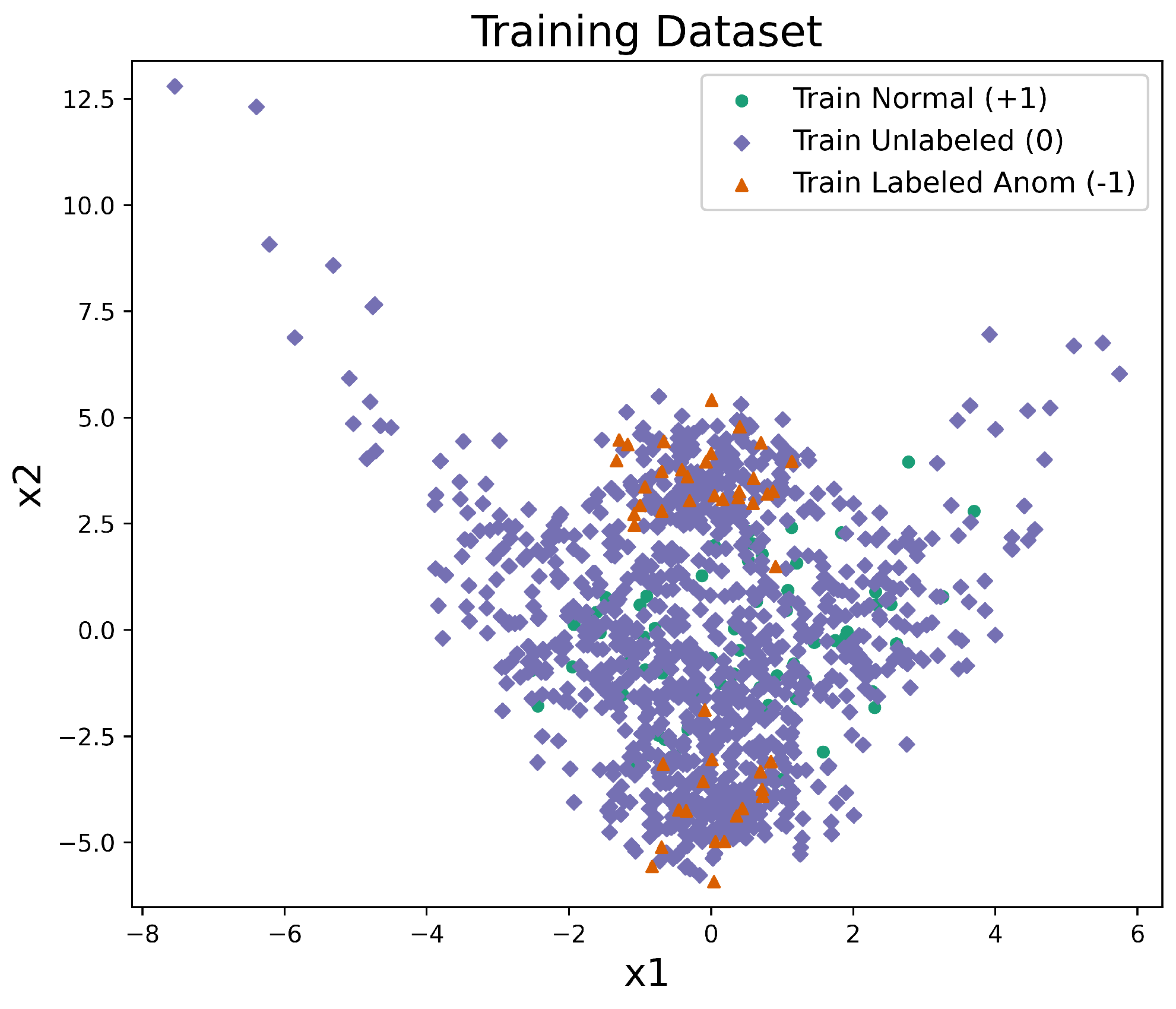
Figure 2.
Anomaly-score surfaces and decision boundaries on the synthetic banana dataset. The heat map shows the anomaly score , and the white dashed curve marks the selected decision boundary for each method. Panels (a) OC-SVM, (b) SVDD-RBF, (c) DeepSVDD, (d) DeepSAD, (e) AAG-DSVDD.
Figure 2.
Anomaly-score surfaces and decision boundaries on the synthetic banana dataset. The heat map shows the anomaly score , and the white dashed curve marks the selected decision boundary for each method. Panels (a) OC-SVM, (b) SVDD-RBF, (c) DeepSVDD, (d) DeepSAD, (e) AAG-DSVDD.
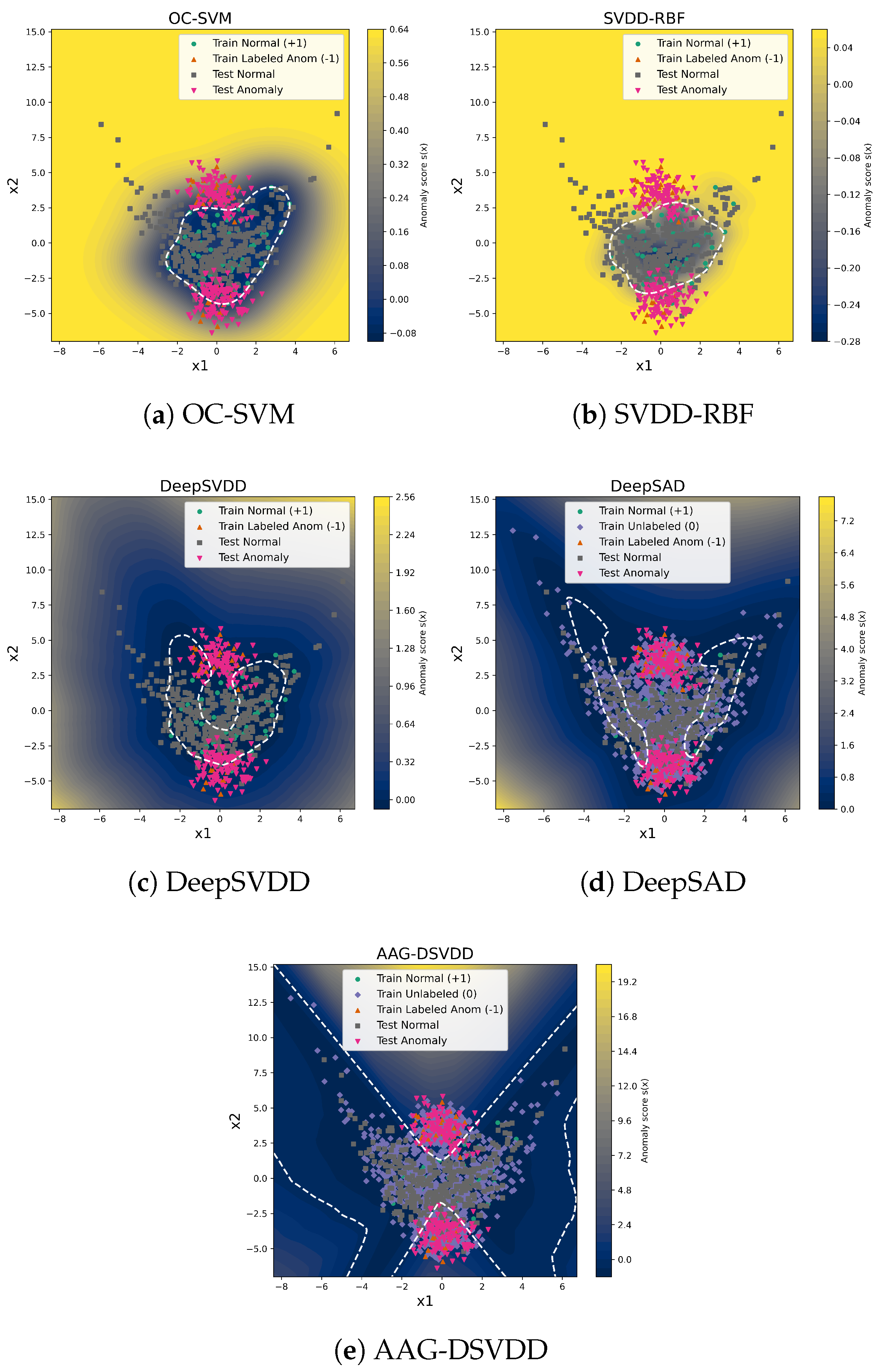
Figure 3.
Effect of the graph regularization weight on F1-score and precision for AAG-DSVDD on the synthetic banana dataset. Performance is stable for small to moderate and degrades for very strong regularization.
Figure 3.
Effect of the graph regularization weight on F1-score and precision for AAG-DSVDD on the synthetic banana dataset. Performance is stable for small to moderate and degrades for very strong regularization.
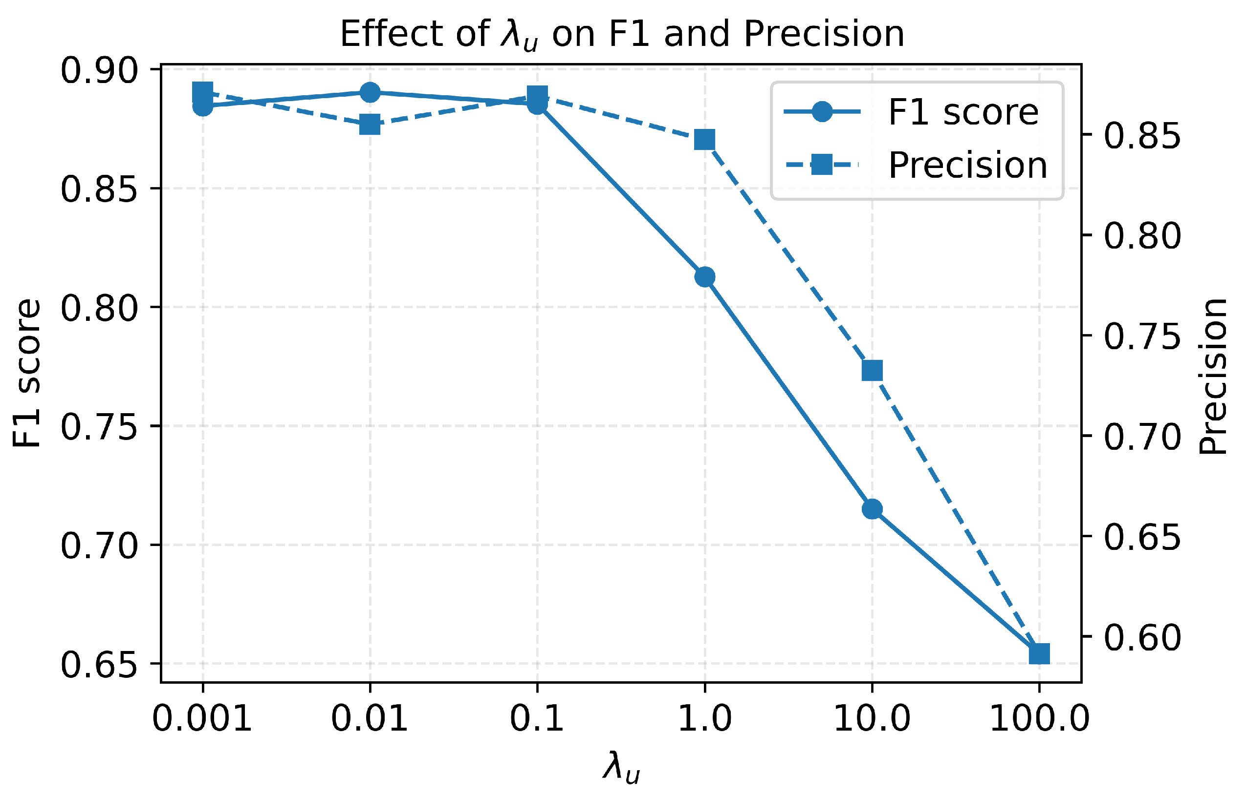
Figure 4.
Example multi-sensor signals from a flaming-fire scenario. Each panel shows one sensor channel sampled at 1 Hz: temperature (top), CO concentration, ionization smoke, photoelectric smoke, and smoke obscuration (bottom). The vertical dotted line marks the annotated TFST.
Figure 4.
Example multi-sensor signals from a flaming-fire scenario. Each panel shows one sensor channel sampled at 1 Hz: temperature (top), CO concentration, ionization smoke, photoelectric smoke, and smoke obscuration (bottom). The vertical dotted line marks the annotated TFST.
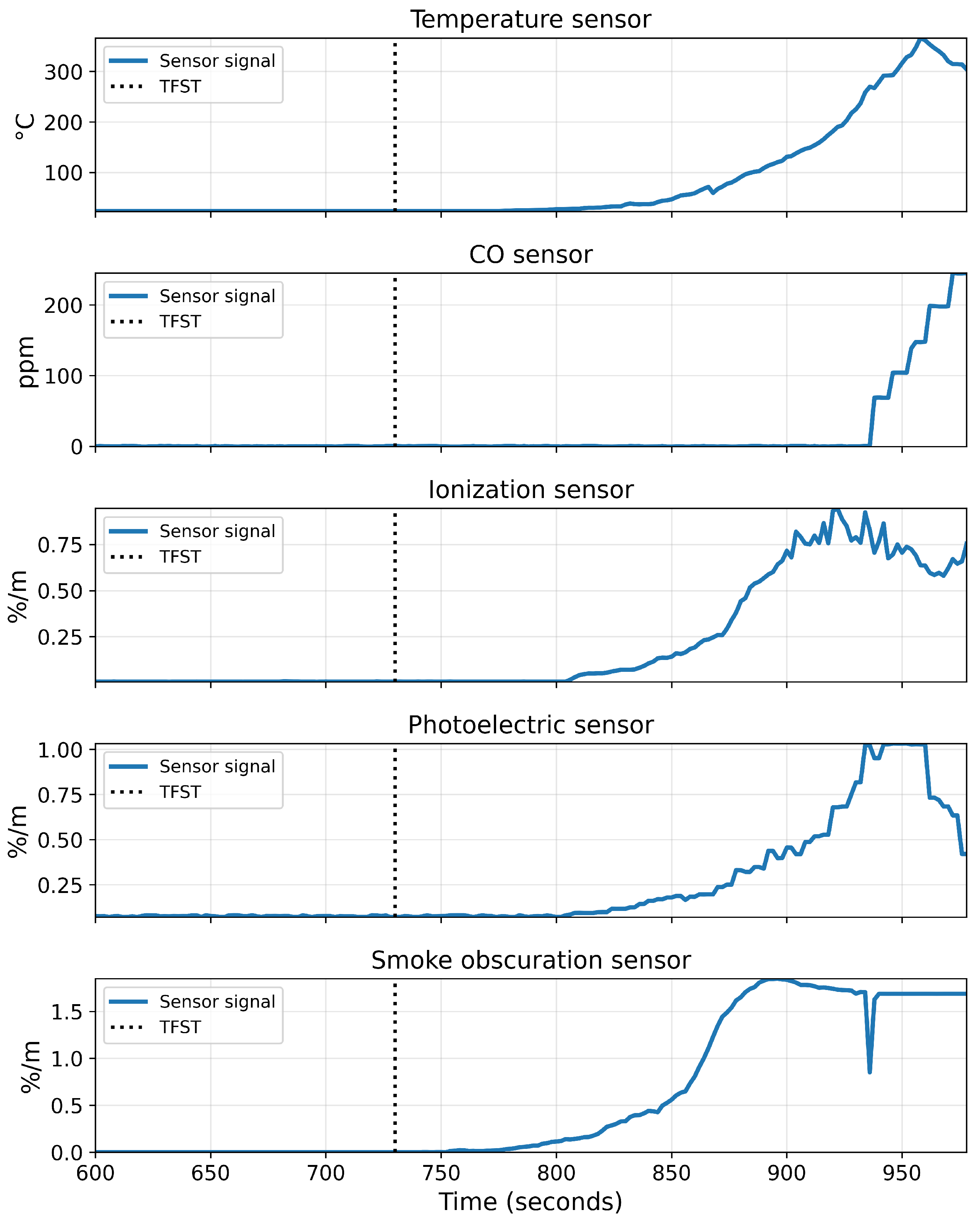

Table 1.
Comparison of anomaly detection methods’ performance on the synthetic banana dataset.
| Model | F1 | Recall | Precision | Accuracy |
|---|---|---|---|---|
| OC-SVM | 0.6625 | 0.6667 | 0.6584 | 0.7283 |
| SVDD-RBF | 0.7259 | 0.8167 | 0.6533 | 0.7533 |
| DeepSVDD | 0.6055 | 0.6875 | 0.5410 | 0.6417 |
| DeepSAD | 0.6510 | 0.9792 | 0.4876 | 0.5800 |
| AAG-DSVDD | 0.8852 | 0.9000 | 0.8710 | 0.9067 |
Table 2.
F1 performance on the synthetic banana dataset over 10 random seeds. The row “Mean ± Std” reports the average and standard deviation over seeds. The last two rows give one-sided paired t-test and Wilcoxon signed-rank p-values for the null hypothesis that each baseline has F1 at least as large as AAG-DSVDD.
| Seed | OC-SVM | SVDD-RBF | DeepSVDD | DeepSAD | AAG-DSVDD |
|---|---|---|---|---|---|
| 0 | 0.66 | 0.73 | 0.61 | 0.65 | 0.89 |
| 1 | 0.83 | 0.83 | 0.66 | 0.68 | 0.88 |
| 2 | 0.65 | 0.75 | 0.51 | 0.63 | 0.90 |
| 3 | 0.79 | 0.70 | 0.66 | 0.64 | 0.89 |
| 4 | 0.62 | 0.78 | 0.57 | 0.65 | 0.88 |
| 5 | 0.75 | 0.74 | 0.68 | 0.64 | 0.86 |
| 6 | 0.78 | 0.82 | 0.67 | 0.65 | 0.88 |
| 7 | 0.74 | 0.76 | 0.72 | 0.64 | 0.88 |
| 8 | 0.63 | 0.79 | 0.58 | 0.68 | 0.88 |
| 9 | 0.68 | 0.76 | 0.58 | 0.63 | 0.84 |
| Mean ± Std | |||||
| – | |||||
| – |
Table 3.
Fire scenarios used for training and testing in the AAG-DSVDD fire monitoring case study.
| Scenario ID | Split | Fire Type | Scenario Length (s) | TFST (s) |
|---|---|---|---|---|
| 1 | Train | Smoldering | 9104 | 1000 |
| 2 | Train | Heating | 2382 | 854 |
| 3 | Train | Flaming | 1024 | 652 |
| 4 | Train | Flaming | 948 | 730 |
| 5 | Test | Smoldering | 4455 | 968 |
| 6 | Test | Heating | 2642 | 1001 |
| 7 | Test | Flaming | 1210 | 1001 |
| 8 | Test | Flaming | 1186 | 1001 |
| 9 | Test | Flaming | 1192 | 1001 |
| 10 | Test | Flaming | 975 | 739 |
1 Scenario Length is the duration of the scenario in seconds. TFST is the true fire starting time in seconds.
Table 4.
Per-scenario fire detection performance on the test scenarios.
| Scenario # |
Scenario length |
TFST | OC-SVM | SVDD-RBF | DeepSVDD | ||||||
|---|---|---|---|---|---|---|---|---|---|---|---|
| EFST | FSTA | FAR | EFST | FSTA | FAR | EFST | FSTA | FAR | |||
| 5 | 4455 | 968 | 308 | 660 | 13.9 | 4455 | 3487 | 0.0 | 5 | 963 | 37.0 |
| 6 | 2642 | 1001 | 753 | 248 | 6.2 | 2642 | 1641 | 0.0 | 5 | 996 | 96.1 |
| 7 | 1210 | 1001 | 1110 | 109 | 0.0 | 1210 | 209 | 0.0 | 1046 | 45 | 0.0 |
| 8 | 1186 | 1001 | 1082 | 81 | 0.0 | 1186 | 185 | 0.0 | 699 | 302 | 2.0 |
| 9 | 1192 | 1001 | 1085 | 84 | 0.0 | 1192 | 191 | 0.0 | 1056 | 55 | 0.2 |
| 10 | 975 | 739 | 849 | 110 | 0.0 | 975 | 236 | 0.0 | 777 | 38 | 0.0 |
| Average | 864.5 | 215.3 | 3.4 | 1943.3 | 991.5 | 0.0 | 598.0 | 399.8 | 22.6 | ||
|
Scenario # |
Scenario length |
TFST | DeepSAD | AAG-DSVDD | |||||||
| EFST | FSTA | FAR | EFST | FSTA | FAR | ||||||
| 5 | 4455 | 968 | 4287 | 3319 | 0.0 | 2067 | 1099 | 0.0 | |||
| 6 | 2642 | 1001 | 738 | 263 | 1.7 | 2288 | 1287 | 0.0 | |||
| 7 | 1210 | 1001 | 1171 | 170 | 0.0 | 1164 | 163 | 0.0 | |||
| 8 | 1186 | 1001 | 1120 | 119 | 0.0 | 1125 | 124 | 2.5 | |||
| 9 | 1192 | 1001 | 1161 | 160 | 0.0 | 1129 | 128 | 1.6 | |||
| 10 | 975 | 739 | 839 | 100 | 0.0 | 776 | 37 | 0.0 | |||
| Average | 1552.7 | 688.5 | 0.3 | 1424.8 | 473.0 | 0.7 | |||||
Averages are computed over the six test scenarios. FSTA is reported in seconds and equals at 1 Hz sampling. FAR is the percentage of pre-TFST windows predicted as fire.
Disclaimer/Publisher’s Note: The statements, opinions and data contained in all publications are solely those of the individual author(s) and contributor(s) and not of MDPI and/or the editor(s). MDPI and/or the editor(s) disclaim responsibility for any injury to people or property resulting from any ideas, methods, instructions or products referred to in the content. |
© 2025 by the authors. Licensee MDPI, Basel, Switzerland. This article is an open access article distributed under the terms and conditions of the Creative Commons Attribution (CC BY) license (http://creativecommons.org/licenses/by/4.0/).
Copyright: This open access article is published under a Creative Commons CC BY 4.0 license, which permit the free download, distribution, and reuse, provided that the author and preprint are cited in any reuse.


