
Submitted:
20 October 2025
Posted:
22 October 2025
You are already at the latest version
Abstract
This paper presents a graph-attention-regularized deep anomaly detection framework for semi-supervised settings where normal labeled data is scarce and unlabeled data is abundant and contaminated (i.e., includes normal and anomaly points). Unlike conventional one-class and graph-based semi-supervised anomaly detection approaches, which either ignore unlabeled structure or do not utilize the structure effectively through data density breaks, the proposed method constructs an attention-weighted latent k-NN graph to capture unlabeled geometry while reducing the influence of contaminated neighbors. We formulate a new deep support vector data description variant, graph-attention-regularized deep support vector data description, that embeds this attention-weighted graph directly into the one-class objective incorporated with a center-pull regularization for unlabeled data to avoid decision boundary over smoothness, thereby effectively leveraging unlabeled data geometry and information. Experiments on simulated and an industrial windshield-wiper acoustics datasets validate the effectiveness of the proposed approach under scarce-label conditions relative to existing deep and shallow methods.
Keywords:
acoustic anomaly detection
; attention-weighted graphs
; automotive quality control
; GAR-DSVDD
; semi-supervised anomaly detection
; SVDD
; windshield-wiper fault detection
MSC: 68T05; 68T07; 62H30
1. Introduction
Anomaly detection is a critical issue in machine
learning, with applications in manufacturing, industrial process control,
medical diagnosis, cybersecurity, and disaster management [1,2,3,4,5]. The primary objective is to learn a
representation of normal operating conditions and identify deviations as
anomalies. Unlike standard supervised classification, anomaly detection is
characterized by severe class imbalance, where anomalies are rare, diverse, and
often scarcely labeled, while normal samples are abundant. However, despite
this abundance, labeling a sample as truly normal is often costly and
challenging. In many operational settings, normal labeling requires expert
review against process specifications, additional quality-control checks
(sometimes destructive or time-consuming), or prolonged observation to rule out
hidden faults. These steps consume engineer time and test resources and can
cause production downtime, making exhaustive normal labeling economically
impractical at scale. For instance, in automotive quality management, current
practice for windshield-wiper noise relies on expert assessment: after
controlled recordings, mel
frequency cepstral coefficients/spectrogram features are computed,
and an expert labels the noise types [6].
Early efforts in one-class classification
introduced support vector data description (SVDD) and the one-class support
vector machine (OC-SVM) as core frameworks. SVDD learns a minimum-radius
hypersphere that encloses the normal training data, predicting observations
outside the decision boundary as anomalies [7].
The OC-SVM learns a maximum-margin separator from the origin in feature space
to capture the support of the normal distribution [8].
While these models produce compact, interpretable decision boundaries, they
generally require a clean set of normal samples and do not utilize unlabeled
data, thereby limiting their effectiveness when normal labeling is costly and
unlabeled observations are abundant.
Graph-based semi-supervised learning offers a
systematic approach to utilize unlabeled data by representing adjacency and
manifold structure. The basic concepts of spectral graphs and Laplacian
regularization define the cluster assumption through the concept of smoothness
across neighborhoods [9,10]. Recent studies
and applications in graph anomaly detection indicate extensive utilization
across nodes, edges, subgraphs, and whole graphs [11,12,13].
SVDD has been extended using semi-supervised methods that utilize the structure
of unlabeled data while employing a small number of labeled normal observations
to guide the boundary. In order to leverage large unlabeled data without hard
pseudo-labels, a common practice is to enhance the SVDD objective with
manifold/graph regularization so that points connected on a similarity graph
remain close in the learned representation [9,10].
One SVDD variant, graph-based semi-supervised SVDD (S3SVDD), leverages
global/local geometric structure with limited labels by utilizing a -nearest neighbor (-NN) spectral graph and a Laplacian smoothness term
in the SVDD objective to exploit unlabeled data [14].
Similarly, semi-supervised subclass SVDD proposes a new formulation that
utilizes global/local geometric structure with limited labels [15]. Separately, a manifold-regularized SVDD for
noisy label detection was introduced, showing that incorporating a graph
Laplacian into the SVDD objective improves robustness to label noise while
still leveraging abundant unlabeled data [16].
In addition, a semi-supervised convolutional neural network (CNN) with SVDD has
demonstrated practical viability in industrial monitoring [17]. While traditional graph-based SVDD variants
have shown potential, these methods typically rely on fixed, pseudo-labeled
neighbor graphs (e.g., -NN with a chosen metric and ) and uniform edge weights, which can over-connect
across data density breaks, propagate contamination from suspect (anomalous)
neighbors, and require careful tuning [9,14,18,19,20].
The introduction of deep learning has led to
significant advances in deep anomaly detection. Deep SVDD (DeepSVDD) extended
the SVDD framework by combining it with a deep encoder that maps data into a
latent representation enclosed by a hypersphere [21].
Autoencoders and their variants have been widely adopted to learn
low-dimensional embeddings and reconstruction-based anomaly scores in
industrial and time-series contexts [22,23].
Additionally, self-supervised anomaly detection has emerged as a promising
direction by utilizing contrastive learning and related pretext objectives that
enhance representation quality under limited labels [24,25].
However, common deep anomaly detection methods often use objectives that are
indirectly aligned with the decision boundary (e.g., reconstruction error),
leverage unlabeled data using proxy tasks rather than task-aware constraints in
the decision boundary learner, and offer limited interpretability of decisions [26,27,28,29,30,31].
Motivated by the aforementioned challenges, this
paper presents Graph-Attention-Regularized Deep SVDD (GAR-DSVDD). Specifically,
we develop a semi-supervised Deep SVDD that trains a deep encoder and a
one-class hypersphere end-to-end, while exploiting unlabeled structures with a
center-pull regularizer on a learned graph. To build this graph, we introduce
an attention-weighted latent -NN mechanism that assigns label and score-aware
importance to neighbors, emphasizing prototypical normal observations and
down-weighting suspect or anomalous samples, thereby mitigating label scarcity
and limiting error propagation from contaminated edges. Unlike iterative
pseudo-labeling methods, our training uses unlabeled data directly through the
center-pull and graph smoothness regularizers, which stabilize optimization and
reduce computation. For safety-critical deployment, per-instance attention weights
provide transparent explanations over the top- neighbors. Comprehensive experiments on a
simulated dataset and an industrial windshield-wiper acoustics case study show
that GAR-DSVDD achieves superior detection of subtle anomalies compared with
classical and deep learning benchmarks, while reducing labeling effort and
operator subjectivity.
The remainder of the paper is structured as
follows. Section 2 reviews preliminaries
and notation for semi-supervised anomaly detection. Section 3 presents the proposed GAR-DSVDD
method. Section 4 describes the
experimental setup and reports results on simulated datasets and the
windshield-wiper acoustics case study, along with sensitivity analyses. Section 5 discusses findings, conclusions, and
potential future work directions.
2. Preliminaries
2.1. Data and Basic Notation
Given a training dataset that decomposes into two disjoint subsets: a small
set of labeled normal samples and a large unlabeled set , with
Let be the index set of labeled normal observations
and the unlabeled indices, with , , and label rate . The unlabeled pool is assumed predominantly
normal and may contain a small contamination of anomalies, upper-bounded by . Features are standardized by coordinate
(z-scoring). A learnable encoder maps each input to a latent representation, where denotes the encoder’s trainable parameters; we
write and collect latents as . We stack them row-wise in . We use for the Euclidean norm and for the standard inner product in . This setting follows the deep one-class paradigm:
the normal class is to be enclosed within a compact latent region while
avoiding pseudo-labels for the unlabeled pool. Instead, informs the latent geometry via a graph defined
over (details in §3).
2.2. Latent One-Class Score
We summarize the normal set by a latent center and a soft margin (squared radius) used for score
calibration
Given latents with , the per-sample anomaly score is
A sample is more anomalous
as increases; the decision boundary is . Eq. (1) gives the deep “hypersphere” view of SVDD
in latent space, where summarizes the normal set and maps inputs to latents. The offset specifies the boundary tolerance (squared radius)
via a softplus parameterization, ensuring positivity and smooth gradients near
the boundary. The center is typically initialized as the mean of to stabilize early training. The score is
scale-aware: increasing relaxes the boundary, whereas decreasing tightens the enclosure, preserving the
boundary-level interpretation (distance to versus tolerance ). During training, is treated as a calibration constant, so choosing
a train-quantile threshold on f
is equivalent to thresholding the same quantile of .
3. Graph-Attention-Regularized Deep SVDD
We now detail GAR-DSVDD. The objective has three
parts: (i) a one-class enclosure on labeled normal observations, (ii) an
unlabeled neighbor-smoothness on squared distances over an attention-weighted
directed, row-normalized -NN graph, and (iii) standard parameter
regularization.
3.1. Latent Attention-Weighted -NN Graph
We construct a directed row-normalized graph over the latent set , where each latent is produced by the encoder , and we stack them row-wise as . For each node , define the directed neighborhood as the indices of the -NN of under a base metric (Euclidean by default). Each
candidate edge carries a base affinity , chosen as either a Gaussian kernel or a constant:
To emphasize true normal observations and suppress
suspect connections (possible anomalies), we compute score-aware attention on
each edge. With heads, the per-head logits are
where are linear projections (shared across pairs for
head ), is the attention width, is a contamination reducing coefficient, and is the current one-class score (Eq. (1)). We
normalize within using a temperature -scaled softmax:
and aggregate heads by averaging
We integrate attention with the base affinity using
and then row-normalize the outgoing weights:
Edges outside have weight ( if ). Row-normalization preserves scale across
heterogeneous densities (outgoing weights sum to 1) and reduces error
propagation by down-weighting high-score (potentially anomalous) edges during
training. We compute attention weights without back-propagation and keep them
fixed between graph refreshes. Prior work motivating the attention graphs to
interpret unlabeled data geometry includes [9,10,32].
To keep training tractable, we do not materialize a
full graph at every step. Instead, we rebuild a latent-space -NN index periodically and, for each mini-batch,
form edges as the union of (i) cached neighbors of the batch points and (ii)
within-batch -NN edges—preserving local geometry for the
smoother while keeping computation practical.
3.2. Unlabeled Geometry via Neighbor-Smoothness on Squared Distances
Let
Unlabeled samples help create a smooth decision
boundary by discouraging sharp variations of along high weight edges of the attention-weighted
graph (described in §3.1):
Penalizing differences of (rather than feature vectors) aligns the boundary
with high-density regions without collapsing representations and preserves the
simple one-class test rule on .
The derivatives of are
and by the chain rule
so
and
During training, we rebuild the graph periodically
and hold fixed within each interval, so we do not
back-propagate through the weights in this term.
3.3. Labeled-Normal Enclosure
Labeled normal observations anchor the hypersphere in latent space through a
distance-based objective:
where , is a latent center summarizing the normal set. and
weakly centers the hypersphere. This formulation
directly penalizes the squared distance of labeled normal observations from yielding stable gradients and a simple coupling to
the encoder.
The gradients of are
Since , by the chain rule
3.4. Unlabeled Center-Pull
To stabilize training when the labeled normal set is small, we add a label-free pull of the
unlabeled latents toward the center . This acts on raw squared distances and complements the neighbor smoothness. The graph
term equalizes differences of along edges and is largely insensitive to the
global level of ; with few labelled observations this can cause
scale drift and a poorly calibrated score . Moreover, early graphs may include contaminated
edges (unlabeled anomalies can appear inside or near the hypersphere), so
smoothing alone can propagate their influence. The center-pull softly anchors
the mean of for the normal unlabeled pool, reducing drift and
reducing contamination while the graph term aligns local variations.
We define
This imposes a global constraint by shrinking the
mean of over toward . Unlike —which is local and relative— fixes the overall scale and prevents drift when
labels are scarce, improving calibration of .
The gradients are
Since , by the chain rule
3.5. GAR-DSVDD Objective Function
The total loss combines unlabeled geometry, labeled-normal
enclosure, and unlabeled center pull:
with , , and as in Eqs. (3), (4), and (5), respectively, the
scalars control the strengths of the graph regularizer and
unlabeled center pull.
Together, , , and play complementary roles: anchors the center using trusted labeled normals, preventing center
drift; enforces local consistency of squared distances on
the attention-weighted, row-normalized -NN graph, transferring structure from the
unlabeled pool without collapsing features; and imposes a global moment constraint on unlabeled
data, fixing the overall scale of and improving calibration of the score .
We train jointly using the AdamW optimizer. The
attention-weighted -NN graph is recomputed every epochs and held fixed within those intervals. No
gradients flow through the attention computation or through . At deployment, a testing observation can be labeled as an anomaly if its score exceeds a train-quantile threshold otherwise it will be considered as normal.
In summary, GAR-DSVDD combines a deep one-class
boundary with graph-based semi-supervision in a way that is both robust and
label-efficient. By regularizing squared distance (scores)—not features—over an
attention-weighted latent -NN graph, it aligns the decision boundary with the
data manifold without collapsing representations and preserves the simple
test-time rule . Score-aware attention selectively down-weights
suspicious neighbors, curbing over-smoothing from contaminated edges and
density breaks. In addition to this, local, edge-wise smoothing of , an unlabeled center-pull imposes a global moment
constraint that stabilizes the overall scale of the distance field, improving
score calibration when labeled normal observations are scarce. Because
unlabeled data enter only through these geometric regularizers (no
pseudo-labels), a small labeled set is enough to anchor the hypersphere while
the unlabeled pool shapes the boundary. Thus, the proposed method effectively
utilizes information from labeled and unlabeled observations for enhanced
anomaly detection in semi-supervised settings.
| Algorithm: GAR-DSVDD (training) |
| Inputs: , ; ; graph params ; weights ; refresh period T ; total epochs . |
Outputs: decision threshold .
|
|
Inference (testing) Given xnew:
|
(Note: is the attention softmax temperature; is the decision threshold).
4. Experiments
In order to evaluate the performance of the
proposed method, we apply it to a semi-supervised setting over a simulated
dataset to visualize behavior and an industrial case study in the domain of
industrial automotive quality management, where windshield wiper reversal noise
is detected.
4.1. Experimental Setup
Experiments are conducted on a simulated two-dimensional
dataset and a real industrial windshield-wiper acoustics dataset to
compare the proposed GAR-DSVDD against established methods, including DeepSVDD, OCSVM, classical SVDD, and S3SVDD. All deep models share the same encoder
capacity and optimization schedule for fairness. Threshold calibration follows
each method’s policy: for GAR-DSVDD and DeepSVDD, we use a train-quantile rule
at a fixed level over labeled-normal scores, whereas OCSVM, SVDD, and S3SVDD
use their native decision functions. Across both experiments, training follows
a semi-supervised setting: a small subset of labeled normal samples and a large
unlabeled pool that may include a small contamination of anomalies (bounded by ). We construct four disjoint partitions: labeled normal
observations, unlabeled, validation, and a held-out test set.
Performance is evaluated on the held-out test split
using four measures derived from the confusion counts—true positives (TP),
false positives (FP), true negatives (TN), and false negatives (FN).
Overall accuracy (fraction of correctly classified
instances):
Detection rate (also called recall or true positive
rate), measuring how many anomalies are correctly detected:
The F1 score summarizes the trade-off between
precision and detection rate under class imbalance. Define precision as
then
Balanced accuracy, averaging sensitivity (detection
rate) and specificity (true negative rate). First define specificity
then
For each dataset/seed, we test the directional
alternative : GAR-DSVDD >
benchmark on the F1 score using paired -tests and Wilcoxon signed-rank tests across seeds
and report their p-values.
4.2. Simulated Data
In the simulated study, we utilize a two-cluster,
two-dimensional dataset that has separable centers and evaluate it under a
semi-supervised setting. We draw normal observations and anomalies, label a small fraction of normal
observations , set unlabeled contamination to , and reserve for validation andfor testing. Figure
1 shows the training dataset used for the experiment, where labeled and
unlabeled observations are used to train GAR-DSVDD and S3SVDD, while the other
methods use labeled observations only. We carried out a total of 10
experiments, using different seeds when generating the data. The training set
for one of the experiments is illustrated in Figure
1.
All deep methods share the same encoder for fairness: a two-layer MLP with hidden widths mapping with ReLU activations. Our method constructs a
latent -NN graph on with and attention weights ( heads, key dimension ). The attention-weighted graph is recomputed every
epochs and held fixed between refreshes; no
gradients flow through the attention computation. We optimize the objective in
Eq. (6) using AdamW for epochs with refresh rate and learning rate , graph regularizer strength , and unlabeled center pull strength . Lastly, we calibrate by setting it to the same train-quantile used for
threshold selection over labeled normals.
As for the remaining methods, DeepSVDD is trained
on labeled normal using the same applicable parameters of the proposed method,
OSCVM uses , SVDD uses radial basis function (RBF) kernel
parameter , and S3SVDD uses RBF kernel parameter with = 9. The deep methods use a train-quantile rule at
, and the native decision function is used for the
rest.
The performance results of the proposed methods
compared to benchmarking methods over all testing performance metrics for an
experiment are shown in Table 1, whereas Table 2 compares their F1 score over 10
different testing sets where the data was generated using different seeds.
DeepSVDD trains only on labeled normal observations
and learns a tight hypersphere where many normal observations on low-density
areas fall outside it, thus, increasing false positive rate and reducing
overall accuracy, and F1 despite having high detection rate. OCSVM lacks
representation learning and geometry-aware regularization, thus constructing a
narrow decision boundary where detection rate remains high, but specificity and
overall accuracy suffer, leading to a lower F1 score. Since classical SVDD does
not utilize unlabeled-geometry guidance, it builds a decision boundary based on
labeled observation alone, thus, obtaining a tight hypersphere yielding to a
high false positive rate and reduced accuracy and F1 score. Incorporating a
fixed-weight graph S3SVDD shows similar performance to SVDD as fixed-weight
graph cannot truly suppress influence of suspect (anomalous) neighbors, thus,
assumes that most unlabeled observations are anomalous and constructs a narrow
hypersphere.
In contrast, the attention-weighted GAR-DSVDD
achieves the best F1 and balanced accuracy, among all other methods, by pairing
high detection and lower false positives. Attention down weights influence from
suspect neighbors in the unlabeled graph, limiting score dispersal from
contaminated (anomalous) points and keeping the boundary near density valleys.
The center pull regularizer on unlabeled observations prevents over smoothing
decision boundary, preserving overall accuracy, while labeled normal observations
ensure that the hypersphere is anchored to the normal region. Overall,
GAR-DSVDD yields a more robust hypersphere across all experiments.
The obtained anomaly score and its quantiles are
shown in Figure 2. In the figure, the quantile contour for the anomaly score is drawn to
indicate the decision boundary for the deep methods, where the native decision
boundary is shown for the shallow methods. Note that DeepSVDD and GAR-DSVDD use
a single hypersphere in latent space as its decision region based on the
learned quantile. In the figure, after the encoder’s nonlinear mapping back to
input space, this can look complex or even disconnected, despite being one
sphere in the learned latent space.
4.3. Case Study: Windshield-Wiper Acoustics
This section presents our case study on windshield
wiper acoustics. We analyzed windshield-wiper sound recordings gathered under
tightly controlled laboratory conditions. Each sample was captured from
production wiper assemblies inside an anechoic chamber while a sprinkler system
supplied water to replicate rainfall. To eliminate confounding noise sources,
the vehicle’s engine remained off, and the wiper motor was powered by an
external supply. A fixed in-cabin microphone recorded the acoustic pressure signal,
which was calibrated and expressed in decibels at a constant sampling rate.
Domain specialists reviewed the recordings and assigned ground-truth labels
covering reversal noise fault phenomena alongside normal operation. The dataset
consists of a total of 120 windshield wiper recordings, where 61 recordings are
for normal operations and 59 for faulty (anomalous) operations. These expert
annotations are treated as ground truth for evaluation.
Each observation is a single full recording
summarized as a fixed-length vector from recording descriptors, in line with
recent acoustic research for sound analysis. We compute 32 MFCCs to capture the
spectral envelope on a perceptual scale, together with first- and second-order
deltas to encode short-term dynamics; these cepstral families remain standard
and effective in contemporary studies. We also include a 12-bin chroma profile
to reflect tonal/resonant structure and simple spectral/temporal statistics—spectral
centroid, spectral bandwidth, spectral roll-off at 95%, root-mean-square (RMS)
energy, and zero-crossing rate (ZCR)—which are routinely used and compared in
modern journal work. For every multi-frame descriptor with coefficients, we pool across time by concatenating
the per-coefficient mean and standard deviation, so each such descriptor
contributes values; scalar descriptors contribute two values
(mean and standard deviation). Summing up all parts yields a dimensional vector per recording of means and
standard deviations across time that we use for the reversal-noise dataset.
These choices (MFCCs with deltas, chroma, and spectral statistics with mean/std
pooling) align with recent papers documenting their efficacy and definitions
across environmental-sound, speech-emotion, smart-audio, and urban-acoustic
applications [33,34,35]. Figure 3 shows normal and anomaly operation
recordings of windshield wipers with their corresponding MFCC features on the
log scale. Table 3 summarizes the feature
extraction methods used for acoustic analysis of the windshield wiper sound
recordings.
We follow the same semi-supervised protocol as in the simulated study: a small subset of labeled-normal clips is provided, and a large unlabeled pool may include mild anomaly contamination; the remainder is split into validation (for hyperparameter selection) and a held-out test set. Concretely, we use a 60/20/20 split for train/validation/test. Within the training portion, we label 10% of the normal observations () and place the rest into the unlabeled set with anomaly contamination ratio . All deep methods use the shared encoder : a two-layer MLP with ReLU activations. For our method, GAR-DSVDD, we build a latent -NN graph with and multi-head attention (8 heads, key dimension 32) over the encoder representations. The attention-weighted graph is recomputed every epochs and held fixed between refreshes; no gradients flow through the attention computation. The objective in Eq. (6) for 120 epochs using AdamW (learning rate ), graph regularizer strength , and unlabeled center pull strength . is calibrated by setting it to the same train-quantile used for threshold selection over labeled normals.
Benchmarks are configured to match their best settings from the wiper runs: DeepSVDD is trained on labeled normal observations with the same encoder/optimizer, soft-boundary objective regularizer value ; OCSVM uses with an RBF kernel ; SVDD uses an RBF kernel with ; and S3SVDD employs a NN graph with and RBF . The deep methods apply a train-quantile rule with , while OCSVM, SVDD, and S3SVDD use their native decision function.
The performance of GAR-DSVDD and the existing methods overall performance metrics are presented in Table 4. Table 5 shows the F1 score over 10 different testing sets that were prepared using 10 different seeds for statistical validation.
Due to the extreme challenges represented by this dataset and the semi-supervised experiment settings with very few training labeled normal observation, all benchmarking methods perform poorly for anomaly detecting as they fail to utilize unlabeled observations in constructing their decision boundaries as indicated by the F1 and accuracy metrics. The decision boundary obtained by these methods tend to be very narrow, causing most testing observations to be detected as anomalies while increasing the false positive rates, as seen by the specificity metric for these methods.
In contrast, GAR-DSVDD maintains perfect detection while achieving a higher specificity by leveraging an attention-weighted latent -NN graph that weakens edges in mixed or uncertain neighborhoods, thus, effectively utilizing information from unlabeled observation. This reduces the graph-driven propagation of elevated scores into nearby normal observations, keeps the decision boundary aligned with low-density regions, and prevents the false positive rates that undermine the other methods. Furthermore, the learned neighbor attention weights serve as per-instance attributes, indicating which historical normal observations most influence a observation’s score. In an industrial setting, these attributions can streamline expert review and reduce the volume of fully verified normal labels required over time, aligning the method with label-efficiency needs in automotive quality control.
4.4. Sensitivity Analysis
In this section, we perform sensitivity analysis over the simulated data. In Table 6 and Figure 4 we show the effect of increasing the normal labeled observations ratio over the F1 performance of the methods. Across labeled-normal ratios , the results show a clear label-efficiency advantage for our semi-supervised GAR-DSVDD in the low-label setting, with supervised baselines gradually converging as ρ increases. With scarce labels, GAR-DSVDD leads, consistent with its attention-weighted graph regularization that leverages unlabeled structure while mitigating contamination. As the label budget grows to a moderate level, GAR-DSVDD remains best, but the gap narrows, particularly with DeepSVDD, which benefits directly from richer labeled evidence. OCSVM improves steadily with more labels yet trails the deep methods, while classical SVDD consistently lags despite incremental gains. S3SVDD exhibits non-monotonic behavior, sensitive to label density and split composition, but becomes more competitive with increased labeling ratio. In summary, when only a small portion of data can be labeled, our target operating point, GAR-DSVDD outperforms all alternatives; as labeling increases, purely supervised approaches like DeepSVDD catch up and have similar performance, whereas OCSVM and SVDD continue to benefit but remain behind, and S3SVDD’s competitiveness depends on the labeling setting.
Moreover, by setting , we analyze the effect of on F1 and accuracy of GAR-DSVDD, as illustrated in Figure 5. For small , less importance is given to unlabeled geometry, thus, the unlabeled information is underutilized, leading to narrow decision boundary and underperforming results. Increasing gives more importance to the graph-loss term (unlabeled geometry), which expands the decision boundary with consistent gains in performance. The performance is highest near 1300, where the boundary best balances the influence of labeled data information, unlabeled geometry, and central-pull term on unlabeled observations. At higher values, excessive emphasis on unlabeled geometry over-smooths the graph structure, widening the decision boundary and allowing anomalous unlabeled observations to be included within the decision boundary, thereby degrading performance. These findings indicate that should be carefully selected via validation to allow an optimal construction of the decision boundary that keeps anomalous unlabeled observations outside and expands enough to keep normal behavior observations inside.
5. Conclusions
Identifying anomalies is a critical issue in applications such as manufacturing, industrial process control, cybersecurity, disaster management, and medical diagnosis, as they provide information about deviations from normal behaviour in critical environments [1,2,3,4,5]. Among available approaches, SVDD-based procedures remain attractive for their compact decision boundaries and test-time simplicity.
In this paper, we presented a GAR-DSVDD for semi-supervised anomaly detection. The method encloses labeled normal observations with a deep one-class boundary while propagating score-level smoothness over an attention-weighted latent -NN graph to leverage abundant unlabeled data. The attention mechanism reduces over-smoothing from questionable neighbors and respects local density breaks, improving specificity without sacrificing detection. Experiments on simulated data and a windshield-wiper acoustics case study demonstrate that GAR-DSVDD outperforms classical and deep baselines under scarce labels significantly.
Considering future work, many industrial datasets contain multiple normal classes (e.g., distinct operating conditions or product variants). Our current formulation targets a single normal class; extending it to multi-normal settings is a natural next step. One direction is to learn several hyperspheres using a shared encoder, where each hypersphere retains its corresponding normal class while discouraging overlapping with others; the graph attention can be made class-aware to limit cross-class leakage. Finally, online updates with periodic graph refresh and automatic selection of graph/attention hyperparameters would enhance robustness in evolving production environments.
Data Availability Statement
The industrial windshield wiper acoustic data presented in this study are available on reasonable requests from the corresponding author due to confidentiality. The code for the simulated dataset can be found at https://github.com/alhinditaha/GAR-DSVDD.
Acknowledgments
The project was funded by KAU Endowment (WAQF) at King Abdulaziz University, Jeddah, Saudi Arabia. The authors, therefore, acknowledge with thanks WAQF and the Deanship of Scientific Research (DSR) for technical and financial support.
Conflicts of Interest
The authors declare no conflicts of interest.
GenAI Usage Disclosure
No generative artificial intelligence (GenAI) technology was used for generating text, data or graphics, study design, or data collection, analysis or interpretation. GenAI tools (ChatGPT, OpenAI: GPT5) were solely used, under the authors’ supervision, to enhance readability and refine language (grammar, spelling, punctuation, and formatting). The paper has been carefully reviewed by the authors to ensure its accuracy and coherence.
Abbreviations
The following abbreviations are used in this manuscript:
| AdamW | Adaptive Moment Estimation with (decoupled) Weight decay |
| DeepSVDD | Deep Support Vector Data Description |
| GAR-DSVDD | Graph-Attention-Regularized Deep Support Vector Data Description |
| -NN | k-Nearest Neighbors |
| MFCC | Mel-Frequency Cepstral Coefficients |
| OCSVM | One-Class Support Vector Machine |
| ReLU | Rectified Linear Unit |
| S3SVDD | Graph-based Semi-Supervised Support Vector Data Description |
| SVDD | Support Vector Data Description |
References
- Li, H.; Boulanger, P. A survey of heart anomaly detection using ambulatory Electrocardiogram (ECG). Sensors 2020, 20, 1461. [Google Scholar] [CrossRef]
- Alhindi, T.J.; Alturkistani, O.; Baek, J.; Jeong, M.K. Multi-class support vector data description with dynamic time warping kernel for monitoring fires in diverse non-fire environments. IEEE Sensors Journal 2025. [Google Scholar] [CrossRef]
- Sakong, W.; Kim, W. An adaptive policy-based anomaly object control system for enhanced cybersecurity. IEEE Access 2024, 12, 55281–55291. [Google Scholar] [CrossRef]
- Karsaz, A. A modified convolutional neural network architecture for diabetic retinopathy screening using SVDD. Applied Soft Computing 2022, 125, 109102. [Google Scholar] [CrossRef]
- Cai, L.; Yin, H.; Lin, J.; Zhou, H.; Zhao, D. A relevant variable selection and SVDD-based fault detection method for process monitoring. IEEE Transactions on Automation Science and Engineering 2022, 20, 2855–2865. [Google Scholar] [CrossRef]
- Alhindi, T.J.; Baek, J.; Jeong, Y.-S.; Jeong, M.K. Orthogonal binary singular value decomposition method for automated windshield wiper fault detection. International Journal of Production Research 2024, 62, 3383–3397. [Google Scholar] [CrossRef]
- Tax, D.M.; Duin, R.P. Support vector data description. Machine learning 2004, 54, 45–66. [Google Scholar] [CrossRef]
- Schölkopf, B.; Platt, J.C.; Shawe-Taylor, J.; Smola, A.J.; Williamson, R.C. Estimating the support of a high-dimensional distribution. Neural computation 2001, 13, 1443–1471. [Google Scholar] [CrossRef]
- Zhu, X.; Ghahramani, Z.; Lafferty, J.D. Semi-supervised learning using gaussian fields and harmonic functions. In Proceedings of the Proceedings of the 20th International Conference on Machine Learning (ICML-03); 2003; pp. 912–919. [Google Scholar]
- Belkin, M.; Niyogi, P.; Sindhwani, V. Manifold regularization: A geometric framework for learning from labeled and unlabeled examples. Journal of machine learning research 2006, 7. [Google Scholar]
- Luo, X.; Wu, J.; Yang, J.; Xue, S.; Peng, H.; Zhou, C.; Chen, H.; Li, Z.; Sheng, Q.Z. Deep graph level anomaly detection with contrastive learning. Scientific Reports 2022, 12, 19867. [Google Scholar] [CrossRef]
- Ma, X.; Wu, J.; Xue, S.; Yang, J.; Zhou, C.; Sheng, Q.Z.; Xiong, H.; Akoglu, L. A comprehensive survey on graph anomaly detection with deep learning. IEEE transactions on knowledge and data engineering 2021, 35, 12012–12038. [Google Scholar] [CrossRef]
- Qiao, H.; Tong, H.; An, B.; King, I.; Aggarwal, C.; Pang, G. Deep graph anomaly detection: A survey and new perspectives. IEEE Transactions on Knowledge and Data Engineering 2025. [Google Scholar] [CrossRef]
- Duong, P.; Nguyen, V.; Dinh, M.; Le, T.; Tran, D.; Ma, W. Graph-based semi-supervised support vector data description for novelty detection. In Proceedings of the 2015 International Joint Conference on Neural Networks (IJCNN); 2015; pp. 1–6. [Google Scholar]
- Mygdalis, V.; Iosifidis, A.; Tefas, A.; Pitas, I. Semi-supervised subclass support vector data description for image and video classification. Neurocomputing 2018, 278, 51–61. [Google Scholar] [CrossRef]
- Wu, X.; Liu, S.; Bai, Y. The manifold regularized SVDD for noisy label detection. Information Sciences 2023, 619, 235–248. [Google Scholar] [CrossRef]
- Peng, D.; Liu, C.; Desmet, W.; Gryllias, K. Semi-supervised CNN-based SVDD anomaly detection for condition monitoring of wind turbines. In Proceedings of the International Conference on Offshore Mechanics and Arctic Engineering; 2022; p. V001T001A019. [Google Scholar]
- Von Luxburg, U. A tutorial on spectral clustering. Statistics and computing 2007, 17, 395–416. [Google Scholar] [CrossRef]
- Zelnik-Manor, L.; Perona, P. Self-tuning spectral clustering. Advances in Neural Information Processing Systems 2004, 17. [Google Scholar]
- Song, Y.; Zhang, J.; Zhang, C. A survey of large-scale graph-based semi-supervised classification algorithms. International Journal of Cognitive Computing in Engineering 2022, 3, 188–198. [Google Scholar] [CrossRef]
- Ruff, L.; Vandermeulen, R.; Goernitz, N.; Deecke, L.; Siddiqui, S.A.; Binder, A.; Müller, E.; Kloft, M. Deep one-class classification. In Proceedings of the International Conference on Machine Learning; 2018; pp. 4393–4402. [Google Scholar]
- Pota, M.; De Pietro, G.; Esposito, M. Real-time anomaly detection on time series of industrial furnaces: A comparison of autoencoder architectures. Engineering Applications of Artificial Intelligence 2023, 124, 106597. [Google Scholar] [CrossRef]
- Neloy, A.A.; Turgeon, M. A comprehensive study of auto-encoders for anomaly detection: Efficiency and trade-offs. Machine Learning with Applications 2024, 17, 100572. [Google Scholar] [CrossRef]
- Tack, J.; Mo, S.; Jeong, J.; Shin, J. Csi: Novelty detection via contrastive learning on distributionally shifted instances. Advances in Neural Information Processing Systems 2020, 33, 11839–11852. [Google Scholar]
- Hojjati, H.; Ho, T.K.K.; Armanfard, N. Self-supervised anomaly detection in computer vision and beyond: A survey and outlook. Neural Networks 2024, 172, 106106. [Google Scholar] [CrossRef] [PubMed]
- Chalapathy, R.; Chawla, S. Deep learning for anomaly detection: A survey. arXiv 2019, arXiv:1901.03407. [Google Scholar] [CrossRef]
- Pang, G.; Shen, C.; Cao, L.; Hengel, A.V.D. Deep learning for anomaly detection: A review. ACM Computing Surveys (CSUR) 2021, 54, 1–38. [Google Scholar] [CrossRef]
- Ruff, L.; Kauffmann, J.R.; Vandermeulen, R.A.; Montavon, G.; Samek, W.; Kloft, M.; Dietterich, T.G.; Müller, K.-R. A unifying review of deep and shallow anomaly detection. Proceedings of the IEEE 2021, 109, 756–795. [Google Scholar] [CrossRef]
- Li, Z.; Zhu, Y.; Van Leeuwen, M. A survey on explainable anomaly detection. ACM Transactions on Knowledge Discovery from Data 2023, 18, 1–54. [Google Scholar] [CrossRef]
- Bouman, R.; Heskes, T. Autoencoders for Anomaly Detection are Unreliable. arXiv 2025, arXiv:2501.13864. [Google Scholar] [CrossRef]
- Kim, S.; Lee, S.Y.; Bu, F.; Kang, S.; Kim, K.; Yoo, J.; Shin, K. Rethinking reconstruction-based graph-level anomaly detection: limitations and a simple remedy. Advances in Neural Information Processing Systems 2024, 37, 95931–95962. [Google Scholar]
- Velickovic, P.; Cucurull, G.; Casanova, A.; Romero, A.; Lio, P.; Bengio, Y. Graph attention networks. Stat 2017, 1050, 10–48550. [Google Scholar]
- Bansal, A.; Garg, N.K. Environmental Sound Classification: A descriptive review of the literature. Intelligent Systems with Applications 2022, 16, 200115. [Google Scholar] [CrossRef]
- Madanian, S.; Chen, T.; Adeleye, O.; Templeton, J.M.; Poellabauer, C.; Parry, D.; Schneider, S.L. Speech emotion recognition using machine learning—A systematic review. Intelligent Systems with Applications 2023, 20, 200266. [Google Scholar] [CrossRef]
- Mannem, K.R.; Mengiste, E.; Hasan, S.; de Soto, B.G.; Sacks, R. Smart audio signal classification for tracking of construction tasks. Automation in Construction 2024, 165, 105485. [Google Scholar] [CrossRef]
Figure 1.
A scatter plot showing the training dataset in one of the experiments.
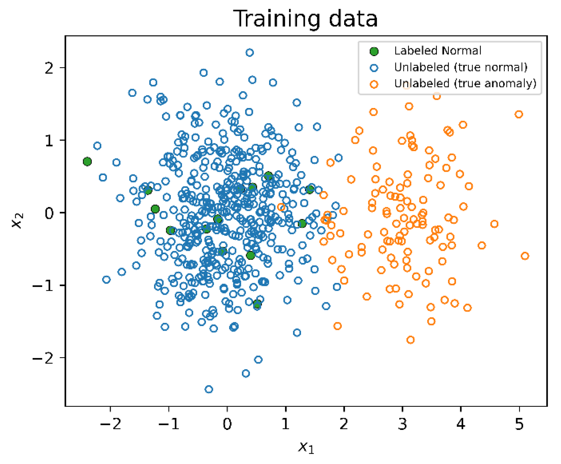
Figure 2.
GAR-DSVDD and benchmarking methods decision boundaries at testing over the simulated dataset. The proposed method achieves the best decision boundary that well represents the normal region by taking into account unlabeled data information by utilizing its attention-based graph and its deep structure.
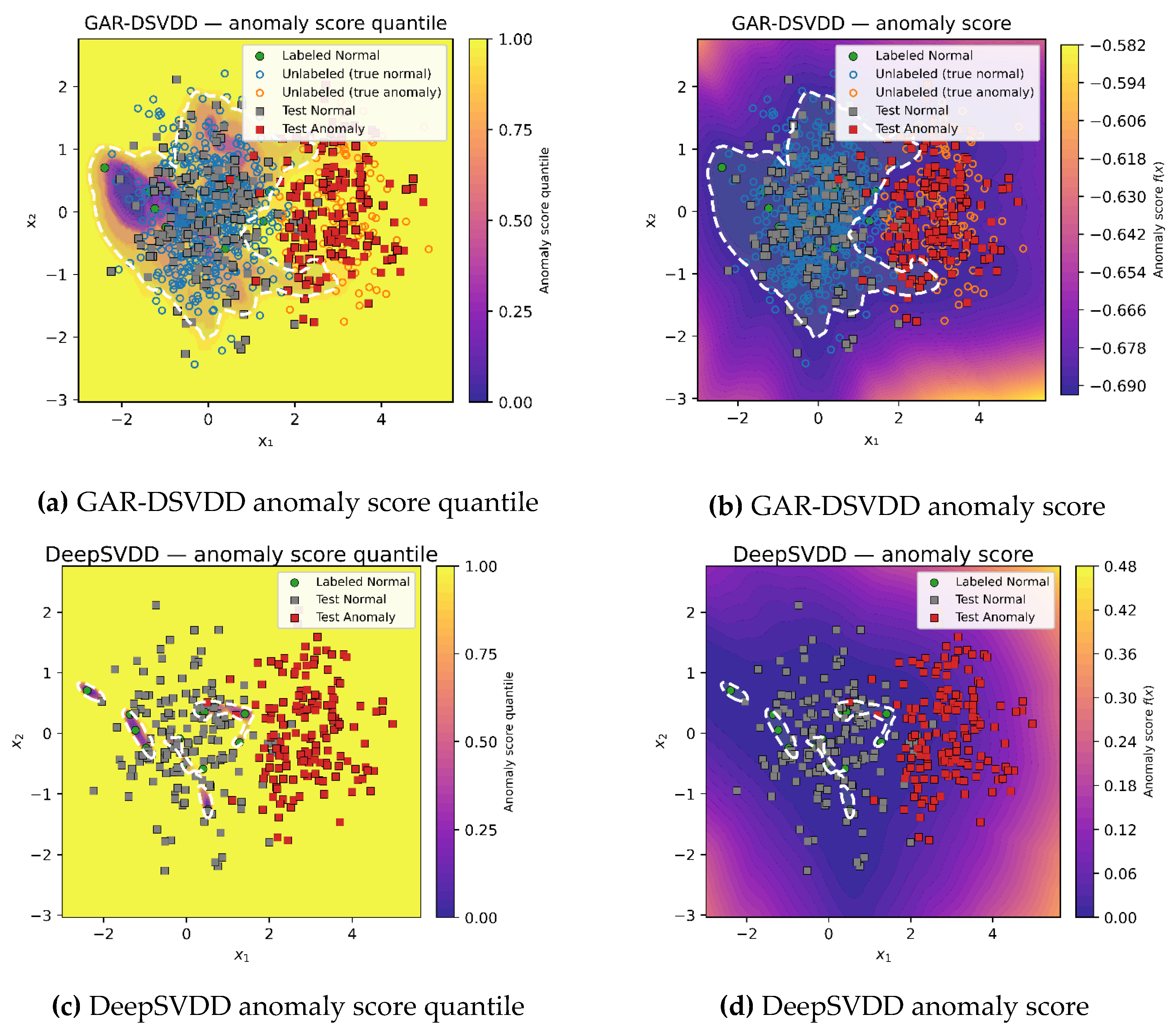
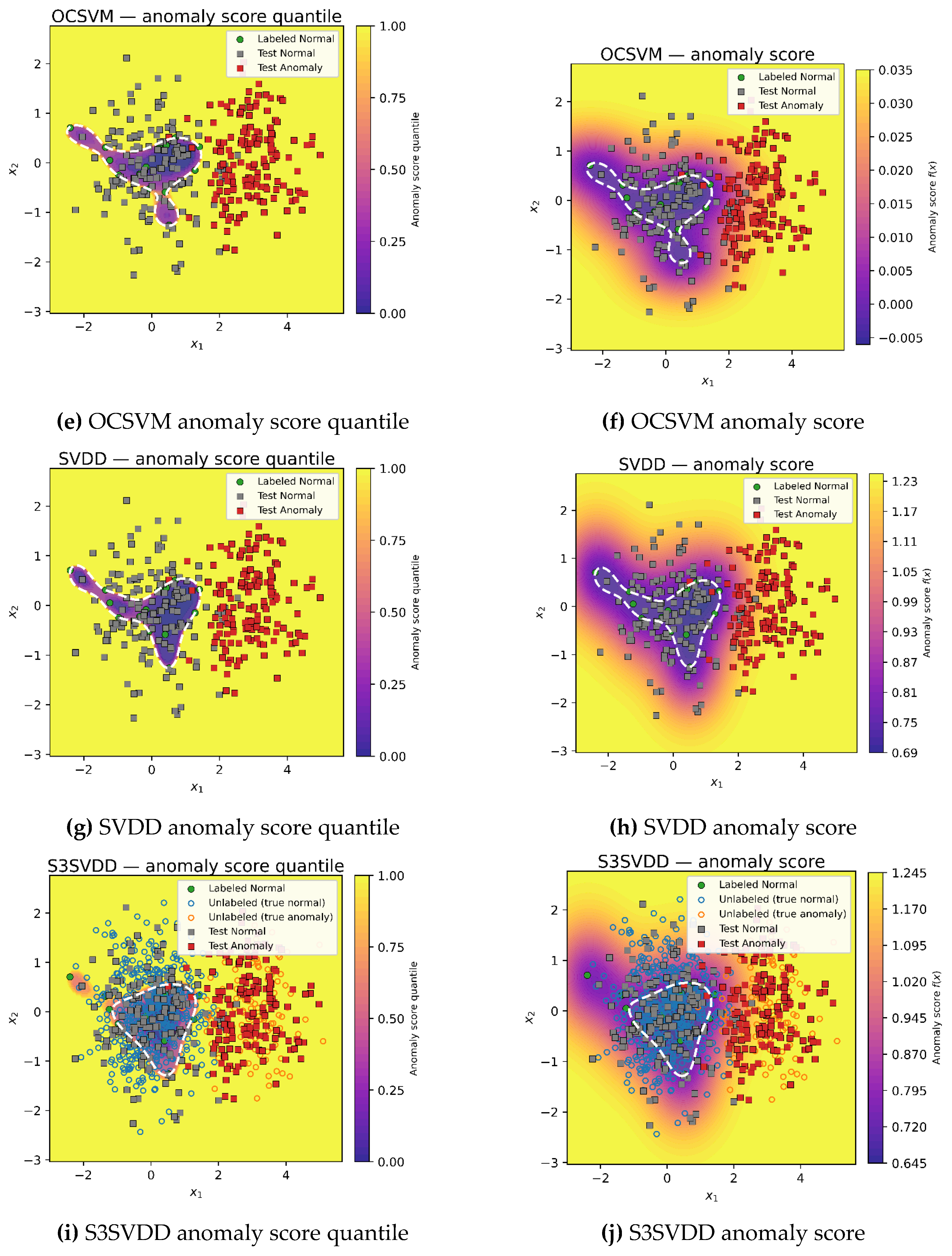
Figure 3.
An illustration of the windshield wipers sound recording and their MFCC features.
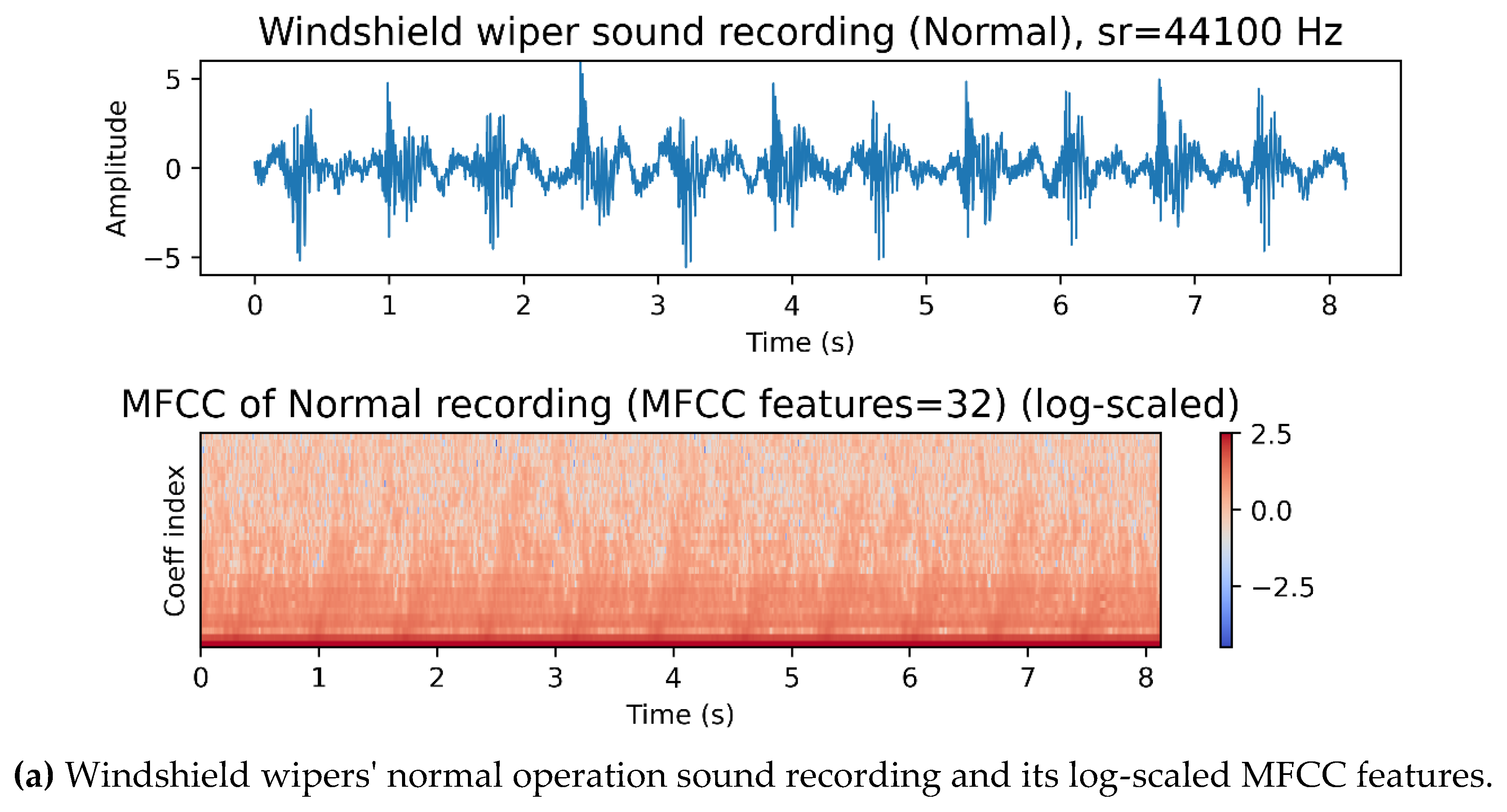
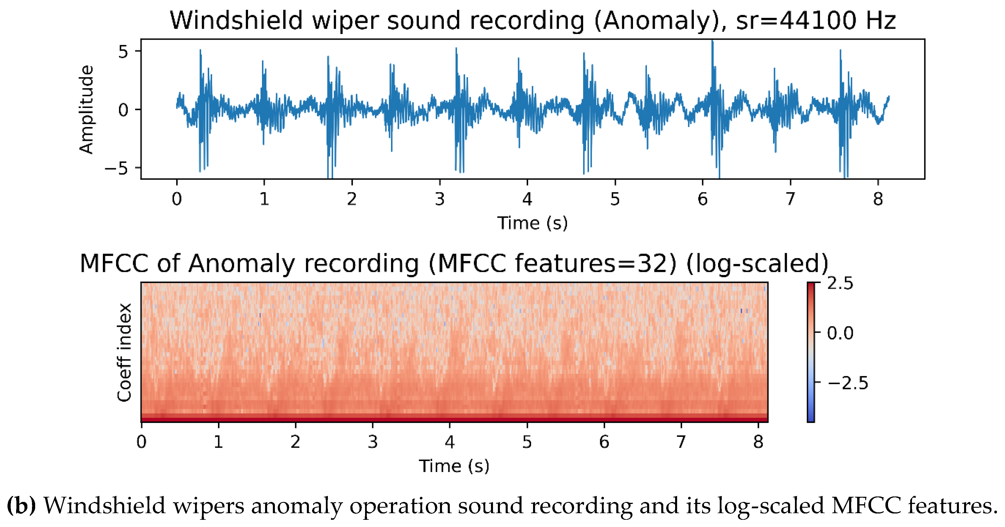
Figure 4.
Test F1 vs. . GAR-DSVDD leads when labels are scarce () and stays competitive, while DeepSVDD improves with more labels. OCSVM rises steadily but trails; SVDD is lowest; S3SVDD is non-monotonic (dip at ).
Figure 4.
Test F1 vs. . GAR-DSVDD leads when labels are scarce () and stays competitive, while DeepSVDD improves with more labels. OCSVM rises steadily but trails; SVDD is lowest; S3SVDD is non-monotonic (dip at ).
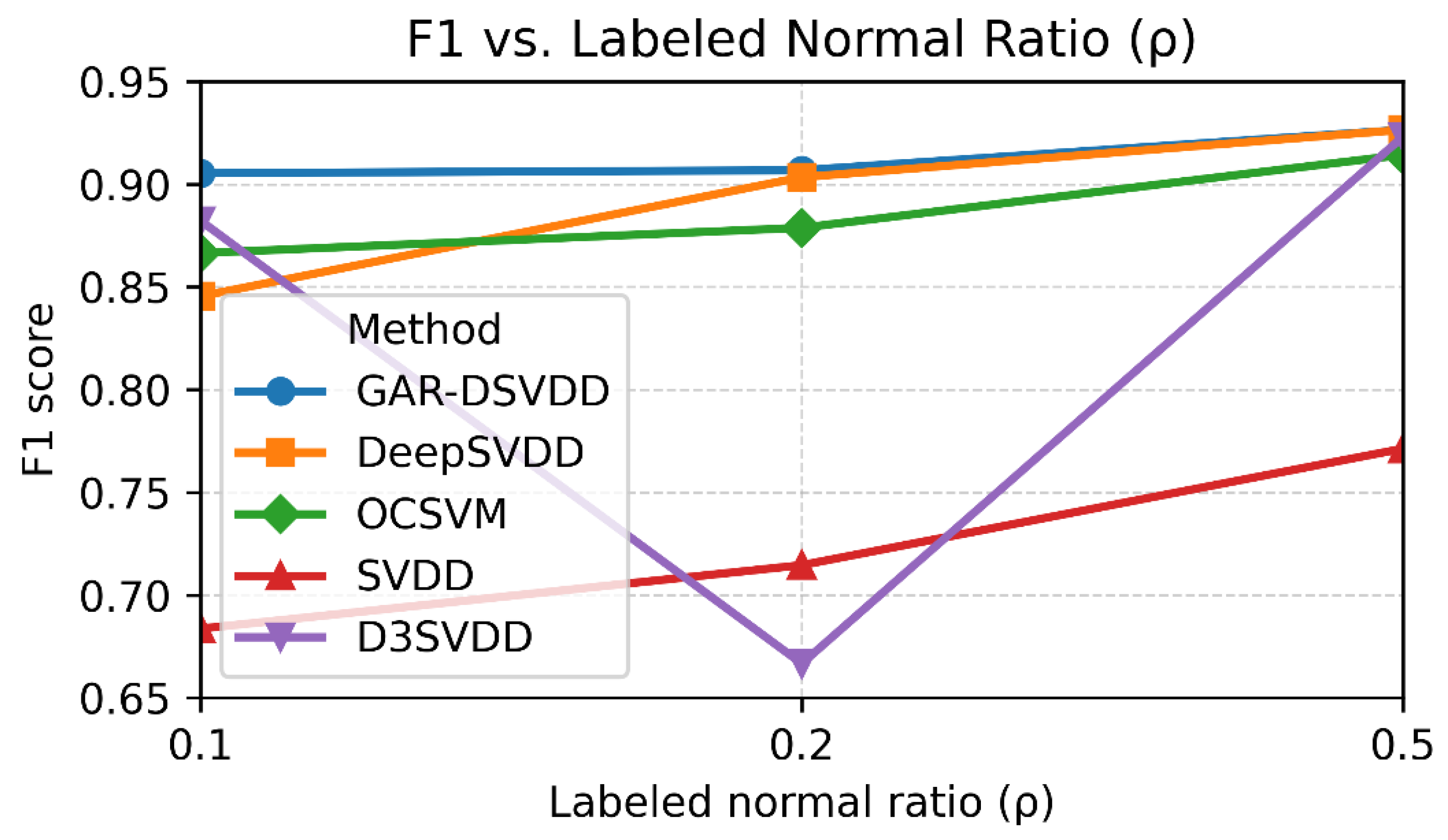
Figure 5.
Effect of on GAR-DSVDD performance at . Both F1 (left axis) and accuracy (right axis) improve as increases from 1 to 1300, peaking near , then declining for larger values, indicating over-regularization beyond the optimum.
Figure 5.
Effect of on GAR-DSVDD performance at . Both F1 (left axis) and accuracy (right axis) improve as increases from 1 to 1300, peaking near , then declining for larger values, indicating over-regularization beyond the optimum.
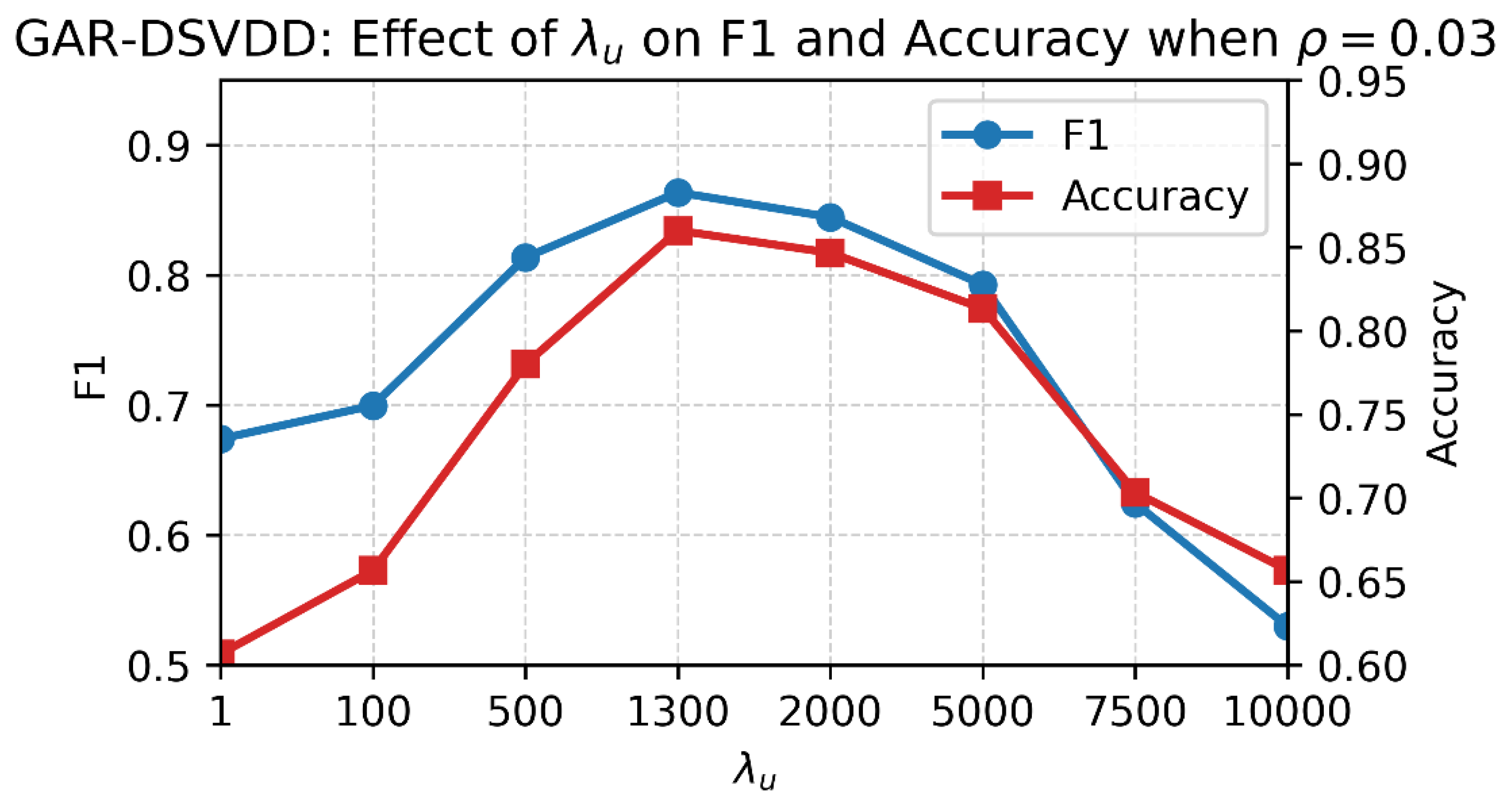

Table 1.
GAR-DSVDD and benchmark methods testing performance over a simulated dataset experiment.
| Method | Accuracy | F1 | Detection Rate |
Precision | Specificity | Balanced Accuracy |
|---|---|---|---|---|---|---|
| GAR-DSVDD | 0.92 | 0.92 | 0.99 | 0.86 | 0.84 | 0.92 |
| DeepSVDD | 0.56 | 0.69 | 1.00 | 0.53 | 0.11 | 0.56 |
| OCSVM | 0.76 | 0.81 | 0.99 | 0.68 | 0.53 | 0.76 |
| SVDD | 0.71 | 0.77 | 0.99 | 0.63 | 0.43 | 0.71 |
| S3SVDD | 0.69 | 0.76 | 0.99 | 0.62 | 0.38 | 0.69 |
Table 2.
GAR-DSVDD and benchmark methods testing F1 score over 10 simulated dataset experiments.
| Experiment (over different seeds) |
GAR-DSVDD | DeepSVDD | OCSVM | SVDD | S3SVDD |
|---|---|---|---|---|---|
| 1 | 0.86 | 0.68 | 0.74 | 0.74 | 0.74 |
| 2 | 0.83 | 0.70 | 0.78 | 0.78 | 0.78 |
| 3 | 0.80 | 0.73 | 0.80 | 0.70 | 0.70 |
| 4 | 0.92 | 0.69 | 0.81 | 0.77 | 0.76 |
| 5 | 0.88 | 0.69 | 0.75 | 0.67 | 0.67 |
| 6 | 0.80 | 0.72 | 0.80 | 0.79 | 0.79 |
| 7 | 0.81 | 0.69 | 0.76 | 0.68 | 0.69 |
| 8 | 0.86 | 0.68 | 0.79 | 0.75 | 0.74 |
| 9 | 0.78 | 0.69 | 0.76 | 0.76 | 0.76 |
| 10 | 0.85 | 0.68 | 0.76 | 0.77 | 0.77 |
| Mean | 0.84 | 0.70 | 0.78 | 0.74 | 0.74 |
| Standard deviation | 0.04 | 0.02 | 0.02 | 0.04 | 0.04 |
| p-value (Wilcoxon) | - | ||||
| p-value (paired t-test) | - |
Table 3.
Extracted features summary for acoustic analysis of windshield wiper operation sound recording.
Table 3.
Extracted features summary for acoustic analysis of windshield wiper operation sound recording.
| Feature family | Recording dimension (means & standard deviations)* |
Brief description | Reference |
|---|---|---|---|
| MFCC (32) | 64 | Cepstral summary of spectral envelope on the mel scale, a widely adopted baseline in recent ESC/SER studies. | [33,34] |
| ΔMFCC (32) | 64 | First-order derivative of MFCCs capturing short-term spectral dynamics. | [34] |
| Δ²MFCC (32) | 64 | Second-order derivative (acceleration) of MFCCs, emphasizing rapid spectral change. | [34] |
| Chroma (12) | 24 | Energy folded into 12 pitch-class bins; it reflects tonal/resonant structure seen in mechanical acoustics. | [33,34] |
| Spectral centroid | 2 | Power-weighted mean frequency (proxy for “brightness”). | [33,34] |
| Spectral bandwidth | 2 | Spread around the centroid (spectral dispersion). | [33] |
| Spectral roll-off (95%) | 2 | Frequency below which 95% of energy lies (high-frequency content indicator). | [33,34] |
| RMS energy | 2 | Framewise signal power (overall loudness proxy). | [33,34] |
| ZCR | 2 | Sign-change rate (simple proxy for roughness/high-frequency content). | [33,34] |
*Total observation dimension:
Table 4.
GAR-DSVDD and benchmark methods testing performance over the industrial windshield wiper dataset.
Table 4.
GAR-DSVDD and benchmark methods testing performance over the industrial windshield wiper dataset.
| Method | Accuracy | F1 | Detection Rate |
Precision | Specificity | Balanced Accuracy |
|---|---|---|---|---|---|---|
| GAR-DSVDD | 0.92 | 0.91 | 1 | 0.83 | 0.86 | 0.93 |
| DeepSVDD | 0.42 | 0.59 | 1 | 0.42 | 0 | 0.5 |
| OCSVM | 0.42 | 0.59 | 1 | 0.42 | 0 | 0.5 |
| SVDD | 0.42 | 0.59 | 1 | 0.42 | 0 | 0.5 |
| S3SVDD | 0.42 | 0.59 | 1 | 0.42 | 0 | 0.5 |
Table 5.
GAR-DSVDD and benchmark methods testing F1 score over 10 industrial windshield wiper experiments where different seeds are used to split the dataset into training, validation, and testing.
Table 5.
GAR-DSVDD and benchmark methods testing F1 score over 10 industrial windshield wiper experiments where different seeds are used to split the dataset into training, validation, and testing.
| Experiment (over different seeds) |
GAR-DSVDD | DeepSVDD | OCSVM | SVDD | S3SVDD |
|---|---|---|---|---|---|
| 1 | 0.86 | 0.55 | 0.55 | 0.55 | 0.55 |
| 2 | 0.93 | 0.8 | 0.8 | 0.82 | 0.8 |
| 3 | 0.76 | 0.5 | 0.5 | 0.52 | 0.5 |
| 4 | 0.79 | 0.60 | 0.63 | 0.63 | 0.63 |
| 5 | 0.67 | 0.63 | 0.63 | 0.63 | 0.63 |
| 6 | 0.91 | 0.59 | 0.59 | 0.59 | 0.59 |
| 7 | 0.83 | 0.45 | 0.45 | 0.45 | 0.45 |
| 8 | 0.97 | 0.74 | 0.74 | 0.74 | 0.74 |
| 9 | 0.96 | 0.7 | 0.7 | 0.7 | 0.7 |
| 10 | 0.90 | 0.63 | 0.63 | 0.69 | 0.63 |
| Mean | 0.86 | 0.62 | 0.62 | 0.63 | 0.62 |
| Standard deviation | 0.10 | 0.11 | 0.11 | 0.11 | 0.11 |
| p-value (Wilcoxon) | - | ||||
| p-value (paired t-test) | - |
Table 6.
Effect of Labeled-Normal Ratio () on F1 for GAR-DSVDD and benchmarks (DeepSVDD, OCSVM, SVDD, S3SVDD).
Table 6.
Effect of Labeled-Normal Ratio () on F1 for GAR-DSVDD and benchmarks (DeepSVDD, OCSVM, SVDD, S3SVDD).
| GAR-DSVDD | DeepSVDD | OCSVM | SVDD | S3SVDD | |
|---|---|---|---|---|---|
| 0.1 | 0.91 | 0.85 | 0.87 | 0.68 | 0.88 |
| 0.2 | 0.91 | 0.90 | 0.88 | 0.71 | 0.77 |
| 0.5 | 0.93 | 0.93 | 0.91 | 0.77 | 0.90 |
Disclaimer/Publisher’s Note: The statements, opinions and data contained in all publications are solely those of the individual author(s) and contributor(s) and not of MDPI and/or the editor(s). MDPI and/or the editor(s) disclaim responsibility for any injury to people or property resulting from any ideas, methods, instructions or products referred to in the content. |
© 2025 by the authors. Licensee MDPI, Basel, Switzerland. This article is an open access article distributed under the terms and conditions of the Creative Commons Attribution (CC BY) license (http://creativecommons.org/licenses/by/4.0/).
Copyright: This open access article is published under a Creative Commons CC BY 4.0 license, which permit the free download, distribution, and reuse, provided that the author and preprint are cited in any reuse.


