Submitted:
28 November 2025
Posted:
02 December 2025
You are already at the latest version
Abstract
Einstein’s general theory of relativity predicts that a difference in the gravitational potentials between two locations in a gravitational field would introduce a redshift or blueshift for a light ray travelling from one location to another. However, observations made in our solar system, such as the 21-cm radiation line from Taurus A near occultation by the Sun1, the Pioneer-6 spacecraft experiments2 and the solar limb effect3,4, clearly demonstrate that there exist anomalous redshifts which could not be explained by current theories and models. Here we show that beside the well-known Einstein gravitational redshift which has been verified by various observations, there exists an extra gravitational redshift which is caused by the change of photon’s momentum produced in a curved spacetime. We demonstrate that this type of gravitational redshift is just the super-gravity redshift as has been expected in literature. We derive a mathematical expression of the super-gravity redshift by using a theoretical model: a photon moving in a static Schwarzschild geometry, then apply it to calculate the centre-to-limb redshift variations across the solar disk. It is found that the redshift distribution predicted by the theoretical model agrees well with one of the observed profiles of the solar spectrum lines around 6300 , which demonstrates that the extra gravitational redshift should be the mechanism behind the solar limb effect and other observed anomalous redshifts.
Keywords:
photons
; redshift
; gravitational field
Introduction
With the fast development of advanced technologies and instrumentations, more and more effects predicted by Einstein’s general theory of relativity have been verified experimentally or confirmed by observations. The most recent examples shall include the detections of gravitational waves [5] and Lense–Thirring frame dragging effect [6]. However, there are still other phenomena and observations in astronomy and astrophysics which could not be explained by the general theory of relativity so far. One of them is the anomalous redshifts detected in number of astronomical observations including the 21-cm radiation line from Taurus A near occultation by the Sun [1], the Pioneer-6 spacecraft experiments [2] and the solar limb effect [3,4].
The variations of the wavelengths of Fraunhofer lines in the solar spectrum were observed back to a century ago. Since then intensive and systemic measurements and investigations on this matter have been carried out [7,8]. According to the general theory of relativity, a wavelength shift of the lines in the solar spectrum with respect to the corresponding lines from a low pressure laboratory source by an amount of is expected and this redshift should be independent on the locations on the whole solar disk since the gravitational potential generated by the Sun is equal on the solar disk. Even though different solar spectrum lines have shown different centre-to-limb variation features, it is an established fact that near the solar limb the Fraunhofer lines exhibit redshifts which substantially exceed the values predicted by the general theory of relativity and other activities in the solar atmosphere cannot account for. This phenomenon is called the solar limb effect in literature.
In order to explain the solar limb effect and the other anomalous redshifts detected in various astronomical observations and experiments, a large number of theories and models have been developed, and various theoretical interpretations have been proposed. In a series of studies on the interaction between photons and gravitational fields, it was postulated that under the influence of a gravitational field, a photon can decay into three or more secondary photons with one or more gravitons and, hence the original photon will gradually lose its energy and its frequency decreases [9,10]. The developed theory can explain some of the observed phenomena, however, the proposed photon decay process still remains as a hypothesis even at the present time. In another work, it was shown that the interaction between an electromagnetic field and a gravitational field would cause the electromagnetic wave to change its frequency while travelling through a combination of the two fields [11]. A laboratory experiment with a two-beam laser interferometer carried out immediately after the publication of the above theory provided a negative result [12]. The solar atmosphere contains various particles including electrons and ions, therefore, interactions between photons and the charged particles have been considered and modelled for interpreting the anomalous redshifts detected in the observations associated with the Sun [13,14]. The interaction between photons and light neutral bosons emitted by the Sun as well as light wave propagating in inhomogeneous media have also been proposed [15,16]. Other exotic explanations, such as non-zero photon rest mass and variable speed of light have ever been considered although these assumptions are inconsistence with the fundamental principles of physics [17,18,19,20].
After decades of research (particularly in 60s and 70s), so far there is still no consistent and satisfactory explanation to the solar limb effect and other anomalous redshifts, and an orthodox theory without ad hoc hypothesises and assumptions is still lacking.
Here, by utilizing the fundamental principles in general relativity, we show that when a photon travels in a curved spacetime the photon’s momentum is not necessarily conserved for a local rest observer along the photon’s trajectory and, therefore, an extra redshift will be produced. This type of redshift is completely different from the conventional gravitational redshift (also called the Einstein redshift) which is determined by the difference in the gravitational potentials between an emitter and a receiver. This redshift is caused by the change of photon’s momentum which is related to the bending of the photon’s trajectory in the curved spacetime. We apply the derived formula to calculate the redshift distribution across the solar disk and find that the results agree well with the observed data taken from the week Fraunhofer lines around 6300 , which demonstrates this additional redshift could be the key for explaining the century-long solar limb effect and other anomalous redshifts observed in our solar system.
Photon Motion in Gravitational Field
According to the general theory of relativity, the motion of a massive particle which has a non-zero rest mass and experiences no other external forces except gravity will follow a geodesic and the equations of motion are given by [21]
where the proper time is used as the affine parameter.
Massless particles, like photons which are the particles that make up light and have zero mass, can be treated in a similar way in general relativity when their motions in gravitational fields are investigated. As well known, Eq.1 cannot be used for massless particles since a massless particle is moving at the speed of light with a lightlike worldline, and its motion is described by a null geodesic for which .
It has been shown that by using the variational approach and Lagrangian procedure, a generic expression of the geodesic equations for both massive and massless particles can be derived. For simplicity and without losing generality, here we will consider the situations where photons are in Schwarzschild geometry.
Constructing a Lagrangian
where and is an affine parameter, and substituting the Lagrangian into the Euler-Lagrange equations
we have
Here, there is no limit on the affine parameter in deriving the geodesic equations, and it is clear that when the proper time is selected as the affine parameter, Eq.1 is obtained. In Schwarzschild geometry, the metric is given by [22]
whereas the speed of light c is set to 1.
Then, the Lagrangian can be calculated as
For photons, . Since a static Schwarzschild metric does not depend on the coordinate time and the azimuthal angle φ, from Eq. 6, we have
We therefore obtain two important constants of motion: the energy and the angular momentum
This means that both the energy and the angular momentum are conserved for a particle (either massive or massless) moving along a geodesic in the static Schwarzschild spacetime. It is worth to stress here that both the energy and the angular momentum are quantities measured by a rest observer at infinity (i.e. ), and they are different from those observed by a local rest observer. This point is critically important and will have far-reaching consequences for our further analysis.
From the equation on , we also have
That is
By choosing and as the initial conditions, we thus have , which indicates that a particle moving in the equatorial plane will keep its motion in the plane. Since the Schwarzschild metric is the solution of Einstein’s field equations outside of a spherically symmetric mass distribution, one can always select a polar axis to ensure that the particle’s motion is in the equatorial plane. For the analysis follows, we assume that photons move in the equatorial plane of the Schwarzschild coordinates.
We know that a photon has an energy of and a linear momentum of , whereas is the reduced Planck constant, the angular frequency and c the speed of light (taking c=1). This implies that, for a photon, any changes in its energy, momentum and frequency are directly connected.
We now consider a stationary photon emitter E and a stationary photon receiver R positioned at space coordinates and respectively as shown in Figure 1. The worldlines of the emitter and the receiver are represented by the two straight lines labelled by and with and as their proper times. Suppose that at some event , E emits a photon with 4-momentum measured by a rest observer at A. The emitted photon propagates along its worldline and then reaches the receiver E at an event . The 4-momentum of the photon at B is which is observed by a rest observer at B and could be different from . The photon’s worldline follows a null geodesic which is generally curved because of the existence of the spacetime curvature as described by the Schwarzschild metric in Eq.5.
The photon energy measured by a rest local observer at A can be expressed as
where is the 4-velocity of the observer at A. Similarly, for a rest local observer at B, the measured photon energy can be written as
whereas is the 4-velocity of the observer at B. By using the energy-frequency relationship , we can calculate the ratio of frequencies observed at B and A as
The contravariant components of the 4-velocity of an ordinary object with a rest mass are given by , and satisfy . From the 4-velocity, one can also define the 4-momentum of the massive object as . By using these definitions, we can find the 4-velocities of the rest observers at A and B as
The 4-momentum of a photon is a vector which is tangent to photon’s geodesic at any point along its worldline and is parallel-transported along the path. The contravariant components of the 4-momentum of a photon are
where is 3-momentum of the photon.
When the photon moves in the equatorial plane of the Schwarzschild coordinates, the contravariant components of its 4-momentum are given by [23]
whereas b is the impact parameter of the incoming photon. By using the relationship , we can calculate the covariant components of photon’s 4-momentum. For the purpose of further developing Eq.14, we only need component. Now Eq.14 can be written as
As has been emphasized above, and are the photon momenta measured by the local rest observers at A and B respectively. It should be noted that has been utilized in all previous studies by applying the energy and momentum conservation rules derived from the fact of for a photon moving along its geodesic in the static Schwarzschild coordinates, and as we have stressed above, these conserved quantities are only for a rest observer at infinity.
By defining and , and also inserting the expressions for and for the Schwarzschild metric, we rewrite Eq. 22 as
where and are the radial coordinates of point A and B respectively.
For a weak gravitational field, and , we can expand Eq.23 by taking the first order approximation and obtain
Thus, by recovering the speed of light c, we find the expression for the redshift as
It is clear that the difference in radial coordinates between the emitter and the receiver will introduce a redshift. This redshift is caused by the time dilation in the curved spacetime and is well known in general relativity. A relationship expressing this effect can also be derived directly from the equivalence principle and is frequently explained as the difference in gravitational potentials between point A and point B. In general relativity, this type of redshift is normally called the Einstein gravitational redshift.
The most important point here is that any changes in photon’s momentum between the emitter and the receiver will also contribute to the total redshift. As the photon’s momentum is a vector and is always tangent to photon’s geodesic at any point along its worldline, any variation in the amplitude of momentum or the direction or both of them, should be taken into account.
For the change in direction by a small angle , we have . Thus, the change in photon’s momentum can be calculated from its bending angle when moving from point A to B along its trajectory.
In the equatorial plane of the Schwarzschild coordinates, a photon will follow a trajectory described by the geodesic equation, which is [21]
whereas b is the impact parameter at infinity. From this equation we obtain an expression for the deflection angle of a photon traveling from to as
where is closest approach of the photon trajectory to the coordinate origin, and in a weak gravitational field . With Eqs. 25 and 27, the total redshift for a photon traveling between any two points in the equatorial plane of the Schwarzschild coordinates can be calculated. Although the integral in Eq.27 can be completed for some special cases, generally the deflection angle can only be calculated by using numerical methods.
For and , we have the well-known result [24] . In this case, the conventional Einstein gravitational redshift vanishes, but the additional gravitational redshift remains if .
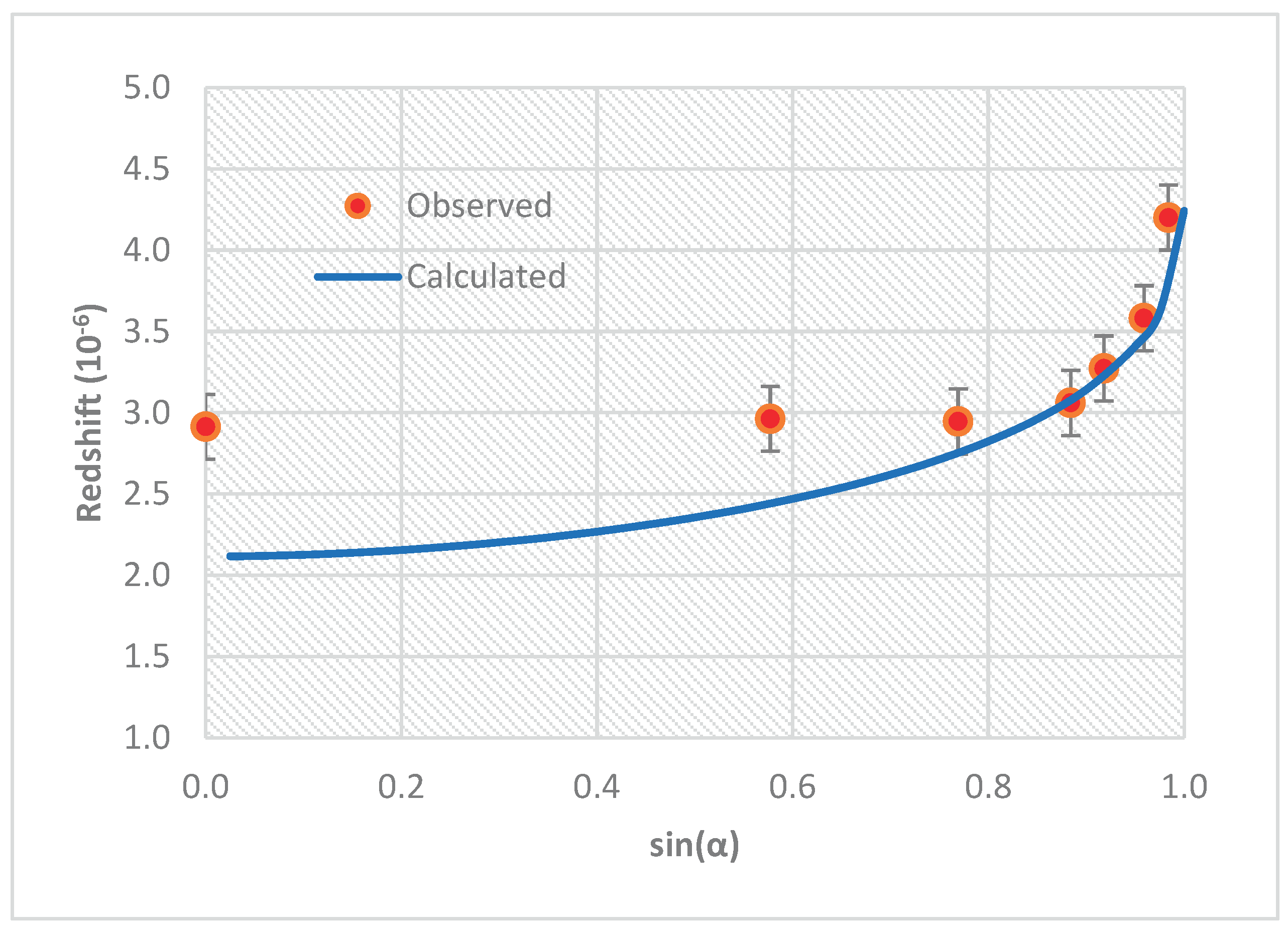
We calculated the redshift distribution across the solar disk by considering an emitter (point A) on the solar disk and a receiver (point B) at earth and the results are shown in Figure 2. It can be seen that the redshift gradually increases from the centre to the edge and reaches its maximum at the solar limb. In Figure 2, we also show a group of published data which were obtained by measuring the redshifts of the solar spectrum lines around 6300 (Ref.3). In this particular measurement, the redshift at the centre of the solar disk is about which is less than the Einstein redshift of generated by the Sun’s gravitational field. The reason could be that the radial motions in the solar atmosphere generate blueshifts which cancel part of the gravitational redshift. Also one cannot establish exactly the zero-line of the wavelength variations. Therefore, for comparison purpose, we move the observed data by . From Figure 2, we can see that the calculated redshift distribution matches the measured centre-to-limb profile for the selected spectrum lines particularly in the area close to the solar limb.
Conclusion
In summary, we demonstrate that there exists an additional gravitational redshift for a photon travelling in a curved spacetime beyond the conventional Einstein gravitational redshift which is completely determined by the difference in the gravitational potentials between the photon’s emitter and receiver. This redshift arises from the change of photon’s momentum along its curved trajectory under the influence of a gravitational field. The underline principle is that in general relativity the energy and momentum of a photon moving in a curved static spacetime will be conserved only for a rest observer at infinity. By utilizing the fundamental principles and equations from the general theory of relativity, we derive an expression of the additional redshift in the static Schwarzschild coordinates and, as an application, we apply it to calculate the centre-to-limb redshift variations across the solar disk. We show that the derived expression of the additional redshift provides a concrete theoretical explanation not only for the solar limb effect but also for other observed anomalous redshifts for which detailed calculations and analyses will be carried out in future research.
References
- Sadeh, D., Knowles, S. H. & Yaplee, B. S. Search for a frequency shift of 21-centimeter line from Taurus a near occultation by sun. Science 159, 307-308 (1968).
- Goldstein, R. M. Superior conjunction of ioneer-6. Science 166, 598-601 (1969).
- Adam, M. G., Interferometric measurements of solar wave-lengths and an Investigation of the Einstein gravitational displacement. Monthly Notices of the Royal Astronomical Society 108, 446-464 (1948).
- Adam, M. G., A new determination of the centre to limb change in solar wave-lengths. Monthly Notices of the Royal Astronomical Society 119, 460-474 (1959).
- Abbott, B. P. et al. Observation of Gravitational Waves from a Binary Black Hole Merger. Physical Review Letters 116, (2016). [CrossRef]
- Krishnan, V. V. et al. Lense-Thirring frame dragging induced by a fast-rotating white dwarf in a binary pulsar system. Science 367, 577-580 (2020).
- Adam, M. G., Ibbetson, P. A. & Petford, A. D. Solar limb effect - observations of line contours and line shifts. Monthly Notices of the Royal Astronomical Society 177, 687-708 (1976).
- Plaskett, H. H. Solar wavelengths and limb effect. Monthly Notices of the Royal Astronomical Society 179, 339-350 (1977).
- Crawford, D. F. Interaction of a photon with a gravitational-field. Nature 254, 313-314 (1975).
- Crawford, D. F. Photon decay in curved space-time. Nature 277, 633-635 (1979).
- Szekeres, G. Effect of gravitation on frequency. Nature 220, 1116-1118 (1968).
- Shamir, J. Experimental test of a gravitational effect suggested by Szekeres. Nature 222, 362-362 (1969).
- Marmet, P. Red shift of spectral-lines in the sun’s chromosphere. IEEE Transactions on Plasma Science 17, 238-244 (1989).
- Accardi, L., Laio, A., Lu, Y. G. & Rizzi, G. A third hypothesis on the origin of the redshift: Application to the Pioneer 6 data. Physics Letters A 209, 277-284 (1995).
- Merat, P., Pecker, J. C. & Vigier, J. P. Possible interpretation of an anomalous redshift observed on the 2292 MHz line emitted by Pioneer-6 in the close vicinity of the solar limb. Astronomy & Astrophysics 30, 167-174 (1974).
- Ferencz, C. & Tarcsai, G. Theoretical explanation of the solar limb effect. Planetary and Space Science 19, 659-667 (1971).
- Pecker, J. C., Vigier, J. P. & Roberts, A. P. Non-velocity redshifts and photon-photon interactions. Nature 237, 227-229 (1972).
- Woodward, J. F. & Yourgrau, W. A paradox in the interaction of the gravitational and electromagnetic fields. Nature 226, 619-621 (1970).
- Woodward, J. F. & Yourgrau, W. Difficulties concerning a finite photon rest mass. Nature 241, 338-338 (1973).
- Wilhelm, K. & Dwivedi, B. N. Gravitational redshift and the vacuum index of refraction. Astrophysics and Space Science 364, doi:10.1007/s10509-019-3513-4 (2019).
- Hobson, M. P., Efstathiou, G. & Lasenby, A. N. General relativity: an introduction for physicists. (Cambridge University Press, 2006).
- Hartle, J. B. Gravity: an introduction to Einstein's general relativity. (Addison-Wesley, 2003).
- Moore, T. A. A general relativity workbook. (University Science Books, 2013).
- Weinberg, S. Gravitation and cosmology: principles and applications of the general theory of relativity. (Wiley, 1972).
Figure 1.
A schematic diagram illustrating the spacetime outside a static and spherically symmetric mass. A stationary emitter located at point A emits a photon and a rest receiver at point B detects the photon. The worldlines of the emitter and the receiver are represented by two straight lines with their lightcones indicated. The photon’s trajectory follows its geodesic and is curved. and are the photon’s momenta at point A and B respectively, and are not necessary equal to each other in the curved spacetime.
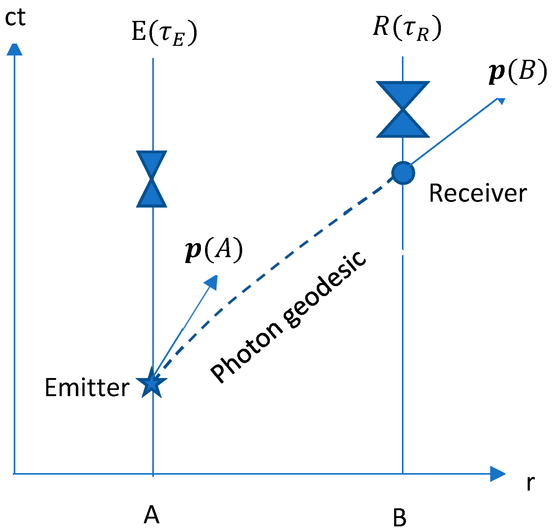
Figure 2.
Calculated redshift distribution across the solar disk and observed data from a solar spectrum lines around 6300 (Ref.3). The redshifts are presented as functions of representing the positions on the solar disk, where is the angle between the line of sight and the radius connecting the observed point with the centre of the Sun. For comparison purpose, the observed data are shifted by which is the theoretical Einstein gravitational redshift at the centre of the Sun.
Disclaimer/Publisher’s Note: The statements, opinions and data contained in all publications are solely those of the individual author(s) and contributor(s) and not of MDPI and/or the editor(s). MDPI and/or the editor(s) disclaim responsibility for any injury to people or property resulting from any ideas, methods, instructions or products referred to in the content. |
© 2025 by the authors. Licensee MDPI, Basel, Switzerland. This article is an open access article distributed under the terms and conditions of the Creative Commons Attribution (CC BY) license (http://creativecommons.org/licenses/by/4.0/).
Copyright: This open access article is published under a Creative Commons CC BY 4.0 license, which permit the free download, distribution, and reuse, provided that the author and preprint are cited in any reuse.


