
Submitted:
29 November 2025
Posted:
02 December 2025
You are already at the latest version
Abstract
This study investigates how U.S. Federal Reserve interest rate cuts during the 2019–2020 easing cycle influenced the performance of equity mutual funds, with a focus on con-trasting growth and value strategies. Using an event study framework, we examine abnormal returns (AR), cumulative abnormal returns (CAR), and risk-adjusted perfor-mance measured by both static and rolling (30-day) Jensen’s alpha () and Sharpe ratios (SR) across short-term (30-day) and long-term (6-month and 1-year) windows surrounding three major rate cut events.
Further statistical tests reveal that growth funds significantly outperform value funds following rate reductions, especially over longer horizons. This performance premium is more pronounced in risk-adjusted returns and becomes stronger when accounting for rolling dynamics, indicating that growth funds are more responsive and sensitive to monetary easing. These findings underscore a persistent and asymmetric sensitivity of different fund styles to interest rate changes, shaped by differences in duration exposure and investor sentiment.
This study offers novel insights into how monetary policy influences fund-level dynamics beyond broad market movements and deepens the understanding of monetary trans-mission in asset management by incorporating time-varying performance metrics.
Keywords:
Federal Reserve
; interest rate cuts
; growth funds
; value funds
; abnormal returns
; Jensen’s alpha
; Sharpe ratio
; monetary policy transmission
MSC: 91G05, 91G80, 62P05
1. Introduction
Financial markets are greatly affected by monetary policy, especially through changes in the Fed’s funds rate. Interest rate cuts help lower capital costs, boost business investment, and stimulate consumer spending, all of which, taken together, help to boost equity market values. Bernanke and Blinder [1] and Taylor [2] discussed how changes in interest rates are transmitted to the real economy, which in turn affects financial markets and asset prices, from theoretical and empirical perspectives, respectively. Furthermore, Bernanke and Kuttner [3] empirically demonstrated that reductions in interest rates correlate with substantial positive responses in the stock market, principally via mechanisms such as equity risk premium compression and alterations in investor mood. While the impact of monetary policy on equity markets is well-documented, less is known about how different mutual fund investment types, including value funds and growth funds, react to these policy changes. By nature, growth funds invest in companies with great future profit potential; therefore, their values are quite sensitive to variations in the discount rate used for far future cash flows. Estep [4] used the Break-Even Time (BET) concept to show that high price-to-earnings (P/E) ratio stocks, which are usually high-growth companies, have a present value that is especially sensitive to changes in interest rates. In contrast, value stocks grounded in near-term earnings and stable dividends demonstrate greater resilience to such shifts, making them less sensitive to interest rate changes.
The concept of equity duration may explain this asymmetric sensitivity, since growth stocks can be viewed as longer-duration assets than value stocks [5]. Growth and value funds differ in their asset composition, cash flow profiles, and sensitivity to monetary policy shocks. Growth funds primarily invest in companies with higher expected earnings growth rates, as their value is primarily derived from cash flows over a longer period. Therefore, these funds are more sensitive to changes in discount rates [6]. This interest rate sensitivity comes from the discounted cash flow (DCF) model. In contrast, value funds invest in companies with stable earnings and undervalued fundamentals. Lower discount rates have less of an impact on value stocks, as their valuations are more dependent on short-term cash flows. Consequently, growth funds are more affected by interest rate cuts, while value funds react more moderately.
While this theoretical difference is commonly recognized, few empirical studies systematically examine the performance of different fund styles under real monetary shocks. Literature reviews reveal a lack of in-depth analysis of how mutual stock funds with distinct investment styles (e.g., growth funds and value funds) respond to interest rate changes. Previous research has largely focused on stock indices and bond markets, lacking empirical studies at the fund level that consider both raw and risk-adjusted returns over different periods. In addition, many studies neglect the fund’s response over time and typically do not use dynamic risk-adjusted performance measures.
We bridge these gaps by systematically investigating how the U.S. Federal Reserve’s interest rate cuts during the 2019–2020 easing cycle affected the performance of value and growth funds with different investment styles in equity mutual funds. The 2019 to 2020 interest rate cut cycle is worth studying because it occurred on the eve of the COVID-19 crisis, when interest rates were low and valuations were high. Unlike typical recession easing, this cycle involved proactive measures that were not driven by a crisis. This provides a unique opportunity to study how policy affects asset valuations. Applying an event study methodology, we analyze and compare the abnormal returns (AR) and cumulative abnormal returns (CAR) over the 30 days, 6 months, and 1 year preceding and following three critical policy events. In addition to raw returns, we also incorporate static and dynamic risk-adjusted measures, such as Sharpe ratio (SR), Jensen’s alpha (α), volatility, and beta (β) coefficients, with particular emphasis on their 30-day rolling versions to reflect fund dynamics under different periods and market changes. These rolling measures (30-day window) capture the time-varying dynamics of funds’ response to policy shocks. Finally, a set of regression models within the Capital Asset Pricing Model (CAPM) framework is constructed to separate the impact of monetary policy on different fund styles and investment horizons, while controlling systematic market risk. These are rarely seen in mutual fund literature, but they help us understand how funds behave over time. This method allows us to tell the difference between temporary volatility and persistent performance trends following policy changes. More detailed information is included in the “Methodology” section.
This dual-focus approach helps to more clearly distinguish between fund responses to interest rate changes at the discount rate and the broader impact of market-level monetary easing policies. Based on the DCF theory, which implies growth-oriented assets are interest-rate-elastic due to their reliance on future earnings, this analysis examines the extent to which such theoretical expectations manifest as enduring disparities in realized performance. Therefore, this study fills a gap in existing literature that seldom controls time-varying responses at the fund level or uses dynamic measures of performance. The findings offer empirical insights into transmission mechanisms of monetary policy at the fund level and contribute to portfolio strategy, fund risk management, and the broader understanding of how monetary policy shapes asset performance across different investment styles.
2. Literature Review
2.1. The Impact of Monetary Policy on Stock and Fund Markets
Macroeconomic factors like inflation, GDP growth, and employment have a significant impact on financial markets, especially through monetary policy. Although monetary policy typically operates with a lag, stock and fund markets often react swiftly to anticipated interest rate changes.
Jayawickrema [7] distinguished between conventional and unconventional monetary policies. This study finds that adjustments in the federal funds rate drive broad market returns. In contrast, unconventional tools, like forward guidance and large-scale asset purchases (LSAPs), significantly impact U.S. stock returns across sectors. Similarly, Hojat and Sharifzadeh [8] used a multi-factor Capital Asset Pricing Model (CAPM) to demonstrate that monetary instruments, such as money supply (M2), federal funds rate (FFR), and federal funds futures (FFF), significantly influence firm-level returns and investor behavior. The responses of financial markets may also influence future policy decisions. However, most of these studies focus on aggregate market indices or individual stocks, with limited exploration of mutual fund responses, especially among different investment styles.
Despite extensive research on how monetary policy affects equity markets, there is still little evidence on how mutual funds, especially those with varying investment styles, respond. This study aims to fill that gap by looking at the performance of value and growth funds during monetary easing.
2.2. Performance Difference Between Growth and Value Funds
Growth and value equity funds react differently to changes in interest rates because of the types of their underlying assets. Growth funds invest in firms with high earning potential and long-term cash flows, which makes their valuations highly sensitive to discount rates. As a result, they usually gain more from monetary easing. In contrast, value funds invest in established firms with stable cash flows and lower valuations, which makes them less affected by rate changes [6,9,10].
Fama and French [10] introduced the three-factor model, which includes market, size, and book-to-market ratios, to explain variations in stock returns. Their findings show that growth stocks perform better during expansionary periods. More defensive value stocks provide better stability during market downturns. To better capture return drivers, Fama and French [11] later expanded this into a five-factor model, adding profitability and investment factors. The five-factor model further improves explanatory power, especially in distinguishing growth versus value dynamics by accounting for differences in operating performance and reinvestment behavior.
However, these models have mainly been applied to conventional economic environments. The behavior of growth and value funds during unconventional monetary conditions, such as sharp or unexpected rate cuts, has not been thoroughly examined. Existing studies rarely explore whether the performance of these fund styles varies across different time horizons or during elevated volatility.
This study addresses this gap by investigating how growth and value mutual funds react to interest rate cuts using both static and dynamic risk-adjusted measures. By combining traditional models with rolling measures, it explores whether growth funds consistently perform better under easing conditions and whether these effects persist or diminish over time.
2.3. Interest Rate Policy and Risk-Adjusted Performance
Monetary policy, especially changes to the federal funds rate, is crucial in influencing asset prices and fund performance. Bernanke and Kuttner [3] demonstrated that an unexpected 25-basis-point change in the federal funds rate can lead to a 1% shift in stock market returns in a single day. Their event study, which used federal funds futures data, reveals that these reactions are mainly driven by revised expectations of future earnings, not by shifts in real interest rates or cash flows. Further analysis using a structural vector autoregression (VAR) model revealed that unexpected monetary shocks exacerbate market volatility and reshape the transmission path from policy to asset prices.
At the fund level, interest rate cuts have been found to enhance equity market returns and smooth the growth of funds that outperform value funds. This aligns with the higher sensitivity of growth-oriented portfolios to duration and discount rates. Elton et al. [12] discovered that historical alpha can strongly predict future risk-adjusted returns, especially for top-performing funds. Recent studies have explored that funds maintain solid performance in volatile markets when fund managers effectively handle systemic risk [13].
The development of performance metrics has enhanced our understanding of fund behavior. Sharpe [14] introduced the Sharpe ratio, a standard measure that assessed excess return per unit of total risk. Jensen [15] later suggested Jensen’s alpha, which reflects a fund manager’s ability to generate returns above the CAPM benchmark. Both metrics are fundamental in evaluating the fund’s efficiency. Roll [16] improved this further by incorporating dynamic risk structures, indicating that SRs for growth funds often rise significantly after rate cuts due to their heightened sensitivity to market shifts.
Smith and Tito [17] compared performance metrics and found that the Traynor volatility ratio was better for highly diversified funds. In contrast, the SR and α gave more consistent rankings. They used a CAPM regression framework to evaluate fund rankings under each index. This highlighted the need to select the appropriate metrics for measuring risk-adjusted performance across various fund styles.
However, performance persistence also depends on broader market conditions. Rahayu et al. [18] argued that during high market risk, changes in interest rates have a limited influence on fund returns. While the LQ45 index did not moderate the impact of inflation, it significantly lessened the negative impact of interest rates and market volatility on performance.
To address the drawbacks of conventional metrics during zero-lower-bound policy regimes, Eksi and Tas [19] introduced using the shadow federal funds rate as a proxy. Their study demonstrated that unconventional tools like large-scale asset purchases (LSAPs) triggered portfolio rebalancing from bonds to equities, intensifying the sensitivity of stock returns to monetary policy.
In conclusion, the literature confirms that an exhaustive understanding of fund responses to changes in interest rates requires both raw and risk-adjusted return assessments. Several static and dynamic measures, including volatility, SR, and α, among them, shed important light on the time-varying nature of fund performance. Upon this foundation, the present study uses an event study design to investigate the responses of growth and value mutual funds to the 2019 Fed decreases in rates. Through the combination of both rolling and static risk-adjusted measures, this study explores not just the average but also the persistence and the timing involved in the fund reactions to changes in the stance of monetary policy.
2.4. Short-Term and Long-Term Effects of Monetary Policy
The Fed’s monetary policy has immediate and persistent effects on different asset classes. Bond prices quickly respond to policy changes because they are sensitive to the term structure of interest rates. In contrast, equity markets mainly respond by adjusting expected risk premiums [20]. These different channels of response underscore the need to distinguish between short-term and long-term market reactions.
Empirical research confirms such temporal asymmetries. Research supports these time differences. Growth funds, which are highly sensitive to forward-looking expectations, tend to exhibit stronger short-term ARs after interest rate cuts. Value funds, which are anchored in stable fundamentals, respond more gradually [21]. This divergence reflects style-based differences in how monetary easing is priced in.
Studies in broader market contexts also confirm the time-sensitive response. Interest rate changes induce short-term volatility in Chinese equity markets; however, these changes are negatively correlated with long-term stock prices. Despite differences in institutions, the findings highlight the importance of modeling persistence and structural adjustment in market responses [22].
Furthermore, in the U.S., Marfatia [23] utilized a model with time-varying parameters (TVP) and discovered that short-term interest rates react more to monetary shocks than long-term rates, especially under elevated financial market uncertainty. Policy transmission dampened during stressful periods, reducing the long-term effectiveness of monetary interventions.
Similarly, Bjørnland and Leitemo [24] used a structural VAR approach to identify strong short-term effects of Fed rate hikes on equity indices such as the S&P 500 stock market, with impacts fading as markets re-anchor expectations. This reinforces the notion that effects of monetary policy on the stock market are inherently temporary, but these effects may diminish in the long run as market expectations adjust and initial euphoria subsides.
From the perspective of funds, growth funds react more in the short term, while value funds maintain steadier returns across horizons. This persistence established that value strategies depend less on rapid changes in expectations and are somewhat insulated from volatility [25].
Overall, these findings emphasize the need for a time-sensitive framework when analyzing fund reactions to monetary policy. Therefore, this study uses a multi-horizon event window, combining a short-term (30 days before and after the interest rate cut) and a long-term (6-month and 1-year intervals) event window to comprehensively assess the temporal dynamics of the responses of growth and value equity stock funds to the Fed’s rate cuts.
3. Methodology
3.1. Research Hypotheses
This study aims to clarify the following key hypotheses based on the above objectives:
Hypothesis 1: Growth funds are more sensitive and experience a larger performance boost than value funds in response to interest rate cuts.
Hypothesis 2: The positive impact of rate cuts on equity fund performance is more pronounced in a shorter term (30-day event window) but gradually diminishes over longer time windows (6 months and 1 year).
Hypothesis 3: Reducing interest rates corresponds to notable increments in risk-adjusted performance, especially for funds that emphasize growth, as indicated by increasing SR and α.
The following section constructs a theoretical framework for the interplay between monetary policy, asset pricing, and mutual fund performance. The study uses classical asset valuation theory, modern asset pricing models, and well-established performance evaluation metrics to assess the differential impact of interest rate changes on value and growth equity mutual funds.
3.2. Asset Valuation and Discounting
The fundamental principle of asset valuation is that the present value of any financial asset is determined based on the discounted sum of its expected future cash flows. The basic present value model is expressed as:
Where is the present value of the asset, is denotes the expected cash flow at time t, and r represents the discount rate.
The discount rate consists of two main components: risk-free rate and risk premium, which balances market risk and uncertainty. U.S. Treasury yield typically represents the risk-free rate [26]. A decline in interest rates directly reduces the risk-free component of the discount rate. Assuming expected cash flows remain unchanged, this leads to an increase in present value, thereby driving up asset prices. Thus, the sensitivity of asset prices to changes in interest rates depends on the duration of expected cash flows and the magnitude of the discount adjustment. Financial assets with longer-term cash flow durations have a higher valuation sensitivity to interest rate cuts [27].
From this perspective, there is an inverse relationship between asset prices and interest rates. If interest rates fall even slightly, the present value of these long-term cash flows could rise substantially. This would boost the valuation of growth stocks and mutual funds. The Fed implements monetary policy in financial markets by adjusting interest rates [3].
For mutual funds, the underlying securities they hold determine their net asset value (NAV). Therefore, the theoretical mechanism linking interest rates and asset prices directly influences the performance of mutual funds, especially those holding longer-term equity securities. However, an empirical question remains as to whether monetary easing (especially interest rate cuts) significantly improves the performance of value funds. Therefore, this study aims to empirically identify and quantify this differential effect during periods of Fed rate cuts.
3.3. Event Study Methodology
In empirical finance, the event study approach is a fundamental tool for assessing how policy or discrete economic events affect asset prices. It is based on the efficient market hypothesis (EMH), which assumes that markets can quickly incorporate new information into prices. In this framework, AR is the difference between the actual return and the expected return during the event window. The formula is as follows:
Where represents the AR of fund i on day t. represents the actual return of fund i at date t. represents the fund’s expected return at date t, usually using a benchmark model, such as the CAPM or a market model.
These differences increase over time, yielding the CAR, defined as:
Where and are the start and end of the event window. CAR calculates the overall abnormal impact of an event on fund i, while the sum of events aggregates the daily ARs within the window.
MacKinlay [28] formalized this methodology and demonstrated its applicability to corporate, monetary, and political domains. This study utilizes the event window around interest rate cut announcements to assess the short-term and long-term responses of mutual funds. This method is particularly well-suited to monetary policy announcements because of their discrete nature, timeliness, and market volatility.
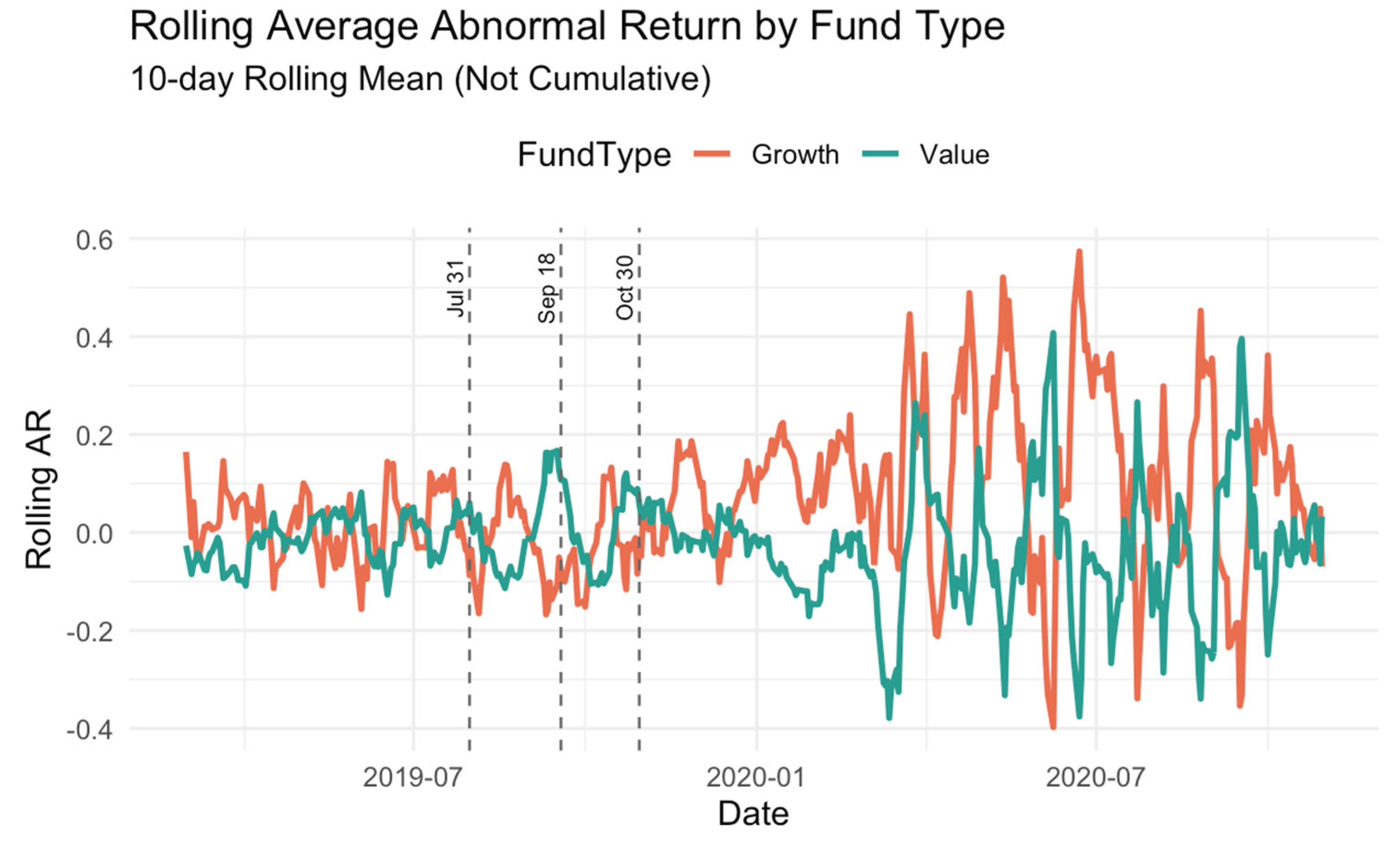
The event study framework can identify differences in fund performance that cannot be explained by general market volatility. We calculate the AR relative to the expected return of a CAPM-based benchmark model for each defined event window. Appendix C Figure A3 shows the 10-day rolling average AR of growth and value mutual funds. Growth funds exhibit higher positive AR after 2020, indicating that value funds are more market-responsive than growth funds.
To measure the aggregate impact of policy announcements, we construct CARs for the three event windows surrounding the Fed’s rate cut. We use static β coefficients estimated based on full-sample regressions, especially for short-term event windows. This is because rolling estimates are noisy over a short period of time. We use rolling β better to identify time-varying market risk exposures over the long-term window. To test the benchmark, we also create a pre-interest rate cut window (July 1st -31st) and a non-event period that covers all dates except the event window. We consider the 30 days before the rate cut as a sub-window of the broader event window, i.e., the 30 days before the Fed decides to cut rates. In contrast to the non-event period, this window covers all time frames outside the defined event window. ANOVA and t-tests are then used to compare CARs across styles and periods, and to distinguish between differential effects. In addition, we combine ordinary least squares (OLS) regressions that incorporate style and period interactions. We estimate a pooled OLS model of CAR based on fund style, cycle indicators, and their interactions:
Where is CAR of the ith fund on day t within the ±30-day window; is a dummy variable for value funds (Value=1, Growth=0); and are indicator variables for non-event and event windows, respectively (Pre-Cut is the benchmark); measures the marginal difference of value funds relative to growth funds in each period.
To explore whether growth and value funds react differently to each rate cut, we estimate separate cross-sectional regressions of 30-day CAR on fund style for each event date :
Where if fund i is value (0 if Growth).
To assess the persistence of the impact of monetary policy, we use dynamic AR with rolling β to calculate CARs for two long-term maturities following the October 30, 2019, rate cut: 6 months (as of April 30, 2020) and 1 year (as of October 30, 2020). Since events 1 and 2 occur after other policy adjustments, the long-run CAR may be disturbed. Therefore, the long-run regression analysis does not include the long-run CAR. For each horizon , we estimate the cross-sectional model:
Where if fund i is value (0 if Growth).
Heteroskedasticity-consistent covariance matrix estimator, type 1 (HC1), for robustness checks, is used in all models. We perform a studentized Breusch-Pagan (BP) test (p < 0.001) on each model to validate heteroskedasticity. Therefore, the reported coefficients are all estimates under robust standard errors (SE).
We construct the following cross-sectional regression model to assess the difference in performance between growth and value funds after excluding market risk.
are the 30-day CARs obtained by accumulating the CAPM ARs. is the fund style indicator variable, which is taken as 1 for growth and 0 for value; can be taken in two ways: For the static β, which is CAPM β from a one-time regression of the full sample, another, the rolling β used CAPM regression with a rolling window of 30 or 60 days in the past to extract day-by-day β. Also, we do the robustness check with the HC1 method.
To test whether the style effect varies with a fund’s market sensitivity, we estimate cross-sectional interaction models of the following form:
Where is the 30-day CAR for fund i (static event windows). ∈ {0,1} equals 1 for Growth funds, 0 for Value. is the fund’s systematic risk exposure, measured both as Static CAPM beta over the full sample, and 30-day rolling CAPM beta, estimated via OLS in a moving window. The interaction term captures whether the style effect (growth vs. value) changes with market sensitivity. All models employ HC1-robust SEs to address heteroskedasticity, as confirmed by studentized BP tests.
3.4. Capital Asset Pricing Model
This study uses the CAPM as the underlying risk-adjustment framework to differentiate the impact of market-wide risk factors on fund performance. The CAPM assumes that the expected return of an asset is a linear function of its sensitivity to systematic market risk and is expressed as follows.
Where is the expected return on asset i, is the risk-free rate, is the asset’s beta, and the is the expected return on the market portfolio [29].
In empirical applications, the CAPM framework provides a benchmark for measuring fund performance after adjusting for market risk exposure. The framework allows for rigorous tests of performance metrics to distinguish returns attributable to skill from those attributable to market changes [30]. A fund’s alpha, representing the excess return over its beta-implied benchmark, serves as a measure of a fund manager’s ability or pricing efficiency [15].
3.5. Risk-Adjusted Performance: Sharpe Ratio and Jensen’s Alpha
Risk-adjusted performance metrics allow for differences in volatility and market risk to be accounted for in performance comparisons. The SR and a are two common metrics. Sharpe [14] proposed the SR to calculate the excess return per unit of risky investment. Its expression is:
Where is the fund’s average return, is the risk-free rate, and is the standard deviation (SD) of returns. The SR shows how well a fund compensates investors for their total risk (including systematic and idiosyncratic risk).
By contrast, a assesses the AR for exposure to systematic risk and is derived from the CAPM framework.
Where is a of asset, is realized return of asset, is risk-free rate, is beta of asset, and is realized return of the market.
A positive alpha indicates that a fund outperforms its risk-adjusted benchmark, implying that the fund manager has good exposure or superior management skills over the sample period [15]. By integrating these two metrics, we can get a more complete picture of mutual fund performance. a evaluates whether returns are commensurate with market risk, and the SR measures risk-return efficiency. Both methods are particularly important during periods of monetary easing, when volatility and investor sentiment can fluctuate rapidly.
3.6. Rolling Performance Measures and Time-Varying Risk
Traditional performance assessment typically assumes constant risk exposure and constant return distribution. However, financial markets can exhibit abnormal volatility, heteroskedasticity, and changes in investor behavior when macroeconomic events such as interest rate changes occur [31]. This study uses rolling window techniques of the SR, a, and β to capture these dynamics. Specifically:
The rolling SR expression is:
Where and are the mean and SD of returns over a rolling window up to time t.
Additionally, Christopherson et al. [32] used rolling regression to identify changes in fund strategies. For the rolling a, the time-varying alpha can be represented by repeatedly estimating CAPM regression over rolling sub-periods, using the formula:
Where is the a of fund i at time t, represents the fund’s excess return adjusted for systematic risk. is fund’s i actual return at t, is risk-free rate of return at t, is the fund’s systematic exposure to the market estimated in the rolling window, is the actual return of the market at t; denotes the market risk premium.
Meanwhile, rolling β coefficients are analogous to rolling CAPM regressions to reflect changing market risk exposures. Ferson and Schadt [33] introduced the methodology of time-varying β coefficients to assess conditional performance. Repeated regressions are conducted over a rolling window to estimate the sensitivity of each fund’s returns to changes in market returns. The expression is:
Where is the real rate of return earned by the fund p in time t, is the profitability of the market at time t, is the risk-free rate of return, usually using the current short-term Treasury rate. is denotes systematic risk exposure and excess market returns. is the rolling β coefficient at time t, which shows the fund’s dynamic sensitivity to market changes, is the rolling intercept term, which indicates the trend of excess return over the time window, and is the error term, which captures the unexplained part of the model.
By using rolling calculations over a 30-day window, this study provides a more detailed understanding of how fund risk and performance evolve in response to policy changes. Rolling calculations can better reveal risk exposure or short-term performance fluctuations than static metrics, which may miss or ignore these factors entirely.
Therefore, this study uses rolling alphas and SRs to demonstrate the emergence and dissipation of the performance advantage of growth funds versus value funds under different monetary policy regimes. In addition, this is consistent with more econometric approaches that identify time-varying parametric models and conditional risk. This dynamic approach can also reveal whether, when, and how monetary easing affects fund returns and volatility.
3.7. Data Sources and Sample Selection
This study focuses on three consecutive rate cuts implemented by the Fed between March 2019 and October 2020 (July 31, September 18, and October 30, 2019). This time frame was chosen for four main reasons: (1) availability of high-frequency, high-quality mutual fund data suitable for both static and rolling measurements; (2) simplicity of a common easing cycle, which is separable from interventions triggered by crises; (3) occurrence at a time preceding extensive unconventional policies like quantitative easing, thus making it ideal for identifying rate cuts effects; (4) the presence of multiple, clustered events allows for robust event study design across repeated windows.
To assess the impact of the Fed’s rate cut on mutual fund performance, we select six well-known equity mutual funds and categorize them into growth and value funds. The growth funds include Vanguard Growth Index Fund Admiral Shares (VIGAX), Fidelity Growth Company Fund (FDGRX), and T. Rowe Price Blue Chip Growth Fund (TRBCX). These funds are more sensitive to economic stimulus measures such as interest rate cuts because of their emphasis on high expected earnings growth and large-cap allocations. In contrast, value funds include the Vanguard Value Index Fund Admiral Shares (VVIAX), Dodge & Cox Stock Fund (DODGX), and American Funds Washington Mutual Investors Fund (AWSHX). These funds focus on fundamentally driven pricing, stable dividends, and low valuations, and are therefore less sensitive to monetary policy shocks.
Daily adjusted closing prices and return series for all funds are obtained from Seeking Alpha [34] with fund returns calculated using the log difference of adjusted prices to account for dividends and stock splits. For more information, see Table 1.
Furthermore, we use the Chicago Board Options Exchange (CBOE) Volatility Index (VIX) and the Standard & Poor’s 500 Index (SPX) as benchmarks to account for the overall market impact, sourced from Seeking Alpha [34], which helps contextualize mutual fund behavior within broader market dynamics. For trends in the benchmarks (SPX and VIX) during the study period, please refer to Appendix C Figure A1, which illustrates that SPX remained relatively stable throughout the event window, while VIX was volatile thereafter, during the onset of the COVID-19 pandemic.
While NASDAQ [35] provides broader market indicators, we use the Federal funds rate (FFUNDS) to represent the monetary policy stance. Unlike stock prices, FFUNDS does not exhibit daily percentage changes, as it reflects a fixed-income rate that adjusts infrequently. Studies analyzing the impact of interest rates on asset prices use first-order differences (∆ FFUNDS) rather than percentage returns [3]. Our study computes first-order differences of FFUNDS to track monetary policy shifts. We calculate the required risk-free rate within a CAPM framework using the FRED database of 3-month Treasury Bill rates (TB3MS) [36]. To ensure the continuity of the sample data, the monthly TB3MS series is populated using the last observation carried forward (LOCF) and linearly interpolated to daily frequencies. The final decimalized daily series is used for all risk-adjusted performance estimates.
This sample construction ensures that the funds selected are indexed, actively managed, or liquid, and fit each investment style. To ensure representativeness, comparability, and analytical robustness based on the event-based and risk-adjusted return analysis, the sample is designed using a balanced mix of fund styles, validated sources, and composite market benchmarks.
3.8. Time Window Definition
To systematically evaluate the impact of interest rate cuts on mutual fund performance, this study adopts a multi-perspective event study framework. This study defines both short-term and long-term windows to capture the immediate effects and persistent adjustments of monetary policy shocks across distinct fund styles. In addition, exploring these windows provides a clear understanding of whether the market reactions are concentrated around the announcement date or evolve gradually over time.
This study examines short-term impacts using symmetric event windows centered on each of the 2019 Fed rate cut announcements: July 31st, September 18th, and October 30th. For each event, we construct a window spanning [-30, +30] trading days around the event date.
For the short-term analysis, three symmetric event windows are constructed around the Fed’s 2019 rate cut announcements on July 31, September 18, and October 30, each spanning ±30 trading days. These windows capture pre-announcement anticipation and immediate post-announcement adjustments, aligning with standard event study methodology [28]. AR and CAR are computed within these windows to quantify the direct valuation effects of rate cuts.
To explore the long-term effects, two extended post-event windows are defined using the final rate cut on October 30, 2019, as the anchor point: one from October 30, 2019 to April 30, 2020 (6 months), and another from October 30, 2019 to October 30, 2020 (1 year). These windows allow for analysis of performance persistence, particularly in terms of risk-adjusted measures such as SR and a. This approach also facilitates a comparison between short-term market reactions and long-term absorption of monetary easing, offering insights into the durability of style-specific fund performance.
This window structure allows for broader economic correlation and event-specific granularity. Long-term windows are used to examine variations in fund response patterns, while short-term windows are used to limit announcement effects. The use of multiple overlapping and non-overlapping windows enhances the reliability and credibility of empirical inferences.
3.9. Variable Construction
To put into practice the theoretical concepts and empirical models presented in the previous chapters, this study constructs a comprehensive set of variables to capture fund-level performance, risk exposure, and policy response dynamics. These variables are designed to support both event-based and risk-adjusted analysis.
The logarithmic difference of daily returns is calculated for each mutual fund after adjustment. Expected returns are derived using both static and dynamic approaches based on the CAPM framework. Static estimates are based on the full sample β coefficients, while dynamic estimates are based on 30-day rolling window regressions. These techniques enable time-varying estimates of β, alpha, and AR that adapt to changes in fund behavior and risk exposure over the policy cycle.
SRs and α are computed on a static and rolling basis, respectively, to quantify risk-adjusted performance. The SR on a 30-day rolling basis applies realized 30-day return volatility, and the rolling alpha is the intercept from a rolling CAPM regression. These rolling structures can be used for performance sensitivity analysis in a changing market environment. Event-related variables consist of multiple window dummies, each indicating whether the date is pre-event, post-event, or within the window. These factors allow for a direct assessment of the short-term and long-term impact of policies on fund outcomes.
Each variable is constructed using the R programming language. A complete dictionary of all 38 dataset variables, including the internal processing steps and code-based construction logic, can be found in the full list of variables and definitions in Appendix A Table A1, while the key variable definitions in Table 2 provide a summary of the core variables and their mathematical definitions.
3.10. Risk-Adjusted Performance Analysis
This study uses risk-adjusted metrics to assess the performance of mutual funds to complement the analysis of ARs. The SR measures average excess return per unit of total risk (SD), which is particularly sensitive to changes in volatility associated with policy events. In addition, a is derived from the CAPM framework, which separates the portion of a fund’s return that cannot be explained by market volatility and indicates the ability or strategic advantage of the fund manager in the event of a change in monetary policy. The expression is shown in Table 2.
At the fund level, both metrics are estimated using two approaches: static estimation, which averages performance over the entire sample period, and rolling estimation using a 30-day moving window to observe changes in policy interventions. The rolling methodology is particularly well-suited to capturing short-term increases or decreases in performance associated with policy changes or macroeconomic uncertainty. These rolling statistics are calculated using consistent window lengths and are consistent across all funds and dates.
We summarize the results for growth and value funds separately to assess the differences between investment styles. Subsequently, the results section presents rolling estimates of the SR and a. In addition, descriptive statistics are used to summarize their distributions. The use of these dynamic indicators allows us to assess whether monetary easing has been of great benefit to growth funds in terms of risk-adjusted returns.
3.10.1. Sharpe Ratio Regression Framework
Using static and rolling SRs as dependent variables, this study estimates a set of structured linear regression models to determine whether there is a systematic difference in the risk-adjusted performance of growth and value funds, particularly in respect to monetary policy intervention. Table 3 summarizes the modeling framework and outlines the use of each model.
The first is the cross-sectional model (S1), which uses static SRs computed on the entire sample for baseline comparisons. After adjusting for return volatility, it confirms that growth funds outperform value funds.
Model S4 uses a rolling 30-day SR, regressed on fund style, to capture the dynamics of performance over time. This formula can document the change in risk-return efficiency of different types of funds during and after the policy adjustment period. Models S4_w1 to S4_w5 replicate rolling Sharpe regressions within a discrete event window. These windows include six months and one year after the event, as well as three short-term windows before and after each rate cut. These regressions indicate whether the advantage of growth funds strengthens or weakens during each monetary event.
The core model S5 introduces dummy variables for three time periods (pre-cuts, non-events, and events) and relates them to fund style. This identifies how growth and value funds perform in different monetary environments and provides key evidence of the cyclical sensitivity of fund styles.
Model S6 adds rolling volatility and contemporaneous indicators of market returns to control for other drivers of fund performance. This helps to differentiate between style effects by moderating short-term noise and macro risk.
Finally, model S8_interact analyzes the more complex relationship between style and rolling market returns. How do growth funds perform when the market is trending upward? This reflects the duration-based valuation theory in an environment of monetary easing. Interpretation of the results is based on economic magnitude and statistical significance, focusing on the style coefficients and key interaction terms across time partitions.
3.10.2. Jensen’s Alpha Regression Framework
This study constructs a series of a regression models based on the CAPM framework to assess the impact of monetary policy on risk-adjusted performance. These models use time series and panel structures to compute static and rolling a value for growth and value funds. Furthermore, they incorporate multiple control variables and interaction terms.
The analysis begins with a benchmark model (model lm_model2 in Table 4), which compares the average a of the various fund styles. This serves as a benchmark for CAPM-based differences in style performance. To provide a dynamic view of style-sensitive risk-adjusted performance, we calculate rolling alpha over a 30-day window (lm_model4) to account for time variation.
By introducing a market return control variable (lm_model3) and an interaction term between fund style and excess market returns (lm_model3_interact), the subsequent model allows for the assessment of heterogeneous responses to market volatility. We add rolling volatility as a control variable (lm_model6) and interact it with fund style to assess the sensitivity to style-related volatility shocks (lm_model6_interact). This further accounts for risk conditions.
Furthermore, we use an event window interaction model (lm_model12_interact) to analyze the impact of policies at specific points in time. The model estimates whether the Jensen alpha changes within a discrete window centered around each rate cut. Finally, a cycle-level interaction model called lm_model14 analyzes alpha performance under a broader set of regimes (pre-cuts, non-event periods, and event periods) to identify differences in style conditional on the stage of monetary policy.
Table 4 contains all model specifications, variable structures, and estimation purposes. This structured framework allows for comparing a dynamics across different market and policy environments.
4. Results
4.1. CAR Results
4.1.1. Car Results Across Event Windows
Growth funds generally outperform value funds. Table 5 summarizes the SD and average CARs of growth and value funds across the three key event windows. Across all event windows (± 30 days, 6 months, and 1 year), growth funds consistently and significantly outperform value funds, both in raw CAR and in interaction regression estimates. Detailed CAR statistics are provided in Appendix B Table A2, with full cross-window profiles illustrated in Appendix C Figure C2.
To assess the difference in CAR between growth and value funds across different event windows (short-term and long-term), we use independent samples t-tests. Levene’s chi-square test reveals that the assumption of equal variance is not met for most of the windows, except for Event 1 and the pre-interest rate cut period (see Appendix B Table A3). Therefore, Welch t-tests are used under appropriate conditions (p-values below 0.05).
Table 6 shows that growth funds consistently outperform value funds across all event windows. It is noteworthy that in the year following the rate cut in October 2019, the CAR of growth funds averaged 14.64% and that of value funds averaged 5.31% (t=41.39, p<0.001), indicating a sustained and significant advantage for growth funds. The short-term (±30 days) CAR difference between growth and value funds is also significant (t = 15.92, p < 0.001), further confirming the immediate advantage of growth strategies. These findings suggest that monetary policy shocks, especially interest rate cuts, typically benefit growth funds more than value funds. For more information, see Appendix B Table A4.
To compare performance across different periods, we classify CAR observations into event, pre-cut, and non-event windows. Appendix B Table A5 summarizes the descriptive statistics of CAR across different periods. Welch’s ANOVA confirms significant differences between group means (F = 110.25, df = 2, p = 0.001). Levene’s test indicates heteroskedasticity (p = 0.001). Post-hoc Games-Howell tests reveal that CARs during the event window were significantly lower than those in the pre-cut and non-event periods (both p < 0.001). Full results are in Appendix B Table A6.
Regression results reinforce the theoretical view that growth funds, due to their long-duration cash flows, are more sensitive to interest rate cuts. Significant interaction terms (e.g., value × event) confirm this asymmetric response. Table 7 shows the estimated coefficient errors for the HC1 robust standard (Robust SE). Justifying the robust SE correction, the student’s BP test strongly rejects homoskedasticity (BP = 418.27, p < 0.001). The event dummy variable is positive and highly significant (β3 = 7.898, p < 0.001), indicating that growth funds (omitted styles) are approximately 7.9 percentage points higher CAR than that of growth funds during the 30-day window after the rate cut. Growth funds underperform value funds by 10.8 percentage points in the event window, with a negative and highly significant value x event interaction (β5= -10.820, p<0.001). The difference in styles is insignificant before and during non-interest rate cuts (β1 and β4).
The observed pattern is like the asset pricing logic: interest rate cuts reduce the discount rate of future cash flows, and growth stocks are more dependent on long-term returns [10]. In addition, the sensitivity of growth stocks to changes in interest rates increases as their future cash flows increase [37]. The CAR of growth funds exceeds their market-adjusted return, suggesting that their outperformance is not solely attributable to systematic risk exposure.
In addition, the results reflect behavioral responses; in fact, interest rate cuts not only reduce borrowing costs but also increase investors’ risk appetite. Furthermore, the behavioral reaction of investors may cause growth funds to overreact. Behavioral finance focuses on how investor sentiment and style-based flows affect monetary policy. For example, “yield chasing” is a phenomenon that suggests that investors are more likely to shift funds to investment opportunities with high risk and high growth potential [38]. Such reallocation flows enable growth funds to outperform mechanical valuation effects.
4.1.2. Event-By-Event Regression Analysis
Table 8 presents the robust coefficient estimates and t-statistics: Growth funds significantly outperformed value funds following the July 31 and October 30 rate cuts (β = -1.525 and -1.400, respectively; both p < 0.001), while the pattern reversed on September 18 (β = +1.166, p < 0.001) with value funds earning higher ARs. These events suggest that the success of value and growth funds depends largely on the timing of the Fed intervention.
The persistent growth fund premium over the 6-month and 1-year windows suggests a structural shift in investor preferences following monetary easing. Notably, value funds briefly outperformed growth funds around the September 18 rate cut, likely because the cut had already been priced in by growth stocks. Meanwhile, value stocks may have attracted capital through a catch-up effect or flight to safety amid escalating trade tensions and recession fears. These dynamics underscore the importance of aligning monetary policy actions with prevailing market expectations to ensure effective transmission. To assess whether these performance gaps persist over longer horizons, we extend the analysis using 6-month and 1-year CAR regressions.
4.1.3. Long-Term Dynamic Car Analysis
We conduct a studentized BP test on the two regressions. The results show that BP = 33.656, p = 0.000 (<0.001) for the 6-month model and BP = 210.520, p = 0.000 (<0.001) for the 1-year model. Therefore, we report HC1 robust SEs for all coefficients. Appendix B Table A4 contains the heteroskedasticity test statistics and confidence intervals. Appendix B Table A7 contains the complete test statistics and regression results.
Table 9 shows that the average CAR of growth funds is 4.94% in the 6-month window, while that of value funds is 7.15 percentage points lower on average (p < 0.001). In the 1-year window, the average CAR for growth funds reaches 10.94%, again exceeding that of value funds by 15.04 percentage points (p < 0.001).
This suggests that the long-term impact of the Fed Board’s interest rate cuts is significantly different across fund styles, with growth funds consistently outperforming value funds over extended post-cut periods. The pronounced and sustained divergence in CAR between the 6-month and 1-year periods suggests that monetary easing influences not only short-term valuations but also long-term investment behavior. In low-interest-rate environments, both asset valuations and capital allocation tend to shift toward growth-oriented strategies [3]. This performance premium reflects both fundamental valuation sensitivity and sentiment-driven capital flows, highlighting the role of expectations and market context in shaping the transmission of monetary policy.
4.1.4. Regression Model of Style Effect and Systematic Risk
To assess whether the outperformance of growth funds is solely due to higher market exposure. Table 10 shows that growth funds significantly outperform value funds across all specifications, even after controlling for systematic market exposure (Beta). In the static model, the average CAR for growth funds exceeds that of value funds by 2.04 percentage points (γ = 0.020, p = 0.005). This premium becomes more pronounced in the 30-day and 60-day rolling Beta models, rising to 19.34% and 14.0%, respectively (both p < 0.001). These results confirm that the observed style premium is not merely driven by differences in Beta exposure.
We estimate interaction models using static and 30-day rolling beta coefficients to determine whether market exposure affects the relationship between fund style and CAR. Table 11 shows the regression estimates based on HC1. Full results are provided in Appendix B Table A8 and Table A9.
In the static Beta model, the coefficient of the interaction term between the growth dummy variable and Beta (θ = 0.035, t = 17.96, p < 0.001) indicates that the performance advantage of growth funds over value funds increases with market Beta. In other words, during periods of monetary easing, when market exposure is greater, the return premium for growth strategies is higher.
In the rolling Beta model, the interaction term is negative and significant (θ = -0.008, p < 0.001), indicating that the growth premium declines as Beta increases. This likely reflects heightened downside risk or volatility in high-Beta growth funds during turbulent periods following rate cuts. Both specifications suggest that the growth premium is dynamic and varies systematically with the fund’s market exposure. These results suggest that controlling for time-varying and static β coefficients is crucial in assessing abnormal performance after monetary policy interventions.
4.2. Risk-Adjusted Performance Results
4.2.1. Dynamic Sharpe Ratio and Jensen Alpha Trend
Figure 1 and Figure 2 display the 30-day rolling SRs and a for growth and value mutual funds surrounding the three key Fed rate cuts in 2019 (July 31, September 18, and October 30). Dashed vertical lines denote the announcement dates (mark the three interest rate cuts announced by the Fed in 2019).
Both fund types show fluctuations in performance metrics over the observation period. However, growth funds consistently improve in risk-adjusted returns after each rate cut. Their Sharpe Ratio increased significantly after October 2019. This indicates that they offer a higher excess return for each unit of risk in response to monetary easing. Rolling CAPM regressions indicate that growth funds have higher and more volatile α estimates than value funds. After October, growth fund α values occasionally exceed 0.4, showing better performance relative to systematic risk. These patterns support the idea that growth-oriented assets, because of their longer duration, are more affected by interest rate cuts.
4.2.2. Sharpe Ratio Regression Results
To assess the risk-adjusted performance difference between growth and value funds under monetary easing, we estimate a series of SR regressions. Table 12 reports both static (S1) and rolling (S4) specifications. In both models, the negative coefficient on the growth dummy indicates that growth funds exhibit consistently higher SRs than value funds. This difference becomes more pronounced in the rolling model (γ = – 0.0887, p < 0.001).
Table 13 further decomposes the rolling model (S4) by event window. The performance gap is small in the pre-cut and initial event windows, but widens significantly post-October 30, with the growth premium reaching approximately -0.10 in both the 6-month and 1-year windows. This temporal pattern supports the hypothesis that growth funds benefit more under prolonged easing conditions.
Table 14 introduces an interaction model (S5) using policy period indicators. The “growth × event” term is statistically significant (γ = - 0.0398, p < 0.001), while “growth × non-event” is insignificant, reinforcing the view that the growth premium is concentrated in easing windows rather than constant across time.
Table 15 presents model S6, which controls for market excess returns and 30-day rolling volatility. Growth funds consistently deliver favorable risk-adjusted returns regardless of the volatility of the underlying market. This demonstrates that the style effect remains statistically significant (γ = - 0.0870, p < 0.001) even after accounting for these control variables, confirming that growth funds remain statistically significant. The fact that the coefficients of both control variables are positive and highly significant further supports the importance of market conditions in driving the dynamics of the SR.
Table 16 (Model S8_interact) assesses whether growth funds are more responsive to market returns. The negative interaction coefficient (-0.1229, p < 0.001) suggests that growth fund Sharpe ratios increase less steeply with market gains, indicating convex risk-return behavior, consistent with the theoretical sensitivity of long-duration assets to changes in discount rates.
The results from the SR regression provide evidence that the Federal Reserve’s 2019 interest rate cuts had a very positive influence on the risk-adjusted performance of mutual funds, with growth-based funds exhibiting the most substantial response. Growth funds showed a consistent SR premium over value funds, especially across long-term windows, indicating that the effects of monetary easing are sustained rather than short-lived.
The regression coefficients on the value fund dummy were consistently negative, corroborating valuation theory due to the sensitivity of assets with cash flows at longer durations, such as growth stocks, to falling discount rates. The significant interaction term between growth style and event periods underscores that this performance divergence is policy-driven rather than coincidental.
Moreover, robustness checks incorporating rolling volatility and market returns show that the observed style effect is not simply a reflection of broader market dynamics. Growth funds exhibit pro-cyclical behavior, amplifying gains in bullish markets and showing heightened sensitivity during downturns, reflecting a non-linear risk-return profile. Ultimately, it can be concluded that expansionary monetary policy enhances both the relative and absolute Sharpe performance of growth funds, reinforcing the strategic role of interest rate cycles in shaping style-based investment outcomes.
4.2.3. Results of Style Effects in Jensen’s Alpha
This section assesses risk-adjusted performance differences between growth and value funds using static, rolling, and interaction-enhanced CAPM α models. As shown in Table 17, growth fund dummies are consistently negative and highly significant across all specifications, indicating that growth funds generally underperform value funds on a risk-adjusted basis.
In the static model, the alpha for growth funds is 10.4 lower than for value funds (p < 0.001). This negative gap persists under 30-day rolling estimations and remains robust after controlling for rolling market excess returns and volatility (Table 17). Although controls slightly attenuate the effect, the performance disadvantage remains statistically and economically meaningful.
Interaction models provide further insights into how style differences vary with market dynamics and policy timing (Table 18). Growth funds’ alpha improves in rising markets (γ = -0.0923, p < 0.001) but deteriorates sharply as volatility increases (γ = -0.034, p < 0.001), reflecting their sensitivity to market uncertainty. Event-specific interactions reveal that growth funds performed significantly worse around the September 18 rate cut (γ = -0.137) but rebounded strongly after the October 30 cut (γ = 0.133), suggesting market timing and investor expectations played a critical role. Notably, alpha declines again over the one-year post-cut horizon (γ = -0.140), consistent with delayed transmission or valuation corrections.
At the cycle level, model lm_model14 confirms a pronounced negative alpha for growth funds during monetary easing periods (γ = - 0.081, p < 0.001), reinforcing the duration-based explanation for style dispersion during rate cut cycles.
The a regression results reveal that growth funds generally exhibit lower a returns than value funds, even after controlling for market returns and volatility. This aligns with theoretical expectations: growth funds, which depend more heavily on long-term cash flows, are structurally more sensitive to discount rate changes. The consistently negative style coefficients across both static and rolling models reflects this inherent vulnerability.
Interaction models further show that growth funds tend to outperform in bullish markets due to their pro-cyclical and speculative nature and underperform during periods of heightened volatility. This duality suggests that investors’ aversion to long-duration risk amplifies the sensitivity of growth portfolios during turbulent conditions.
Policy-window-specific regressions underscore that a effects are not uniform. While growth funds show positive a following the October 2019 rate cut, they underperform after the September cut, implying that market reactions depend on expectations, Fed communication tone, and broader macroeconomic narratives.
Overall, a regression findings highlight that monetary easing disproportionately affects growth fund performance, reinforcing the need for style-aware allocation and benchmark strategies under shifting policy regimes.
5. Summary
This research presents a systematic and multi-perspective examination of the effect of the U.S. Federal Reserve’s interest rate reductions throughout the 2019–2020 easing cycle on the performance of equity mutual funds with different investment styles. Using a combination of the event study approach, risk-adjusted performance measures, and regression-based estimation, we derive some important insights.
- Growth Fund Outperformance: Growth mutual funds consistently outperform value funds in both short-term and long-term windows, in terms of AR and risk-adjusted metrics (SR and α), reflecting their heightened sensitivity to changes in discount rate stemming from their longer-duration cash flow structures.
- Durability of the Growth Premium: The growth premium remains significant over both 6-month and 1-year windows, suggesting that monetary easing leads to persistent revaluation effects and sustained investor flows beyond short-term market reactions.
- Behavioral Amplification: Beyond valuation effects, investor behaviors such as increased risk appetite and style-based reallocations (such as yield chasing) further reinforce growth fund outperformance.
- Regression Validation of Style-Market Interaction: Regression models confirm that the growth premium persists after controlling market risk and volatility. The interaction effect reveals the growth funds’ pro-cyclicality, with elevated SR during market upturns and diminished performance during high volatility.
- Jensen Alpha Sensitivity: While growth funds exhibit lower average α due to their structural exposure to macro risk, they generate higher α in accommodative policy phases, though this edge is not always sustained over longer horizons.
The study has some limitations, pointing out the way for future refinement and extension. First, this analysis focuses on only six representative mutual stock funds: three growth funds and three value funds. The small sample size may limit the generalizability of the findings, even though these funds are carefully selected for their large asset bases, institutional reputations, and consistent investment styles. Although this “typical sample, in-depth analysis” approach is a best practice for event studies, a larger and more diversified fund sample would enhance external validity and cross-sectional robustness.
Second, the study focuses exclusively on the three major rate cuts in 2019, omitting rate hike episodes, fiscal stimulus, and other macroeconomic shocks. Therefore, the findings are only applicable to an easing cycle and may not generalize to tightening environments. Future research should examine asymmetric responses to interest rate hikes to capture the full sensitivity spectrum of fund styles.
Third, the long-term windows were inevitably included with the COVID-19 pandemic outbreak, introducing external volatility that may confound pure monetary policy effects. Such exogenous shocks may have amplified or confounded the policy impact, complicating explanations attributable only to changes in interest rates. Although this period offers a natural experiment on crisis-policy interaction, controlling for pandemic shocks, such as using dummies or excluding extreme months, could help to more clearly separate the effects of interest rates.
Fourth, the CAPM framework used in this study provides an easy-to-understand benchmark but neglects potentially influential style factors. Using multifactor models, such as Fama-French’s five-factor models, would improve explanatory power and contribute to a deeper understanding of performance attribution.
Finally, while this study focuses on official FOMC dates, the choice of event windows may still involve subjectivity. Incorporating market-based expectations to isolate “unexpected” monetary shocks could help distinguish between anticipated and surprise effects in future research.
Overall, future research could be extended to (1) increase the sample of mutual funds to cover more investment styles and strategies; (2) consider interest rate hike events to assess policy asymmetries; (3) use causal inference techniques, such as double-differencing or macro-control variables, to improve identification; (4) study multifactor models or quantile regressions to identify distributional effects; and (5) investigate fund responses under different monetary policy regimes. These extensions would enhance the theoretical depth and practical relevance of understanding mutual fund responses to monetary policy.
Supplementary Materials
The following supporting information can be downloaded at the website of this paper posted on Preprints.org. The supplementary datasets and replication code supporting this study are available on Zenodo at https://doi.org/10.5281/zenodo.17718728.
Author Contributions
Conceptualization, H.F. and M.S.; methodology, H.F.; software, H.F.; validation, H.F. and M.S.; formal analysis, H.F.; investigation, H.F.; resources, H.F.; data curation, H.F.; writing—original draft preparation, H.F.; writing—review and editing, H.F. and M.S.; visualization, H.F.; supervision, M.S.; project administration, H.F. and M.S.
Data Availability Statement
The processed dataset and replication code generated in this study are publicly available on Zenodo at https://doi.org/10.5281/zenodo.17718728. Raw mutual fund and benchmark price data were obtained from Seeking Alpha and Nasdaq, which do not permit redistribution of downloaded historical files; therefore, these data cannot be shared. Users can reproduce the data-cleaning workflow by downloading the same tickers from authorized sources and following the provided template script. The 3-month Treasury Bill (TB3MS) series used to construct the daily risk-free rate is publicly available from the Federal Reserve Economic Data (FRED) database and is included in the supplementary archive.
Conflicts of Interest
The authors declare no conflicts of interest. The funders had no role in the design of the study; in the collection, analyses, or interpretation of data; in the writing of the manuscript; or in the decision to publish the results.
Appendix A
This table provides a complete mapping between the above empirical methods and their implementation in the R environment.

Table A1.
Full Variable List and Definitions.
| Variable | Definition / Processing |
|---|---|
| Date | Trading date (YYYY-MM-DD). |
| Ticker | Fund identifier. |
| FundType | Style classification. |
| Adj_Close | Adjusted NAV on date t. |
| Change_Pct | Daily NAV change. |
| Rolling_Volatility | 30-day rolling SD of Change_Pct |
| Risk_Free_Rate | Risk-Free Rate. |
| Risk_Free_Rate_daily | Dailyized TB3MS rate (converted from annual to daily basis by dividing by number of trading days). |
| Market_Return | Daily return of SPX. |
| Rolling_Market_Return | 30-day rolling mean of Market_Return. |
| beta | . |
| Rolling_beta | . |
| Expected_Return_static | . |
| AR_static | Static AR: Change_Pct − Expected_Return_static. |
| Expected_Return_dynamic | . |
| AR_dynamic | Dynamic AR: Change_Pct − Expected_Return_dynamic. |
| Is_Event_Window | =1 if date t lies within any ±30-day event window (around July 31, Sept 18, or Oct 30, 2019), else 0. |
| CAR_static_precut | Cumulative AR over the 30 days immediately before the first cut (July 1–July 30, 2019). |
| CAR_static_nonevent | Cumulative AR over a fixed 30-day non-event baseline window (outside any ±30 event periods). |
| CAR_static_event1 | Cumulative AR in Window 1: July 31 ± 30 days. |
| CAR_static_event2 | Cumulative AR in Window 2: Sept 18 ± 30 days. |
| CAR_static_event3 | Cumulative AR in Window 3: Oct 30 ± 30 days. |
| CAR_dynamic_event3_6m | Cumulative AR_dynamic from Oct 30, 2019 to Apr 30, 2020 (6 months). |
| CAR_dynamic_event3_1y | Cumulative AR_dynamic from Oct 30, 2019 to Oct 30, 2020 (1 year). |
| Rolling_CAR | 30-day rolling sum of AR_static. |
| Rolling_AR | 10-day rolling mean of AR_static. |
| Period | Categorical factor: “Pre-Cut” / “Non-Event” / “Event”, based on “Is_Event_Window” and baseline periods. |
| GrowthDummy | Fund style dummy: 1 if Growth, 0 if Value. |
| Sharpe_Ratio | over full sample. |
| Rolling_Sharpe_Ratio | 30-day rolling SR, computed within each moving window. |
| Jensen_Alpha | : intercept from full-sample CAPM regression. |
| Rolling_Jensen_Alpha | : intercept from each 30-day CAPM regression. |
| D_Precut | =1 if t is within 30 days before first cut (July 1–July 30, 2019), else 0. |
| D_Window_1 | =1 if t falls in Window 1 (July 31 ± 30 days), else 0. |
| D_Window_2 | =1 if t falls in Window 2 (Sept 18 ± 30 days), else 0. |
| D_Window_3 | =1 if t falls in Window 3 (Oct 30 ± 30 days), else 0. |
| D_Long_6M | =1 if t is within 6 months after Oct 30, 2019, else 0. |
| D_Long_1Y | =1 if t is within 1 year after Oct 30, 2019, else 0. |
Appendix B
Table A2.
Full CAR Statistics by Window and Fund Style.
| Windows | Fund Type | Mean_CAR | SD_CAR | N |
|---|---|---|---|---|
| Pre-cut (30 days before cut) | Growth | 0.7686690 | 0.4372399 | 66 |
| Value | –0.3446675 | 0.3821128 | 66 | |
| Non-event (baseline 30 days) | Growth | 0.7530510 | 1.2140930 | 252 |
| Value | –1.1926922 | 1.0038934 | 252 | |
| Event 1 (±30 days around 7/31) | Growth | 0.8375585 | 0.6970253 | 132 |
| Value | –0.6349962 | 0.8021728 | 132 | |
| Event 2 (±30 days around 9/18) | Growth | –0.8994180 | 1.1778623 | 132 |
| Value | 0.4130666 | 0.7213801 | 132 | |
| Event 3 (±30 days around 10/30) | Growth | 1.0923349 | 1.3108540 | 132 |
| Value | –0.2784451 | 0.6599933 | 132 | |
| 6-month post-cut | Growth | 5.3559192 | 4.9445861 | 378 |
| Value | –2.3984893 | 3.9893903 | 378 | |
| 1-year post-cut | Growth | 14.6353598 | 11.4278271 | 762 |
| Value | –5.3066972 | 6.8051717 | 762 |
Note. N in the table is the total number of fund-date observations in each window; all CARs are calculated cumulatively based on the corresponding AR series.
Table A3.
Levene’s Test for Equality of Variances in CAR by Event Window.
| Windows | Levene’s F-statistic | p-value |
|---|---|---|
| Pre-cut (30 days before cut) | 1.885 | 0.172 |
| Non-event (baseline 30 days) | 10.536 | 0.000*** |
| Event 1 (±30 days around 7/31) | 1.371 | 0.243 |
| Event 2 (±30 days around 9/18) | 25.332 | 0.000*** |
| Event 3 (±30 days around 10/30) | 22.841 | 0.000*** |
| 6-month post-cut | 22.679 | 0.000*** |
| 1-year post-cut | 160.324 | 0.000*** |
Notes. In the rejection of the null hypothesis of variance chi-square, the p-value is less than 0.05. p-value reported to three decimal places (values < 0.001 shown as 0.000). Significance: * p<0.10; ** p<0.05; *** p<0.01. For these windows, we used the Welch t-test for subsequent mean comparisons. Pre-cut and Event 1 are variance-aligned (p≥0.05), studentized t-test criteria.
Table A4.
Full Growth vs. Value Funds CAR T-test Result.
| Event Window | Growth Mean CAR (%) | Value Mean CAR (%) | t-statistic | p-value | 95% CI for Difference | Variance equal |
|---|---|---|---|---|---|---|
| Pre-cut (30 days before cut) | 0.769 | –0.345 | 15.576 | 0.000*** | [0.9719, 1.2547] | TRUE |
| Non-event (baseline 30 days) | 0.753 | –1.193 | 19.607 | 0.000*** | [1.7508, 2.1407] | FALSE |
| Event 1 (±30 days around 7/31) | 0.838 | –0.635 | 15.920 | 0.000*** | [1.2904, 1.6547] | TRUE |
| Event 2 (±30 days around 9/18) | –0.899 | 0.413 | –10.917 | 0.000*** | [–1.5494, –1.0755] | FALSE |
| Event 3 (±30 days around 10/30) | 1.092 | –0.278 | 10.731 | 0.000*** | [1.1188, 1.6227] | FALSE |
| 6-month post-cut | 5.356 | –2.398 | 23.730 | 0.000*** | [7.1129, 8.3960] | FALSE |
| 1-year post-cut | 14.635 | –5.307 | 41.388 | 0.000*** | [18.9968, 20.8873] | FALSE |
Note. Interpretation of p-values refers to Table A3. Within a given window, all means are CAR. Two-sample t-tests (= FALSE) and studentized’s t-tests (var_equal = TRUE) provide t-statistics and p-values based on Levine’s Variance Homogeneity test. The 95% confidence interval represents the difference (growth-value).
Table A5.
Summary Statistics of CAR by Period.
| Period | Mean CAR (%) | SD of CAR (%) | N |
|---|---|---|---|
| Event | 2.700 | 10.308 | 3,072 |
| Non-Event | –0.220 | 1.479 | 504 |
| Pre-Cut | 0.212 | 0.692 | 132 |
Notes. “Mean CAR” and “SD of CAR” are expressed in percentage points. N refers to the total number of fund-day observations in each period. On average, CAR during the event windows was significantly higher (Mean = 2.70, SD = 10.31, N = 3072), compared to both pre-cut (Mean = 0.21) and non-event periods (Mean = -0.22).
Table A6.
Pairwise Games–Howell CAR Comparisons by Event Window.
| Comparison | Estimate | 95% CI | p-value |
|---|---|---|---|
| CAR Event vs Non-Event | –2.920 | [–3.383, –2.458] | 0.000*** |
| CAR Event vs Pre-Cut | –2.489 | [–2.947, –2.030] | 0.000*** |
| CAR Non-Event vs Pre-Cut | 0.432 | [ 0.222, 0.642] | 0.000*** |
Note. Interpretation of p-values refers to Table A3.
Table A7.
Long-Term Dynamic CAR Regression and Heteroskedasticity Tests.
| Window | BP F-statistic | BP p-value | Intercept Estimate | Robust SE | t-statistic | p-value | Value vs. Growth Estimate | Robust SE | t-statistic | p-value |
|---|---|---|---|---|---|---|---|---|---|---|
| 6-Month Post-Cut | 33.656 | 0.000*** | 4.943 | 0.172 | 28.662 | 0.000 | –7.146 | 0.219 | –32.593 | 0.000*** |
| 1-Year Post-Cut | 210.520 | 0.000*** | 10.938 | 0.309 | 35.440 | 0.000 | –15.040 | 0.355 | –42.383 | 0.000*** |
Notes. BP = studentized BP F-statistic (df = 1); BP p-value reported to three decimals (<0.001 shown as 0.000). Intercept = mean CAR for Growth funds; Value vs. Growth = difference in mean CAR (Value – Growth). Interpretation of p-values refers to Table A3.
Table A8.
Interaction of CAR with Static CAPM Beta.
| Term | Estimate | Robust SE | t-statistic | p-value |
|---|---|---|---|---|
| (Intercept) | 0.9814 | 0.0023 | 421.179 | 0.000*** |
| Growth Dummy | 0.0107 | 0.0024 | 4.520 | 0.000*** |
| CAPM Beta | –0.0282 | 0.0019 | –14.830 | 0.000*** |
| Growth × CAPM Beta | 0.0345 | 0.0019 | 17.960 | 0.000*** |
Notes. Dependent variable: 30-day CAR in static event windows. Interpretation of p-values refers to Table A3.
Table A9.
Interaction of CAR with 30-Day Rolling Beta.
| Term | Estimate | Robust SE | t-statistic | p-value |
|---|---|---|---|---|
| (Intercept) | 0.9799 | 0.0012 | 801.433 | 0.000*** |
| Growth Dummy | 0.2301 | 0.0021 | 108.904 | 0.000*** |
| Rolling β | –0.0087 | 0.0002 | –57.267 | 0.000*** |
| Growth × Rolling β | –0.0084 | 0.0002 | –35.470 | 0.000*** |
Notes. Dependent variable: 30-day CAR computed with rolling β ARs. Interpretation of p-values refers to Table A3.
Appendix C
Figure A1, the SPX series uses its actual index values, while the VIX is displayed on a secondary axis to show its original scale. The shaded area represents the portfolio event window from June 30 to November 30, 2019. Vertical lines mark the Fed’s rate cut dates. SPX reflects overall market performance, while VIX measures expected market volatility, which increases during times of uncertainty. The sharp rise in VIX after the initial cuts presents market disruptions unrelated to monetary policy, such as the start of the COVID-19 pandemic.
Figure A1.
SPX and VIX trends surrounding the 2019 Fed rate cut events.
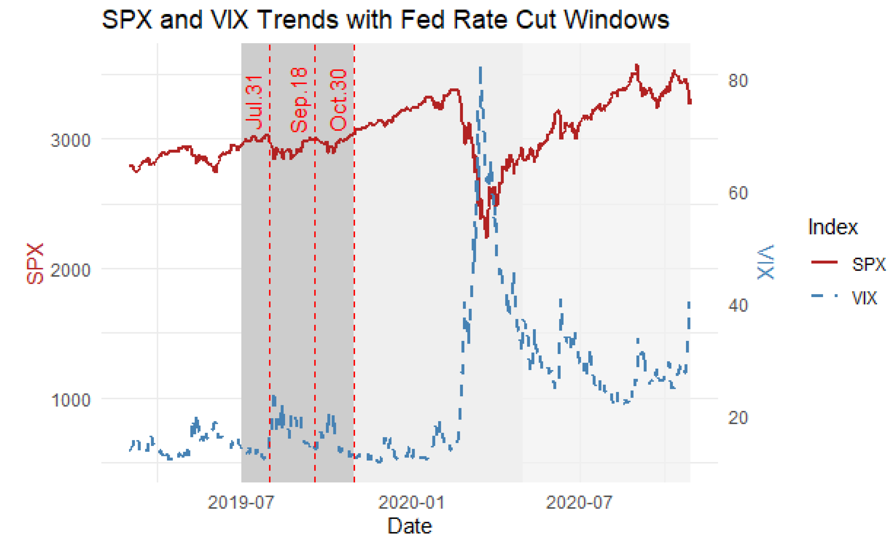
Figure A2 shows the average capital adequacy of value and growth funds over different event windows, including the control period and the three rate cuts. The event window is the major Fed rate cuts. Growth funds have significantly higher CARs in both the short- and long-term periods, while value funds typically have lower or negative ARs, especially during non-event periods.
Figure A2.
Mean CAR by Fund Type Across Event Windows.
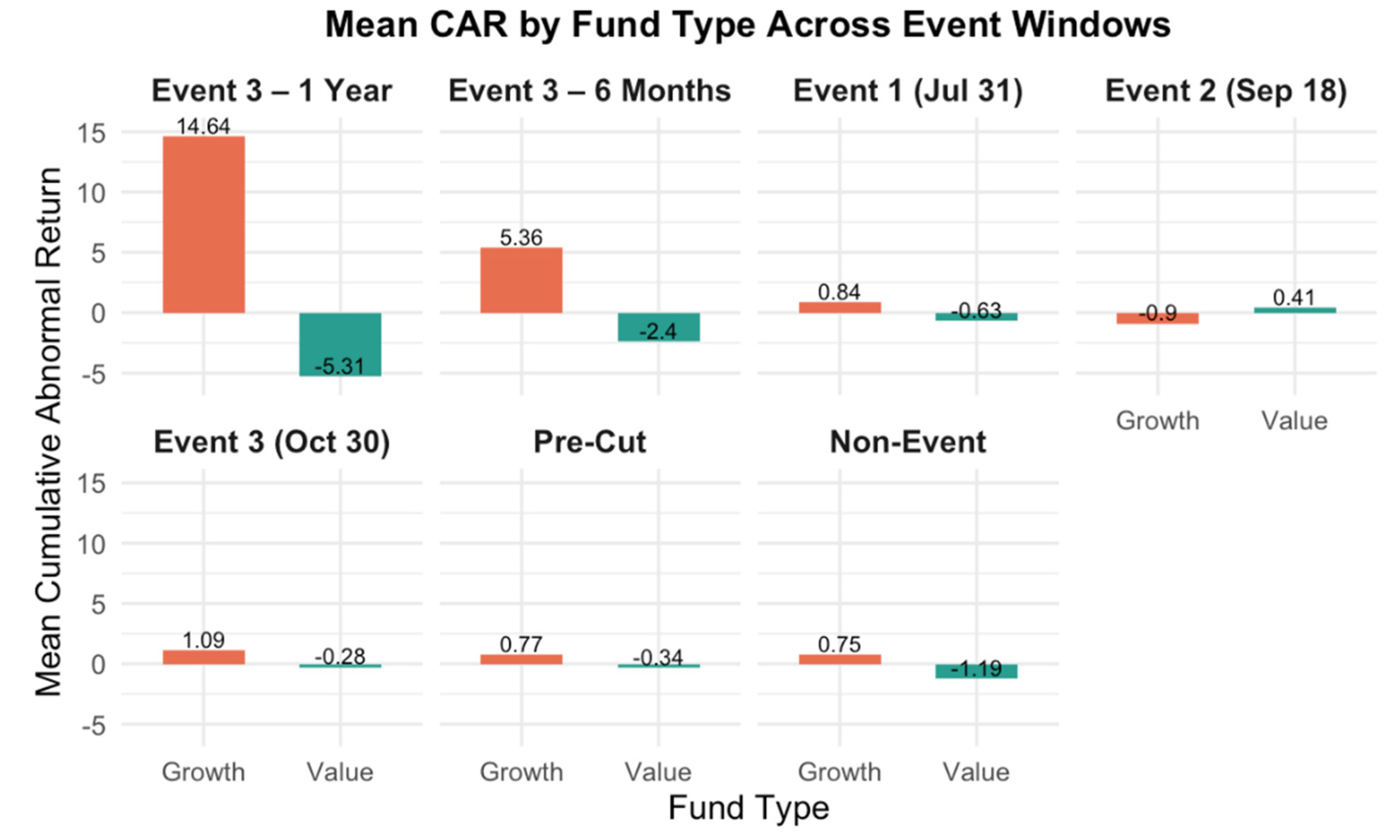
Figure A3, When the Fed cuts interest rates, the vertical dashed line represents this event.
Figure A3.
Rolling Average Abnormal Return by Fund Type.
References
- Bernanke, B.; Blinder, A. Credit, Money, and Aggregate Demand; National Bureau of Economic Research: Cambridge, MA, 1988; p. w2534. 2534.
- Taylor, J.B. Discretion versus Policy Rules in Practice. Carnegie-Rochester Conference Series on Public Policy 1993, 39, 195–214. [Google Scholar] [CrossRef]
- Bernanke, B.S.; Kuttner, K.N. What Explains the Stock Market’s Reaction to Federal Reserve Policy? The Journal of Finance 2005, 60, 1221–1257. [Google Scholar] [CrossRef]
- Estep, P.W. The Price/Earnings Ratio, Growth, and Interest Rates: The Smartest BET. JPM 2019, 45, 139–147. [Google Scholar] [CrossRef]
- Wachter, J.A.; Lettau, M. Why Is Long-Horizon Equity Less Risky? A Duration-Based Explanation of the Value Premium; National Bureau of Economic Research, 2005.
- Guo, H. Stock Prices, Firm Size, and Changes in the Federal Funds Rate Target. SSRN Journal 2002. [CrossRef]
- Jayawickrema, V. The Impact of Federal Reserve’s Conventional and Unconventional Monetary Policies on Equity Prices; Munich Personal RePEc Archive, 2020.
- Hojat, S.; Sharifzadeh, M. The Impact of Monetary Policy on the Equity Market. IJAMT 2017, 16. [Google Scholar] [CrossRef]
- Christian, W.; Woltering, R.-O.; Sebastian, S.P. The Interest Rate Sensitivity of Value and Growth Stocks – Evidence from Listed Real Estate.; Delft, The Netherlands, 2017.
- Fama, E.F.; French, K.R. Common Risk Factors in the Returns on Stocks and Bonds. Journal of Financial Economics 1993, 33, 3–56. [Google Scholar] [CrossRef]
- Fama, E.F.; French, K.R. A Five-Factor Asset Pricing Model. Journal of Financial Economics 2015, 116, 1–22. [Google Scholar] [CrossRef]
- Elton, E.J.; Gruber, M.J.; Blake, C.R. The Persistence of Risk-Adjusted Mutual Fund Performance. J BUS 1996, 69, 133. [Google Scholar] [CrossRef]
- Hammouda, A.; Saeed, A.; Vidal, M.; Vidal-García, J. On the Short-Term Persistence of Mutual Fund Performance in Europe. Research in International Business and Finance 2023, 65, 101963. [Google Scholar] [CrossRef]
- Sharpe, W.F. Mutual Fund Performance. J BUS 1966, 39, 119. [Google Scholar] [CrossRef]
- Jensen, M.C. The Performance of Mutual Funds in the Period 1945-1964. The Journal of Finance 1968, 23, 389. [Google Scholar] [CrossRef]
- Roll, R. Bias in Fitting the Sharpe Model to Time Series Data. The Journal of Financial and Quantitative Analysis 1969, 4, 271. [Google Scholar] [CrossRef]
- Smith, K.V.; Tito, D.A. Risk-Return Measures of Ex Post Portfolio Performance. The Journal of Financial and Quantitative Analysis 1969, 4, 449. [Google Scholar] [CrossRef]
- Rahayu, N.A.; Kisman, Z.; Kanto, D.S. The Influences of Interest Rate, Inflation and Market Risk on the Performance of Stock Mutual Funds through to the Variables Moderating of Stock Index LQ45 Registered on IDX 2016–2019. jeb 2020, 3, 1479–1482. [Google Scholar] [CrossRef]
- Eksi, O.; Tas, B.K.O. Unconventional Monetary Policy and the Stock Market’s Reaction to Federal Reserve Policy Actions. The North American Journal of Economics and Finance 2017, 40, 136–147. [Google Scholar] [CrossRef]
- Miao, J. The Long-Run Effects of the Fed’s Monetary Policy on the Dynamics among Major Asset Classes. International Journal of Management and Economics 2016, 51, 9–19. [Google Scholar] [CrossRef]
- Jansen, D.W.; Zervou, A. The Time Varying Effect of Monetary Policy on Stock Returns. Economics Letters 2017, 160, 54–58. [Google Scholar] [CrossRef]
- Wang, Z.; Wang, R. The Impact of Long- and Short-Term Interest Rate Adjustments on Stock Prices. 2020, 3, 144–156. [CrossRef]
- Marfatia, H.A. Monetary Policy’s Time-Varying Impact on the US Bond Markets: Role of Financial Stress and Risks. The North American Journal of Economics and Finance 2015, 34, 103–123. [Google Scholar] [CrossRef]
- Bjørnland, H.C.; Leitemo, K. Identifying the Interdependence between US Monetary Policy and the Stock Market. Journal of Monetary Economics 2009, 56, 275–282. [Google Scholar] [CrossRef]
- Kontonikas, A.; MacDonald, R.; Saggu, A. Stock Market Reaction to Fed Funds Rate Surprises: State Dependence and the Financial Crisis. Journal of Banking & Finance 2013, 37, 4025–4037. [Google Scholar] [CrossRef]
- Brealey, R.A.; Myers, S.C.; Allen, F. Principles of Corporate Finance; 12th ed.; McGraw-Hill Education, 2017; ISBN 978-1-259-14438-7.
- Dechow, P.M.; Kothari, S.P.; L. Watts, R. The Relation between Earnings and Cash Flows. Journal of Accounting and Economics 1998, 25, 133–168. [Google Scholar] [CrossRef]
- MacKinlay, A.C. Event Studies in Economics and Finance. Journal of Economic Literature 1997, 35, 13–39. [Google Scholar]
- Sharpe, W.F. Capital Asset Prices: A Theory of Market Equilibrium under Conditions of Risk. The Journal of Finance 1964, 19, 425. [Google Scholar] [CrossRef]
- Lintner, J. The Valuation of Risk Assets and the Selection of Risky Investments in Stock Portfolios and Capital Budgets: A Reply. The Review of Economics and Statistics 1969, 51, 222. [Google Scholar] [CrossRef]
- Engle, R.F. Autoregressive Conditional Heteroscedasticity with Estimates of the Variance of United Kingdom Inflation. Econometrica 1982, 50, 987. [Google Scholar] [CrossRef]
- Christopherson, J.A.; Ferson, W.E.; Glassman, D.A. Conditioning Manager Alphas on Economic Information: Another Look at the Persistence of Performance. Rev. Financ. Stud. 1998, 11, 111–142. [Google Scholar] [CrossRef]
- Ferson, W.E.; Schadt, R.W. Measuring Fund Strategy and Performance in Changing Economic Conditions. The Journal of Finance 1996, 51, 425–461. [Google Scholar] [CrossRef]
- Seeking Alpha | Stock Market Analysis & Tools for Investors Available online:. Available online: https://seekingalpha.com/ (accessed on 4 October 2025).
- Nasdaq: Stock Market, Data Updates, Reports & News Available online:. Available online: https://www.nasdaq.com/ (accessed on 4 October 2025).
- Federal Reserve Bank of, St. Louis 3-Month Treasury Bill: Secondary Market Rate (TB3MS) Available online:. Available online: https://fred.stlouisfed.org/series/TB3MS (accessed on 5 October 2025).
- Weis, C.; Woltering, R.-O.; Sebastian, S. Which Stocks Are Driven by Which Interest Rates?: Evidence from Listed Real Estate. Journal of Property Research 2021, 38, 175–197. [Google Scholar] [CrossRef]
- Barberis, N.; Shleifer, A.; Vishny, R. A Model of Investor sentiment1We Are Grateful to the NSF for Financial Support, and to Oliver Blanchard, Alon Brav, John Campbell (a Referee), John Cochrane, Edward Glaeser, J.B. Heaton, Danny Kahneman, David Laibson, Owen Lamont, Drazen Prelec, Jay Ritter (a Referee), Ken Singleton, Dick Thaler, an Anonymous Referee, and the Editor, Bill Schwert, for Comments.1. Journal of Financial Economics 1998, 49, 307–343. [Google Scholar] [CrossRef]
Figure 1.
Rolling Sharpe Ratios by Fund Type.
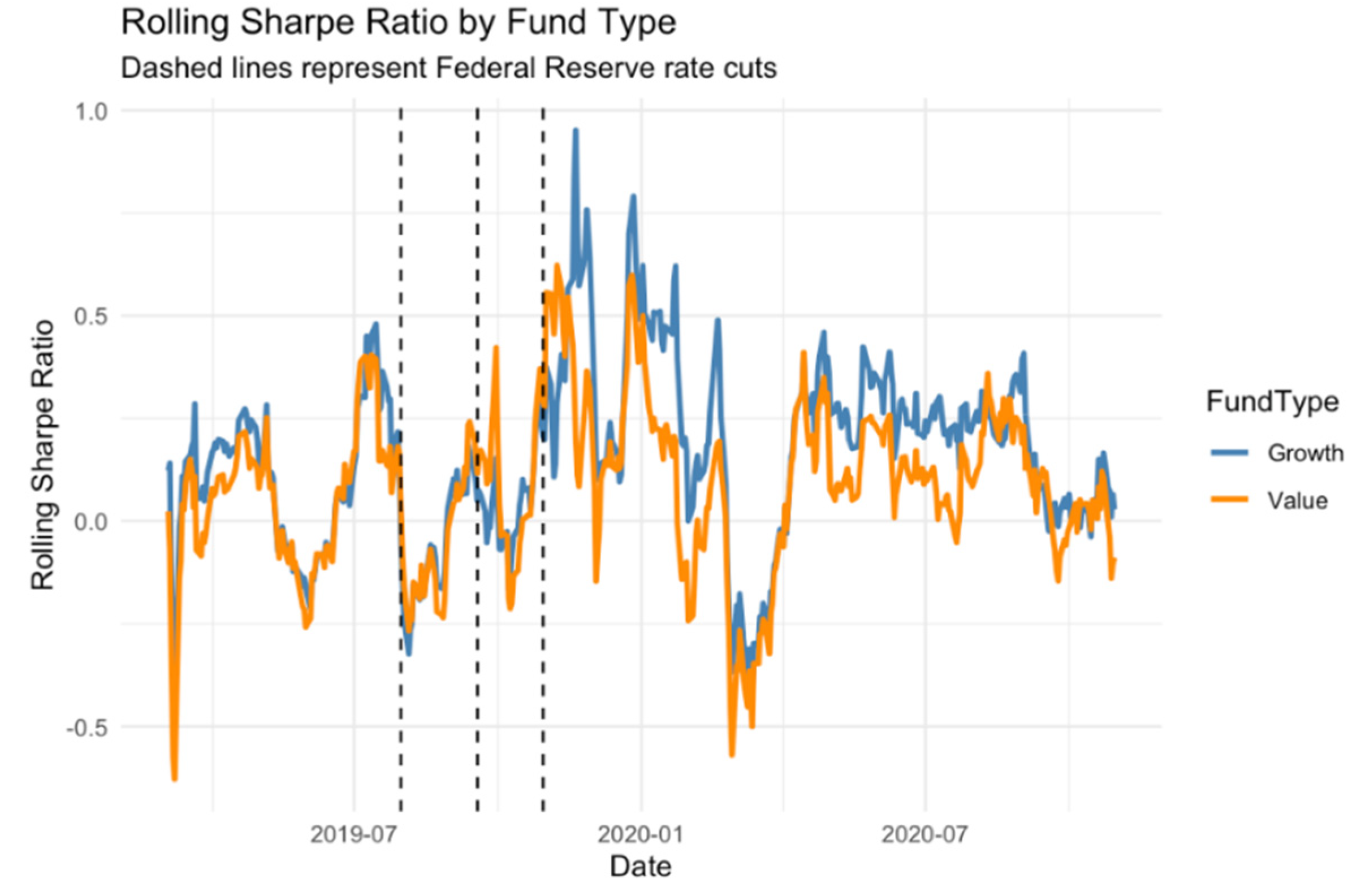
Figure 2.
Rolling Jensen’s Alpha by Fund Type.
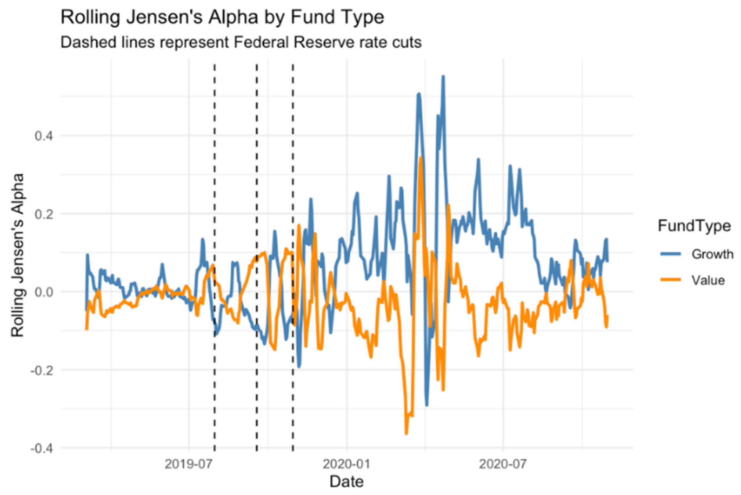
Table 1.
Fund Sample Selection Criteria.
| Fund Code | Fund Name | Style | Index/Active1 | AUM (B USD) 2 | Reason for Inclusion |
|---|---|---|---|---|---|
| VIGAX | Vanguard Growth Index Fund Admiral Shares | Growth | Index | Large | Pure growth style, low expense ratio |
| FDGRX | Fidelity Growth Company Fund | Growth | Active | Large | Aggressive growth focus, strong data trail |
| TRBCX | T. Rowe Price Blue Chip Growth Fund | Growth | Active | Large | Blue-chip, growth-oriented, liquid |
| VVIAX | Vanguard Value Index Fund Admiral Shares | Value | Index | Large | Pure value style, benchmark-like |
| DODGX | Dodge & Cox Stock Fund | Value | Active | Large | Classic value stock fund, long history |
| AWSHX | American Funds Washington Mutual Investors Fund | Value | Active | Large | Focus on dividend/value with stability |
1 indicates whether the fund follows a passive index-tracking strategy (Index) or is actively managed by fund managers (Active). 2 refers to the fund’s total Assets Under Management, expressed in billions of U.S. dollars, indicating the scale of the fund.
Table 2.
Key Variable Definitions.
| Variable | Definition |
|---|---|
| Fund Type | Make the four-fund type for all the observations which are growth, benchmark (SPX and VIX), and the policy (FFUNDS). |
| Close Price for Benchmarks Funds | End-of-day price of SPX or VIX, they only have the original close price without adjusted value, because they do not issue dividends. |
| Adjusted Net Asset Value | End-of-day fund NAV, adjusted for dividends and splits. Directly downloaded for each value and growth fund. |
| Net Asset Value Change (%) | Based on Modern Portfolio Theory (MPT),to compute daily return change for SPX and VIX, because they need daily returns to represent market movements. |
| Daily Policy Rate Change | . First-order difference of the Federal Funds effective rate in level terms. |
| Market Return | Using the SPX percent price change value as the market return. |
| Rolling Market Return (30-day) | We construct a 30-day rolling average of market returns for the SPX to identify short-term market trends consistent with the rolling Jensen Alpha calculation. |
| Rolling Volatility (30-day) | SD of the fund’s daily NAV change (%) over the past 30 trading days, measuring short-term variability. |
| Risk-free rate | Obtain TB3MS data from the FRED database and convert it to daily frequency using linear interpolation. To ensure consistency with daily returns, the annualized rates are further scaled by 1/252 to derive daily risk-free rates. |
| Beta | In the analysis, each fund’s daily returns are regressed against market returns on a one-time basis to derive a β-value that represents its average risk exposure over time. |
| Rolling beta | .is the daily return of the S&P 500 index. |
| Rolling a | 30-day CAPM intercept: intercept from the same rolling-window regression used to compute rolling β. |
| Rolling SR | computed within each 30-day moving window. is the average excess return within the 30-day window. is the sample SD of the daily NAV growth rate of the fund within the 30-day window, which measures its volatility. |
| AR | . The deviation of the fund’s return from its CAPM-predicted return on day t. Whereis the sensitivity of the fund to the market excess return estimated by the rolling regression of the past 30 days on day t. |
| CAR | . The daily AR of a fund i in each time interval is accumulated to obtain the CAR of the interval. |
| Event window dummies | Binary indicators equal to 1 if t falls within any specified window: • Pre-cut window (30 trading days before first cut) • Each short-term window (±30 days around each rate cut) • Six-month and one-year windows after October 30, 2019. |
| Fund style dummy | Equals 1 if fund is classified as Growth, 0 if Value. |
Table 3.
Sharpe-Ratio Model Specifications.
| Model ID | Dependent Variable | Specification | Purpose/Notes |
|---|---|---|---|
| S1 | Static SR | Baseline: compare overall risk-adjusted returns of Growth vs. Value | |
| S4 | 30-day Rolling SR | Dynamic: allow Sharpe to vary over time | |
| S4_w1–w5 | 30-day Rolling SR | Same as S4, estimated separately in each window w=1, … ,5 | Heterogeneity: test policy-window effects (Pre-Cut, Non-Event, Event1/2/3) |
| S5 | 30-day Rolling SR | Interaction: assess whether Growth/Value effect differs by period (Pre-Cut/Non-Event/Event) | |
| S6 | 30-day Rolling SR | Multivariate: control for volatility and market movement | |
| S8_interact | 30-day Rolling SR | Style×Market: examine how market swings modulate style premium |
Notes.
for Growth funds, 0 for Value. Windows w=1,...,5 correspond to Pre-Cut, Non-Event, Event1 (Jul 31), Event2 (Sep 18), Event3 (Oct 30). Period dummies indicate membership in each of the three event/non-event windows; S5 and S8 additionally cluster by fund.
Table 4.
Jensen’s Alpha Model Specifications.
| Model ID | Dependent Variable | Specification | Purpose / Notes |
|---|---|---|---|
| lm_model2 | Static a | Baseline CAPM a: compares Growth vs. Value | |
| lm_model4 | Rolling a | Time-varying a: simple rolling-window model by fund style | |
| lm_model3 | Rolling a | Adds market-return control | |
| lm_model3_interact | Rolling a | Style×Market interaction: tests heterogeneous a response to market swings | |
| lm_model6 | Rolling a | Multivariate: controls for both market-return and volatility | |
| lm_model6_interact | Rolling a | Style×Volatility interaction: examines whether risk fluctuations affect a differently by style | |
| lm_model12_interact | Rolling a | Event-window interactions captures a heterogeneity across Fed-cut windows (e.g., Window 2–3…) | |
| lm_model14 | Rolling a | Global style ×Period interaction: overall a differences across Pre-Cut / Non-Event / Event periods |
Notes.
for Growth funds, 0 for Value. is the market excess return (SPX log-return minus risk-free rate). indicates membership in event window w (e.g., Window 2 = ±30 days around Sep 18). are dummies for Pre-Cut, Non-Event, and Event periods.
Table 5.
Average CAR by Fund Style and Event Window.
| Event Windows | Growth CAR (Mean ± SD) | Value CAR (Mean ± SD) | N 1 |
|---|---|---|---|
| ±30 days (Event 1) | 0.84 ± 0.70 | –0.63 ± 0.80 | 132 |
| 6-month post-cut | 5.36 ± 4.94 | –2.40 ± 3.99 | 378 |
| 1-year post-cut | 14.64 ± 11.43 | –5.31 ± 6.81 | 762 |
1 N = number of fund-day observations in each window.
Table 6.
Growth vs. Value CAR Comparisons.
| Window | Growth CAR | Value CAR | t-statistic | p-value |
|---|---|---|---|---|
| ±30-day Event 1 | 0.84% | –0.63% | 15.92 | 0.000*** |
| 6-month post-cut | 5.36% | –2.40% | 23.73 | 0.000*** |
| 1-year post-cut | 14.64% | –5.31% | 41.39 | 0.000*** |
Note. Means and t-statistics are based on Welch’s t-test. The full results for all windows are presented in Appendix B Table A4. The p-value is reported to three decimal places (values < 0.001 shown as 0.000). Significance: * p < 0.10; ** p < 0.05; *** p < 0.01.
Table 7.
Interaction Regression of CAR on Fund Style and Period.
| Variable | Estimate | Robust SE | t-statistic | p-value |
|---|---|---|---|---|
| (Intercept) | 0.769 | 0.053 | 14.380 | 0.000*** |
| Value fund dummy | –1.113 | 0.071 | –15.683 | 0.000*** |
| Non-Event period | –0.016 | 0.093 | –0.168 | 0.000*** |
| Event period | 7.898 | 0.272 | 28.991 | 0.000*** |
| Value × Non-Event | –0.832 | 0.122 | –6.827 | 0.000*** |
| Value × Event | –10.820 | 0.312 | –34.718 | 0.000*** |
Note. Dependent variable: CAR over ± 30-day windows. Refer to Table 6 for the explanation of the p-value. Model fit: R2=0.344, Adjusted R2= 0.343, F(5,370) =388.4, p < 0.001. BP test: BP = 418.27 on 5 of df, p < 0.001.
Table 8.
Event-By-Event (Short-Term) CAR Regression Coefficients (Value vs. Growth).
| Event Date | Value vs. Growth Estimate | Robust SE | t-statistic | p-value |
|---|---|---|---|---|
| July 31, 2019 | –1.525 | 0.070 | –21.642 | 0.000*** |
| September 18, 2019 | 1.166 | 0.098 | 11.865 | 0.000*** |
| October 30, 2019 | –1.400 | 0.087 | –16.096 | 0.000*** |
Note. Refer to Table 6 for the explanation of the p-value.
Table 9.
Long-Term CAR by Fund Style.
| Horizon | Growth Mean CAR (%) | Value vs. Growth Estimate | Robust SE | t-statistic | p-value |
|---|---|---|---|---|---|
| 6-month post-cut | 4.943 | –7.146 | 0.219 | –32.593 | 0.000*** |
| 1-year post-cut | 10.938 | –15.040 | 0.355 | –42.383 | 0.000*** |
Notes. The estimate of the intercept term a (w) is called “Growth Mean CAR”, while the “Value vs. Growth Estimate” is β (w), which measures the differential between the CAR of value funds and growth funds. Refer to Table 6 for the explanation of the p-value.
Table 10.
CAR on Fund Style Controlling for Systematic Risk.
| Specification | Growth Dummy (γ) | SE (γ) | t-statistic (γ) | p-value (γ) | Beta (δ) | SE (δ) | t-statistic (δ) | p-value (δ) |
|---|---|---|---|---|---|---|---|---|
| Static β | 0.020 | 0.007 | 2.807 | 0.005** | –0.015 | 0.003 | –4.305 | 0.000*** |
| 30-day Rolling β |
0.193 | 0.008 | 24.604 | 0.000*** | –0.013 | 0.000 | –28.044 | 0.000*** |
| 60-day Rolling β |
0.140 | 0.008 | 17.743 | 0.000*** | –0.001 | 0.001 | –2.204 | 0. 028* |
Notes. Since the BP test significantly rejects equal variance in all models (p < 0.001). Refer to Table 6 for the explanation of the p-value. “Growth Dummy γ” denotes the average CAR difference (in percent) for growth relative to value; ‘Beta δ’ marginal effect after controlling for systematic risk.
Table 11.
Interaction of Fund Style and Beta on CAR.
| Specification | Intercept | GrowthDummy (γ) | SE (γ) | t (γ) | p (γ) | Beta (δ) | SE (δ) | t (δ) | p (δ) | Growth×Beta (θ) | SE (θ) | t (θ) | p (θ) |
|---|---|---|---|---|---|---|---|---|---|---|---|---|---|
| Static β | 0.981 | 0.011 | 0.002 | 4.52 | 0.000*** | –0.028 | 0.002 | –14.83 | 0.000*** | 0.0345 | 0.002 | 17.96 | 0.000*** |
| 30-day rolling β | 0.980 | 0.230 | 0.002 | 108.90 | 0.000*** | –0.0087 | 0.0002 | –57.27 | 0.000*** | –0.0084 | 0.0002 | –35.47 | 0.000*** |
Notes. Dependent variable: CAR over ± 30-day windows. Refer to Table 4 for the explanation of the p-value.
Table 12.
Static and Full-Sample Rolling Sharpe-Ratio Regressions.
| Model | Description | Growth Dummy γ | Robust SE | t-statistic | p-value |
|---|---|---|---|---|---|
| S1 | Static SR ~ FundType | –0.048556 | (0.000124) | –390.220 | 0.000*** |
| S4 | Rolling SR ~ FundType | –0.088672 | (0.003556) | –24.933 | 0.000*** |
Note. Refer to Table 8 for the explanation.
Table 13.
Rolling Sharpe-Ratio by Event Window.
| Window | Growth Dummy γ | Robust SE | t-statistic | p-value |
|---|---|---|---|---|
| Pre-Cut (30 days) | –0.051144 | (0.005809) | –8.805 | 0.000*** |
| Event 1 (±30 days around Jul 31) | –0.050106 | (0.007578) | –6.612 | 0.000*** |
| Event 2 (±30 days around Sep 18) | –0.023576 | (0.005058) | –4.662 | 0.000*** |
| Event 3 (±30 days around Oct 30) | –0.071145 | (0.004760) | –14.947 | 0.000*** |
| 6-month post-cut | –0.101660 | (0.004181) | –24.313 | 0.000*** |
| 1-year post-cut | –0.101410 | (0.004054) | –25.013 | 0.000*** |
Note. Refer to Table 8 for the explanation.
Table 14.
Interaction With Period Indicators (Model S5).
| Term | Estimate | Robust SE | t-statistic | p-value |
|---|---|---|---|---|
| Growth Dummy | –0.051144 | (0.008212) | –6.228 | 0.000*** |
| Non-Event period | –0.231543 | (0.011539) | –20.067 | 0.000*** |
| Event period | –0.001333 | (0.006474) | –0.206 | 0.836 |
| Growth × Non-Event | –0.002064 | (0.016372) | –0.126 | 0.900 |
| Growth × Event | –0.039808 | (0.009020) | –4.413 | 0.000*** |
Note. Refer to Table 8 for the explanation.
Table 15.
Multivariate Controls (Model S6).
| Term | Estimate | Robust SE | t-statistic | p-value |
|---|---|---|---|---|
| Growth Dummy | –0.086982 | (0.002911) | –29.883 | 0.000*** |
| 30-day Rolling Volatility | 0.016520 | (0.001343) | 12.303 | 0.000*** |
| 30-day Market Excess Return | 0.648150 | (0.007392) | 87.682 | 0.000*** |
Note. Refer to Table 8 for the explanation.
Table 16.
Style × Market-Return Interaction (Model S8_interact).
| Term | Estimate | Robust SE | t-statistic | p-value |
|---|---|---|---|---|
| Growth Dummy | –0.083092 | (0.002926) | –28.397 | 0.000*** |
| Rolling Market Excess Return | 0.657687 | (0.007461) | 88.153 | 0.000*** |
| Growth × Rolling Market Excess Return | –0.122932 | (0.009976) | –12.322 | 0.000*** |
Note. Refer to Table 8 for the explanation.
Table 17.
Style Effect on Jensen’s Alpha.
| Model ID | GrowthDummy γ | Robust SE | t-statistic | p-value | Controls |
|---|---|---|---|---|---|
| lm_model2 | –0.103952 | (0.000291) | –358.09 | 0.000*** | None (Static a) |
| lm_model4 | –0.092289 | (0.001891) | –48.80 | 0.000*** | None (Rolling a) |
| lm_model3 | –0.092289 | (0.001889) | –48.85 | 0.000*** | + Rolling_Market_Return |
| lm_model6 | –0.090839 | (0.001884) | –48.21 | 0.000*** | + Rolling_Market_Return+ Rolling_Volatility |
Note. Refer to Table 8 for the explanation.
Table 18.
Key Interaction Terms in Jensen’s Alpha Models.
| Model | Interaction Term | Estimate | Robust SE | t-statistic | p-value | Controls |
|---|---|---|---|---|---|---|
| lm_model3_interact | GrowthDummy × Rolling_Market_Return | 0.089273 | (0.012871) | 6.936 | 0.000*** | Rolling_Market_Return |
| lm_model6_interact | GrowthDummy × Rolling_Volatility | –0.034150 | (0.002440) | –13.994 | 0.000*** | Rolling_Market_ReturnRolling_Volatility |
| lm_model12_interact | GrowthDummy × D_Window_2 (Sep 18) | –0.137113 | (0.004985) | –27.504 | 0.000*** | Event Windows |
| GrowthDummy × D_Window_3 (Oct 30) | 0.132835 | (0.004199) | 31.634 | 0.000*** | ||
| GrowthDummy × D_Long_6M | –0.014585 | (0.007312) | –1.995 | 0.046* | ||
| GrowthDummy × D_Long_1Y | –0.140386 | (0.006767) | –20.747 | 0.000*** | ||
| lm_model14 | GrowthDummy × PeriodEvent (Event) | –0.081244 | (0.004554) | –17.840 | 0.000*** | Period Dummies (Pre-Cut/Non-Event/Event) |
Notes. Refer to Table 8 for the explanation. Interaction specifications are also clustered by fund. “Controls” lists additional regressors included in each model beyond GrowthDummy. D_Window_2 = ±30 days around Sep 18; D_Window_3 = ±30 days around Oct 30; D_Long_6M/1Y are 6-month/1-year post-cut dummies.
Disclaimer/Publisher’s Note: The statements, opinions and data contained in all publications are solely those of the individual author(s) and contributor(s) and not of MDPI and/or the editor(s). MDPI and/or the editor(s) disclaim responsibility for any injury to people or property resulting from any ideas, methods, instructions or products referred to in the content. |
© 2025 by the authors. Licensee MDPI, Basel, Switzerland. This article is an open access article distributed under the terms and conditions of the Creative Commons Attribution (CC BY) license (http://creativecommons.org/licenses/by/4.0/).
Copyright: This open access article is published under a Creative Commons CC BY 4.0 license, which permit the free download, distribution, and reuse, provided that the author and preprint are cited in any reuse.


