Submitted:
27 November 2025
Posted:
28 November 2025
You are already at the latest version
Abstract
We formulate Temporal Dynamics (TD), a clock-first description in which a universal space–growth speed S(t) sets the causal baseline and a dimensionless slow–time field ΔT(x, t) encodes local rate loss. In the quasistatic, weak field we use a single scalar to control kinematics and optics: g = −(S2/2)∇ΔT and n(x) = 1/p 1 − ΔT(x). With the Normalization Axiom S ≡ c and the identification N2 = 1 − ΔT, TD reproduces GR’s tested content (Newtonian limit, gravitational redshift, Shapiro delay, light deflection, and standard GW degrees of freedom) without introducing a new propagating mode. Horizons occur at ΔT→1, fixing the global mass–size calibration DBH = 4GM/c2. The source law uses the GR weak-field “active density” ρ + (px + py + pz)/c2, cleanly separating EM propagation (via n) from sourcing (via stresses). Allowing a tiny homogeneous clock drift ε(t) = ˙S/c yields an effective Λ(t) = 3ε(t)2/c2, a one-parameter extension of ΛCDM with distances E2(z) modified by (1 + z)2p. We outline a falsifiable program: map ΔT(x) with clock networks and atom interferometers, test the optical dictionary on engineered links and lensing, and fit the cosmological parameter p with SNIa, BAO, and H(z), cross-checking growth and the turnaround scale r∗ = (GM/ε2)1/3.
Keywords:
temporal Dynamics
; lapse N
; gravitational redshift
; Shapiro delay
; gravitational lensing
; optical clocks
; atom interferometry
; dark energy
1. Introduction
General Relativity (GR) describes gravity extraordinarily well in terms of spacetime geometry and has passed a wide range of precision tests[1,2,3]. In this paper we present a native formulation of Temporal Dynamics (TD) in which a universal space–growth clock produces adjacency. The clock has baseline speed (m s−1), and mass–energy creates a dimensionless slow–time field that locally taxes the clock. Kinematics and optics then follow from this single field: bodies fall down gradients of , and light propagates as if vacuum had an index , reproducing the standard weak-field lensing picture[4]. (For TD background and motivation see Ref. [5].)
- Thesis (cause → representation).
When the baseline is frozen to a constant and the ADM lapse is identified by
TD reproduces GR’s tested content (Newtonian limit, gravitational redshift, Shapiro delay, lensing, and gravitational waves) without introducing new degrees of freedom[1,6,7,8,9,10,11,12,13]. In this sense, GR is the representation of a clocked universe under a frozen baseline; TD supplies the cause. Allowing a tiny uniform drift yields an effective dark–energy term
which reduces to GR+ when is constant and vanishes when ; observationally, a constant term is consistent with supernovae and BAO evidence for late-time acceleration[14,15,16].
- Operational content.
The field is defined by clock comparisons: for static observers with N from (1). Classical and modern redshift tests (Mössbauer, optical clocks, satellite clocks) implement precisely this comparison[17,18,19,20,21]. With normal matter and appropriate boundary conditions (asymptotic flatness), outside horizons. The endpoint marks a black boundary (lapse ); it is distinct from the “pre-clock” state , in which spacetime is not yet operationally defined.
- Minimal laws used throughout.
In the quasistatic, weak-field regime TD uses:
The source combination in (5) (pressures gravitate) is the standard weak-field GR result[22]. With the weak-field identification and the Normalization Axiom , Eq. (4) gives exactly Newton’s law. The horizon calibration sets the black-boundary diameter
consistent with the Schwarzschild limit[2,3] and explicitly used in the TD ↔GR bridge[13].
- What this paper does (and does not) claim.
- Cause: We posit a physical clock that produces adjacency; is a measurable field that encodes local slow–time.
- TD-specific handle: A tiny uniform drift (clock drift) appears as in (2) and leads to the turnaround scale separating bound from unbound flow.
- Scope and structure.
Section 2 states the axioms and normalizations (including the necessity of in our epoch for empirical calibration). Section 3 gives an operational definition of and its domain of validity. Section 4 derives Newton’s law and collects the TD→observable dictionary. Section 5 treats optical tests via the index . Section 6 discusses horizons and the mass–size law. Section 7 incorporates pressures in sourcing and clarifies why mass typically produces steeper local slow–time gradients than radiation. Section 8 points to the GR bridge note. Section 9 places classical electromagnetism on a TD background (propagation vs. sourcing). Section 10 lists quantum-ready observables (clocks and interferometers). Section 11 treats cosmology (clock drift, genesis picture, and key scales). Section 12 outlines laboratory and astronomical tests; Section 13 addresses common objections; Section 14 states limitations; Section 15 concludes. A compact notation reference is given in Appendix H, Table H.
2. Axioms and Normalization
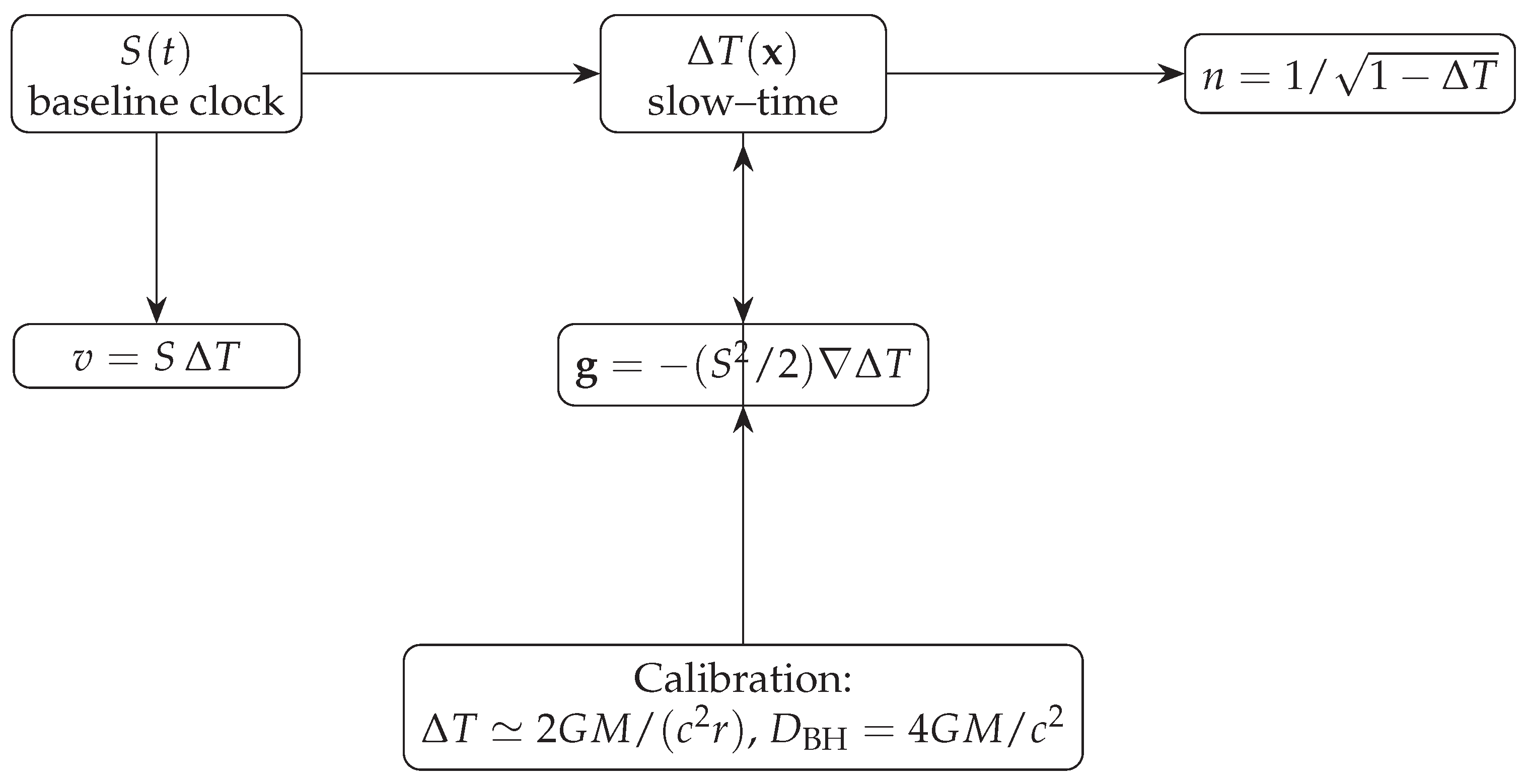
This section states the primitive quantities and the minimal laws of Temporal Dynamics (TD). We keep the presentation quasistatic and weak field unless stated otherwise; dynamical refinements can be added later without changing the calibration logic. A compact summary of axioms and references is given in Table 1. A schematic of the relations between primitives, kinematics, optics, and calibration is shown in Figure 1; the horizon calibration is illustrated in Figure 2.
2.1. Primitives and Units
- Axiom A (Clock / space–growth). There exists a baseline space–growth speed (m s−1) representing the universal production of adjacency per unit cosmic time. In the bridge regime it will be frozen to a constant (§2.6).
2.2. Kinematics and Gravity (Quasistatic)
- Axiom C (Kinematics). The peculiar speed of a test body relative to the baseline is
- Axiom D (Gradient law for gravity). In a quasistatic field the gravitational acceleration is
2.3. Sourcing by Stress–Energy (Active Density)
-
Axiom E (Poisson law, weak/static). Outside sources and for with slow time variation,
2.4. Optics: Index of Time
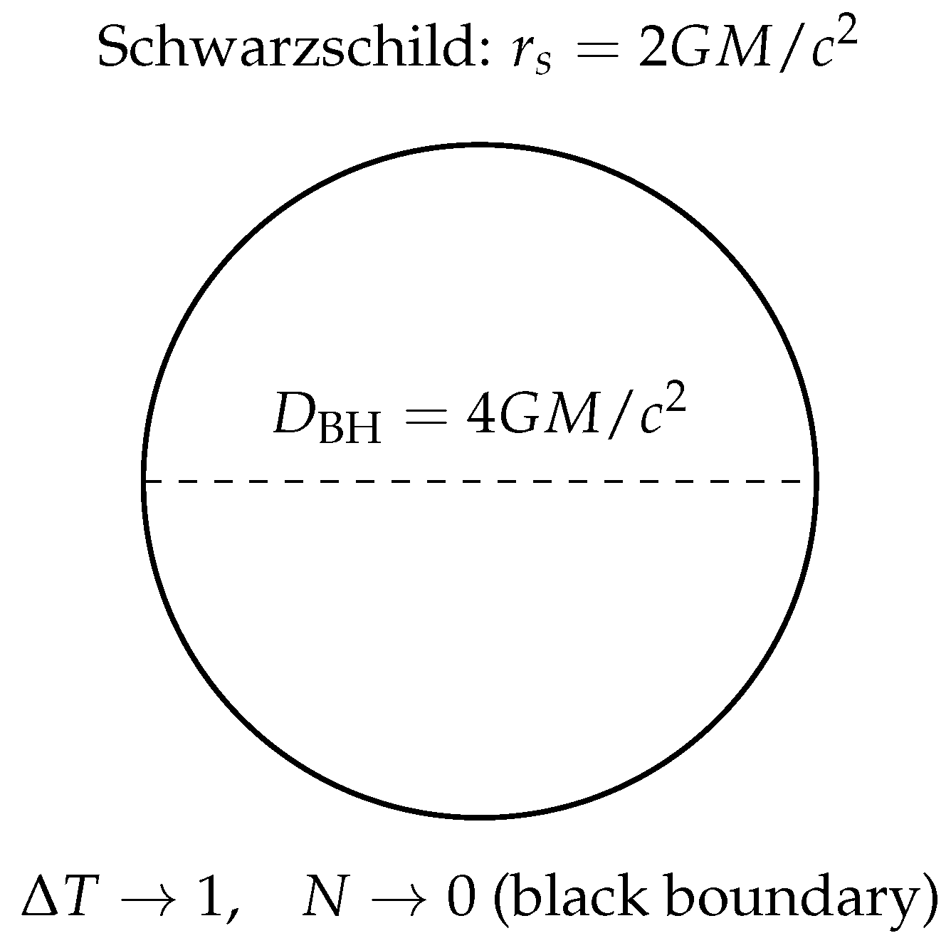
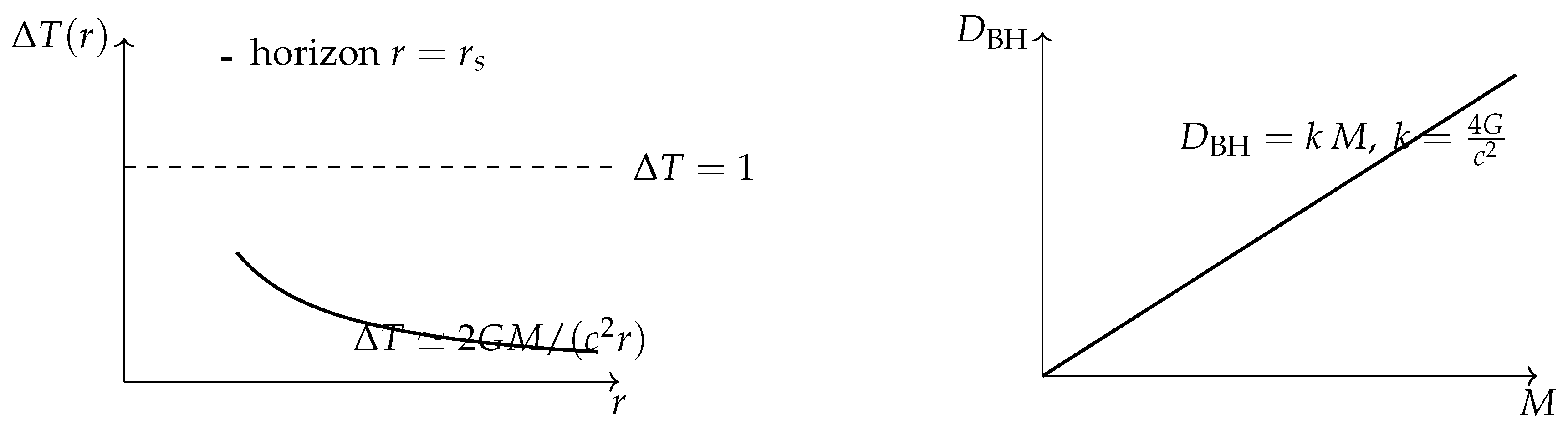
2.5. Horizon Calibration
-
Axiom G (Black boundary). The surface defines a black boundary (static lapse ). Matching to the Schwarzschild scale fixes the global calibration constant
2.6. Normalization and Necessity of
The empirical calibrations used throughout are:
Inserting the first of (14) into the gradient law (10) fixes the overall scale:
- Normalization Lemma. To recover Newton’s law exactly from Eq. (15), the baseline must satisfy . See Appendix B and the bridge note[13].
- Comment. Choosing a constant while keeping (14) would mis-scale gravity by . One could re-define the calibrations with , but that is merely a change of symbols. In the realized epoch we therefore impose the Normalization Axiom:
2.7. Domain and Boundary Conditions (Summary)
We adopt asymptotic flatness so that and at spatial infinity. For normal (positive) energy densities and static exteriors, the elliptic maximum principle implies
The endpoint marks a horizon (black boundary). The pre-clock boundary is distinct: before the clock turns on, neither t, , nor are operationally defined[2,3]. A full operational construction of from clock networks is provided next (Section 3).

Table 1.
TD axioms and key formulas. Each axiom is referenced in-text; standard GR/optics references are cited where appropriate.
Table 1.
TD axioms and key formulas. Each axiom is referenced in-text; standard GR/optics references are cited where appropriate.
| Axiom | Content | Key relation / cite |
|---|---|---|
| A | Baseline clock | Normalization Axiom |
| B | Slow–time & lapse | (8); ADM[6,7] |
| C | Kinematics | (9) |
| D | Gravity (gradient law) | (10) |
| E | Source law (weak/static) | Eq. (11); [1,22] |
| F | Optics (index of time) | (12); [4,8] |
| G | Horizon calibration | (13); [2,3] |
Figure 1.
Schematic of TD primitives and observables. Baseline and slow–time field feed kinematics and optics ; calibration enters through and . This diagram summarizes Eqs. (9)–(12) and (14).
3. Operational Definition of
This section defines purely from clock comparisons and signal transfer, tying the field to observables and keeping it coordinate–independent. We assume quasistatic conditions (negligible frame dragging at the measurement scale) and work in the exterior of horizons.
3.1. Clocks, Rates, and the Lapse
For static observers, proper time satisfies with (Eq. (8); N is the ADM lapse[6,7]). Consider two co–stationary clocks at events A and B connected by a phase–coherent link (optical fiber, microwave, or free–space two–way). Let and be the locally measured transition frequencies of identical standards. In the quasistatic limit,
Equation (18) defines differences of from clock data. When ,
This relation is the basis of gravitational redshift tests from Mössbauer/Pound–Rebka to modern optical clocks and satellites[17,18,19,20,21].
3.2. Local Gradients from Frequency Maps
A dense network of clocks provides a scalar field whose spatial gradient yields directly. Taking the differential of Eq. (18) and linearizing,
Combined with the TD gradient law (Eq. (10)) this gives a fully operational expression for the gravitational acceleration:
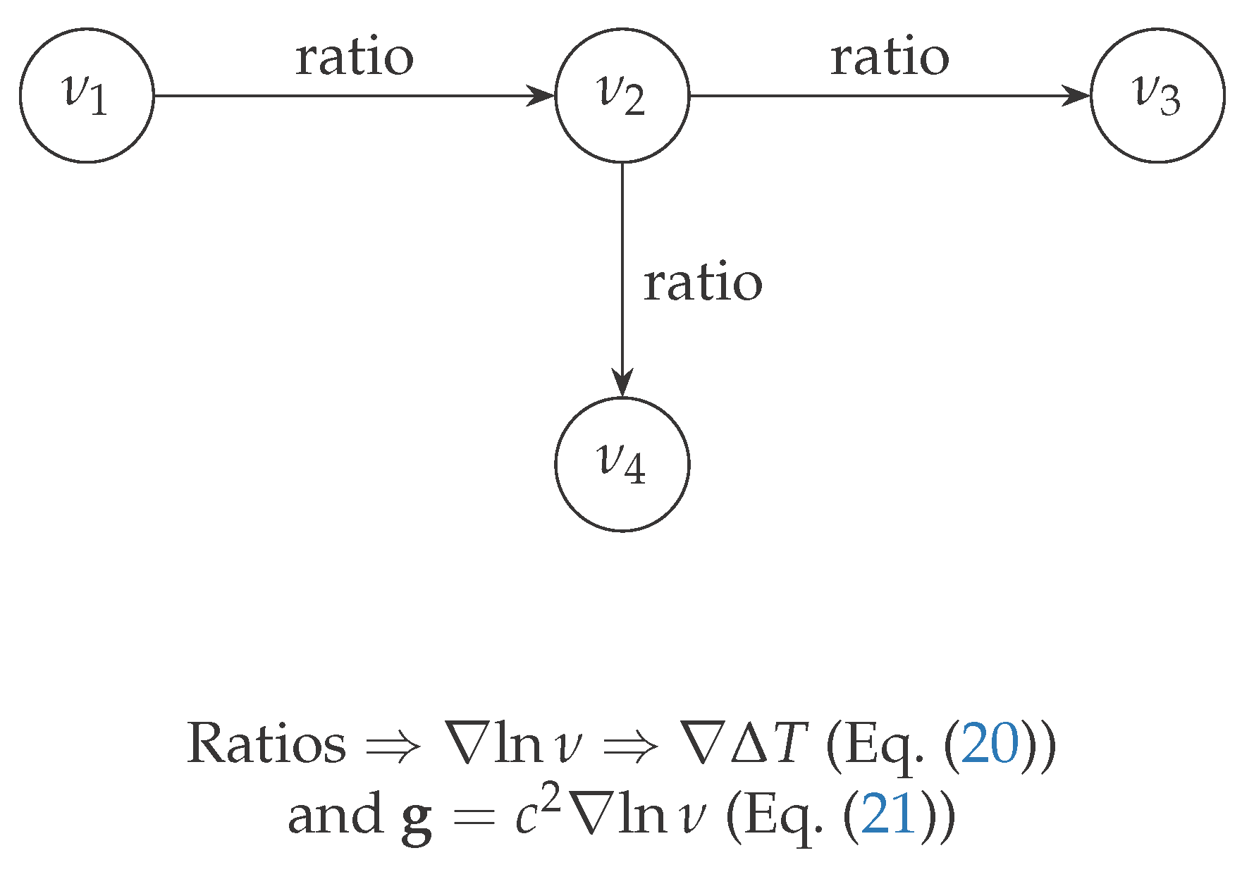
In words: the spatial derivative of the log clock frequency equals the local gravitational field divided by . This is coordinate–free and depends only on what co–located observers read from their instruments. A schematic of the mapping pipeline is shown in Figure 3.
3.3. Reconstructing (Dirichlet/Neumann)
Absolute values follow by fixing a boundary condition. With asymptotic flatness at large radius, one can integrate Eq. (20) along any path from infinity to ,
On finite laboratory domains, either
- Dirichlet: set on a reference surface (e.g., from an exterior model) and integrate inward, or
- Neumann: measure (via vertical clock gradients) on the boundary and solve the Poisson problemfor the region of interest (cf. Eq. (11)).
3.4. Practical Measurement Protocol
- Clock grid. Deploy identical (or cross–calibrated) clocks at positions ; record with traceable time transfer (two–way fiber/microwave or common–view)[24].
- Frequency ratios. Compute for neighboring pairs to suppress common–mode noise.
- Gradient estimation. Fit over local baselines (finite–difference or regression); propagate uncertainties from the Allan deviations of the clocks and links.
3.5. Domain, Validity, and Limits
- Range. With normal matter and exterior boundary conditions, (Eq. (17)). The endpoint corresponds to a black boundary where and static observers cease to exist.
- Independence of coordinates. The construction uses only ratios of locally measured frequencies and spatial differences taken along a physical baseline; coordinates are bookkeeping for plotting and PDE solvers.
3.6. Horizon and Pre–Clock Distinctions
Approaching a horizon, and for a static link crossing outward to inward (Eq. (18)); . By contrast, in the pre–clock state no operational time or space exists, and is undefined. The two limits must not be conflated.
4. Kinematics and Gravity from
This section shows how TD turns the slow–time field into motion and standard observables. We work in the quasistatic, weak–field regime and use the normalization from Eq. (16).
4.1. Newton’s Law from the Gradient of
Outside an isolated mass M, the weak–field identification is
Taking the spatial gradient and using the TD gradient law (Eq. (10)) yields
with directed inward (toward decreasing r). Thus TD reproduces Newton’s inverse–square law exactly in the weak field, consistent with standard GR[1,2,3].
- Numerical check (Earth).
4.2. TD → Observables: the Minimal Dictionary
In TD the same scalar governs mechanical and optical effects. To leading order in : The minimal dictionary used throughout is summarized in Table 3.
These expressions reproduce the standard weak–field GR results[1] when is used for an isolated mass.
4.3. Quick Numerical Checks (Optics and Timing)
- (a)
-
Gravitational redshift over on Earth.
- (b)
-
Shapiro delay for a ray grazing the Sun (one–way).
- (c)
-
Light deflection by the Sun at the limb.With , the small–angle integral yieldsthe classic Eddington value[10].
4.4. Ray Picture (Index of Time): A Visual
4.5. Remarks
- Beyond the weak/quasistatic regime, the same observables can be phrased in terms of the full with shift and spatial metric where needed; results coincide with GR in the bridge limit[1].
5. Optical Tests via the Index
In TD a static, weak field acts like an isotropic medium with effective refractive index
cf. Eq. (12). Light rays extremize the coordinate travel time
which is Fermat’s principle in the TD/optical-metric picture (equivalent to the weak-field GR optical metric[1,4]). All standard optical tests follow from (27)–(28).
5.1. Gravitational Redshift
5.2. Shapiro Time Delay
5.3. Light Deflection (Small Angle)
Let be the unit tangent to the ray. The Euler–Lagrange equation for (28) yields the isotropic ray equation
Projecting perpendicular to the unperturbed direction and integrating along the path gives the net deflection
to first order in . For a point mass,
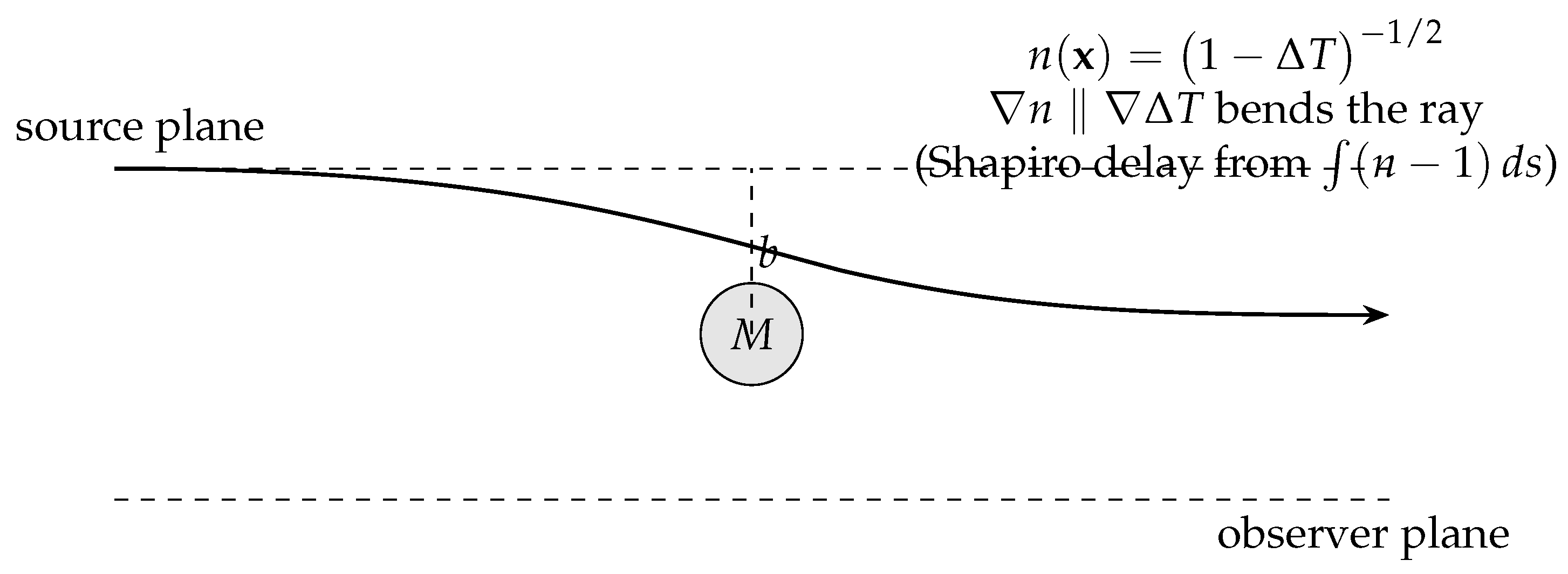
the classic solar-limb value when [1,4,10]. The lensing geometry and small-angle deflection are illustrated in Figure 5.
5.4. Remarks on Validity and Coordinates
- The optical construction is coordinate-clean: is the physical arclength on the slice and is a scalar built from .
- TD keeps cause/effect explicit: sources → via the Poisson law; →n sets all optical propagation.
Figure 5.
Lensing geometry in the index-of-time medium. Gradients of (set by ) deflect light by and produce the Shapiro delay; both recover the standard GR values in the weak field.
Figure 5.
Lensing geometry in the index-of-time medium. Gradients of (set by ) deflect light by and produce the Shapiro delay; both recover the standard GR values in the weak field.
6. Horizons and the Mass–Size Law
In TD, horizons appear when the local slow–time share saturates the causal budget. This section defines the black boundary via , connects it to observable signatures, and states the linear mass–size calibration used as a global anchor for the framework.
6.1. Black Boundary: (lapse )
For static observers with (Eq. (8)). The surface
is a black boundary: a static worldline cannot be extended across it and the redshift from just outside to far away diverges[2,3]. In the TD optical picture the effective index (Eq. (12)) diverges there, so the coordinate travel time blows up (Shapiro delay ) for paths that attempt to linger on the boundary. The profiles and the linear mass–size law are shown in Figure 6.
6.2. Spherically Symmetric Exterior and Monotonicity
For a compact, nonrotating, uncharged source, the weak–field identification
increases monotonically inward. Its radial derivative, (with r increasing outward), guarantees that grows toward the center. With at infinity and positive (Eq. (11)), one has in the exterior, approaching 1 only at a horizon[1,22].
6.3. Mass–Size Calibration (Nonrotating Case)
Matching the TD boundary to the Schwarzschild event horizon fixes the linear mass–size law used throughout TD:
Equation (36) is identical to Eq. (13) and serves as a single global calibration linking the slow–time normalization to the observed mass scale of black boundaries[2,3]. Observationally, horizon–scale imaging (e.g. M87*) is consistent with the GR horizon scale used here[25].
- Remarks.
6.4. Operational Signatures of Approaching a Black Boundary
Let A be far away () and B approach the boundary along a static worldline. Then
Equations (37)–(39) summarize the TD optics/clock behavior: infinite redshift to infinity, divergent coordinate delay, and an unbounded index at the surface .
6.5. Pre–Clock Boundary vs. Black Boundary
It is important not to conflate:
- Pre–clock: (no baseline production of adjacency) before the universe begins; neither t, , nor are operationally defined.
- Black boundary: with already in place; static clocks stall locally (), but the baseline runs elsewhere.
Only the latter appears in astrophysical settings.
6.6. Cosmological (de Sitter–Type) Horizon from Clock Drift
A uniform baseline drift (with small, nearly constant ) induces an effective cosmological term (Eq. (2)). The associated cosmological horizon has radius
distinct in origin from the local black boundary of Eq. (34). The former is a global feature of an expanding baseline; the latter is a local saturation near compact mass. The turnaround/balance scale introduced later (cosmology section) marks where the DE push equals the local slow–time gradient pull.
7. Stress–Energy, Pressures, and Back–Reaction
Mass–energy does two things in TD: it propagates through a given slow–time landscape (via the index ) and it sources the slow–time field that shapes that landscape. This section formalizes the sourcing side, including the role of pressures, and gives practical magnitudes from laboratory to astrophysical settings.
7.1. Active Density and the TD Source Law
In the weak, static regime TD uses the Poisson–type source law (Eq. (11))
where is energy density and are principal pressures. For an isotropic fluid (),
Special cases used repeatedly:
Equations (41)–(44) mirror the standard weak–field GR result that pressures gravitate in addition to energy density[1,22]. The active-density cases used repeatedly are summarized in Table 4.
7.2. Electromagnetic Fields as Sources
Electromagnetic fields contribute through their energy and stresses. With
the Maxwell stress tensor implies (tracefree EM tensor), hence even for anisotropic static fields[26]. Free, isotropic radiation is the familiar case with and the same factor of 2 via Eq. (44).
- Propagation vs. sourcing (separation of roles).
Propagation: light follows Fermat in the effective index (Eq. (12)); this is how EM feels a given (Sec. 5).
Table 4.
Active density for common sources (weak, static TD; cf. Eq. (42)). EM fields are tracefree so even when anisotropic. A cosmological constant (vacuum energy) is not part of the local static Poisson problem but is shown for intuition; it gives negative active density and appears in TD as clock drift (Sec. 11).
| Source | EoS / stresses | |
|---|---|---|
| Cold matter (dust) | ||
| Radiation / photon gas | ||
| Stiff fluid | ||
| Electromagnetic field (static) | tracefree T: | |
| Vacuum energy () |
7.3. Why Rest Mass Usually “Slows Time More” in Practice
Per unit energy density, free radiation sources as strongly as (indeed twice as much as) cold matter [Eq. (44) vs. Eq. (43)]. In real systems, however, rest mass typically produces steeper local gradients because:
- Localization/compactness: rest mass can be packed and held in small R, creating large . Free radiation streams at c unless confined.
- Persistence: rest mass sources are steady in their rest frame; transient radiation passes quickly, making its contribution fleeting at a given point.
- Confinement bookkeeping: radiation in a box has pressure balanced by negative stresses of the walls; the net active mass of the isolated system is . Boxes cannot be made arbitrarily compact without collapse, limiting achievable compactness relative to dense matter.
7.4. Practical Magnitudes
- Laboratory field (1 T magnet).
Using ,
The resulting and its gradients are utterly negligible on laboratory scales (far below current clock sensitivities), though the concept is important.
- High–intensity laser focus (illustrative).
With intensity I, the energy density is . Even for ,
still tiny gravitationally over micron–millimeter focal volumes.
- Magnetar–scale field.
For ,
Over a region of size , the EM contribution alone would yield a surface–scale slow–time fraction of order
small compared to the star’s baryonic gravity but no longer negligible as a correction in principle.
7.5. Back–Reaction Remains Linear at Small
7.6. Equivalence Principle and Local Lorentz Invariance
TD respects local Lorentz invariance in the bridge regime () and, in the weak field, couples test bodies universally through via Eq. (10). The “active density” that sources is the same combination that appears in weak–field GR[1,22]. No composition–dependent forces arise beyond standard tidal effects contained in .
7.7. Summary (Sourcing vs. Propagation)
- Sourcing: mass–energy (including pressure) creates slow time via Eq. (41); the size of near a source is controlled primarily by compactness and persistence.
- Propagation: light and fields traverse a given landscape with effective index , producing redshift, delay, and bending as in Sec. 5.
- Practicality: EM back–reaction is negligible in labs but conceptually essential; in extreme astrophysics it can be a small, principled correction to the dominant baryonic/degenerate matter sourcing.
8. Relation to GR (Bridge Pointer)
This section states—without re-deriving—how TD reproduces the tested content of GR when the baseline is frozen and variables are repackaged. Full algebra and degree-of-freedom (DoF) counting are provided in a separate bridge note[13].
8.1. Dictionary (Frozen Baseline)
Set the baseline to its calibrated value (Normalization Axiom, Eq. (16)):
and identify the ADM lapse with the slow–time field via
The spatial metric and the shift are unchanged (standard split[6,7]). With Eq. (47), the TD optical and kinematic relations (Secs. 4–6) coincide with the standard GR weak–field formulas (Newtonian limit, gravitational redshift, Shapiro delay, light deflection)[1,4,8].
8.2. Action–Level Sketch and Constraints
In form, the Einstein–Hilbert action reads[6,7]
where , is the Ricci scalar of , and is the extrinsic curvature. Substituting and varying gives, schematically,
so the lapse variation (Hamiltonian constraint) is reproduced up to the nonzero multiplicative factor . The momentum constraint (variation of ) and the evolution equations (variation of ) are unchanged by the field redefinition. Thus the primary/secondary constraints and their algebra remain those of GR[6,7]; is a reparameterization of the lapse, not a new propagating field. A compact notation reference is given in Appendix H, Table H.
- Constraints (for reference).
The Hamiltonian and momentum constraints keep their GR form,
with matter energy density and momentum density measured by the N–normal observers (notation fixed here; derivation not repeated).
8.3. Degrees of Freedom and Gauge
Because N is nondynamical in GR (a Lagrange multiplier), the redefinition does not introduce a new radiative DoF. Linearizing around Minkowski (, , , ) yields the standard two tensor polarizations propagating at c; any lapse perturbation is gauge (non-propagating)[1,3]. Hence TD in the bridge regime has the same local Lorentz invariance and GW content as GR, consistent with observations[11,12].
8.4. PPN and Tested Weak–Field Phenomenology
With and Eq. (47), the Parametrized Post-Newtonian (PPN) parameters in the weak field are
and the classic tests are reproduced:
- Newtonian limit from with ;
- gravitational redshift ;
- Shapiro delay ;
- light deflection ,
8.5. Rotating Solutions (Kerr) and the Lapse
For stationary, axisymmetric spacetimes the metric in form involves . The bridge identifies
where is the lapse of the chosen foliation (e.g., Boyer–Lindquist or horizon–penetrating slices). Since TD leaves and untouched, all Kerr observables (ISCO, lensing, redshift, frame dragging) are inherited from the GR solution in the same slice[2,3]. The surface matches the behavior at the horizon.
8.6. Gravitational Waves
8.7. Scope and Limits of the Bridge
The mapping assumes (i) (frozen baseline), and (ii) regions where (outside horizons in the chosen slicing). Inside horizons a different foliation is required; TD treats that by construction via the boundary (Sec. 6). Cosmological applications that allow a tiny uniform drift fall outside the strict bridge (since ), but their homogeneous effect can be summarized by
and treated observationally as GR+ (Sec. 11).
Pointer to companion note
A separate bridge note[13] provides: (i) the explicit substitution of Eq. (47) into Eq. (48); (ii) the chain–rule variation Eq. (49) and the unchanged constraint algebra; (iii) a linear PPN calculation confirming ; (iv) a Kerr checklist in Boyer–Lindquist and Kerr–Schild slices; and (v) the GW linearization showing only two tensor modes at speed c.
9. Electromagnetism on a TD Background
Electromagnetism (EM) interacts with TD in two clean ways: (i) propagation—light and EM waves travel in a vacuum that behaves like a medium with index set by the slow–time field ; (ii) sourcing—EM energy and stresses contribute (weakly) to the field equation that determines . This section writes both pieces in a compact, operational form.
9.1. Maxwell on a Static TD Slice: Effective Medium
On a static slice with lapse N and spatial metric ,
vacuum electrodynamics is equivalent to Maxwell in an isotropic medium with[1,4,27,28]
and relative parameters (so the vacuum impedance remains ). Writing , , the macroscopic Maxwell system becomes
When varies slowly in time (quasistatic TD) the modification is the spatial dependence in Eqs. (58)–(59); the local light speed measured by comoving observers remains c, while the coordinate phase/group speeds are .
9.2. Wave, Ray, and Redshift Relations
In the geometric–optics limit (slowly varying n), the eikonal S obeys , and the travel time functional is Fermat’s
so rays satisfy and bend toward larger n (larger ), reproducing Eqs. (30)–(33). For scalar envelopes (ignoring polarization) one may use the Helmholtz form
with amplitude transport corrections when is not negligible.
Clock comparisons are set by the lapse (not by n): for static observers
as in Eq. (29). Thus TD cleanly separates propagation (via n) from rate (via N).
9.3. Sourcing of by EM
EM fields gravitate through their energy density and stresses. With
the weak, static TD source law (Eq. (41)) gives
so free, isotropic radiation () contributes , and more generally trace–free EM stresses imply [26]. In laboratories this back–reaction is negligible; in extreme astrophysics (magnetars, pair fireballs) it can be a principled correction.
9.4. Two Compact Observables
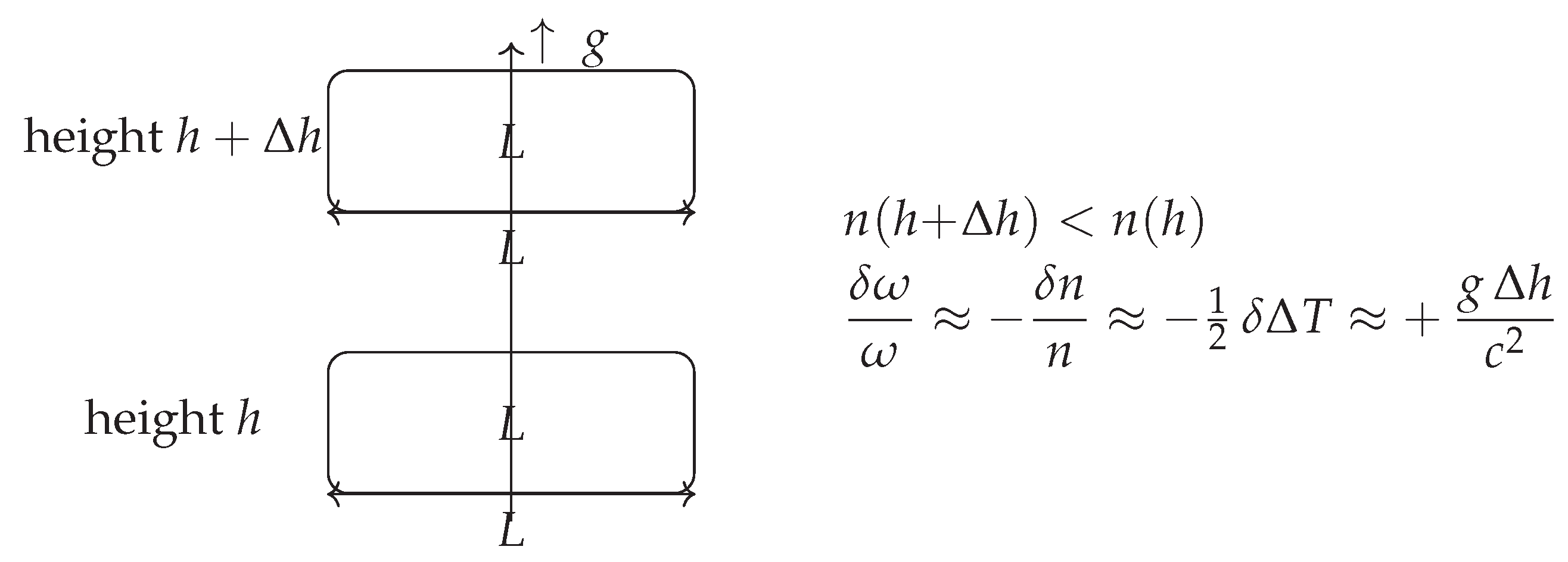
- Cavity frequency shift (local test).
For a rigid cavity of proper length L at position , the mth longitudinal mode obeys
consistent with the gravitational redshift: moving the cavity upward by on Earth gives (since decreases with altitude)[19]. The setup is sketched in Figure 7.
- Fiber/space link Shapiro test (field test).
9.5. Additivity with Ordinary Media (Index Bookkeeping)
If light also traverses a material medium with refractive index , then to first order in
so gravitational and material contributions factor multiplicatively (additively in ). This is useful for metrology setups (fibers, cells) where one separates material dispersion from TD contributions.
9.6. Gauge and Charge Conservation
Equations (58)–(60) preserve charge conservation exactly:
since is time–independent in the quasistatic TD approximation. Gauge freedom of the four–potential is unchanged; TD does not alter EM gauge symmetry.
9.7. Scope and Limits
The medium picture (57) assumes (i) a static or slowly varying TD background ( during measurement), and (ii) weak fields () for the isotropic index. Near horizons or in strongly curved regions one should use the full with the appropriate (the bridge reproduces the GR geometric–optics limit exactly).
Figure 7.
Cavity redshift as an index effect. Raising a rigid cavity by changes and shifts the mode frequency according to Eq. (66), consistent with the gravitational redshift.
Figure 7.
Cavity redshift as an index effect. Raising a rigid cavity by changes and shifts the mode frequency according to Eq. (66), consistent with the gravitational redshift.
10. Quantum–Ready Observables (No New Degrees of Freedom)
In this section we treat as a classical background (bridge regime with ) and quantize matter/EM fields on top of it, exactly as in QFT on curved spacetime. Quantum phases accrue from proper time with (Eq. (8)); this yields immediate, testable predictions for clocks, interferometers, and cavities without introducing a new propagating gravitational mode.
10.1. Universal Phase from Proper Time
For any stationary energy eigenstate with local energy E, the quantum phase along a worldline is
so the TD contribution to the differential phase between two paths is
In the nonrelativistic limit, taking and with Newtonian potential reproduces the standard gravitational phases[1].
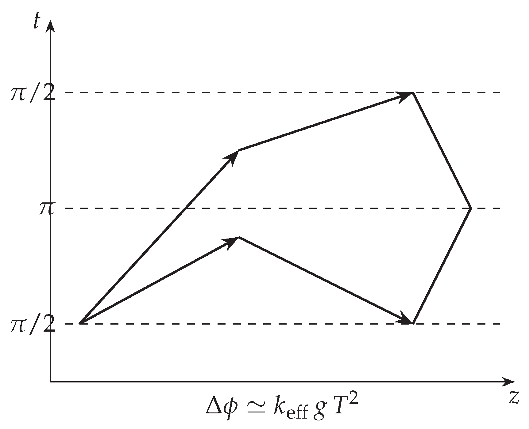
10.2. Atom Interferometers (Mach–Zehnder Class)
Consider two branches separated vertically in a uniform field (approximately constant ). Using Eq. (71) with and ,
the usual Kasevich–Chu result ( two-photon momentum transfer; T pulse separation)[29,30]. Thus TD predicts the same inertial response as GR/Newton in the bridge regime; the equivalence principle holds at this order. Our Mach–Zehnder geometry is shown in Figure 8.
10.3. Quantum Clocks (Ramsey and Comparisons)
10.4. Optical Cavities and Photons
For a rigid cavity of proper length L at location , the longitudinal resonance is
so a small change produces
as stated in Sec. 9. Raising the cavity by gives (since decreases with altitude)[19].
10.5. Matter–Wave Gravimetry from
10.6. Optional: Stochastic Slow–Time Noise (Bounds Only)
If one phenomenologically allows tiny, stationary fluctuations around the static background (still no new propagating DoF), the phase in Eq. (70) becomes stochastic. Defining the one-sided PSD and a temporal weighting window (interferometer or Ramsey sequence),
with the Fourier transform of w. Observed contrasts then bound . This is an optional TD phenomenology; in the main text we set .
10.7. Gauge, Locality, and Consistency
- Local Lorentz: In the bridge regime () local Lorentz invariance holds; N rescales coordinate time but does not alter local light cones.
- No extra graviton: We do not add a scalar gravitational wave; is a reparameterization of the lapse. Quantum tests here probe the background slow–time field, not a new radiation channel[1].
Figure 8.
Mach–Zehnder atom interferometer in a uniform field. The TD background enters phases via and , yielding the standard signal (Eq. (72)).
Figure 8.
Mach–Zehnder atom interferometer in a uniform field. The TD background enters phases via and , yielding the standard signal (Eq. (72)).
10.8. Takeaway
TD turns quantum sensors into direct probes of the slow–time field: phases scale with integrals of (or its gradients), while spectra and contrasts can, in principle, bound any tiny stochastic component of . In the frozen baseline, all predictions reduce to those of GR in the tested regimes; the framework is thus ready for near–term quantum tests without additional assumptions. Key quantum observables and their leading TD dependences are collected in Table 5.
11. Cosmology in TD
In homogeneous cosmology the TD baseline may drift slowly in time,
with small and (on Hubble times) nearly constant. In the pure baseline limit (no matter/radiation), TD gives de–Sitter–like expansion
More generally, when matter and radiation are present and the baseline drift is uniform in space, TD is observationally equivalent to GR with a (possibly mild) time–dependent cosmological term
11.1. A Minimal One–Parameter Extension
To test for tiny departures from CDM, adopt
so that
Define the present–day density parameters (so ). Then
which reduces to CDM when .
11.2. Distances and Horizons
11.3. Bound vs. Unbound: the TD Turnaround Scale
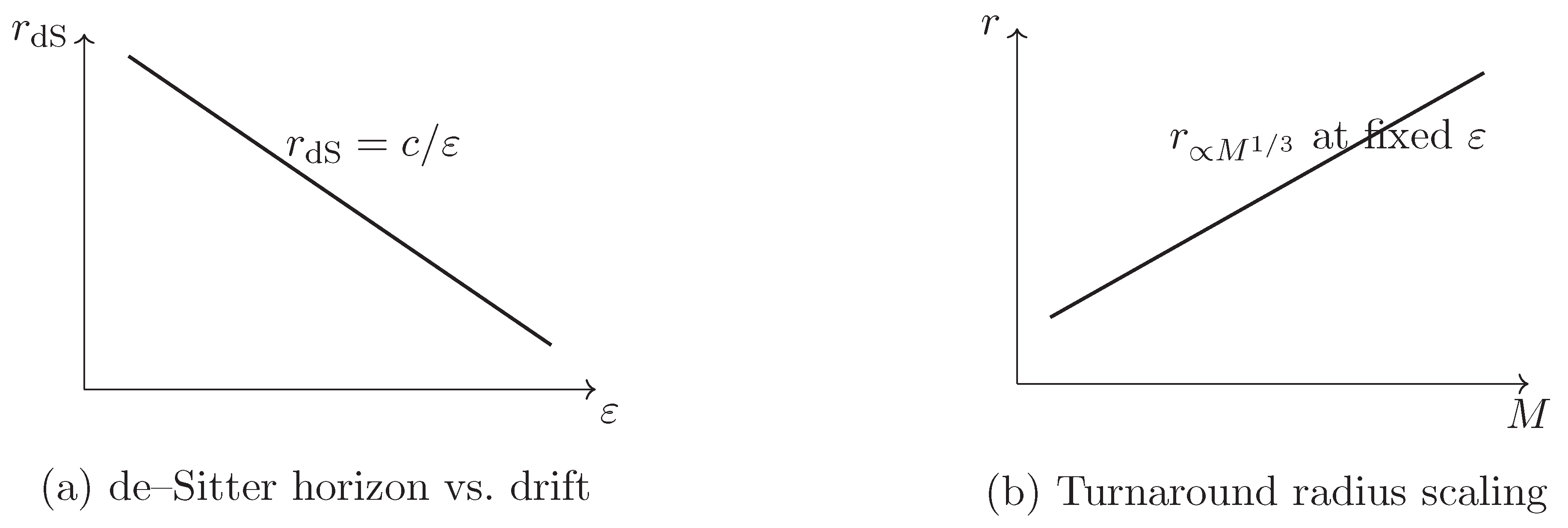
Balancing the inward slow–time gradient pull against the outward baseline push gives the TD turnaround radius
inside which structures can remain bound (quasi–static) and outside which the uniform drift dominates. This mirrors the CDM turnaround scale[32] and provides a direct, falsifiable link from the clock drift to group/cluster environments.
11.4. Growth of Structure (Linear Regime)
Writing derivatives with respect to , the linear growth factor satisfies
with and from Eq. (85) via [33]. In the TD extension the effective dark–energy term keeps (pressure ) but its amplitude varies as ; growth–index parameterizations remain approximately valid with small shifts controlled by p through [34].
11.5. Observational Program (Concise)
- Horizon scale: Use Eq. (89) for intuition and consistency checks; it sets the limiting comoving scale for causal influence in a drift–dominated epoch.
11.6. Limits and Degeneracies
Small p is partially degenerate with reparameterizations and with . Joint fits should either (i) fix curvature to a Planck–consistent prior and report p, or (ii) explore jointly and quote marginalized bounds[36]. By construction recovers CDM exactly.
11.7. Genesis in TD (One Paragraph)
In TD the universe begins when the clock turns on (). An early phase with large, nearly constant smooths the universe (inflation–like), then decays and reheats into fields; later, a tiny residual drives the present acceleration. This reframes the GR singularity as a pre–clock boundary () rather than a curvature blow–up, and ties the entire expansion history to the single causal rate .
- Key equations (for quick reference)
Figure 9.
Cosmology in TD: key scalings. (a) The horizon scale is set by the baseline drift, . (b) The TD turnaround radius scales as for fixed , matching the CDM expression with .
Figure 9.
Cosmology in TD: key scalings. (a) The horizon scale is set by the baseline drift, . (b) The TD turnaround radius scales as for fixed , matching the CDM expression with .
12. Experiments and Observational Program
This section turns the TD relations into concrete measurements; representative magnitudes are listed in Table 6. We split the program into (i) laboratory/near–Earth tests that probe and its gradient directly, (ii) astronomical tests of photon propagation, and (iii) cosmological fits that constrain a possible clock drift .
12.1. Laboratory and Near–Earth (Direct Mapping)
- Clock networks (primary).
Deploy identical or cross–calibrated clocks at ; measure frequency ratios with two–way links. Using Eq. (21),
A vertical pair separated by gives, from Eq. (24),
consistent with state–of–the–art optical clocks and satellite comparisons[19,20,21]. Deliverable: a 2D map of (Dirichlet/Neumann reconstruction; Eq. (23)), and a direct test that matches local gravimetry.
- Atom interferometers.
In a Mach–Zehnder geometry, the phase follows Eq. (72): . Operate the interferometer on multiple baselines to sample spatially; compare to classical gravimeters and the clock–inferred field[29,30].
- Cavity frequency shifts.
A rigid cavity of proper length L moved by satisfies Eq. (76): (since decreases with altitude). Use: photon–based check of the clock result with different systematics[19].
- Shapiro on fiber/microwave links.
Route a phase–stable link along a path past known mass distributions; the additional delay is [Eq. (30)]. Design: pick routes with strong known potentials (mountain shoulders, urban towers); compare with predictions from reconstructed by the clock grid.
- Source inversion (optional).
With a bounded domain , solve Eq. (11) to estimate from the reconstructed map. Caveat: boundary modeling and noise regularization dominate errors.
12.2. Astronomical Propagation Tests
- Solar–system timing.
Radio/laser ranging with impact parameter yields the one–way Shapiro delay s (Sec. 4), consistent with Cassini tests[8,9]. This directly matches Eq. (30) with .
- Light deflection and time delays.
12.3. Cosmology: Distances, Growth, and Key Scales
- Distance ladder (primary).
Fit the one–parameter TD extension via in Eq. (85). Use SNe Ia luminosity distances , BAO (, ), and cosmic chronometers ; report p (Eq. (83)) with uncertainties and the (CDM) limit[14,15,16,35,36].
- Growth and RSD.
Use the linear growth equation Eq. (91) to predict and compare with redshift–space distortion data; check distance/growth consistency[34,36].
- Turnaround and splashback radii.
12.4. How to Report (Falsifiable Targets)
- Local gradient law: publish maps and verify within errors over the domain. Any systematic, coordinate–independent violation falsifies TD (or the weak/quasistatic approximation).
- Cosmology: report p with a clear prior on ; if p is consistent with 0, give a 95% upper bound. Publish comparisons with explicit environment systematics.
12.5. Systematics and Error Budgets (Checklist)
- Clocks/links: Allan deviation, transfer noise, temperature/strain of fibers, tidal loading, atmospheric delay (for free–space).
- Gravimetry: instrument tilt, vibration, Coriolis effects for atom interferometers; co–location with clocks for common–mode rejection.
- Cavities: thermoelastic and refractive changes in materials; local acceleration sensitivity (mount design).
- Timing/propagation: ephemerides, plasma dispersion, tropospheric delay; impact parameter uncertainties.
- Cosmology: calibration systematics in SN Ia; BAO reconstruction choices; chronometer stellar population modeling; RSD velocity bias; curvature degeneracy with p.
Table 6.
Compact targets and typical magnitudes for near-term tests. Weak-field optical entries reduce to standard GR results for a point mass (Shapiro delay [8]; solar-limb deflection [4,10]).
| Observable | Leading dependence | Typical scale |
|---|---|---|
| Clock redshift (1 m) | per m | |
| AI phase | e.g. , s | |
| Cavity shift | same sign/magnitude as clock shift | |
| Shapiro (solar graze) | s (one–way) | |
| Deflection (Sun limb) | ||
| Turnaround scale | Mpc for | |
| dS horizon | today |
12.6. Roadmap and Milestones
- Local: produce a campus–scale map from clocks; publish the gradient–law closure with a joint clock/AI/cavity dataset.
- Propagation: demonstrate a controlled Shapiro measurement on a terrestrial link and match the line integral of reconstructed .
- Cosmology: release a baseline p fit to SN Ia+BAO+chronometers (flat prior on curvature); follow with a joint exploration and growth cross–checks.
- Astro scale: publish vs. splashback comparisons for a clean cluster subsample with environment controls.
12.7. What Would Decisively Falsify TD (in this Paper’s Scope)
- A robust, coordinate–independent failure of in the weak, quasistatic regime.
- A systematic mismatch between measured delays/deflections and the line integrals using the same mass model.
- Cosmology requiring p far from zero while distances and growth cannot be reconciled within Eq. (85).
13. Objections and Replies
This section anticipates common critiques and answers them within the scope and equations of this paper.
O1. “Isn’t just the ADM lapse in disguise?”
Reply. Yes—in the bridge regime we set (Eq. (47)). The novelty is operational and causal: is defined by clock ratios (Sec. 3), and TD posits an explicit space–growth clock as the cause that, when frozen (), reproduces the GR representation. No extra degrees of freedom are introduced.
O2. “Then you added a scalar graviton, right?”
Reply. No. The lapse is non-dynamical in GR; reparameterizing it by does not add a propagating mode. The constraint algebra and DoF are unchanged (Sec. 8). Linearization yields the usual two tensor polarizations at speed c, with no extra scalar GW.
O3. “Local Lorentz invariance?”
Reply. Preserved. In the bridge regime (Eq. (16)); N rescales coordinate time, not light cones. All local measurements see c; optical effects arise through the coordinate index (Secs. 5, 9).
O4. “Equivalence principle and composition dependence?”
O5. “ constant would change physics.”
O6. “Why must ?”
Reply. Operationally, clocks do not tick faster than the baseline with normal matter sourcing. Mathematically, with asymptotic flatness and positive active density, the elliptic maximum principle gives outside horizons, hence (Sec. 2). The limit is a black boundary (), not the pre-clock state (Sec. 6).
O7. “Isn’t this just the Newtonian potential ?”
Reply. In the weak field , so TD reduces to Newton+optics. Beyond that, is the full lapse reparameterization ; strong fields and horizons are handled by N directly, not by a single scalar potential.
O8. “Gauge/coordinate dependence of ?”
Reply. The definition uses only clock ratios and spatial differences measured along a physical baseline (Sec. 3); is an observable scalar under our stated assumptions (static exterior, chosen slicing). Coordinates are bookkeeping for maps and integrals.
O9. “Energy–momentum conservation and Bianchi identities?”
Reply. In the bridge regime the field equations and constraints are those of GR (Sec. 8); holds. In the weak, static limit our Poisson law (Eq. (11)) is the standard GR limit and is consistent with mass continuity.
O10. “Rotation (Kerr), frame dragging?”
Reply. TD maps the lapse via while leaving the shift and spatial metric untouched. Frame dragging resides in ; Kerr observables (ISCO, lensing, redshift) are inherited slice-by-slice from GR (Sec. 8).
O11. “Gravitational waves?”
Reply. Two tensor polarizations at speed c; no extra scalar mode (Sec. 8). This is consistent with multi-messenger bounds on GW speed and polarization content.
O12. “Electromagnetic back-reaction is negligible, so why include it?”
Reply. Conceptually essential yet quantitatively tiny in labs (Sec. 7). In extreme astrophysics (e.g. magnetars) it can be a principled correction to baryonic sourcing. Propagation vs. sourcing are cleanly separated: for optics; for back-reaction.
O13. “Strong lensing/black hole shadow: does the index picture break?”
Reply. The isotropic-medium picture is a weak-field shorthand. Near horizons one should use the full with the appropriate (bridge to GR) to compute null geodesics. In that limit TD reproduces GR shadow/lensing predictions.
O14. “Cosmology: is distinguishable from ?”
Reply. TD’s drift yields with but varying amplitude (Sec. 11). Small p is partially degenerate with and curvature; we recommend reporting p with a clear curvature prior, then a joint analysis (Sec. 11).
O15. “Turnaround radius is crude.”
Reply. It is a zeroth-order, falsifiable scale from first principles: (Eq. (90)). Environment, tides, and infall bias the mapping to splashback/zero-velocity surfaces; we treat those as nuisances, not a failure of the anchor.
O16. “Is TD just a conformal rephrasing?”
Reply. No. TD fixes a physical normalization () and ties observables to an operational scalar measured by clocks. The bridge is a field redefinition of the lapse (no new DoF), but the cause—a real baseline clock with possible tiny drift —is additional physical content tested in Secs. 11–12.
O17. “Inside horizons / singularities?”
Reply. This paper’s domain is the exterior (). Horizons are surfaces; interior evolution requires a different foliation, as in GR. TD reframes the initial singularity as a pre-clock boundary () rather than curvature blow-up; cosmological claims here are limited to homogeneous drift (Sec. 11).
O18. “Can (faster clocks) occur?”
Reply. Not with normal (positive) energy under our assumptions. would require exotic matter or nonstandard slicings we do not consider. With asymptotic flatness and positive active density we have (Eq. (17)).
O19. “Are your laboratory targets realistic?”
Reply. Yes. Vertical clock redshifts at the /m level, AI phases , cavity shifts matching , and controlled Shapiro delays on engineered links are within current or near-term technology (Sec. 12). The program is falsifiable: a robust failure of would refute the weak/quasistatic TD mapping.
O20. “Scope creep: where are the full dynamics?”
Reply. By design, this paper restricts to quasistatic, weak fields for clarity and testability. The full action-level bridge and constraint structure are delegated to the companion note (Sec. 8 pointer). None of the weak-field predictions used here require additional dynamics beyond the GR bridge.
14. Limitations and Scope
This paper is intentionally conservative. We isolate the minimal, operational content of TD in regimes where it can be tested cleanly, and we point to a companion bridge note for action-level details. Below we list the main assumptions, approximations, and exclusions.
14.1. Assumptions used Throughout
- Frozen baseline in the bridge regime: we impose the Normalization Axiom (Eq. (16)) whenever we compare with GR/PPN and laboratory data.
- Static exterior and chosen slicing: is defined operationally for static observers (Sec. 3). Inside horizons () we do not use ; a different foliation would be required.
- Spatially uniform drift for cosmology: when discussing (Sec. 11) we assume it is homogeneous and small on Hubble timescales; spatial variations of S are not considered.
14.2. Approximations Specific to Observables
- Optics as an isotropic medium: the index model (Sec. 5) is a weak-field shorthand. Near horizons or in strong lensing we appeal to the full bridge ( with the appropriate ).
- Source law: the Poisson form (Eq. (11)) is the static, weak-field limit using the active density . Nonlinear and time-dependent terms , are outside our scope.
- Quantum tests: Sec. 10 quantizes matter/EM on a classical background (); we do not introduce a new gravitational degree of freedom or a propagating wave.
14.3. Cosmology-Specific Caveats
- One-parameter extension: the model for (Eq. (84)) is a minimal ansatz; it is not a claim about the ultraviolet origin of .
- Degeneracies: small p is partially degenerate with curvature and ; reported bounds must specify priors (Sec. 11).
- Turnaround scale: (Eq. (90)) is a zeroth-order anchor. Environment, tides, and infall shift observed splashback/zero-velocity radii; these are treated as nuisances, not a failure of the scaling.
14.4. What we do not Claim Here
- No new radiative gravitational mode; no modification of GW polarizations or speed.
- No alternative to GR in the strong-field dynamical regime; we rely on the bridge in those cases.
- No microphysical model for the “clock” or for the genesis of ; Sec. 11 gives a phenomenological narrative only.
- No treatment of rotating/charged horizons beyond the statement that the lapse mapping recovers Kerr–Newman results slice-by-slice.
14.5. Domain of Validity (One-Line Summary)
The results in Secs. 4–12 are intended for static/weak fields outside horizons with (bridge), plus a homogeneous, tiny cosmological drift that is tested against distance and growth data.
15. Conclusions
We have presented a native formulation of Temporal Dynamics in which a universal space–growth clock provides the cause, and GR emerges as the representation when the baseline is frozen (). A single, operational scalar—the slow–time field —controls both kinematics and optics. In the weak, quasistatic regime,
reproduce Newton’s law, gravitational redshift, Shapiro delay, and light deflection; horizons are the surfaces calibrated by .
Electromagnetism on a TD background separates cleanly into propagation (rays/indices) and sourcing (active density), while quantum-ready observables follow directly from proper-time phases without adding new gravitational degrees of freedom. On cosmological scales, a tiny, homogeneous drift of the baseline, , maps to an effective , yielding a one-parameter extension of CDM with falsifiable signatures in distances, growth, and the turnaround scale .
The accompanying experimental/observational program is straightforward: map with clock networks and verify the gradient law against gravimetry; test the optical dictionary on engineered links and lensing; and fit the cosmological extension with SN Ia, BAO, and , cross-checking growth. Any robust, coordinate-independent failure of these relations would falsify the framework in its stated domain.
- Future directions.
(i) Present the full action-level bridge and constraint algebra; (ii) extend strong-field applications (Kerr, shadows, ringdowns) within the TD dictionary; (iii) develop a microscopic model for the clock and early-time ignition consistent with ; (iv) execute the cosmology fits and laboratory maps proposed here.
- Takeaway.
TD articulates a cause-level picture (a real clock) whose frozen-baseline representation is GR, packages the weak-field phenomenology into one operational scalar , and offers near-term, falsifiable tests from laboratories to the Hubble scale.
Author Contributions
CRediT taxonomy. Roles follow the CRediT (Contributor Roles Taxonomy) standard. Ogaeze Onyedikachukwu Francis (O. O. Francis): Conceptualization; Methodology; Formal analysis; Investigation; Validation; Writing—original draft; Writing—review & editing; Visualization.
Funding
This work received no specific grant from any funding agency in the public, commercial, or not-for-profit sectors.
Data Availability Statement
No new data were generated or analyzed in this study. All derivations and numerical estimates are contained in the main text and appendices; any auxiliary scripts used to produce figures will be made available upon reasonable request.
Acknowledgments
The author thanks one early reader for brief comments on clarity. This work is primarily the author’s, and it builds on the existing literature in weak-field tests of GR, optical-clock metrology, gravitational lensing and time-delay formalisms, and cosmological distance–growth analyses; those contributions are acknowledged through citations throughout the text. Any remaining errors are the author’s responsibility.
Conflicts of Interest
The author declares no competing interests.
Appendix A. Units and Normalizations
- Baseline (clock): , units m s−1. In the bridge regime: Normalization Axiom (Eq. (16)).
- Optics: (Eq. (12)); Fermat functional .
- Sourcing (weak/static): (Eq. (11)).
- Horizon calibration: black boundary at ; diameter (Eq. (13)).
- Sign conventions: ∇ is the flat spatial gradient in the weak field; points outward so .
Appendix B. Bridge: Action Sketch and Constraints (Details)
In ADM variables ,
Define so and . The lapse variation in TD variables is the GR Hamiltonian constraint times a nonzero factor:
Momentum constraints (variation of ) and evolution equations (variation of ) are unchanged; the constraint algebra and DoF therefore match GR.
- Weak/static limit to the Poisson law.
Linearize around Minkowski with , , . The Hamiltonian constraint reduces to
which is Eq. (11).
Appendix C. PPN Snapshot (β = γ = 1)
With (Newtonian potential ) and ,
so . The light deflection and Shapiro delay follow from the index and Fermat’s principle; perihelion precession reduces to the GR value with . No deviations appear in the tested weak field.
Appendix D. Kerr Note: Lapse and ΔT
In Boyer–Lindquist coordinates ( for brevity) define
The 3+1 lapse for the usual Kerr foliation is
The shift has only a component ; TD leaves and unchanged. The black boundary occurs where , i.e. at . In the Schwarzschild limit (), and , matching the weak field and the horizon calibration.
Appendix E. Gravitational Waves: Linearization
Linearize around Minkowski with , , and with . The lapse perturbation is non-propagating (it enforces the Hamiltonian constraint). In transverse–traceless gauge the spatial metric perturbation satisfies
with two tensor polarizations and no scalar mode, consistent with the bridge statement in Sec. 8.
Appendix F. Back-of-the-Envelope Numbers
Constants: m s−1, m3 kg−1 s−2.
Earth: kg, m.
- Earth surface slow–time: .
- Clock redshift per meter: .
- Solar limb deflection: .
- Solar Shapiro (grazing, one–way): s.
- Magnetar EM density: T J m−3, kg m−3.
- Cosmic drift scales: with s−1, de Sitter horizon m ( Gpc). Equivalently, using , .
-
Turnaround scale: givesSun: m ( pc), Milky Way (): Mpc, Rich cluster (): Mpc.
Appendix G. Data-Fit Recipe for the TD Cosmology Parameter p
Inputs
SN Ia distances ; BAO ; chronometer ; (optional) RSD .
Model
Likelihood (schematic)
Reporting
Quote p with a stated prior on ; provide (CDM) as a nested model check. For TD key scales, report using Eq. (90) with .
Appendix H. Notation Table
| Symbol | Meaning | Units |
| c | Invariant local light speed; normalization baseline in bridge regime | m s−1 |
| G | Newton’s gravitational constant | m3 kg−1 s−2 |
| Space–growth clock (baseline speed) | m s−1 | |
| Baseline fractional rate (“clock drift”) | s−1 | |
| Slow–time field () | — | |
| N | ADM lapse, | — |
| ADM shift (frame dragging / rotation) | m s−1 | |
| Spatial 3-metric on the slice | — | |
| Effective refractive index, | — | |
| Gravitational acceleration, | m s−2 | |
| v | Kinematic speed, (quasistatic) | m s−1 |
| Energy density divided by | kg m−3 | |
| Principal pressures | Pa | |
| Active density, | kg m−3 | |
| Newtonian potential (weak field: ) | m1 s−2 | |
| Hubble parameter | s−1 | |
| Scale factor | — | |
| Effective cosmological term, | m−2 | |
| Normalized expansion rate, | — | |
| Present-day density parameters | — | |
| Comoving, transverse comoving, luminosity, angular-diameter distances | m | |
| de Sitter (cosmological) horizon, | m | |
| TD turnaround scale, | m | |
| Schwarzschild radius, | m | |
| Black-boundary diameter, | m | |
| b | Impact parameter (lensing/deflection) | m |
| Two-photon momentum transfer (atom interferometry) | m−1 | |
| T | Pulse separation time in AI / interrogation time | s |
| Clock frequency | Hz | |
| Angular frequency | s−1 | |
| EM energy density; mass density | J m−3; kg m−3 |
References
- Will, C.M. The Confrontation between General Relativity and Experiment. Living Reviews in Relativity 2018, 21, 3. [CrossRef]
- Carroll, S.M. Spacetime and Geometry: An Introduction to General Relativity; Addison-Wesley, 2004.
- Wald, R.M. General Relativity; University of Chicago Press, 1984.
- Schneider, P.; Ehlers, J.; Falco, E.E. Gravitational Lenses; Springer, 1992.
- Francis, O.O. Temporal Dynamics: For Space–Time and Gravity. Preprints 2025. Preprint, . [CrossRef]
- Arnowitt, R.; Deser, S.; Misner, C.W. The Dynamics of General Relativity. In Gravitation: An Introduction to Current Research; Witten, L., Ed.; Wiley, 1962. Reprinted: Gen. Relativ. Gravit. 40, 1997–2027 (2008).
- Gourgoulhon, E. 3+1 Formalism and Bases of Numerical Relativity, 2007, [gr-qc/0703035]. arXiv preprint.
- Shapiro, I.I. Fourth Test of General Relativity. Physical Review Letters 1964, 13, 789–791. [CrossRef]
- Bertotti, B.; Iess, L.; Tortora, P. A Test of General Relativity Using Radio Links with the Cassini Spacecraft. Nature 2003, 425, 374–376. [CrossRef]
- Dyson, F.W.; Eddington, A.S.; Davidson, C. A Determination of the Deflection of Light by the Sun’s Gravitational Field. Philosophical Transactions of the Royal Society A 1920, 220, 291–333.
- Abbott, B.P.; others (LIGO Scientific Collaboration.; Collaboration), V. GW170817: Observation of Gravitational Waves from a Binary Neutron Star Inspiral. Physical Review Letters 2017, 119, 161101. [CrossRef]
- Abbott, B.P.; et al. Gravitational Waves and Gamma-Rays from a Binary Neutron Star Merger: GW170817 and GRB 170817A. The Astrophysical Journal Letters 2017, 848, L13. [CrossRef]
- Francis, O.O. Temporal Dynamics as Time-First General Relativity. Preprints 2025. Preprint, . [CrossRef]
- Riess, A.G.; et al. Observational Evidence from Supernovae for an Accelerating Universe and a Cosmological Constant. The Astronomical Journal 1998, 116, 1009–1038. [CrossRef]
- Perlmutter, S.; et al. Measurements of Ω and Λ from 42 High-Redshift Supernovae. The Astrophysical Journal 1999, 517, 565–586. [CrossRef]
- Eisenstein, D.J.; et al. Detection of the Baryon Acoustic Peak in the Large-Scale Correlation Function of SDSS Luminous Red Galaxies. The Astrophysical Journal 2005, 633, 560–574. [CrossRef]
- Pound, R.V.; Rebka, G.A. Apparent Weight of Photons. Physical Review Letters 1960, 4, 337–341. [CrossRef]
- Pound, R.V.; Snider, J.L. Effect of Gravity on Nuclear Resonance. Physical Review Letters 1965, 13, 539–540. [CrossRef]
- Chou, C.W.; Hume, D.B.; Koelemeij, J.C.J.; Wineland, D.J.; Rosenband, T. Optical Clocks and Relativity. Science 2010, 329, 1630–1633. [CrossRef]
- Delva, P.; et al. Test of the Gravitational Redshift with Stable Clocks in Eccentric Orbits. Physical Review Letters 2018, 121, 231101. [CrossRef]
- Herrmann, S.; et al. Test of the Gravitational Redshift with Galileo Satellites in an Eccentric Orbit. Physical Review Letters 2018, 121, 231102. [CrossRef]
- Poisson, E.; Will, C.M. Gravity: Newtonian, Post-Newtonian, Relativistic; Cambridge University Press, 2014.
- Francis, O.O. Essence Dynamics: Essence Interactions, Applications and Reality. Part II. Preprints 2024. Preprint, . [CrossRef]
- Ashby, N. Relativity in the Global Positioning System. Physics Today 2003, 55, 41–47. [CrossRef]
- Collaboration, E.H.T. First M87 Event Horizon Telescope Results. I. The Shadow of the Supermassive Black Hole. The Astrophysical Journal Letters 2019, 875, L1. [CrossRef]
- Jackson, J.D. Classical Electrodynamics, 3rd ed.; Wiley, 1998.
- Gordon, W. Zur Lichtfortpflanzung nach der Relativitätstheorie. Annalen der Physik 1923, 377, 421–456.
- Plebański, J. Electromagnetic waves in gravitational fields. Phys. Rev. 1960, 118, 1396–1408.
- Kasevich, M.; Chu, S. Atomic interferometry using stimulated Raman transitions. Phys. Rev. Lett. 1991, 67, 181–184.
- Cronin, A.D.; Schmiedmayer, J.; Pritchard, D.E. Optics and interferometry with atoms and molecules. Rev. Mod. Phys. 2009, 81, 1051–1129.
- Hogg, D.W. Distance measures in cosmology. arXiv:astro-ph/9905116 1999.
- Pavlidou, V.; Tomaras, T.N. Where the world stands still: turnaround radius in ΛCDM. JCAP 2014, 09, 020.
- Dodelson, S. Modern Cosmology; Academic Press, 2003.
- Linder, E.V. Cosmic Growth History and Expansion History. Physical Review D 2005, 72, 043529. [CrossRef]
- Moresco, M.; et al. Improved Constraints on the Expansion Rate of the Universe up to z ∼ 1.1 from the Spectroscopic Evolution of Cosmic Chronometers. JCAP 2012, 2012, 006. [CrossRef]
- Collaboration, P. Planck 2018 results. VI. Cosmological parameters. A&A 2020, 641, A6.
| 1 | One can also view (29) as the statement that phases counted per unit proper time are invariant, while coordinate time dilates by . The index n governs propagation below. |
Figure 4.
Ray picture in the index-of-time medium. Gradients of (set by ) deflect light and produce the Shapiro delay; both recover the standard GR values in the weak field.
Figure 4.
Ray picture in the index-of-time medium. Gradients of (set by ) deflect light and produce the Shapiro delay; both recover the standard GR values in the weak field.
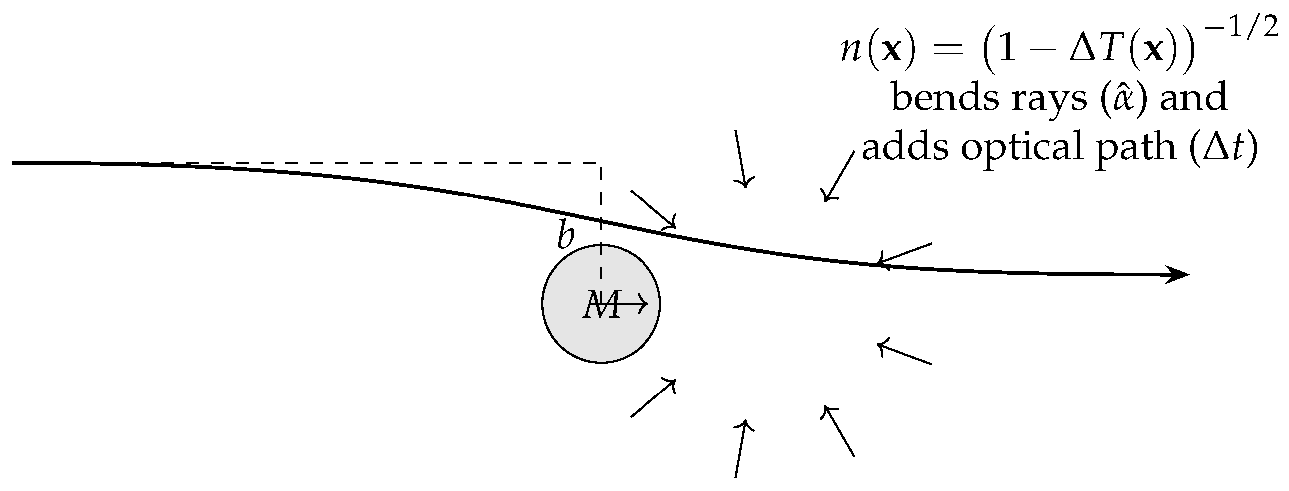
Table 2.
Operational pipeline for mapping . The inputs are instrument readings and transfer links; outputs are the field, its gradient, and (optionally) source inversions.
Table 2.
Operational pipeline for mapping . The inputs are instrument readings and transfer links; outputs are the field, its gradient, and (optionally) source inversions.
| Step | Input/Method | Primary output |
|---|---|---|
| Clock grid | , stable links[24] | Frequency field |
| Ratios | Neighbor pairs | Common–mode rejection |
| Gradients | Fit | (Eq. (20)) |
| Field | Path integral / PDE | (Eqs. (22), (23)) |
| Gravity | Eq. (21) | |
| Source (opt.) | Eq. (11) |
Table 3.
Minimal TD→observable dictionary in the quasistatic, weak–field regime () with the Normalization Axiom . The Shapiro delay and lensing expressions reduce to the standard GR results [4,8].
| Quantity | TD expression (weak field) |
|---|---|
| Gravitational acceleration | |
| Gravitational redshift | |
| Shapiro time delay | [8] |
| Light deflection (small angle) | [4] |
| Effective index of vacuum |
Table 5.
Quantum-ready observables and their leading TD dependences in the bridge regime () and weak, quasistatic fields (). Phases come from proper time with ; the Shapiro entry reduces to the standard GR expression [8].
Table 5.
Quantum-ready observables and their leading TD dependences in the bridge regime () and weak, quasistatic fields (). Phases come from proper time with ; the Shapiro entry reduces to the standard GR expression [8].
| Observable | Leading TD dependence |
|---|---|
| Atom interferometer phase | |
| Clock comparison (Ramsey) | |
| Cavity frequency shift | |
| Photon time transfer (Shapiro) |
Disclaimer/Publisher’s Note: The statements, opinions and data contained in all publications are solely those of the individual author(s) and contributor(s) and not of MDPI and/or the editor(s). MDPI and/or the editor(s) disclaim responsibility for any injury to people or property resulting from any ideas, methods, instructions or products referred to in the content. |
© 2025 by the authors. Licensee MDPI, Basel, Switzerland. This article is an open access article distributed under the terms and conditions of the Creative Commons Attribution (CC BY) license (http://creativecommons.org/licenses/by/4.0/).
Copyright: This open access article is published under a Creative Commons CC BY 4.0 license, which permit the free download, distribution, and reuse, provided that the author and preprint are cited in any reuse.


