
Submitted:
27 November 2025
Posted:
01 December 2025
You are already at the latest version
Abstract
Neighborhood variations in depression, an important aspect of the overall mental health burden, have been linked both to environmental context (e.g. area crime, neighborhood cohesion), and to area socio-demographic composition. Previous models seeking to explain such spatial variations in mental health, such as those based on Bayesian disease mapping, follow a standard approach defined by: spatially stationary effects of area predictors; predictor effects neglecting potential spatial spillover; and a spatially structured residual to account for unmodelled spatial dependencies. In a study of depression incidence in England neighborhoods, we consider the gains from an alternative strategy, allowing nonstationary environmental impacts; spillover effects of environmental factors, and a non-stationary spatial intensity. We focus particularly on impacts of socio-behavioral environments, namely neighborhood cohesion and crime. We find these to be major influences on neighborhood depression incidence, and also find major gains in model performance by explicitly considering non-stationarity and spillovers. Allowing context heterogeneity, varying spatial intensity and spillover are shown to enhance the impacts of socio-behavioral environments on depression incidence, and such findings have broader relevance to disease mapping regression.
Keywords:
depression
; neighborhood
; crime
; collinearity
; cohesion
; urbanicity
; heterogeneity
; spillover
; non-stationarity
1. Introduction
Neighborhood variations in depression are an important aspect of the overall mental health burden, and typically co-morbid with other mental illnesses such as psychosis. Such variations, or those in common mental disorders more generally, have been explored relatively little, but available studies [1,2] show major influences of area socio-demographic composition, ethnic mix, and contextual environmental factors, such as area crime, urbanicity, and neighborhood social cohesion. Meta-analysis [3] shows significant impacts of neighborhood on depressive symptoms, controlling for individual attributes (such as age, income, and ethnicity). Neighborhood influences are relevant to spatial variations in other mental health outcomes [4,5].
We focus in the present study on such place effects, namely the impacts of socio-behavioral environments. In particular, we consider the role in explaining neighborhood depression of cohesion and crime [6,7], and how these impacts operate spatially. It has been argued [8] that existing studies of depression over-emphasize the relevance of socio-economic composition and neglect the role of contextual neighborhood characteristics, both objective and subjective (e.g. actual and perceived crime levels). Thus [8, page 43] states “both failure to control for nesting of people within geographic space [..], and an almost exclusive focus on neighborhood socioeconomic status [..] limit understanding of the ways in which neighborhood characteristics influence depressive symptoms”.
1.1. Full Accounting for Spatial Effects
As well as taking fuller account of health impacts linked to socio-environmental contexts, we also consider associated issues in appropriate modelling of spatial impacts. Models for spatial variations in mental health, such as those based on Bayesian disease mapping [9,10,11], follow the standard disease mapping approach [12,13], namely: spatially homogenous effects of area predictors; predictors defined without regard to possible spillover effects; and a spatially structured residual random effect to account for unmodelled spatial dependencies.
We instead here assess gains (statistical and substantive) from considering impacts of spatial structure and spatial dependence more comprehensively. This is done in three major ways.
First, we consider spatial spillovers in environmental influences. The importance of spillover is acknowledged in causal approaches to assessing impacts of neighborhood exposures [14]. It is also recognized in spatial linear regression methodologies, including regression on spatially lagged predictors, and known as spatial Durbin regression [15]. An example of these two approaches to overlap is provided in studies of pollution impacts by Giffin et al [16] using a causal method, and by Sarrias and Molina-Varas [17], using spatial Durbin regression.
Spillover may also characterize impacts of social environments (e.g. cohesion, crime), access environments (e.g. exercise access) and so on, as these are not defined spatially by the arbitrary administrative boundaries of the neighborhoods typically used in ecological disease studies. For example, residents living nearer neighborhood boundaries are likely to experience spillover effects of environmental levels in adjacent areas. Regarding neighborhood crime rates, Graif [18] mention that “despite the rapidly growing ecological-level evidence indicating geographic spillover effects on crime, research on neighborhood effects [..] has treated neighborhoods as if they were isolated islands, independent of their surroundings”.
On conceptual grounds spatial spillover would be anticipated as most relevant for contextual environmental influences. A compositional effect is inherently an effect of the socio-demography of the local population, whereas a contextual effect from environmental influences is spatially unbounded in impact, spilling over administrative boundaries.
Second, we explicitly consider context heterogeneity (spatial non-stationarity), particularly regarding environmental influences. As discussed in [19] p.112 “much of the observed spatial correlation in residuals that is frequently observed [..] applied to spatial data results from applying a global model to a non-stationary process”. Non-stationarity can often be summarized in terms of spatial regimes, defined by Vidoli and Benedetti [20] as “an aggregation of neighboring units that are homogeneous in functional terms or that share the same relationship between a dependent variable and some covariates”. These have been infrequently considered in spatial epidemiology, though see Sridharan et al [21] for an exception.
Non-stationarity in neighborhood depression has been analyzed using frequentist geographically weighted (GWR) regression [22,23]. Drawbacks with the usual application of GWR are mentioned by [24]. Here we use Bayesian approaches [25] to spatially varying coefficients (SVC) that have been shown to have advantages in analyzing spatial data. For example, these include full posterior summaries regarding spatial random effects and can also be applied with variances themselves treated as non-stationary.
Thus, we allow for variations in the precision of spatial random effects, both for spatially varying coefficients and the spatial residual. The study [26] considered such heteroscedasticity just for spatial residuals, because spatial effects may be inherently less variable in some parts of the overall region (domain) being considered. We extend this approach here to heteroscedasticity in SVC effects.
Under the conditional autoregressive (CAR) spatial random effects approach of Besag et al [27] commonly used in the standard model, spatial variability, as measured by a precision parameter, is assumed constant over the domain. This assumption may be restrictive for a large domain with many small areas. We accordingly use multiple precision parameters, expressing different intensities of spatial dependence in different sub-regions. We apply a penalized complexity prior [28] to varying precision parameters to prevent overfitting.
Heteroscedasticity in CAR spatial random effects has been considered before e.g. [29] but existing approaches may involve many weakly identified parameters. Spatial volatility models are quite widely applied in spatial econometric applications using simultaneous autoregressive (SAR) models applied to continuous responses e.g. [30] under a linear normal assumption. However, these methods do not transfer straightforwardly to geographic disease applications, typically with count responses.
1.2. Depression Incidence in English Neighborhoods
We consider impacts of social-contextual environments in a study of depression incidence across 6856 England neighborhoods. We develop a measure of neighborhood cohesion using cross-scale modelling methods [31,32], since observed data on cohesion indicators is not available at neighborhood level, but for 296 larger areas (English local authorities). We then use regression methods to assess impacts of environment and socio-demographic characteristics on depression incidence. We find crime and cohesion as major influences on area incident depression, outweighing those of composition (neighborhood socio-demography).
We show improved model performance by explicitly considering context heterogeneity and heteroscedasticity (namely the two forms of spatial non-stationarity) and spillover effects in socio-behavioral environments. Moreover, allowing for non-stationarity and spillover enhances the total impacts of these environments on depression incidence.
2. Data and Methods
2.1. Outcome Data
We seek to explain neighborhood variations in the incidence of clinically diagnosed depression (among people over 18) for N=6856 Census defined neighborhoods, known as Middle Level Super Output Areas (MSOAs). These provide entire coverage of England, one of the UK nations. These data are obtained from the Quality Outcomes Framework (QOF), which records chronic disease prevalence in UK primary care [33,34]. There were 714,592 new depression cases across England in the year considered (2023/24), with an incidence rate (among adults) of 16.3 per 1,000. Expected MSOA cases are based on age rates for depression from the Global Burden of Disease site (https://www.healthdata.org/research-analysis/gbd) applied to MSOA populations.
There are considerable spatial inequalities in incidence, going beyond what variations in socio-demographic composition would appear to be able to explain: across the nine standard regions composing England, the incidence rates vary from 12 per 1000 (Eastern region) to 23.7 per 1000 (North West England). At MSOA level, standardized incidence ratios (new cases divided by expected new cases) vary from 0.13 to 3.97, with 5th and 95th percentiles of 0.46 and 1.73, a nearly 4-fold contrast.
2.2. Potential Predictors for Regression Models
The choice of predictors for regression to explain such inequalities is based on evidence from other studies [35,36]. The first predictor is MSOA socio-economic status (SES). This index is based on UK Census 2021 indicators (see Appendix 1). Area SES, and inverse status measures such as area deprivation, have been shown to influence levels of neighborhood mental ill-health [35].
Secondly, social fragmentation [37] is a measure of transience, household tenure insecurity, and a non-family household structure, which has been shown as a significant influence on mental ill-health [35,37]. This index is also a composite based on Census data and has been taken as a proxy for neighborhood cohesion [38].
However, in the present study we develop an index of neighborhood cohesion based more directly on concepts underlying cohesion [39,40,41]. The methods used are set out in section 2.3, and the derivation of this index precedes the regression analysis.
Many studies also show enhanced risk of mental ill health, including depression [42], in more urban areas, though measures of urbanicity vary. Here we adopt a measure based on concepts of urban form [43].
Crime levels are also associated with enhanced rates of mental ill-health [44], and crime may reinforce lower social cohesion. Violent crime and perceived lack of safety inhibit normal activities and may impact older people especially [8]. The study [8] mentions that for older people “characteristics of the environment [such as observed and perceived crime] assume greater salience” and criticizes previous studies of neighborhood effects, characterized by a “dominant trend of defining neighborhoods according to the socioeconomic status of its residents.”.
In the UK, ethnic mix is a potentially important influence on mental health outcomes. There is considerable evidence of higher psychosis among people of black and mixed ethnicity, but ethnic differentials in depression are less well researched. The study by Williams et al [45] finds excess depression risk compared to white British groups, though the ethnicity effect is intertwined with that of socio-economic disadvantage and urbanicity.
2.3. Developing the Index of Neighborhood Social Cohesion: Cross-Scale Analysis
Spatial disaggregation is needed to estimate MSOA neighborhood cohesion and involves three indicators, which are observed only at a higher spatial scale (296 local authorities). The indicators used are central criteria for cohesion [40], page 289 based on responses to questions in the Community Life Survey (CLS) of England [46], regarding belongingness, trust, and social interaction, specifically: how strongly do you feel you belong to your immediate neighborhood?; how often do you chat to your neighbors?; thinking about the people who live in this neighborhood, to what extent do you believe they can be trusted? We take as positive evidence of cohesion the responses: belonging ‘very strongly’ or ‘fairly strongly’; chatting more than once a month; and the answer that many of the people can be trusted.
The disaggregation estimation uses cross-scale methods [31,32], with the likelihood being for observed CLS data for England local authorities (e.g. on neighborhood belonginess), but based on a model predicting outcomes for MSOAs within local authorities. Bayesian methods are used via the BUGS program [47]; see Appendix 2 for a statistical specification. The neighborhood (MSOA) regression model includes neighborhood characteristics, based on evidence from the CLS regarding factors that especially impact on cohesion, and a neighborhood spatial random effect. The neighborhood cohesion index is then the score of the leading component from principal component analysis of the predicted proportions of MSOA populations with positive views of belongingness, trust and interaction.
The characteristics used in the MSOA regression for the cross-scale models are area socio-economic status, proportions non-white, and urbanicity. For example, official commentary on CLS findings [48] reports that “adults living in rural areas were more likely to feel a sense of belonging to their neighborhood (69%) than adults living in urban areas (59%)”, while regarding interaction, “compared with the England average (69%), the proportion of adults who chatted to their neighbors at least once a month was higher among adults from the White British ethnic group (72%)”.
2.4. Initial Sifting of Predictors
We carry out initial regressions at MSOA level using a standard disease mapping approach within the R INLA program: spatially homogenous effects of area predictors, and a spatial (conditional autoregressive) random effect [11,12,24] to account for unmodelled spatial dependencies.
This approach is used because of collinearities between the predictors: between fragmentation and cohesion, and between cohesion and urbanicity. To anticipate later results, fragmentation and urbanicity are excluded from later analysis due to collinearities causing regression findings at odds with accumulated evidence.
2.5. Regression Strategy
With a reduced set of predictors, we consider four successive regression frameworks. The first uses the standard disease mapping approach with a negative binomial likelihood in INLA, namely spatially homogenous predictor effects, no account of spatial spillover, and a spatial (conditional autoregressive) residual random effect.
The second introduces spatial lag effects for the environmental influences, crime and neighborhood cohesion, where spillover seems most likely. We assume a spatial interaction matrix defined by adjacency, with =1 if MSOAs i and j are adjacent, and otherwise =0. Then the spatial lag calculation involves taking the average of the measure (say x) in neighborhoods adjacent to neighborhood i, namely This spatial lag calculation is provided by the R package spdep.
The third framework extends the second by taking spatially varying effects of the environmental variables, following the usual Bayesian spatially varying coefficient strategy [25]. This allows for possible non-stationary impacts of local environment variables, which may impact on their average effect.
The fourth is most general, allowing for region-specific heteroscedasticity both in the spatially varying regression coefficients and in the spatial residual. The SVC strategy is applied to both local and spillover coefficients. We use the nine English standard regions to assess heteroscedasticity. This is implemented using the fbesag option within the R program INLA [26]; see Appendix 3.
2.6. Spatial Regimes
Demonstrable non-stationarity from the regression stage may be summarized using the notion of spatial regimes. The R spatially constrained cluster analysis package ClustGeo, implements hierarchical clustering of area attributes, but including spatial constraints, so that spatial clustering in depression risk, neighborhood characteristics and predictor effects is allowed for. A mixing parameter is chosen to obtain both high intra-cluster homogeneity in neighborhood characteristics, but also high spatial proximity within clusters [48].
2.7. Measuring Goodness of Fit
3. Results
3.1. Findings from Cross-Scale Modelling Regarding Neighborhood Cohesion
Table 1 shows the results of the three regressions which form part of the cross-scale modelling of neighborhood cohesion. It is evident that less urban environments are significantly associated with a greater sense of neighborhood belongingness, with trusting neighbors, and with neighborhood social interaction. Higher neighborhood SES is also associated with higher levels of belongingness and trust. Higher proportions of non-white groups tend to reduce trust and neighborhood interactions.
The three MSOA indicators obtained from the cross-scale analysis are combined into a single cohesion score via principal component analysis. The first component accounts for 87% of variation in the three separate indicators. This score is positive for areas with high cohesion.
The strong association with urban level apparent from Table 1 also shows if MSOAs are classified according to whether or not they are in the highest quintile for the resulting cohesion scores. Table 2 shows percentages of neighborhoods with high cohesion across the nine English region and according to a three-way urban settlement classification [52].
Across all regions, highest cohesion is most apparent in smaller rural settlements. By contrast, urban areas have low cohesion. Thus, only 3% of London neighborhoods exhibit high cohesion, and only 10% of all urban neighborhoods show high cohesion.
There is in fact a correlation of -0.87 between the urbanicity score and the cohesion score. Such collinearity is relevant to choice of predictors in subsequent regressions involving varying depression incidence as the outcome.
3.2. Multicollinearity
Initial regression of depression incidence following the standard disease mapping approach included the following neighborhood predictors: area SES; percent non-white; social fragmentation; urbanicity; social cohesion score; and crime level. This regression showed negative impacts of urbanicity and fragmentation, at odds with substantive evidence and reflecting collinearity: namely correlations of -0.87 between urbanicity and cohesion; of 0.61 between urbanicity and fragmentation; -0.54 between fragmentation and cohesion; and of 0.59 between crime and urbanicity. We therefore retain a subset of predictors with effects in this initial regression that are in line with substantive evidence: area SES; percent non-white; cohesion and crime.
3.3. Neighborhood Variations in Depression Incidence: Regression Sequence
Table 3 shows the results of the regression sequence proposed in section 2.5 with these four predictors – extending cohesion and crime effects to include spatial lags. The predictors are all on a [0,1] scale, and the coefficients in Table 3 represent logged relative risks of depression incidence.
Table 3 also shows the improved fit obtained under the second and subsequent models (denoted M2, M3 and M4), allowing for spillover and non-stationarity, as compared to the standard model (M1). The improved fit is especially notable for model M4 with region specific spatial precisions combined with spillover effects.
Regarding environmental impacts, comparing spillover and nonstationary models to the standard model, spillover and local effects of both socio-behavioral environments are shown to be cumulative. Both the local and spillover effects for cohesion in M2, M3 and M4 are negative, namely greater cohesion reduces depression incidence (a protective effect). Both the local and spillover effects of crime are positive, namely higher crime increases depression incidence. This cumulation of effects enhances the overall role of these environments in explaining variations in depression incidence.
3.4. Comparing Relative Depression Risks
Accordingly, we consider implications for effects of cohesion and crime under different regression models. For an MSOA with high local crime, say 0.9 on the crime scale, and high spillover crime, also 0.9, the anticipated relative risk can be compared with an MSOA with low local crime, say 0.1, and low spillover crime, also 0.1. Other predictors are assumed to have value 0.5.
Model M2 adds spatial lag effects to the standard disease mapping approach. The spillover effect is most pronounced for crime, with coefficient of 0.306 and 95% interval (0.139, 0.473). This exceeds the local effect, which has a coefficient of 0.243. The major spillover effect of crime is maintained in model M3 and M4.
Considering the coefficients in M2, the relative depression risk for high crime areas is 1.24, as compared to 0.80 in low crime areas, a relative risk ratio of 1.55. By contrast, under the standard model, M1, the contrast in these respective relative risks is attenuated: 1.10 vs 0.88, or a ratio of 1.26.
Similarly, under M2, relative depression incidence for high cohesion areas is 0.849, as compared to relative incidence of 1.157 in low cohesion areas. So, the protective effect (reduced risk) can be expressed as a ratio of these two extremes, namely 0.73. In the standard model, this protective effect is closer to the default 1, namely 0.80.
3.5. Models with Non-Stationarity
It is notable that nonstationary models, both M3 and M4, show most evidence of non-stationarity for cohesion effects, as measured by the standard deviation of varying neighborhood coefficients around the average coefficient. The standard deviation in model M4 of varying cohesion coefficients is 0.215 (around the average coefficient of -0.219). Variation in the crime coefficients is much smaller, with a standard deviation of 0.016. In model M3 these two standard deviations are respectively 0.223 and 0.012.
Figure 1 and Figure 2 show the varying coefficient estimates from model M4 for cohesion and crime respectively. The strongest – most negatively signed and hence most protective – effects of cohesion are in the northern half of England. By contrast, the strongest – most adverse – effects of crime on depression risk seem to be in the southern half of England. In the South East region outside London, mostly relatively prosperous and less urbanized, the average local cohesion coefficient is just -0.05, compared to the average -0.219. These patterns suggest that crime effects are stronger where cohesion effects are weaker – that cohesion moderates the impact of crime.
Figure 1 and Figure 2 demonstrate simply the effects of environmental variables on health outcomes are differentiated over broad regional settings. Table 4 accordingly shows estimated depression relative risks, and average impacts of environmental risk factors, according to settlement type and standard region. The quite sharp differences in risk factor impacts shown in Figure 1 and Figure 2 also show in this Table. Cohesion is the strongest influence on depression in the North East region and adjacent Yorkshire and Humberside. In South East England, varying crime levels are the predominant influence on varying depression.
3.6. Implications for Spatial Regimes
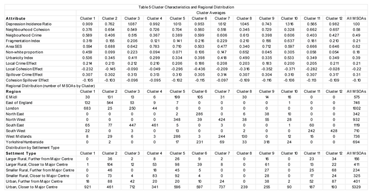
These patterns recall the notion of spatial regimes discussed above. We accordingly apply clustGeo with 12 clusters and mixing parameter 0.3, as this shows a moderate 13% loss in attribute homogeneity and a 15% loss in spatial homogeneity [48, page 1815].
Table 5 shows, for example, clusters 4 and 12 to be mostly in southern England (South East and South West), to show a low level of urbanicity, and the local crime effect (enhancing depression risk) to outweigh the local cohesion effect. By contrast, clusters concentrated in the North and Midlands, such as clusters 6, 9 and cluster 10, show the protective cohesion effect outweighing the adverse crime effect. Cluster 6, concentrated in two regions of north east England (the North East region, Yorkshire and Humberside), shows the strongest protective effect of neighborhood cohesion.
4. Discussion
There is extensive literature on the canonical disease mapping approach for disease counts, set out first by Besag et al [24], and discussed in later reviews [11,12,52]. This specifies spatially constant effects of known neighborhood risk factors, with a spatially correlated residual to represent unmodelled spatial dependencies.
The number of studies adapting this canonical approach to consider spatially varying regression coefficients or spatial volatility is, by contrast, relatively small, certainly much fewer than the number of frequentist studies applying GWR and linear model spatial volatility – for reviews of the latter see Comber et al [53] and Otto et al [29].
The lack of consideration of spatial heterogeneity in neighborhood disease studies is noted by Sridharan et al [20] using a non-Bayesian form of spatial model. This neglect of possible non-stationarity may lead to a potentially oversimplified view of risk factor effects and rules out the potential for identifying spatial regimes.
Similarly, the great majority of disease mapping studies do not evaluate the extent of spillover in environmental risk factors, where environmental risks (crime, pollution, food access, neighborhood social cohesion, etc.) are not defined by the arbitrary administrative boundaries most commonly used in disease mapping. However, acknowledging spillover is central to causal approaches to assessing neighborhood exposures. Spatial interactions are a form of network and relevant causal approaches acknowledging spillover (known as interference in the causal literature) are set out by Forastiere et al [54]. From a substantive viewpoint, the notion of extended neighborhoods, suggested by Graif [17] in relation to spillover effects in neighborhood crime, is also relevant to environmental impacts on disease.
Without considering these two respects, non-stationarity and spillover, the canonical disease model can be considered as potentially simplistic and may underestimate environmental impacts. This is certainly the case in the present study of neighborhood depression incidence, where we assess impacts of contextual neighborhood environments.
We have focused especially on contextual impacts on depression, similarly to the approach in [8], who criticize the over-emphasis on the deprivation-health link. Our findings reinforce existing evidence [7,55,56] on impacts of cohesion and crime on depression, with the spatial regime findings showing the interplay of these influences: typically, one is weaker while the other is stronger.
In terms of modelling effectiveness, we find a considerably improved fit through acknowledging non-stationarity and spillover in environmental impacts. In particular, we have shown considerable variability in impacts of social environments, especially neighborhood cohesion. Spillover effects are also considerable, especially for neighborhood crime.
5. Conclusions
We have focused in this study on contextual effects in spatial epidemiology, namely the impacts of socio-behavioral environments on neighborhood mental health. In particular, we have considered variations in neighborhood depression incidence according to levels of cohesion and crime, and aimed to provide a nuanced assessment of how these impacts operate spatially, moving beyond the simplifying assumptions of the standard Bayesian disease mapping approach. We have shown much improved fit through acknowledging non-stationarity and spillover, apparent especially in variable impacts of neighborhood cohesion, and spillover effects for neighborhood crime.
Author Contributions
PC and E A-F contributed to the script. PC was responsible for data curation, and results for models M1-M3. E A-F contributed results for model M4. All authors have read and agreed to the published version of the manuscript.
Funding
This research received no external funding
Data Availability Statement
Data and code are provided at Harvard Dataverse.
Conflicts of Interest
The authors declare no conflicts of interest.
Appendix 1. Data Sources for Predictor Variables
Data for predictors are drawn primarily from the 2021 UK Census but with some non-Census data. The index of urbanicity is based on a principal component analysis of five indicators: population density (in relation to total MSOA land area); population residential density (in relation to MOSA residential land area); distance to a primary care practice; proportions of open land; and greenspace access, specifically the proportion of greenspace within a 900 metre buffer from people’s homes. These indicators are based on the 2021 Census; on the Access to Healthy Assets and Hazards dataset (https://www.cdrc.ac.uk/); and England Land Use 2022 statistics (https://www.gov.uk/government/statistics/land-use-in-england-2022/land-use-statistics-england-2022).
Neighborhood socio-economic status (SES) is obtained from principal component analysis of three 2021 Census indicators: proportions of economically active professional and managerial; proportions of households not deprived on any dimension (Census Table TS011, Households by Deprivation Dimensions); and the unemployment rate.
Social fragmentation is obtained from principal component score of four 2021 Census indicators: residential turnover in the year 2020-2021; one person households; renting from private sector landlords (“private renting”); and non-partnered adults (not married or in civil partnership).
The crime index is from the 2019 Index of Multiple Deprivation (IMD) (https://opendatacommunities.org/data/societal-wellbeing/imd2019/indices) and measures the risk of personal and material victimization based on indicators recorded violent crimes, burglaries, thefts, and criminal damage.
Appendix 2. Cross-Scale Modelling Specification
The observed data for cross-scale modelling consist of total positive responses and total survey respondents {,for higher level spatial units, which are M=296 English local authorities. The cross-scale model framework involves regression to predict positive response rates for N=6856 lower level spatial units, followed by cumulation over these units to predict local authority rates. As mentioned in the text, the lower level units are Middle Level Super Output Areas (MSOAs). Let denote the local authority to which MSOA i=1,…,N belongs, and let denote the share of MSOA i in the population of local authority j (with these shares summing to 1 within each local authority).
Then assume a binomial likelihood at region level, ~ Bin(), where is the local authority probability of a positive outcome (belonging, trusting, chatting). The lower scale regression model for MSOAs involves predictors, a spatial random effect at MSOA level, here a conditional autoregressive model [26], and a local authority level iid random error u. This model predicts MSOA level event rates , with the region random effects ensuring that local authority event totals are closely reproduced.
The MSOA model, with a logit link, is then
logit(ri)=α+Xiβ+si+u(Ji),
and predicted region level probabilities are obtained by summing over the within the relevant local authority, namely with , weighted according to their population shares within that local authority.
Appendix 3. Non-Stationary Variance Specification: The Flexible Besag
The study [26] adapts the model of Besag et al [27] to provide the flexible Besag (fbesag) approach. The study [26] assumes subregion-specific smoothness for a single latent effect, namely the spatially varying intercept. Here we extend that framework to spatially varying regression coefficients.
The stationary model of [27] assumes a single precision . The flexible Besag instead assumes each subregion k has its own smoothness: larger produce stronger smoothing; smaller represent more local variability. We parameterize = exp(), and place fbesag priors on deviations of spatially varying coefficients around the overall fixed effect, producing nonstationary SVC surfaces. When all are equal, the model reduces to the stationary model.
Consider for simplicity, the case of a single spatially varying coefficient for predictor , without a spatially varying intercept. Then consider a negative binomial outcome ∼NB(, with a dispersion parameter, and with denoting expected cases, and denoting relative risks in neighborhood . Further let denote neighborhood spatial precisions, denote the regions to which neighborhoods i belong to, and in the equations below let , and = for neighborhoods adjacent to neighborhood . Also let be the number of neighborhoods adjacent to neighborhood in region , and .
Then the relative risk model under the fbesag prior is
where is a fixed effect coefficient, the are spatially correlated random effects constrained to sum to zero, and the conditional prior for the is
where neighborhood precisions are defined as
This specification reduces to the Besag et al model [27] when all sub-region precisions are equal.
In model M4 of Table 2, we in fact assume four spatially varying coefficients to which the fbesag prior is applied. We also keep an fbesag prior for a spatially varying intercept. We partition the MSOAs into K groups, namely the K=9 England standard regions, but other partitions are possible.
To discourage overfitting and ensure contraction to the stationary Besag [27] as a base model, we follow the penalizing complexity (PC) prior framework of Simpson et al. [28]. For a Gaussian latent component with standard deviation σ, the PC prior places an exponential penalty on σ,
which induces the precision-scale form

with calibration Pr(σ > u) = α, giving
λ = -log(α) / u, u > 0.
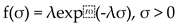
Let = (log , …, log ), with mean = (1/K) and = (I - (1/K)1), where is the flexibility parameter of s, I is an identity matrix of dimension K, and 1 is a vector of ones. Then, the joint PC prior of is stated as
f() ∝ exp(-0.5( - 1 ( - 1 ) - 0.5 - λexp(-0.5).
The λ and can be selected by the user based on some prior knowledge. The small enforces near-stationarity (k ≈ 0), while larger values allow substantively meaningful regional heterogeneity; see [26] for a detailed discussion of suitable values.
References
- Propper, C., Jones, K., Bolster, A., Burgess, S., Johnston, R., Sarker, R. (2005) Local neighborhood and mental health: evidence from the UK. Social Science and Medicine, 61(10), 2065-2083. [CrossRef]
- Lee, D. (2024) Computationally efficient localised spatial smoothing of disease rates using anisotropic basis functions and penalised regression fitting. Spatial Statistics, 59, 100796. [CrossRef]
- Mair, C., Diez Roux, A, Galea, S. (2008). Are neighborhood characteristics associated with depressive symptoms? A review of evidence. Journal of Epidemiology and Community Health, 62(11), 940-946. [CrossRef]
- March, D., Hatch, S., Morgan, C., Kirkbride, J, Bresnahan, M., Fearon, P., Susser, E. (2008) Psychosis and place. Epidemiologic Reviews, 30(1), 84-100. [CrossRef]
- Richardson, L., Hameed, Y., Perez, J., Jones, P, Kirkbride, J (2018) Association of environment with the risk of developing psychotic disorders in rural populations: findings from the social epidemiology of psychoses in East Anglia study. JAMA Psychiatry, 75(1), 75-83.
- Barnett, A., Zhang, C. J., Johnston, J, Cerin, E. (2018) Relationships between the neighborhood environment and depression in older adults: a systematic review and meta-analysis. International Psychogeriatrics, 30(8), 1153-1176. [CrossRef]
- Breedvelt, J, Tiemeier, H., Sharples, E., Galea, S., Niedzwiedz, C., Elliott, I., Bockting, C (2022). The effects of neighbourhood social cohesion on preventing depression and anxiety among adolescents and young adults: rapid review. BJPsych Open, 8(4), e97. [CrossRef]
- Wilson-Genderson, M., Pruchno, R. (2013) Effects of neighborhood violence and perceptions of neighborhood safety on depressive symptoms of older adults. Social Science and Medicine, 85, 43-49. [CrossRef]
- Pignon, B., Schürhoff, F., Baudin, G., Ferchiou, A., Richard, J, Saba, G., Szöke, A. (2016) Spatial distribution of psychotic disorders in an urban area of France: an ecological study. Scientific Reports, 6(1), 26. [CrossRef]
- Cruz, J., Li, G., Aragon, M, Coventry, P, Jacobs, R., Prady, S, White, P (2022). Association of environmental and socioeconomic indicators with serious mental illness diagnoses identified from general practitioner practice data in England: A spatial Bayesian modelling study. PLoS medicine, 19(6), e1004043. [CrossRef]
- Kirkbride, J, Lunn, D, Morgan, C., Lappin, J, Dazzan, P., Morgan, K., Jones, P (2010). Examining evidence for neighborhood variation in the duration of untreated psychosis. Health and Place, 16(2), 219-225. [CrossRef]
- Lawson, A, Lee, D (2017) Bayesian Disease Mapping for Public Health. Chapter 16 in Handbook of Statistics, Science Direct. [CrossRef]
- Waller L, Carlin B (2010) Disease mapping. Chapter 14 In Handbook of Modern Statistical Methods, Chapman Hall CRC, pp 217–243.
- Reich, B, Yang, S., Guan, Y., Giffin, A, Miller, M, Rappold, A. (2021). A review of spatial causal inference methods for environmental and epidemiological applications. International Statistical Review, 89(3), 605-634. [CrossRef]
- Anselin, L. (2002) Under the hood issues in the specification and interpretation of spatial regression models. Agricultural Economics, 27(3), 247-267.
- Giffin, A., Reich, B, Yang, S., Rappold, A (2023) Generalized propensity score approach to causal inference with spatial interference. Biometrics, 79(3), 2220-2231. [CrossRef]
- Sarrias, M., Molina-Varas, A. (2022). Your air pollution makes me sick!: Estimating the spatial spillover effects of PM2. 5 emissions on emergency room visits in Chile. Region, 9(2), 1-23. [CrossRef]
- Graif, C. (2015). Delinquency and gender moderation in the moving to opportunity intervention: The role of extended neighborhoods. Criminology, 53(3), 366-398. [CrossRef]
- 19. Fotheringham, A, Brunsdon, C, Charlton M (2002) Geographically Weighted Regression: The Analysis of Spatially Varying Relationships, Wiley: New York.
- Vidoli F, Benedetti R (2022) SpatialRegimes package: a brief introduction to spatial clusterwise regression with a focus on SkaterF function. https://fvidoli.shinyapps.io/SpatialRegimes_app/.
- Sridharan, S., Koschinsky, J, Walker, J (2011). Does context matter for the relationship between deprivation and all-cause mortality? The West vs. the rest of Scotland. International Journal of Health Geographics, 10(1), 33. [CrossRef]
- Giordano, V., Rigatti, T., Shaikh, A., Ferraioli, T. (2023). Spatial health predictors for depressive disorder in Manhattan: a 2020 analysis. Cureus, 15(7). [CrossRef]
- Choi, H., Kim, H. (2017). Analysis of the relationship between community characteristics and depression using geographically weighted regression. Epidemiology and Health, 39, e2017025. [CrossRef]
- Leyk, S., Norlund, P, Nuckols, J (2012) Robust assessment of spatial non-stationarity in model associations related to pediatric mortality due to diarrheal disease in Brazil. Spatial and Spatio-temporal Epidemiology, 3(2), 95-105. [CrossRef]
- Assunção, R (2003) Space varying coefficient models for small area data. Environmetrics, 14(5), 453-473. [CrossRef]
- Fattah E, Krainski E, van Niekerk J, Rue H (2024) Non-stationary Bayesian spatial model for disease mapping based on sub-regions. Statistical Methods in Medical Research, 33(6): 1093-1111.
- Besag, J., York, J., Mollié, A. (1991) Bayesian image restoration, with two applications in spatial statistics. Annals of the Institute of Statistical Mathematics, 43, 1-20. [CrossRef]
- Simpson D, Rue H, Riebler A, Martins T, Sørbye, S (2017) Penalising model component complexity: a principled, practical approach to constructing priors. Statist. Sci. 32 (1) 1 – 28. [CrossRef]
- Yan, J. (2007) Spatial stochastic volatility for lattice data. Journal of Agricultural, Biological, and Environmental Statistics, 12(1), 25–40. [CrossRef]
- Otto, P., Doğan, O., Taşpınar, S., Schmid, W, Bera, A (2025) Spatial and spatiotemporal volatility models: A review. Journal of Economic Surveys, 39(3), 1037-1091. [CrossRef]
- Arambepola, R., Lucas, T, Nandi, A, Gething, P, Cameron, E (2022) A simulation study of disaggregation regression for spatial disease mapping. Statistics in Medicine, 41(1), 1-16. [CrossRef]
- Sturrock H, Cohen J, Keil P, Tatem A, Le Menach A, Ntshalintshali N, Hsiang M, Gosling R (2014) Fine-scale malaria risk mapping from routine aggregated case data. Malaria Journal, 13(1), 421. [CrossRef]
- Shaw, E, Sutcliffe, D., Lacey, T., Stokes, T. (2013) Assessing depression severity using the UK Quality and Outcomes Framework depression indicators: a systematic review. Br J General Practice, 63(610), e309. [CrossRef]
- Forbes L, Marchand C, Doran T, Peckham S (2017) The role of the Quality and Outcomes Framework in the care of long-term conditions: A systematic review. Br J General Practice, 67(664): e775-e784. [CrossRef]
- Kirkbride, J, Anglin, D, Colman, I., Dykxhoorn, J., Jones, P, Patalay, P, Griffiths, S (2024) The social determinants of mental health and disorder: evidence, prevention and recommendations. World Psychiatry, 23(1), 58-90. [CrossRef]
- Tsimpida, D., Tsakiridi, A., Daras, K., Corcoran, R., Gabbay, M (2024) Unravelling the dynamics of mental health inequalities in England: a 12-year nationwide longitudinal spatial analysis of recorded depression prevalence. SSM-Population Health, 26, 101669. [CrossRef]
- Allardyce, J, Gilmour, H, Atkinson, J, Rapson, T, Bishop, J, McCreadie, R (2005) Social fragmentation, deprivation and urbanicity: relation to first-admission rates for psychoses. Brit J. Psych, 187(5), 401-406. [CrossRef]
- Curtis, S., Congdon, P, Atkinson, S., Corcoran, R., MaGuire, R., Peasgood, T. (2019) Individual and local area factors associated with self-reported wellbeing, perceived social cohesion and sense of attachment to one’s community: analysis of the Understanding Society Survey: Research Report. What Works for Wellbeing Technical Report. Durham Research Online, http://dro.dur.ac.uk.
- Buckner, J (1988) The development of an instrument to measure neighborhood cohesion. Amer J Comm Psych, 16(6), 771-791. [CrossRef]
- Choi, Y, Ailshire, J (2024). Perceived neighborhood disorder, social cohesion, and depressive symptoms in spousal caregivers. Aging and Mental Health, 28(1), 54-61. [CrossRef]
- Chan, J., To, H, Chan, E. (2006). Reconsidering social cohesion: Developing a definition and analytical framework for empirical research. Social Indicators Research, 75(2), 273-302. [CrossRef]
- Sampson, L., Ettman, C, Galea, S. (2020) Urbanization, urbanicity, and depression: a review of the recent global literature. Current Opinion in Psychiatry, 33(3), 233-244. [CrossRef]
- Dempsey, N., Brown, C., Raman, S., Porta, S., Jenks, M., Jones, C., Bramley, G. (2010) Elements of urban form. Chapter 2 in Dimensions of the Sustainable City, M. Jenks and C. Jones (eds), Springer pp 21-51.
- Baranyi, G., Cherrie, M., Curtis, S., Dibben, C., Pearce, J (2020) Neighborhood crime and psychotropic medications: a longitudinal data linkage study of 130,000 Scottish adults. American Journal of Preventive Medicine, 58(5), 638-64. [CrossRef]
- Williams, E. D., Tillin, T., Richards, M., Tuson, C., Chaturvedi, N., Hughes, A, Stewart, R. (2015) Depressive symptoms are doubled in older British South Asian and Black Caribbean people compared with Europeans: associations with excess co-morbidity and socioeconomic disadvantage. Psychological Medicine, 45(9), 1861-1871. [CrossRef]
- Department for Culture, Media & Sport (2024) Community Life Survey 2023/24 Online Questionnaire. https://assets.publishing.service.gov.uk.
- Lunn, D., Spiegelhalter, D., Thomas, A, Best, N. (2009) The BUGS project: Evolution, critique and future directions. Statistics in Medicine, 28(25), 3049-3067. [CrossRef]
- Department for Culture, Media & Sport (2024) Community Life Survey 2023/24: Neighbourhood and community. https://www.gov.uk/government/statistics/community-life-survey-202324-annual-publication/community-life-survey-202324-neighbourhood-and-community.
- Chavent M, Kuentz-Simonet V, Labenne A, Saracco J (2018) ClustGeo: an R package for hierarchical clustering with spatial constraints. Comput Stat , 33: 1799-1822. [CrossRef]
- Spiegelhalter, D, Best, N, Carlin, B, van der Linde, A (2002) Bayesian measures of model complexity and fit. Journal of the Royal Statistical Society, Series B. 64 (4): 583–639. [CrossRef]
- Watanabe, S (2013) A Widely Applicable Bayesian Information Criterion. Journal of Machine Learning Research. 14: 867–897.
- Office of National Statistics (2025) 2021 Rural Urban Classification. https://www.ons.gov.uk/methodology/geography/geographicalproducts/ruralurbanclassifications/2021ruralurbanclassification.
- Kang, S., Cramb, S., White, N., Ball, S., Mengersen, K. (2016) Making the most of spatial information in health: a tutorial in Bayesian disease mapping for areal data. Geospatial health, 11(2). [CrossRef]
- Comber, A., Brunsdon, C., Charlton, M., Dong, G., Harris, R., Lu, B, Harris, P. (2023). A route map for successful applications of geographically weighted regression. Geographical Analysis, 55(1), 155-178. [CrossRef]
- Forastiere L, Airoldi E, Mealli F (2021) Identification and estimation of treatment and interference effects in observational studies on networks, J. Amer. Stat. Assoc., 116, 901–918. [CrossRef]
- Mair, C., Roux, A, Shen, M., Shea, S., Seeman, T., Echeverria, S, O'meara, E (2009). Cross-sectional and longitudinal associations of neighborhood cohesion and stressors with depressive symptoms in the multiethnic study of atherosclerosis. Annals of epidemiology, 19(1), 49-57. [CrossRef]
- Bassett, E., Moore, S. (2013). Social capital and depressive symptoms: the association of psychosocial and network dimensions of social capital with depressive symptoms in Montreal, Canada. Social Science & Medicine, 86, 96-102. [CrossRef]
Figure 1.
Varying Local Cohesion Regression Effect.
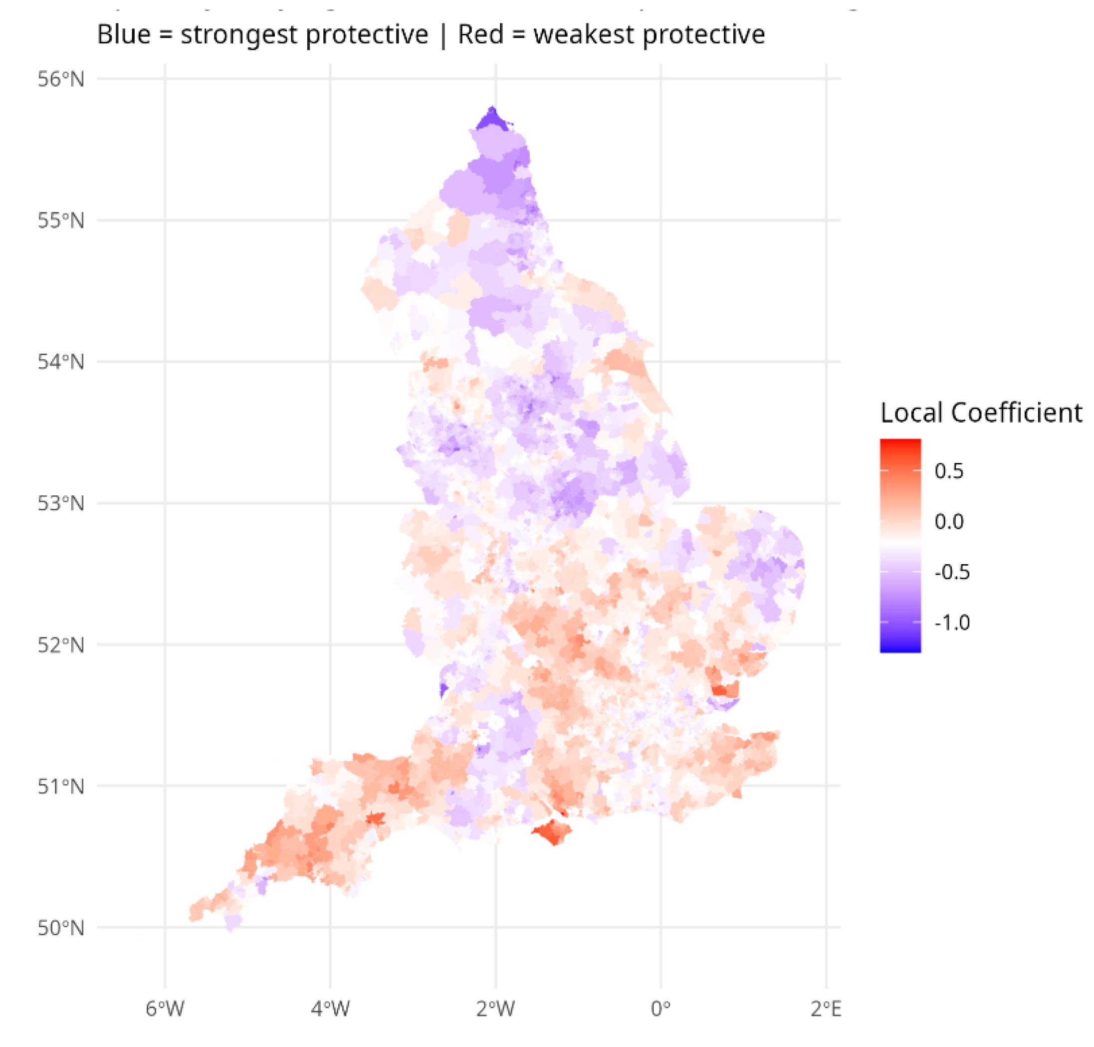
Figure 2.
Varying Local Crime Regression Effect.
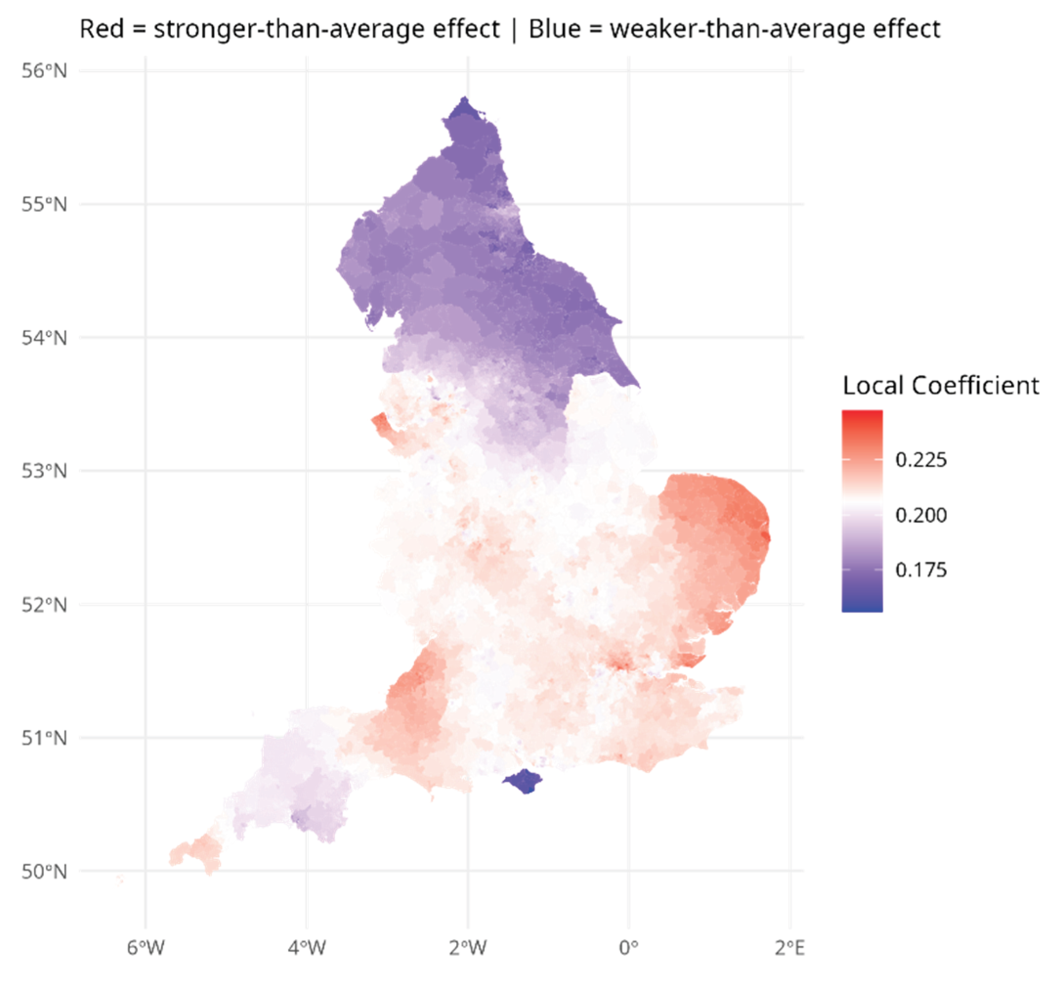

Table 1.
Cross-Scale Neighborhood Regression Results.
| Log Odds Ratio Coefficients | |||
| Sense of Belonging | |||
| Mean | 2.5% | 97.5% | |
| Area SES | 0.49 | 0.21 | 0.73 |
| Proportion Non-white | -0.22 | -0.40 | 0.02 |
| Urbanicity | -1.35 | -1.73 | -0.99 |
| Many Neighbors can be Trusted | |||
| Mean | 2.5% | 97.5% | |
| Area SES | 2.78 | 2.56 | 3.07 |
| Proportion Non-white | -0.85 | -1.14 | -0.63 |
| Urbanicity | -1.90 | -2.29 | -1.40 |
| Chat with Neighbors More than Once a Month | |||
| Mean | 2.5% | 97.5% | |
| Area SES | -0.12 | -0.38 | -0.12 |
| Proportion Non-white | -0.34 | -0.51 | -0.34 |
| Urbanicity | -2.74 | -3.05 | -2.75 |
Table 2.
Percentages of Neighborhoods (MSOAs) with High Cohesion by Region and Urban Level.
| Settlement Category | ||||
| Region | Larger rural | Smaller rural | Urban | Total |
| East Midlands | 47 | 76 | 9 | 22 |
| Eastern England | 34 | 66 | 11 | 22 |
| London | - | - | 3 | 3 |
| North East | 24 | 100 | 11 | 15 |
| North West | 66 | 95 | 15 | 21 |
| South East | 55 | 91 | 15 | 25 |
| South West | 54 | 99 | 12 | 33 |
| West Midlands | 63 | 98 | 9 | 19 |
| Yorkshire-Humber | 64 | 100 | 11 | 21 |
| All of England | 50 | 88 | 10 | 20 |
Table 3.
Predicting Neighbourhood Depression Incidence.
| Coefficients represent Logged Relative Risks with Predictors on [0,1] scale | ||||
| Model Specification (and Identifier) | Parameter Profile | |||
| Baseline (M1) | Mean | St devn | 2.5% | 97.5% |
| Intercept | 0.039 | 0.045 | -0.050 | 0.127 |
| Area SES | -0.149 | 0.042 | -0.231 | -0.066 |
| Proportion Non-white | 0.031 | 0.038 | -0.043 | 0.106 |
| Crime Index | 0.285 | 0.040 | 0.207 | 0.363 |
| Neighbourhood Cohesion | -0.276 | 0.053 | -0.379 | -0.173 |
| Including Spatial Lags (Cohesion, Crime) (M2) | Mean | St devn | 2.5% | 97.5% |
| Intercept | 0.012 | 0.095 | -0.174 | 0.198 |
| Area SES | -0.192 | 0.043 | -0.276 | -0.108 |
| Proportion Non-white | -0.013 | 0.039 | -0.089 | 0.064 |
| Crime Index | 0.243 | 0.040 | 0.165 | 0.322 |
| Neighbourhood Cohesion | -0.191 | 0.054 | -0.297 | -0.086 |
| Crime Spillover | 0.306 | 0.085 | 0.139 | 0.473 |
| Cohesion Spillover | -0.195 | 0.082 | -0.356 | -0.035 |
| Non-Stationary Environments (Cohesion, Crime) and Spatial Lags (M3) | Mean | St devn | 2.5% | 97.5% |
| Intercept | 0.028 | 0.094 | -0.156 | 0.211 |
| Area SES | -0.150 | 0.042 | -0.231 | -0.068 |
| Proportion Non-white | -0.044 | 0.038 | -0.118 | 0.031 |
| Crime Index | 0.242 | 0.040 | 0.163 | 0.321 |
| Neighbourhood Cohesion | -0.274 | 0.053 | -0.378 | -0.169 |
| Crime Spillover | 0.300 | 0.084 | 0.135 | 0.465 |
| Cohesion Spillover | -0.178 | 0.079 | -0.334 | -0.022 |
| Non-Stationary Environments, Spatial Lags and Non-Stationary Region Precisions (M4) | Mean | St devn | 2.5% | 97.5% |
| Intercept | 0.034 | 0.095 | -0.152 | 0.220 |
| Area SES | -0.249 | 0.041 | -0.329 | -0.169 |
| Proportion Non-white | -0.089 | 0.038 | -0.162 | -0.015 |
| Crime Index | 0.206 | 0.040 | 0.128 | 0.284 |
| Neighbourhood Cohesion | -0.219 | 0.052 | -0.321 | -0.118 |
| Crime Spillover | 0.309 | 0.085 | 0.143 | 0.475 |
| Cohesion Spillover | -0.104 | 0.079 | -0.259 | 0.051 |
| Model Fit | ||||
| M1 | M2 | M3 | M4 | |
| DIC | 58647 | 58519 | 58010 | 56307 |
| WAIC | 58173 | 58098 | 57431 | 55359 |
| Mean Absolute Deviation | 4.916 | 4.882 | 4.415 | 3.334 |
Table 4.
Regional Patterns of Risk and Risk Factor Impacts: Standard Regions and Settlement Types.
| Fitted Relative Risks of Depression Incidence | ||||
| Region | Larger rural | Smaller rural | Urban | All Settlement Types |
| East Midlands | 0.79 | 0.77 | 0.84 | 0.82 |
| East of England | 0.75 | 0.64 | 0.76 | 0.74 |
| London | - | - | 0.93 | 0.93 |
| North East | 0.95 | 0.72 | 1.10 | 1.07 |
| North West | 1.12 | 1.08 | 1.50 | 1.46 |
| South East | 0.99 | 1.00 | 1.06 | 1.05 |
| South West | 0.76 | 0.76 | 0.87 | 0.84 |
| West Midlands | 1.04 | 0.93 | 1.17 | 1.15 |
| Yorks/Humberside | 0.74 | 0.66 | 0.90 | 0.87 |
| England | 0.86 | 0.82 | 1.03 | 1.00 |
| Environmental Risk Factor Impacts | ||||
| Larger rural | Smaller rural | |||
| ` | Crime Effect | Cohesion Effect | Crime Effect | Cohesion Effect |
| East Midlands | 0.20 | -0.26 | 0.20 | -0.26 |
| East of England | 0.22 | -0.12 | 0.22 | -0.20 |
| London | - | - | - | - |
| North East | 0.17 | -0.40 | 0.17 | -0.48 |
| North West | 0.19 | -0.26 | 0.19 | -0.24 |
| South East | 0.21 | -0.04 | 0.21 | -0.04 |
| South West | 0.21 | -0.10 | 0.21 | -0.10 |
| West Midlands | 0.21 | -0.15 | 0.21 | -0.16 |
| Yorks/Humberside | 0.19 | -0.35 | 0.18 | -0.31 |
| England | 0.20 | -0.19 | 0.21 | -0.16 |
| Urban | All Settlement Types | |||
| Region | Crime Effect | Cohesion Effect | Crime Effect | Cohesion Effect |
| East Midlands | 0.20 | -0.30 | 0.20 | -0.29 |
| East of England | 0.21 | -0.16 | 0.22 | -0.16 |
| London | 0.21 | -0.23 | 0.21 | -0.23 |
| North East | 0.18 | -0.41 | 0.18 | -0.41 |
| North West | 0.21 | -0.32 | 0.20 | -0.31 |
| South East | 0.21 | -0.06 | 0.21 | -0.05 |
| South West | 0.21 | -0.17 | 0.21 | -0.15 |
| West Midlands | 0.21 | -0.17 | 0.21 | -0.17 |
| Yorks/Humberside | 0.19 | -0.39 | 0.19 | -0.38 |
| England | 0.21 | -0.23 | 0.21 | -0.22 |
Disclaimer/Publisher’s Note: The statements, opinions and data contained in all publications are solely those of the individual author(s) and contributor(s) and not of MDPI and/or the editor(s). MDPI and/or the editor(s) disclaim responsibility for any injury to people or property resulting from any ideas, methods, instructions or products referred to in the content. |
© 2025 by the authors. Licensee MDPI, Basel, Switzerland. This article is an open access article distributed under the terms and conditions of the Creative Commons Attribution (CC BY) license (http://creativecommons.org/licenses/by/4.0/).
Copyright: This open access article is published under a Creative Commons CC BY 4.0 license, which permit the free download, distribution, and reuse, provided that the author and preprint are cited in any reuse.


