
Submitted:
28 November 2025
Posted:
28 November 2025
You are already at the latest version
Abstract
Flooding episodes caused by a heavy rainfall event has become more frequent especially during the rainfall season in Botswana, this poses some socio-economic and environmental risks. This study investigates the capability of Weather Research and Forecasting (WRF) in simulating a heavy rainfall event which occurred on the 26th of December 2023 in Mahalapye District, Botswana. This event is one amongst many which has had negatively impacted the lives and infrastructures in Botswana. The WRF model was configured using the tropical-suite physics schemes, i.e. (Rapid Radiative Transfer Model, Yonsei University planetary boundary layer scheme, Unified Noah land surface model, New Tiedtke, Weather Research and Forecasting Single-Moment 6-class) on a two-way nested domain (9 km and 3 km grid-spacing) and was initialized with GFS dataset. Gauged station data was used for validation alongside synoptic charts from GFS and ECMWF ERA5 dataset. The results show that the WRF model simulation using the Tropical-Suite physics Schemes is able to reproduce the spatial and temporal patterns of the observed rainfall but with some notable biases. Performance metrics including RMSE, correlation coefficient and KGE showed moderate to good agreement highlighting the model’s sensitivity to physical parameterization and resolution. The results of this study concludes that the WRF model demonstrates promising potential in forecasting extreme rainfall events in Botswana but more sensitivity tests to different parameterization schemes are needed in order to integrate the model into the early warning systems to enhance disaster preparedness and response.
Keywords:
WRF model
; tropical-suite physics schemes
; extreme rainfall
; Mahalapye District
; model validation
1. Introduction
Global concerns over extreme events are highlighted by [1], Indicating that several extreme climate events are increasing in frequency and intensity due to anthropogenic climate change, hence raising the likelihood of impacts associated with urbanization. [2] also stated that climate change could cause increased frequency in droughts and floods. [1,2] observed that climate change may cause climate variability, changes in average precipitation and extreme events occurrences. [3] provided an analysis of flood occurrences and their impacts over a five-year period (2015-2019). The report indicated that flood episodes have increased in Botswana and are caused by heavy rainfall, inadequate drainage systems and growth of settlements into locations susceptible to flooding. [3] showed that the most affected areas in Botswana were Ghanzi, Northeast, Central, Kweneng, Kgatleng, and Southern Districts, where infrastructure and human settlements have been significantly impacted. The findings from [3] indicated an increase in occurrence and severity of floods in Botswana with a recommendation that integrating meteorological forecasting, hydrological modeling and community-based disaster preparedness will be essential in mitigating the socio-economic impacts of future flood event. With increased occurrences of extreme events, especially floods their impacts leave an everlasting effect on the affected communities. With the recurring floods, there are significant impacts to both socio-economic and environmental impacts. The study by [4] highlighted that the 2016/2017 floods caused damage to property and infrastructure, livestock losses, crop damage and human health impacts. The authors estimated that the financial cost to the damage was around BWP 2,407,436 and this amount excludes crop losses since there were no monetary estimates done from the study. [5] did a study on the floods which affected the Okavango Delta communities in 2004 and 2009. The researchers found that the floods caused crop losses in Tubu and Shorobe Villages of 67% and 72%, respectively. [6] conducted an assessment of rainfall variability and vulnerability to floods and droughts. The study highlights that Mahalapye’s flood vulnerability is increased by the presence of two rivers (Mahalapye River and Rakabeswa River) which pass through the town and settlement areas of Mahalapye.
Botswana has established several disaster management frameworks: The National Disaster Risk Management Plan (NDRMP) of 2009, this plan outlines the structure for response, preparedness and recovery, National Disaster Risk Reduction Strategy (NDRRS) 2013 - 2018 intended to reduce disaster vulnerability and promote resilience and National Policy on Disaster Management (NPDM) of 1996. The policy aims to coordinate disaster response efforts. [7], in their article, found that National Disaster Risk Reduction Strategy (NDRRS) lacks community involvement, detailed guidance on emergency procedures and initiative-taking risk mitigation measures. The NDRMP has been shown to be overly sector-focused, lacking provisions for community-level response and localized disaster prevention [7]. The authors further states that the NPDM is outdated, limited to a relief-focused approach and lacks mechanisms for systematic updates or community engagement and they conclude by outlining that a major finding relevant to the study was lack of geospatial technology integration and real-time data systems in disaster planning, this affects the early warning capabilities and as a result affects real-time response efficiency. The findings suggest that it is time the country incorporates dynamical modelling in an attempt to detect extreme rainfall events using Regional Climate Models (RCMs’) also known as Limited Area Models (LAMs’) in Numerical Weather Prediction (NWP).
Intense precipitation accompanied by strong winds often highlight the presence of severe weather systems. A significant component of what makes weather patterns develop is the continuous transfer of energy, moisture and momentum between the terrestrial surface and the atmosphere. Meteorologists aim to figure out how these relationships work because they are key to understanding why heavy rain take place [8,9]. Global Circulation Models (GCMs’) are used to make weather forecasts over a range of time periods [10,11]. GCMs’ are not able to capture the mesoscale processes which contribute to rainfall. They do not show important mesoscale and local sub-grid features like convective processes (updrafts and downdrafts associated with thunderstorms and other convective systems) and they tend to overestimate rainfall [11,12]. To improve the representation of regional and local weather-related phenomena, LAMs’ were developed as a dynamical down-scaling approach [13,14]. Unlike GCMs’, LAMs’ operate at higher grid spacing (1 – 50 km), allowing for better simulation of orographic precipitation, convective processes and land-sea interactions [15,16].
LAMs’ serve as a supplementary research approach, facilitating further process investigations and the simulation of regional and local situations using the downscaling technique [17]. Downscaling technique using LAMs’, magnifies the outputs of GCMs’. LAM can generate improved regional meteorological data that aligns with the large-scale circulation from global reanalysis data or general circulation models (GCMs), utilizing precise representations of physical processes and high grid-spacing to capture complex topography, land-sea contrasts and land use. [18]. Researchers including [19] have been developing a LAM called WRF model -an advanced NWP system designed for both operational forecasting and atmospheric research. WRF is an open-source community model used for research and numerical weather prediction [19] as well as a medium range forecasting. The WRF model was developed by the National Center for Atmospheric Research (NCAR); however, the Mesoscale and Microscale Meteorology (MMM) division of the University Cooperation for Atmospheric Research (UCAR) continues to maintain and update the WRF model [11,20]. In the late 1990s’, WRF developers began to produce a research-operations system for next-generation NWP capacity. The WRF model is a completely compressible, non-hydrostatic mesoscale NWP model with topography following sigma coordinates [11,20]. [21] applied WRF model at a high grid-spacing of 2.5 km to study weather extreme events and integrate the model into Extreme Rainfall Detection System (ERDS). The authors found out that it can improve early detection and warning of extreme rainfall events especially by assimilating observations into the WRF model.
Between the 16th and 23rd of January 2013, a total of 4210 people (at least 842 families) suffered as their households were destroyed by the widespread thunderstorms which caused extensive flooding in the Central District of Botswana, also affecting the Mahalapye District [22]. The floods displaced many residents and resulted in majority of them living in tents even weeks later while their houses were being rebuild. This episode highlighted among others the absence of a reliable early warning and prediction system. A solution to this problem might be NWP specifically dynamic modeling. The low grid-spacing of most GCMs’ is unsuitable for heavy rainfall analysis thus, LAMs’ can be utilized to estimate rainfall at small grid spacing [23]. This study aims to assess the ability of the WRF model in simulating high rainfall event within the Mahalapye District of Botswana highlighting the limitation and areas of improvement on the WRF model and it adopts the WRF tropical suite physics schemes configuration which is recommended for the tropical belt and subtropical regions [24]. This suite has been tested and consistently demonstrates good performance under tropical thermodynamic conditions. [25] used the tropical suite as a baseline and later applied sensitivity tests and it showed that variations in microphysics (WSM6 vs Thompson) and PBL formulations (YSU, MYJ, ACM2) exerted more influence on rainfall structure localization. Their results showed that the single-moment WSM6 scheme outperformed the double-moment Thompson scheme while non-local PBL formulations (YSU, ACM2) was found to produce realistic low-level mixing and delayed convective triggering compared with the local WYJ. Also [26] reported that in the Southern Africa region, WSM6 coupled with non-local PBL schemes best represented convective intensity and timing, highlighting that PBL dynamics plays a big role over rainfall structure than microphysical complexity. [27] also confirmed that RRTM-YSU-WSM6-Noah configuration (tropical suite) was able to reproduce the diurnal evolution of boundary-layer fluxes, cloud depth and storm organization which outperformed a different scheme used in mid-latitudes called CONUS suite. The choice of the tropical suite for this study follows the collective studies mentioned which all concluded that tropical suite configuration is relevant for Southern Africa region.
Most of the WRF studies especially run over Botswana are focusing on investigating the tropical cyclones which made landfall over the continent and subsequently reaching Botswana as a tropical depression. [28] study focused on tropical cyclone Dineo using WRF and in that study, it was found that the different model configurations tested to simulate the heavy rainfall received are generally similar. However, observations still remain relevant in modern day NWP. This highlights the gap and relevance of the study to apply the WRF model to simulate/predict other extreme rainfall events not restricted to tropical cyclones.
2. Materials and Methods
2.1. Study Area
Botswana is a landlocked country in southern Africa, located between latitudes 18°– 27°S and longitudes 20°– 29°E. The country spans 582,000 km2 and has a population of over 2 million [29]. Botswana has new addition in the administrative boundaries which were initially 10 in total. The districts were Ngamiland, Chobe, Gantsi, Kgalagadi, Southern, Southeast, Kgatleng, Kweneng, Central and Northeast. Botswana has divided its districts by subdividing some of the existing districts bringing the total to twenty-six (26) districts. The Central District has been divided into eight (8) more districts. The Mahalapye District is the primary focus area for this study and its geographically located in the southeastern parts of the Central District (see Figure 1 below). The Mahalapye District population is approximately 48,431 according to Statistics Botswana [30].
2.2. Source of Data
Global Forecasting System (GFS) model provides global coverage forecasts across the globe with a horizontal resolution of approximately and this is equivalent 28 km grid spacing at the equator. The data is freely available from the National Centers for Environmental Prediction (NCEP) file transfer server (FTP) https://ftp.ncep.noaa.gov/data/nccf/com/gfs/prod/. The dataset is updated daily and includes parameters such as temperature, humidity, wind speed and direction, geopotential height, surface pressure and precipitation. The data is provided in GRIB2 format and updated every six hours (00, 06, 12 and 18 UTC forecast cycle) and available at three hours intervals for forecast periods of up to 16 days ahead [31].
For this study, the WRF model used GFS datasets, from the 00 UTC cycle as initial and lateral boundary conditions. This dataset contains GFS model outputs at a global scale detailing the atmospheric state according to GFS and provides WRF model initialization from short to medium range forecasting and it can be used for extreme weather events model simulation as highlighted by [32,33]. GFS data has also been used in Botswana by [28] and also in upper Ganga Basin by [23]. BDMS has 18 synoptic stations and over 600 rainfall stations scattered across the country. The rainfall stations are placed in most of the government owned premises such as schools, police stations and some army bases to mention a few. For this study, a total of six (6) stations available in Mahalapye district were used namely, Kalamare Primary School, Mahalapye Meteorological Station, Machaneng Police, Pallaroad Kgotla, Mookane Primary School and Tirelo Primary School, see (Figure 1). Their respective latitudes, longitudes and altitude are shown in Table 1 below.
The data used was supplied by the BDMS, which maintains a quality standard and ensures that the gauged weather stations are serviced on annual basis by a team of engineers before the onset of a rainfall season. The data is readily available from BDMS and can be used for research purposes as it has been used by [34] who employed monthly precipitation data from 60 stations provided by BDMS, covering the data period from 1981 to 2016, to analyse rainfall patterns in Botswana, additionally, [35] utilised daily precipitation data from 76 rain gauge stations across Botswana to develop regional Intesity Duration Frequency (IDF) curves for ungauged sites, aiding to the estimation of design storm depths. [36] analyzed historical monthly rainfall data from the Palapye police weather station, provided by BDMS, to assess climate change and variability in the region and lastly [37] explored the influence of climate variability on rainfall characteristics in the Shashe catchment, utilizing observed data from 1981 to 2020 provided by BDMS and used a Coupled Model Intercomparison Project Phase 5 General Circulation Models to produce future projections of rainfall for 2021–2050.
To complement the gauged rainfall observations from BDMS network, large-scale atmospheric fields were derived from European Center for Medium-Range Weather Forecasts (ECMWF) ERA5 reanalysis. ERA5 dataset provides a consistent representation of the state of the global atmosphere, generated through an advanced four-dimensional variational (4D-Var) data assimilation system that also integrates satellite, surface and upper-air observations [38]. The horizontal resolution of ERA5 data is and a total of 137 hybrid sigma-pressure levels which extends from the surface to around 0.01 hPa which offers detailed diagnostics of vertical atmospheric structure. The data is also suitable for assessing the large-scale drivers and moisture transport process that influences convection development over the Southern Africa [39,40]. In addition, ERA5 dataset has shown strong agreement with in-situ and satellite observations across Africa when compared to the earlier ERA-interim dataset [41], especially key meteorological variables such as precipitation and humidity [42].
2.3. Numerical Study design
The current study uses the Advanced WRF model, version 4.4.1, released in August 2021. The WRF version 4.4.1 was an update on the WRF version 4.4. The WRF model produces output every three hours using a two-way nesting in this simulation. In a two-way nesting configuration, the lateral boundary conditions are sent from the parent domain to the child nest and the values in the child domain (higher resolution domain) are averaged to the corresponding value in the parent domain (lower resolution domain). The outer domain (parent domain), which has a horizontal resolution of 9 km, covers most of Southern Africa and parts of the Atlantic and Indian Oceans. The 9 km domain setup is nested with an inner domain (Child domain) at a horizontal resolution of 3 km centered over Botswana, covering some parts of its neighbouring countries as shown in Figure 2.
The WRF model was initialized with GFS data which has a grid-spacing of approximately 28 km (0.25°). GFS pgrb2 format is used to provide both initial boundary conditions and lateral boundary conditions with a time step of 3 hours. The model used the Runge-Kutta 3-time integration scheme, which solves equations representing atmospheric processes over small-time intervals to produce a forecast [19]. The WRF model simulation was initialised on the 24th December 2023 at 00:00 UTC with a lead time of 48 hours to simulate the extreme event. In order to account for the 48 hours of the severe rain which occurred on 26th December 2023, the model is set up to produce a forecast for a maximum of 120 hours, or five days of simulation. Table 2 shows the WRF model tropical suite configuration. The model simulation used the Tropical suite configuration since Botswana is located within the sub-tropics, and the “tropical suite” as proposed by [43] integrates several schemes which are suitable for tropical environments (see Table 3 below);
2.4. Model Evaluation Statistics
2.4.1. Root Mean Square Error
In assessing the accuracy of the WRF model simulation against observed rainfall data, bias, correlation and event probability of detection capabilities were used with a key focus on extreme rainfall. This study used a range of widely accepted statistical metrics, i.e. Root Mean Square Error (RMSE), Kling-Gupta Efficiency (KGE), Percentage Bias (% Bias), Pearson’s Correlation Coefficient (r), Probability of Detection (POD) and Variability Ratio (VR).
As demonstrated by [48], equation 1, the RMSE, shows the average magnitude of the error between the observed rainfall from BDMS gauged stations and the corresponding WRF - simulated rainfall, is one of the statistical metrics that have been used and applied in atmospheric modeling to quantify model performance and to evaluate predictive reliability. This metrics allocates more weight to bigger differences between observed (station) rainfall and simulated (WRF) rainfall because they are squared, overall, the method is effective in identifying extreme events since it imposes more penalties on large errors [49]. A lower RMSE value translate to enhanced model accuracy while a higher value indicates a lower model accuracy.
where is the model-predicted value, is the observed value, and n is the number of observations.
2.4.2. Percent Bias
Percent Bias (PBIAS) is a statistical metrics used to show how frequent a model tends to overestimate or underestimate observations and computes it as a percentage. [50] highlighted that PBIAS is an important measure for hydrological, meteorological and atmospheric modeling for identifying systematic errors in simulations. PBIAS is calculated as shown in equation 2
where = predicted value (simulated), = observed value (measured), n = number of observations.
2.4.3. Pearson’s Correlation Coefficient
Pearson’s correlation coefficient (PCC) is also a widely used statistical metrics in many modelling studies. It is mainly used for model validation because the metrics has the ability to quantify how well a model is able to reproduce observed values [51,52]. In the context of evaluating the WRF outputs, the metrics is able to measure the variation between the simulated and the observed rainfall and as a result it assesses how well the WRF model captures the temporal and spatial patterns in observed rainfall. PCC is calculated as follows; equation 3.
where r = Pearson’s correlation coefficient,
= WRF-simulated rainfall value,
= observed rainfall value (from BDMS gauges),
= mean of simulated and observed rainfall, respectively,
n = total number of observations (stations or time steps).
In this validation study, high r values imply that the model is good at capturing the timing and sequence of a rainfall event even if there are discrepancies in the absolute magnitudes.
2.4.4. Probability of Detection
According to [52], Probability of Detection (POD), equation 4, is defined as the ratio of the model being able to predict/reproduce an occurrence (hits) to the total number of observed events (hits + misses). The current study applies the POD to quantify the WRF’s effectiveness in identifying the occurrence of rainfall with a threshold of 1 mm.
where: Hits = Number of times the event was correctly predicted,
Misses = Number of times the event occurred but was not predicted.
2.4.5. Kling-Gupta Efficiency
Kling-Gupta Efficiency (KGE) is a robust performance metrics which combines three key components: correlation, bias and variability into a single diagnostic value [53]. KGE addresses some limitations of the traditional Nash-Sutcliffe Efficiency by ensuring a more balanced representation of error sources. The KGE is illustrated in equation 5.
KGE values range from to 1, with 1 indicating an agreement between the observations and the model prediction while 0 suggests that the model does not perform better than the mean observed data and negative values indicate poor performance [53].
2.4.6. Haversine formula
Many model evaluation studies often interpolate simulated model outputs to observational locations, this implies comparing gridded data and station observations. A commonly used approach is selecting the four nearest model grid points surrounding the gauged station location (equation 6) and applying a weighted average equation 7 to estimate the model value at the station’s exact location [54,55]. To apply the weighted average estimation to the gridded data, the Haversine formula is often used to calculate the distances closest to the station coordinate and the expressed as follows:
where: d = great-circle distance between two points (km),
r = Earth’s mean radius (approximately 6,371 km),
= latitudes of the two points (in radians),
= longitudes of the two points (in radians),
,
.
After identifying points closest to the station, weights are assigned inversely proportional to the distance between each grid point and the station. This will now imply that the closest grid point to the gauged station will receive the highest weight and interpolated value is derived from a weighted mean of the four surrounding grid values. This method has been used by Mass et al. [11,54,55]. This method may face some challenges in regions with complex terrain implying that atmospheric conditions varying significantly between a short horizontal distance. In cases where topography is a bit complex, distance-based interpolation alone may not fully capture the representativeness of the model values at station locations since variables like precipitation and temperature are sensitive to topography. The terrain of Botswana is generally flat with less complex terrain hence this method has been adopted to this study.
where: = interpolated precipitation at the station (mm),
= precipitation value at the model grid point (mm),
= weight assigned to the grid point,
= haversine distance between the station and the grid point (km),
n = number of nearest grid points used ().
3. Results and Discussion
The results of this study are organized into four subsections. The first subsection explores the influence of topography on WRF simulations, showing how terrain representation contribute to storm development and rainfall distribution. The second subsection outlines the synoptic conditions that played a role in the extreme rainfall event which occurred in Mahalapye district, integrating prognostic charts with WRF outputs to assess the models’ ability to reproduce the large-scale environment on the day under investigation. The third subsection displays the observed precipitation from gauged stations, which serves as a reference against which the WRF outputs- performance is assessed. The last subsection evaluates the WRF simulations by comparing simulated precipitation with observed data and applying statistical metrics to produce model skill.
3.1. Interaction of Topography with Synoptic Systems
For this research, Shuttle Radar Topography Mission (SRTM) DEM was used to provide near-global elevation coverage at horizontal resolution of approximately 1 km. The SRTM data was derived from radar interferometry during the Space Shuttle mission in February 2000 [56]. SRTM have established itself as a standard reference in topographic and hydrometeorological research throughout Africa for purposes including terrain-based rainfall analysis, flood modeling and land surface characterization [57,58]. The SRTM dataset applied in this study serves as a control representation of the actual landscape against which the coarser resolution ERA5 and dynamically downscaled WRF topographies see (Figure 3 below) were compared to assess how well the models resolve real-world elevation gradients over Botswana.
In ERA5, the coarse terrain resolution (approximately 31 km) results in a smoothed elevation field that fails to capture the topographic gradients and steep slopes surrounding the Mahalapye area. This implies that the associated low-level convergence and upslope lifting has been underestimated leading to weaker rainfall signal in ERA5. Compared to ERA5, the WRF simulations at 9 km (d01) and 3 km (d02) captures complex topographic cliff sides and small-scale ridges across the central parts of Botswana. With enhanced terrain representation, the WRF model simulations are improved especially the local wind channelling and moisture advection from the east which enables more realistic convective developments and anchoring along the elevated zones of Mahalapye District.
3.2. Synoptic Conditions Prevailing on the Day of Event: 26thDecember 2023.
Figure 4 shows the synoptic chart analysis from South African Weather Services (SAWS) and GFS, respectively. The two analysis are in agreement as they show that at the surface, the mean sea level pressure (MSLP) indicated a surface low-pressure system which aided in the convergence of moist air from the Indian/Atlantic ocean towards the land, leading to increased atmospheric instability. The surface charts also shows that the pressure gradient on the day was a slightly steep, which may suggest the likelihood of strong winds. On the day of the extreme weather event, both heavy rainfall and strong winds were experienced and this further supports the interpretation that the conditions experienced at the surface played a significant role in the extreme weather event observed.
Relative humidity (RH) and wind patterns at both 800 hPa and 500 hPa (Figure 5) show the moisture advection- and mid-tropospheric dynamics during the 26th of December 2023 in which the Mahalapye district experienced heavy rainfalls resulting in a flooding episode. At 800 hPa Figure 5, ERA5 data shows that the eastern side of Botswana had experienced an enhanced humidity exceeding 80% which was also visible in the surrounding countries (Zambia, Zimbabwe, Mozambique and some eastern parts of South Africa) with a strong indication of moisture transport from the Indian Ocean. The inflow of moisture was driven by low-level easterly flow which is mostly associated with an anticyclonic motion (high pressure) system ridging in from the Indian ocean into the southeast of the southern Africa, a configuration consistent with the moisture conveyor described by [39] during a squall-line development over the South African Highveld. The outputs from WRF at both 9 km and 3 km domains slightly reduced the moisture inflow but still maintained saturated pockets of moisture at the Northeastern parts of the country. Both ERA5 and WRF at 800 hPa suggest that the model adequately captured near surface moisture convergence which plays a significant role for the deep convection initiation.
At 500 hPa both ERA5 and WRF display a dry mid-troposphere over some parts of Botswana including Mahalapye District but a moist region (RH > 60%) to the extreme eastern parts of Botswana. The vertical contrast in humidity often creates instability layer conducive to vigorous convective updrafts similar to mid-level disturbances and dry-air intrusions reported by [40,59,60]. These findings from both ERA5 dataset and WRF simulation (d01 and d02) indicate that the extreme rainfall event over Mahalapye District was driven by mid-level westerly disturbance which played a significant role in convergence and lifting over the eastern side of Botswana. [20,39,61] have recognized that such thermodynamic and dynamic interactions are a key precursor for heavy rainfall and mesoscale convection development in the subtropical regions in southern Africa.
Figure 6 (left panel) shows increased vorticity or medium level instability over the north-eastern and central parts of Botswana. Vorticity is associated with the spin or rotation in the atmosphere and it often facilitates upward motion which can lead to cloud formation and intensification. This phenomenon is highlighted by GFS map, and often leads to development of precipitation. Both charts in Figure 6 show a trough at the 500 hPa level extending across the southern Africa. Such features are known to cause atmospheric instability at medium level, increasing the likelihood of storms and enhancing rainfall potential. Figure 6 (right panel) shows precipitation from the GFS model (24 hr precipitation), which does indicate that indeed precipitation was forecasted to occur at Mahalapye district, but it should be noted that prior to the 26th December 2023, there were previous days within the same area of Mahalapye District where rainfall was recorded which may have contributed to soil water saturation and this might have increased the occurrence of the flash flood which was experienced on the day.
3.3. Observed Precipitation from DMS
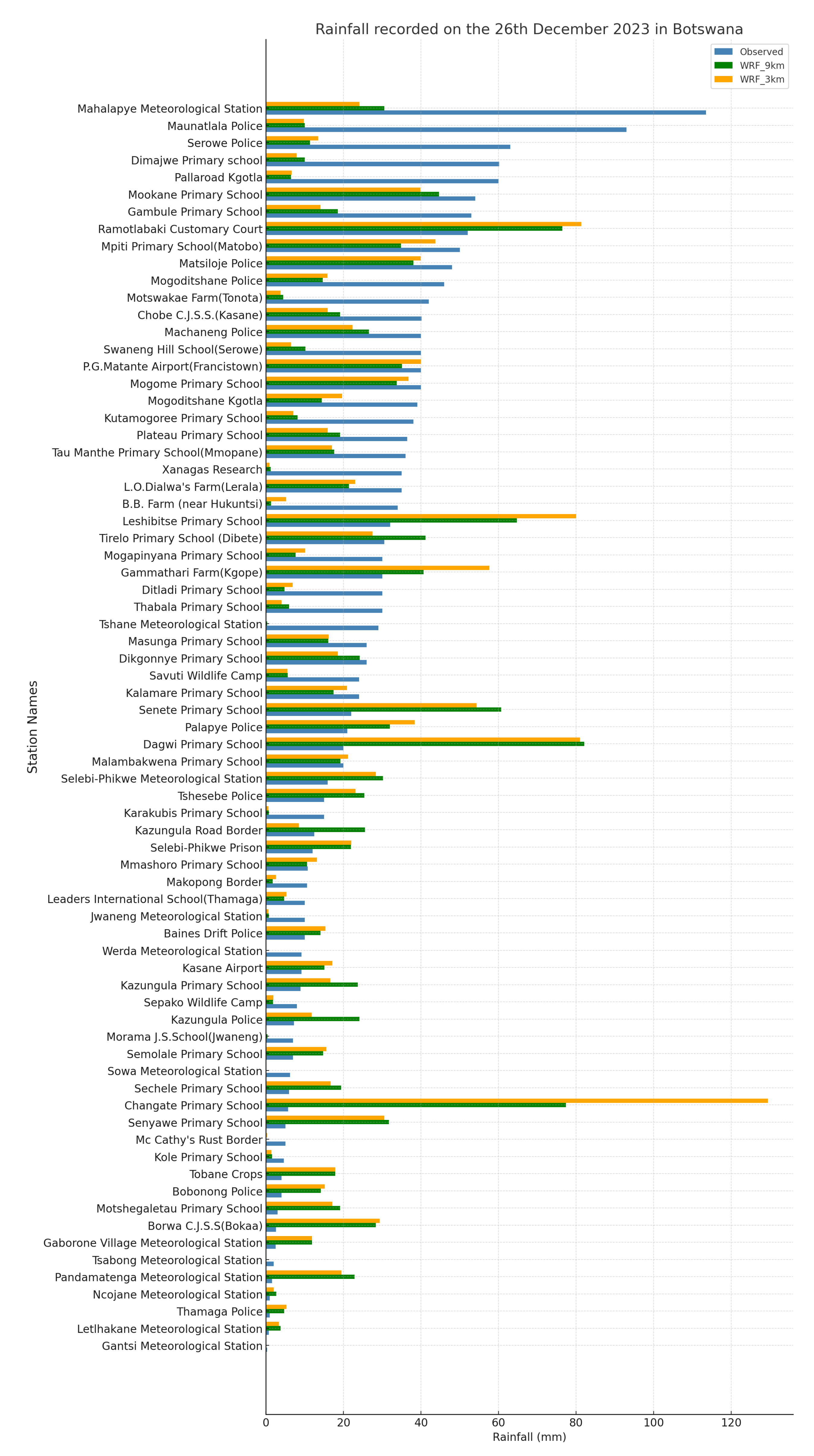
Figure 7 below shows the observed rainfall data from the network of DMS rain gauges at DMS. The data shows that rainfall was recorded for the 26th of December 2023. The highest amount of rainfall received was at Mahalapye Meteorological station (114 mm) and the lowest rainfall was received at Kalamare Primary School (24 mm) in Mahalapye District.
3.4. WRF Evaluation
The daily total rainfall estimates from ERA5 reanalysis and WRF model (Figure 8) show distinct differences in spatial distribution and intensity across southern Africa and specifically the Mahalapye District during the extreme rainfall event period of the 26th December 2023. ERA5 reanalysis data indicates that there was moderate rainfall in Mahalapye district (daily maximum below 20 mm). This may be highly attributed to the course resolution from ERA5 (approximately 31 km), which tends to underestimate localized convection and extreme rainfall magnitudes since it relies on parameterized convection and grid-scale averaging [38,41]. ERA5 dataset is primarily good at capturing the synoptic scale forcing which is associated with moisture inflow from the Indian ocean, but at times ERA5 outputs fails to explicitly resolve convective updrafts and storm structures at mesoscale level as outlined by [20,61].
In contrast, The WRF simulations at 9 km and 3 km resolutions produced a more improved representation of daily total rainfall during the period 26th December 2023. The 9 km WRF simulation shows an increased total rainfall with a maximum not exceeding 100 mm for the gauged stations at Mahalapye District. At the convection-permitting scale (3 km), the WRF model can explicitly resolve convective processes without the need for parameterization, but for this case the high resolution (3 km, d02) WRF simulation had reduced accuracy compared to the 9 km WRF setup. The main reason to the contrasting results from ERA5 reanalysis and WRF model simulations is the topography. WRF has better topography feedback as compared to ERA5 products because, ERA5 has reduced gradients over elevated terrain when compared to WRF. The WRF model, especially at high horizontal resolution is able to show close to reality topography and this is reflected in enhanced orographic lifting and convective, especially along slopes [62].
Figure 9 shows the Skew-T diagrams which were derived from the WRF model simulations, depicting vertical thermodynamic structure over the Mahalapye district on the 26th of December 2023 at around 14:00 UTC. The Skew T diagrams show pre-convective environment analysis from the gauged stations under investigation. In both d01 and d02, temperature (in red) and dew point (in green) profiles show a well-mixed boundary layer with a weak inversion near 850 - 700 hPa and strong drying 600 hPa. The structures displayed by in (Figure 9) are observed more often in continental tropical areas where mid-level subsidence and dry-air mixing have a big effect on convective formation. Figure 9 features are consistent with studies by [25,63], who found that southern Africa convection frequency develops beneath dry mid-tropospheric layers that control storm depth and lifetime.
At all the gauged station sites surface temperatures exceeded 28 – 320C, while dew point remained near 20 – 220C. This led to low-level dew point depressions of 3 – 50C and Lifted Condensation Level (LCL) between 712hPa and around 850 hPa (roughly 1.3 to 2 km). The low LCL heights suggests high-boundary-layer humidity and efficient cloud base formation especially over Machaneng, Mahalapye Meteorological station and Pallaroad Kgotla, where moisture advection from the northeast was the strongest. Above 700 hPa, dew-point lines diverge sharply from the temperature lines and showing a well defined dry layer that acts as a mixing barrier. This phenomenon of mid-level dryness tend to promote evaporative cooling in downdrafts, highlighted by [63,64] common on Botswana’s convective storms. Figure 9 concludes that the WRF model is in a position to show the vertical thermodynamics which contributed to the rainfall activity.
A list of all observed rainfall in Mahalapye District, obtained from BDMS against the WRF model run are shown in (Figure 10). The WRF model rainfall were interpolated using the Haversine and weighted average formula, at each station over Mahalapye district. The observations made from Pallaroad Kgotla and Mahalapye Meteorological Station were poorly simulated by WRF at both 9 and 3 km respectively (Figure 10). In theory, running WRF at 3 km offers a better grid-spacing and thus should yield better accuracy but in this study, it has been shown that for Mahalapye District WRF the 9 km run provided slightly better results as compared to the 3 km run. This has been observed in the validation statistics, although few stations were used in the verification process, which are unevenly distributed. It has also been shown in [11] that high resolution modelling produce better spatial distribution of meteorological variables including rainfall, but does not improve the statistics. Appendix Figure A1 shows total rainfall in Botswana on the 26th December 2023.
An interesting finding from the 9 km domain is that it slightly outperformed the 3 km model run in terms of the statistics including RMSE, correlation and the Kling-Gupta Efficiency (Table 4). The rule of thumb is that higher resolution simulations should yield better accuracy since the model will be able to resolve mesoscale processes [10,15]. Running WRF at 3 km recorded a PBIAS of -56.1%, while a 9 km run showed -48.2%, with both exhibiting negative KGE values (–0.356 and –0.225 respectively) and Pearson’s correlation coefficient (-0.038 and 0.020) close to zero to negative correlation with observed values. These findings confirm that WRF struggled with the intensity of rainfall simulation even under increased spatial resolution but managed to correctly capture the timing of rainfall events. The results from this study are supported by previous findings that resolution alone does not always guarantee improvement if model physics are not optimally configured [20,28]. Similar results were also reported by [23] in the upper Ganda Basin, where WRF’s higher-resolution run improved the timing of convection but did not enhance rainfall intensity estimates when evaluated against the eighteen (18) rain gauge stations in their study. For the case of Botswana, [28] found that the skill of WRF in simulating ex-tropical cyclone Dineo was dependent on the microphysics choices, with less sensitivity to model horizontal resolution. This strongly suggests that when it comes to local extreme events, studies should focus on model parameterization than model grid resolution/spacing.
The hypothesis for this study was as follows; can WRF, configured with the tropical-suite schemes and initialized with GFS forcing data, adequately reproduce the extreme rainfall event which occurred in Mahalapye District. The findings from the study supports this hypothesis: the WRF model was able to capture the broad-scale features and synoptic drivers, including the surface low-pressure system and mid-level trough that induced instability, which is in agreement with SAWS and GFS observed weather charts. From this study, we can strongly conclude that the model underestimation of rainfall totals points to limitations in cloud microphysics and cumulus parameterization. Studies by [21,23] highlighted that incorporating high-resolution microphysics and data assimilation can reduce these biases from the WRF model.
4. Summary and Conclusions
This study assessed the capability of WRF model in simulating an extreme rainfall event which occurred at Mahalapye District on 26thDecember 2023. The results show that WRF model run at 9 km and a 3 km nested domain is able to reproduce the spatial and temporal distribution of rainfall but with significant biases. The observed maximum rainfall recorded was 114 mm at Mahalapye Meteorological station, yet the WRF model simulations significantly underestimated its total rainfall. The findings of the study are consistent with earlier work from other authors including [23,48], thus indicating that WRF frequently underestimates extreme rainfall magnitudes. However, the model was able to capture spatial distribution of rainfall reasonably well.
Besides bias, both domains achieved a good probability of detection (POD = 1.00), indicating that the WRF model effectively identified the occurrence of rainfall. A high POD value indicates that the models’ ability to capture rainfall timing and location is impressive, which is epecially important in applications of early warning [52]. Considering WRF model bias, the negative bias values (-56.1% to -48.2% for WRF at 3 km and 9 km respectively) highlights the models’ systematic underestimation of rainfall which was also observed over stations in Lagos by [48] and in southern Africa by [20]. These findings strongly suggest that the models’ tropical-suite physics configuration captures convective activities during their initiation but struggles to sustain rainfall intensities.
The implications of this study’s findings extend to flood risk management and disaster preparedness in Botswana. Flooding episodes in the country of Botswana are becoming more frequent, with increasing socio-economic impacts [3,4]. This could be due to the impacts of climate change and variability [37]. This study confirms that dynamical downscaling with WRF provides valuable predictive information on extreme rainfall but highlights the necessity of model customization for local conditions. The WRF models’ systematic biases identified in this study, reinforce the importance of ensemble-based sensitivity testing to provide probabilistic guidance and suggested in African regional studies [12,48].
In conclusion, future research should focus on multi-physics ensemble simulations, data assimilation of local BDMS observations and coupling WRF outputs with hydrological models to directly forecast flash floods magnitudes and its associated impacts. Furthermore, extending validation beyond a single event to multiple case studies would also provide more robust assessment of WRF’s reliability across varying synoptic conditions.
Author Contributions
K.C.M. conceptualized the study, designed the methodology, implemented the WRF setup and associated post-processing software, curated the data, and performed the validation and formal analyses with technical input from G.R. K.C.M also produced the visualizations and prepared the original draft. T.R.M provided high-level supervision, offering expert guidance on numerical modeling and interpretation of results alongside K.M and M.W. contributed to the overall supervision of the work. T.R.M, K.M, and M.W reviewed and refined the text and also ensured that the paper has scientific clarity. All authors have read and agreed to the published version of the manuscript
Funding
This research received no external funding.
Institutional Review Board Statement
Not Applicable.
Data Availability Statement
Not Applicable.
Appendix A.
Figure A1.
Rainfall recorded on the 26th December 2023 across all stations in Botswana.
References
- McPhillips, L.E.; Chang, H.; Chester, M.V.; Depietri, Y.; Friedman, E.; Grimm, N.B.; Kominoski, J.S.; McPhearson, T.; Méndez-Lázaro, P.; Rosi, E.J.; et al. Defining extreme events: A cross-disciplinary review. *Earth’s Future* **2018**, *6*(3), 441–455. [CrossRef]
- Batisani, N.; Yarnal, B. Rainfall variability and trends in semi-arid Botswana: Implications for climate change adaptation policy. *Applied Geography* **2010**, *30*(4), 483–489. [CrossRef]
- Statistics Botswana. *Botswana Environment Statistics: Natural and Technological Disasters Digest 2019*; Statistics Botswana: Gaborone, Botswana, 2020.
- Mmopelwa, G.; Moalafhi, D.B.; Hambira, W.L.; Dhliwayo, M.; Motau, A. The impact of flooding on the community: A case of Gweta and Zoroga Villages, Botswana. *African Journal of Climate Change and Resource Sustainability* **2023**, *2*(1), 132–152. [CrossRef]
- Motsholapheko, M.R.; Kgathi, D.L.; Vanderpost, C. Rural livelihoods and household adaptation to extreme flooding in the Okavango Delta, Botswana. *Physics and Chemistry of the Earth, Parts A/B/C* **2011**, *36*(14–15), 984–995. [CrossRef]
- Tsheko, R. Rainfall reliability, drought and flood vulnerability in Botswana. *Water SA* **2003**, *29*(4), 389–392. [CrossRef]
- Samuel, G.; Mulalu, M.I.; Moalafhi, D.B.; Stephens, M. Evaluation of national disaster management strategy and planning for flood management and impact reduction in Gaborone, Botswana. *International Journal of Disaster Risk Reduction* **2022**, *74*, 102939. [CrossRef]
- Moses, O. Weather systems influencing Botswana rainfall: The case of 9 December 2018 storm in Mahalapye, Botswana. *Modeling Earth Systems and Environment* **2019**, *5*(4), 1473–1480. [CrossRef]
- Aravind, A.; Srinivas, C.V.; Hegde, M.N.; Seshadri, H.; Mohapatra, D.K. Impact of land surface processes on the simulation of sea breeze circulation and tritium dispersion over the Kaiga complex terrain region near west coast of India using the Weather Research and Forecasting (WRF) model. *Atmospheric Environment: X* **2022**, *13*, 100149. [CrossRef]
- Giorgi, F. Simulation of regional climate using a limited area model nested in a general circulation model. *Journal of Climate* **1990**, *3*(9), 941–963. [CrossRef]
- Maisha, T.R. The Influence of Topography and Model Grid Resolution on Extreme Weather Forecasts over South Africa. Ph.D. Thesis, University of Pretoria, Pretoria, South Africa, 2014.
- Reason, C.J.C.; Landman, W.; Tennant, W. Seasonal to decadal prediction of southern African climate and its links with variability of the Atlantic Ocean. *Bulletin of the American Meteorological Society* **2006**, *87*(7), 941–956. [CrossRef]
- Giorgi, F. Regional climate modeling: Status and perspectives. *Journal de Physique IV (Proceedings)* **2006**, *139*, 101–118. [CrossRef]
- Kgatuke, M.M.; Landman, W.A.; Beraki, A.; Mbedzi, M.P. The internal variability of the RegCM3 over South Africa. *International Journal of Climatology: A Journal of the Royal Meteorological Society* **2008**, *28*(4), 505–520. [CrossRef]
- Feser, F.; Rockel, B.; von Storch, H.; Winterfeldt, J.; Zahn, M. Regional climate models add value to global model data: a review and selected examples. *Bulletin of the American Meteorological Society* **2011**, *92*(9), 1181–1192. [CrossRef]
- Xu, Z.; Han, Y.; Yang, Z. Dynamical downscaling of regional climate: A review of methods and limitations. *Science China Earth Sciences* **2019**, *62*, 365–375. [CrossRef]
- Rummukainen, M. State-of-the-art with regional climate models. *Wiley Interdisciplinary Reviews: Climate Change* **2010**, *1*(1), 82–96.
- Wang, Y.; Leung, L.R.; McGregor, J.L.; Lee, D.K.; Wang, W.C.; Ding, Y.; Kimura, F. Regional climate modeling: Progress, challenges, and prospects. *Journal of the Meteorological Society of Japan. Ser. II* **2004**, *82*(6), 1599–1628. [CrossRef]
- Skamarock, W.C.; Klemp, J.B.; Dudhia, J.; Gill, D.O.; Liu, Z.; Berner, J.; Wang, W.; Powers, J.G.; Duda, M.G.; Barker, D.M.; et al. A Description of the Advanced Research WRF Version 4; NCAR Technical Note NCAR/TN-556+STR; National Center for Atmospheric Research: Boulder, CO, USA, 2019.
- Ratna, S.B.; Ratnam, J.V.; Behera, S.K.; Rautenbach, C.J.d.W.; Ndarana, T.; Takahashi, K.; Yamagata, T. Performance assessment of three convective parameterization schemes in WRF for downscaling summer rainfall over South Africa. *Climate Dynamics* **2014**, *42*, 2931–2953. [CrossRef]
- Mazzoglio, P.; Parodi, A.; Parodi, A. Detecting Extreme Rainfall Events Using the WRF-ERDS Workflow: The 15 July 2020 Palermo Case Study. *Water* **2022**, *14*(1), 86.
- Bafitlhile, T.M.; Oladele, A.S. Modeling Extreme Flood Events for Palapye, Botswana. *BIE Journal of Engineering and Applied Sciences* **2015**, *6*(1), 54–60.
- Chawla, I.; Osuri, K.K.; Mujumdar, P.P.; Niyogi, D. Assessment of the Weather Research and Forecasting (WRF) model for simulation of extreme rainfall events in the upper Ganga Basin. *Hydrology and Earth System Sciences* **2018**, *22*(2), 1095–1117. [CrossRef]
- Sun, B.-Y.; Bi, X.-Q. Validation for a tropical belt version of WRF: Sensitivity tests on radiation and cumulus convection parameterizations. *Atmospheric and Oceanic Science Letters* **2019**, *12*(3), 192–200. [CrossRef]
- Meroni, A.N.; Oundo, K.A.; Muita, R.; Bopape, M.-J.; Maisha, T.R.; Lagasio, M.; Parodi, A.; Venuti, G. Sensitivity of some African heavy rainfall events to microphysics and planetary boundary layer schemes: Impacts on localised storms. *Quarterly Journal of the Royal Meteorological Society* **2021**, *147*(737), 2448–2468. [CrossRef]
- Mofokeng, P.S. Study of the influence of gust fronts and topographical features in the development of severe thunderstorms across South Africa. *University of the Witwatersrand, Johannesburg* **2024**.
- Maisha, T.; Mulovhedzi, P.T.; Rambuwani, G.T.; Makgati, L.N.; Barnes, M.; Lekoloane, L.; Engelbrecht, F.A.; Ndarana, T.; Mbokodo, I.L.; Xulu, N.G.; et al. The development of a locally based weather and climate model in Southern Africa. *Water Research Commission: Pretoria, South Africa* **2025**, 1–197.
- Molongwane, C.; Bopape, M.-J.M.; Fridlind, A.; Motshegwa, T.; Matsui, T.; Phaduli, E.; Sehurutshi, B.; Maisha, R. Sensitivity of Botswana Ex-Tropical Cyclone Dineo rainfall simulations to cloud microphysics scheme. *AAS Open Research* **2020**, *3*, 30. [CrossRef]
- Mathafeni, T.P.; Osupile, O.; Maripe, K. Hazard Early Warning Systems in Botswana: A Social Work Perspective. *International Journal of Health and Medical Information* **2015**, *4*(1), 9–22.
- Statistics Botswana. Botswana Population and Housing Census 2022. *Government of Botswana Publications* **2022**. Accessed via Botswana Bureau of Statistics.
- Kumar, P.; Kishtawal, C.M.; Pal, P.K. Impact of ECMWF, NCEP, and NCMRWF global model analysis on the WRF model forecast over Indian Region. *Theoretical and Applied Climatology* **2017**, *127*, 143–151. [CrossRef]
- Taszarek, M.; Pilguj, N.; Orlikowski, J.; Surowiecki, A.; Walczakiewicz, S.; Pilorz, W.; Piasecki, K.; Pajurek, Ł.; Półrolniczak, M. Derecho evolving from a mesocyclone—A study of 11 August 2017 severe weather outbreak in Poland: Event analysis and high-resolution simulation. *Monthly Weather Review* **2019**, *147*(6), 2283–2306. [CrossRef]
- Figurski, M.J.; Nykiel, G.; Jaczewski, A.; Bałdysz, Z.; Wdowikowski, M. The impact of initial and boundary conditions on severe weather event simulations using a high-resolution WRF model. Case study of the derecho event in Poland on 11 August 2017. *Meteorology Hydrology and Water Management. Research and Operational Applications* **2022**, *10*. [CrossRef]
- Nkoni, G.; Mphale, K.; Mbangiwa, N.; Samuel, S.; Molosiwa, R. Use of multivariate techniques to regionalize rainfall patterns in semiarid Botswana. *Discover Environment* **2024**, *2*(1), 77. [CrossRef]
- Alemaw, B.F.; Chaoka, R.T. ; Others. Regionalization of rainfall intensity-duration-frequency (IDF) curves in Botswana. *Journal of Water Resource and Protection* **2016**, *8*(12), 1128. [CrossRef]
- Akinyemi, F.O. Climate change and variability in semiarid Palapye, Eastern Botswana: An assessment from smallholder farmers’ perspective. *Weather, Climate, and Society* **2017**, *9*(3), 349–365. [CrossRef]
- Matenge, R.G.; Parida, B.P.; Letshwenyo, M.W.; Ditalelo, G. Impact of climate variability on rainfall characteristics in the semi-arid Shashe Catchment (Botswana) from 1981–2050. *Earth* **2023**, *4*(2), 398–441. [CrossRef]
- Hersbach, H.; Bell, B.; Berrisford, P.; Hirahara, S.; Horányi, A.; Muñoz-Sabater, J.; Nicolas, J.; Peubey, C.; Radu, R.; Schepers, D.; et al. *The ERA5 Global Reanalysis*; *Quarterly Journal of the Royal Meteorological Society* **2020**, *146*(730), 1999–2049. Wiley Online Library. [CrossRef]
- Mbokodo, I.L.; Burger, R.P.; Fridlind, A.; Ndarana, T.; Maisha, R.; Chikoore, H.; Bopape, M.-J.M. *Assessing the Performance of the WRF Model in Simulating Squall Line Processes over the South African Highveld*; *Atmosphere* **2025**, *16*(9), 1055. MDPI. [CrossRef]
- Bopape, M.-J.M.; Engelbrecht, F.A.; Maisha, R.; Chikoore, H.; Ndarana, T.; Lekoloane, L.; Thatcher, M.; Mulovhedzi, P.T.; Rambuwani, G.T.; Barnes, M.A.; et al. *Rainfall Simulations of High-Impact Weather in South Africa with the Conformal Cubic Atmospheric Model (CCAM)*; *Atmosphere* **2022**, *13*(12), 1987. MDPI. [CrossRef]
- Dee, D.P.; Uppala, S.M.; Simmons, A.J.; Berrisford, P.; Poli, P.; Kobayashi, S.; Andrae, U.; Balmaseda, M.A.; Balsamo, G.; Bauer, P.; et al. *The ERA-Interim Reanalysis: Configuration and Performance of the Data Assimilation System*; *Quarterly Journal of the Royal Meteorological Society* **2011**, *137*(656), 553–597. Wiley Online Library. [CrossRef]
- Steinkopf, J.; Engelbrecht, F. *Verification of ERA5 and ERA-Interim Precipitation over Africa at Intra-Annual and Interannual Timescales*; *Atmospheric Research* **2022**, *280*, 106427. Elsevier. [CrossRef]
- Wang, W. WRF: More Runtime Options. *WRF Tutorial* **2017**, *46*, UNSW Sydney, NSW, Australia.
- Iacono, M.J.; Delamere, J.S.; Mlawer, E.J.; Shephard, M.W.; Clough, S.A.; Collins, W.D. Radiative forcing by long-lived greenhouse gases: Calculations with the AER radiative transfer models. *J. Geophys. Res. Atmos.* **2008**, *113*, D13. [CrossRef]
- Hong, S.-Y.; Noh, Y.; Dudhia, J. A new vertical diffusion package with an explicit treatment of entrainment processes. *Mon. Weather Rev.* **2006**, *134*, 2318–2341. [CrossRef]
- Tewari, M. Implementation and Verification of the Unified NOAH Land Surface Model in the WRF Model. 2004. Available online: https://ral.ucar.edu/projects/wrf/users/docs/WRF-ARWPhysiology.pdf (accessed on 18 May 2024).
- Zhang, C.; Wang, Y. Projected future changes of tropical cyclone activity over the western North and South Pacific in a 20-km-mesh regional climate model. *J. Clim.* **2017**, *30*, 5923–5941. [CrossRef]
- Oyegbile, O.; Chan, A.; Ooi, M.; Anwar, P.; Mohamed, A.A.; Li, L. Evaluation of WRF model performance with different microphysics schemes for extreme rainfall prediction in Lagos, Nigeria: Implications for urban flood risk management. *Bull. Atmos. Sci. Technol.* **2024**, *5*, 19. [CrossRef]
- Chai, T.; Draxler, R.R. Root mean square error (RMSE) or mean absolute error (MAE)?—Arguments against avoiding RMSE in the literature. *Geosci. Model Dev.* **2014**, *7*, 1247–1250. [CrossRef]
- Moriasi, D.; Arnold, J.; Van Liew, M.; Bingner, R.; Harmel, R.D.; Veith, T. Model Evaluation Guidelines for Systematic Quantification of Accuracy in Watershed Simulations. *Trans. ASABE* **2007**, *50*, 885–900. [CrossRef]
- Legates, D.R.; McCabe, G.J. Evaluating the use of “goodness-of-fit” measures in hydrologic and hydroclimatic model validation. *Water Resour. Res.* **1999**, *35*, 233–241.
- Wilks, D.S. *Statistical Methods in the Atmospheric Sciences*, 3rd ed.; Academic Press: Oxford, UK, 2011; Volume 100, International Geophysics Series.
- Gupta, H.; Kling, H.; Yilmaz, K.; Martinez, G. Decomposition of the Mean Squared Error and NSE Performance Criteria: Implications for Improving Hydrological Modelling. *J. Hydrol.* **2009**, *377*, 80–91. [CrossRef]
- Mass, C.F.; Ovens, D.; Westrick, K.; Colle, B.A. Does Increasing Horizontal Resolution Produce More Skillful Forecasts? The Results of Two Years of Real-Time Numerical Weather Prediction over the Pacific Northwest. *Bull. Am. Meteorol. Soc.* **2002**, *83*, 407–430.
- Jiménez, P.; Dudhia, J. Improving the Representation of Resolved and Unresolved Topographic Effects on Surface Wind in the WRF Model. *J. Appl. Meteorol. Climatol. 2012. [Google Scholar] [CrossRef]
- Farr, T.G.; Rosen, P.A.; Caro, E.; Crippen, R.; Duren, R.; Hensley, S.; Kobrick, M.; Paller, M.; Rodriguez, E.; Roth, L.; et al. The Shuttle Radar Topography Mission (SRTM). *Reviews of Geophysics* **2007**, *45*(2), RG2004. [CrossRef]
- Lehner, B.; Verdin, K.; Jarvis, A. New global hydrography derived from spaceborne elevation data. *Eos, Transactions American Geophysical Union* **2008**, *89*(10), 93–94. [CrossRef]
- McSweeney, C.F.; Jones, R.G.; Lee, R.W.; Rowell, D.P. *Selecting CMIP5 GCMs for Downscaling over Multiple Regions*; *Climate Dynamics* **2015**, *44*(11), 3237–3260. Springer. [CrossRef]
- Dyson, L.L.; Van Heerden, J.; Sumner, P.D. *A Baseline Climatology of Sounding-Derived Parameters Associated with Heavy Rainfall over Gauteng, South Africa*; *International Journal of Climatology* **2015**, *35*(7), 1162–1174. Wiley. [CrossRef]
- Van Schalkwyk, L.; Blamey, R.C.; Dyson, L.L.; Reason, C.J.C. *A Climatology of Drylines in the Interior of Subtropical Southern Africa*; *Journal of Climate* **2022**, *35*(19), 6411–6430. [CrossRef]
- Blamey, R.C.; Reason, C.J.C. *Mesoscale Convective Complexes over Southern Africa*; *Journal of Climate* **2012**, *25*(2), 753–766. [CrossRef]
- Dedekind, Z.; Engelbrecht, F.A.; Van der Merwe, J. *Model Simulations of Rainfall over Southern Africa and Its Eastern Escarpment*; *Water SA* **2016**, *42*(1), 129–143. [CrossRef]
- Crétat, J.; Pohl, B.; Richard, Y.; Drobinski, P. Uncertainties in simulating regional climate of Southern Africa: Sensitivity to physical parameterizations using WRF. *Clim. Dyn.* **2012**, *38*(3), 613–634. [CrossRef]
- Engelbrecht, F.A.; McGregor, J.L.; Engelbrecht, C.J. Dynamics of the Conformal-Cubic Atmospheric Model projected climate-change signal over southern Africa. *Int. J. Climatol.* **2009**, *29*(7), 1013–1033. [CrossRef]
Figure 1.
Study area showing the geographical location of the study area and the location of gauged stations (black dots).
Figure 1.
Study area showing the geographical location of the study area and the location of gauged stations (black dots).
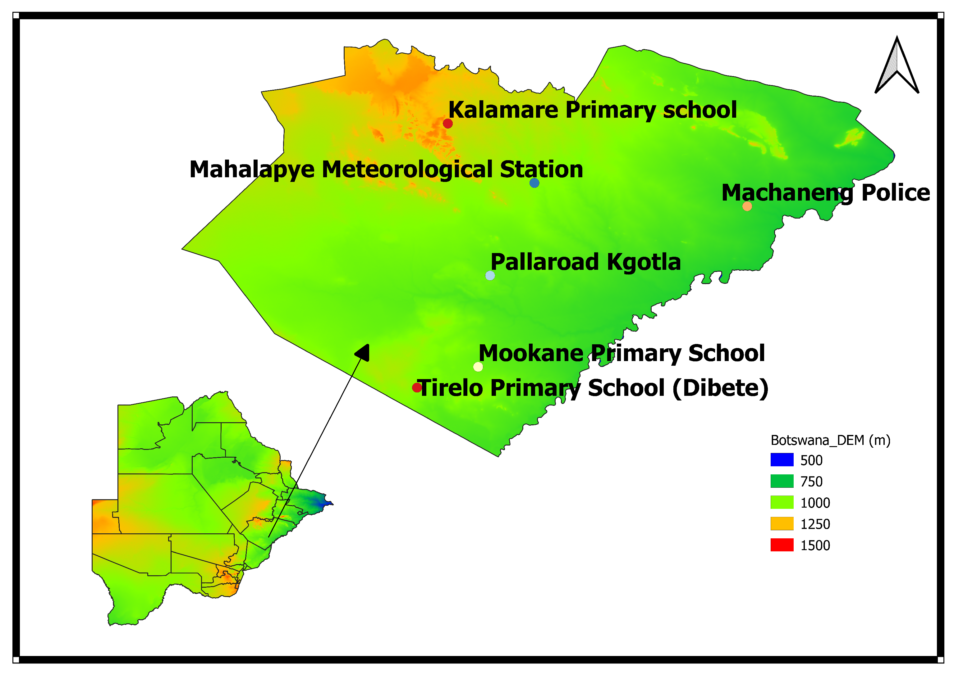
Figure 2.
WRF model domain setup showing the parent domain at 9 km with a nested domain at 3 km, centered over Botswana.
Figure 2.
WRF model domain setup showing the parent domain at 9 km with a nested domain at 3 km, centered over Botswana.
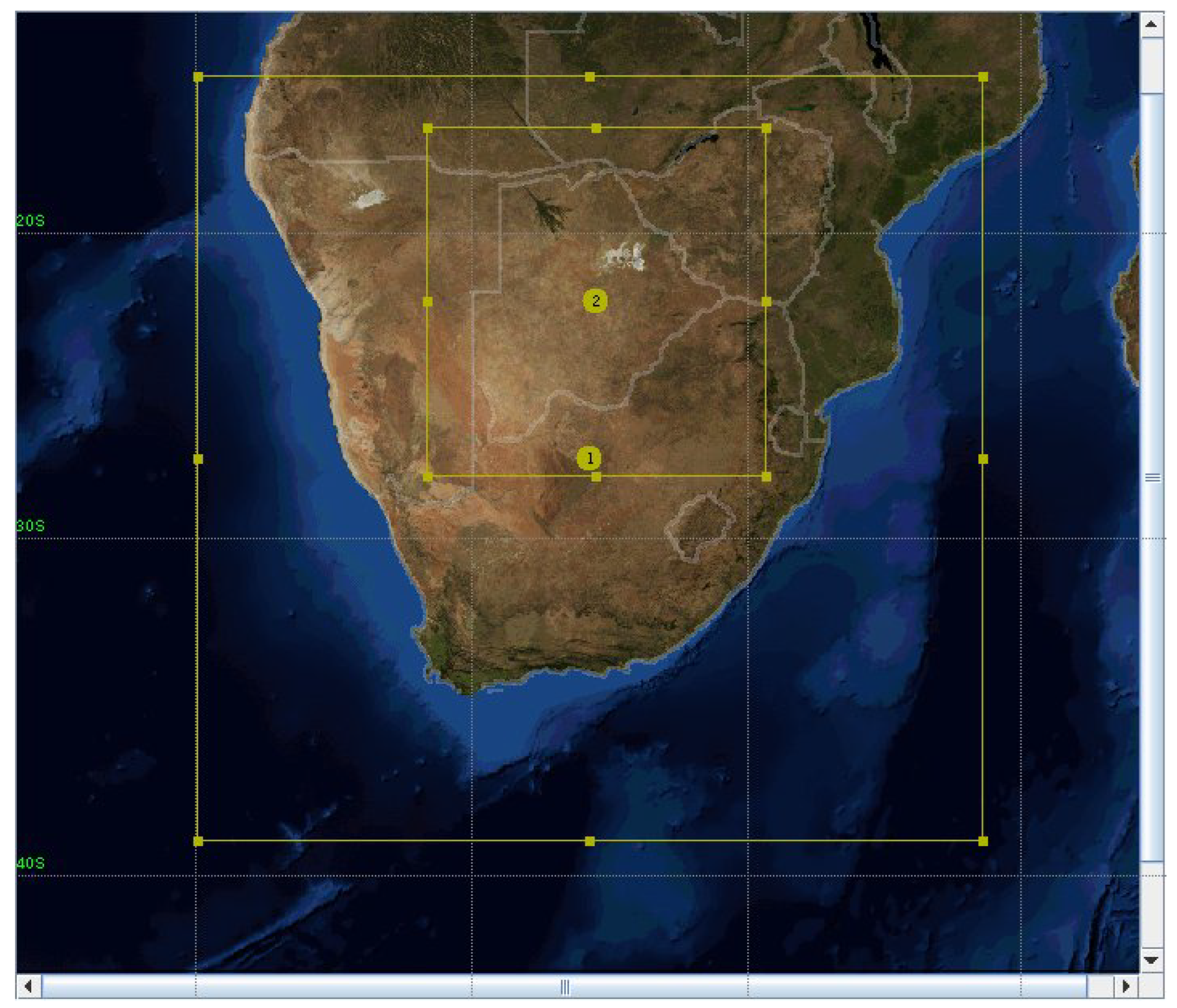
Figure 3.
SRTM Digital Elevation Model (DEM), ERA5, and WRF showing the elevation gradient across Botswana.
Figure 3.
SRTM Digital Elevation Model (DEM), ERA5, and WRF showing the elevation gradient across Botswana.
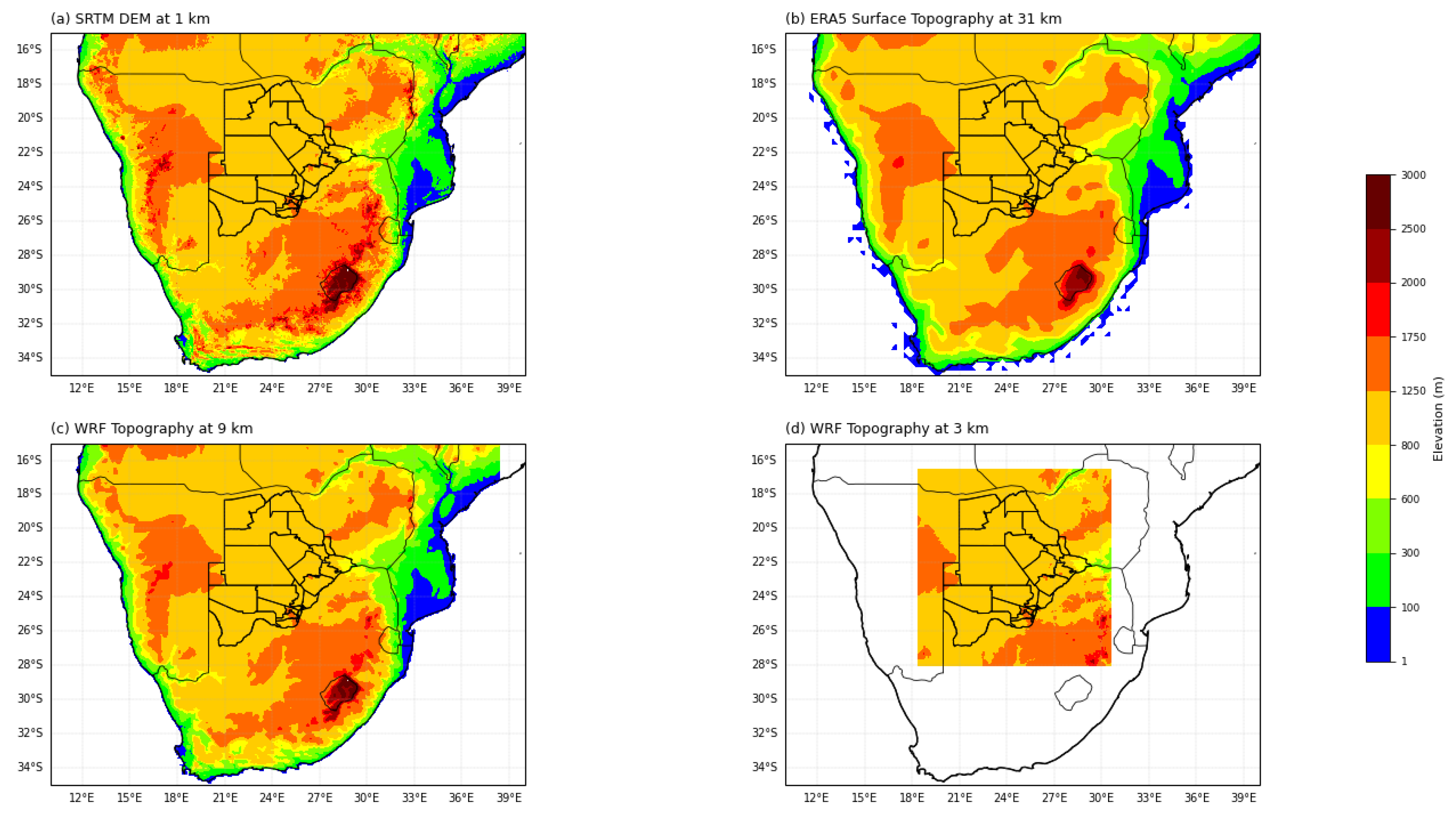
Figure 4.
Comparison of synoptic weather charts from SAWS (left) and GFS (right) for 26th December 2023.
Figure 4.
Comparison of synoptic weather charts from SAWS (left) and GFS (right) for 26th December 2023.
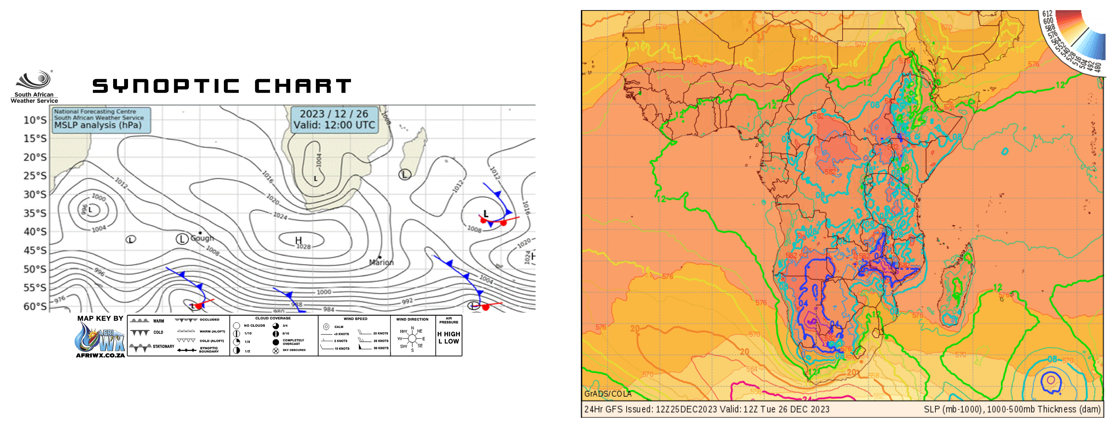
Figure 5.
Spatial distribution of relative humidity (RH) and wind vectors at 800 hPa and 500 hPa from (a–b) ERA5, (c–d) WRF d01 (9 km), and (e–f) WRF d02 (3 km) simulations on 26th December 2023 (12:00 UTC). The red outline marks Mahalapye District.
Figure 5.
Spatial distribution of relative humidity (RH) and wind vectors at 800 hPa and 500 hPa from (a–b) ERA5, (c–d) WRF d01 (9 km), and (e–f) WRF d02 (3 km) simulations on 26th December 2023 (12:00 UTC). The red outline marks Mahalapye District.
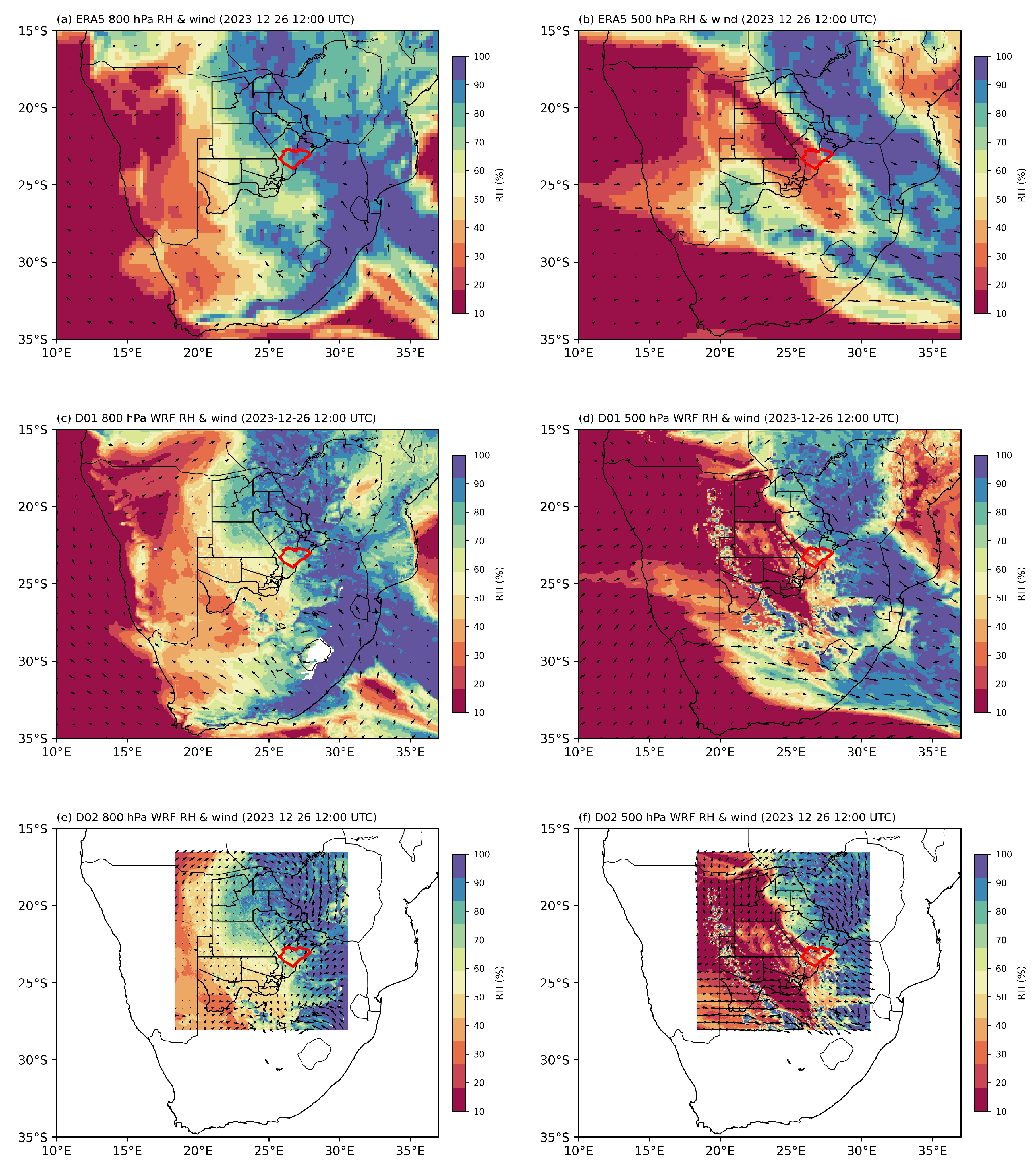
Figure 6.
GFS 500 mb geopotential height and vorticity (left), and 24-hour accumulated precipitation on 26th December 2023 at 12:00 UTC (right).
Figure 6.
GFS 500 mb geopotential height and vorticity (left), and 24-hour accumulated precipitation on 26th December 2023 at 12:00 UTC (right).
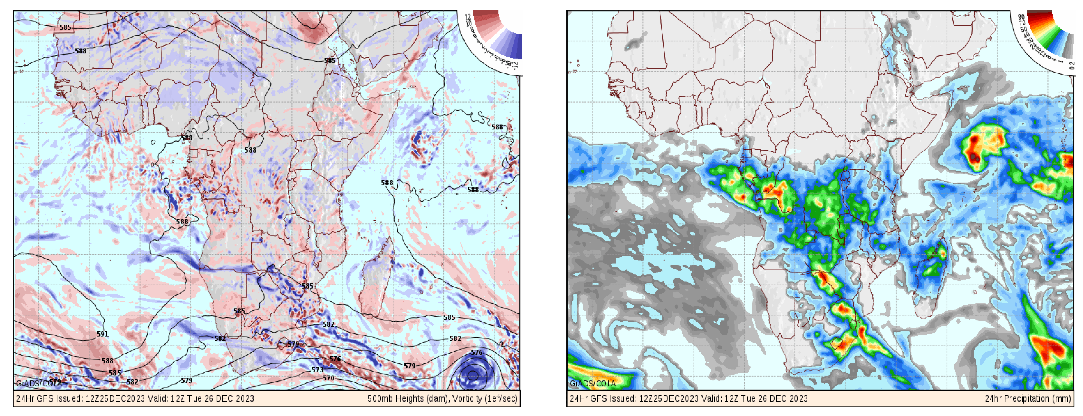
Figure 7.
Observed rainfall from BDMS gauged stations across Mahalapye District.
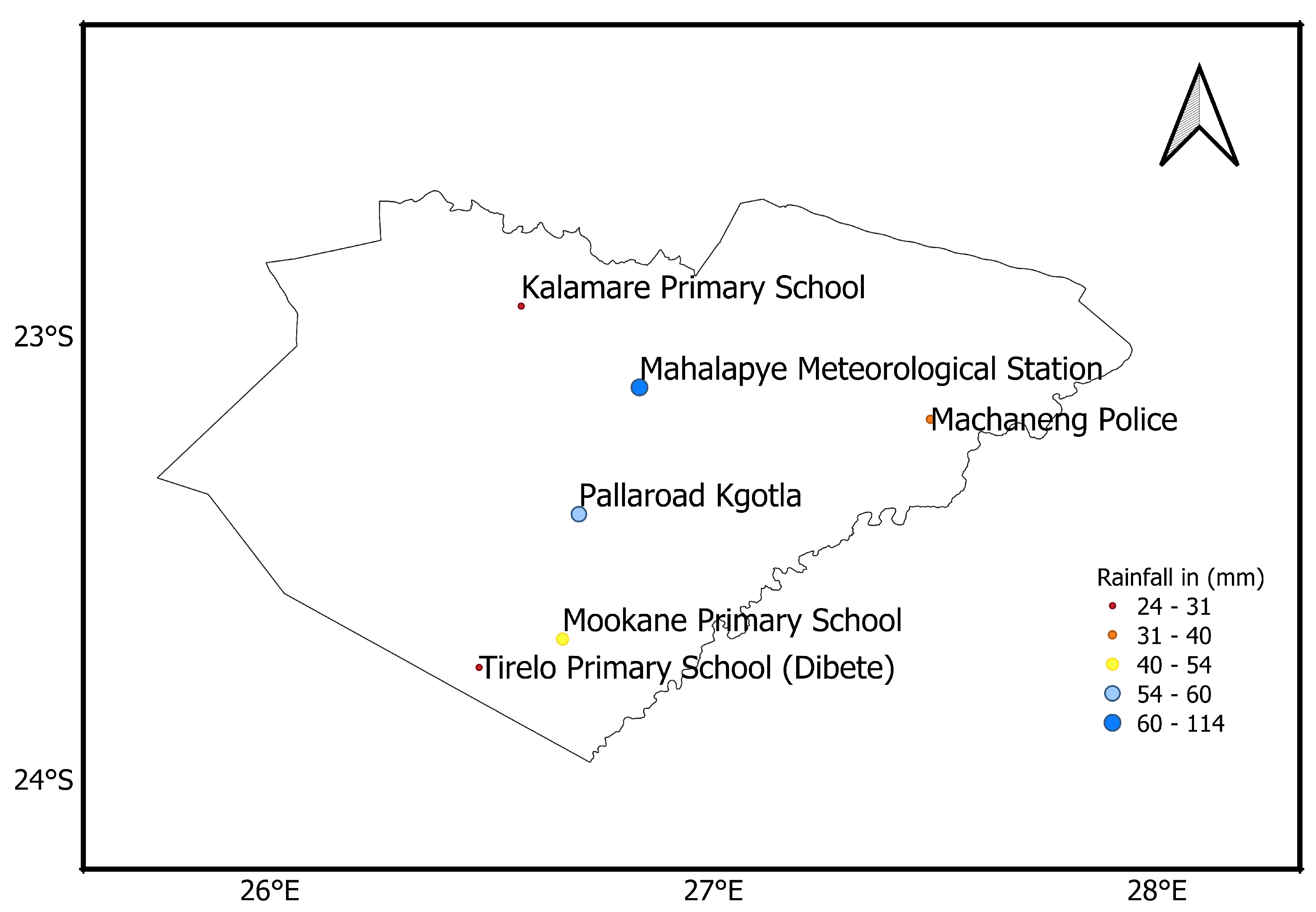
Figure 8.
ERA5 (left), WRF 9 km resolution (middle) and WRF 3 km resolution (right) for Mahalapye District.
Figure 8.
ERA5 (left), WRF 9 km resolution (middle) and WRF 3 km resolution (right) for Mahalapye District.
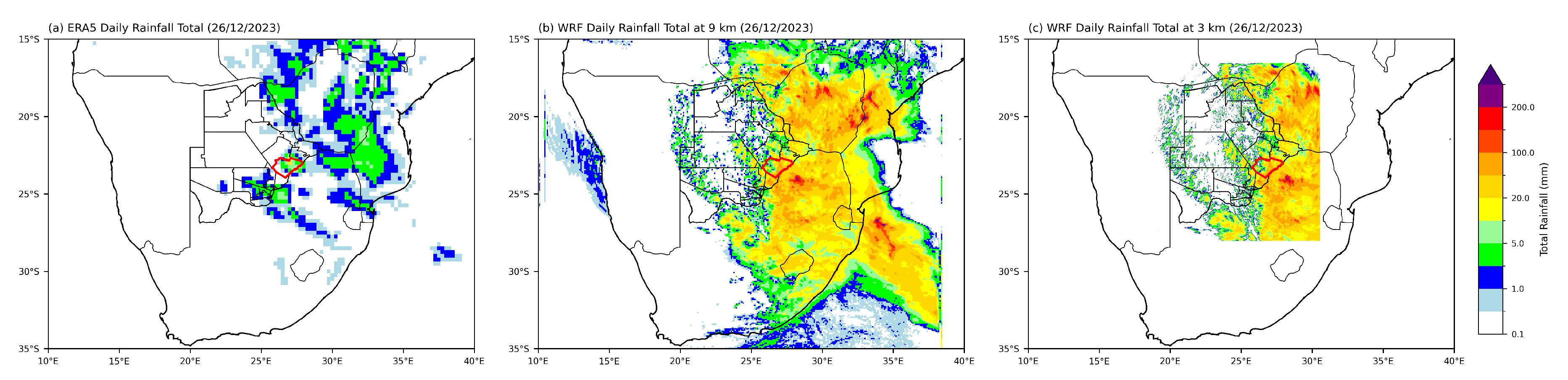
Figure 9.
Simulated Skew-T log-p diagrams from WRF simulations on 26 December 2023 (12:00 UTC). Rows 1–2: Domain 1 (9 km); Rows 3–4: Domain 2 (3 km). Temperature (red), dewpoint (green), and wind barbs illustrate thermodynamic and kinematic structure across six stations (Kalamare, Machaneng, Mahalapye, Mookane, Pallaroad, and Tirelo).
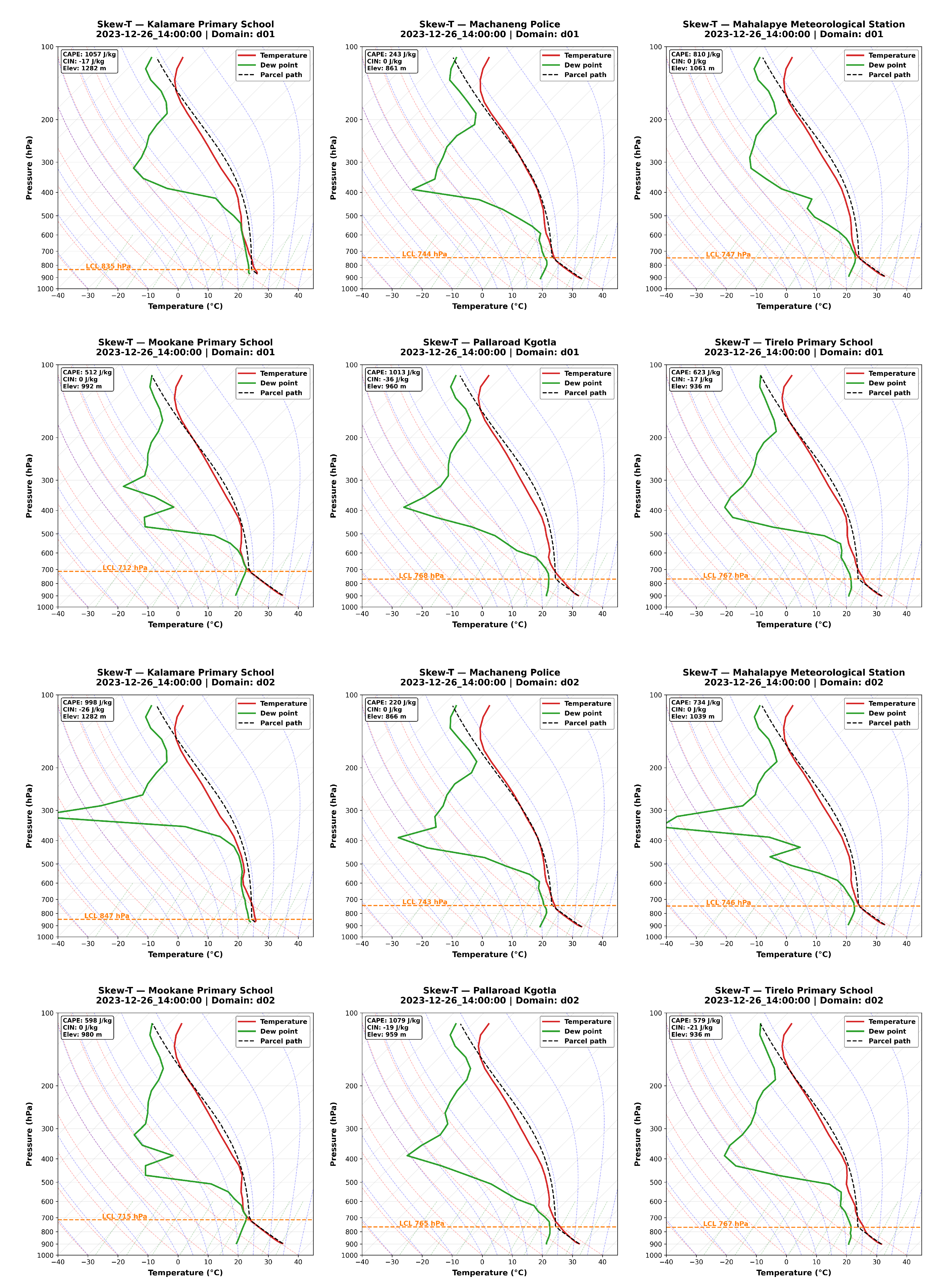
Figure 10.
Mahalapye District WRF simulation outputs.
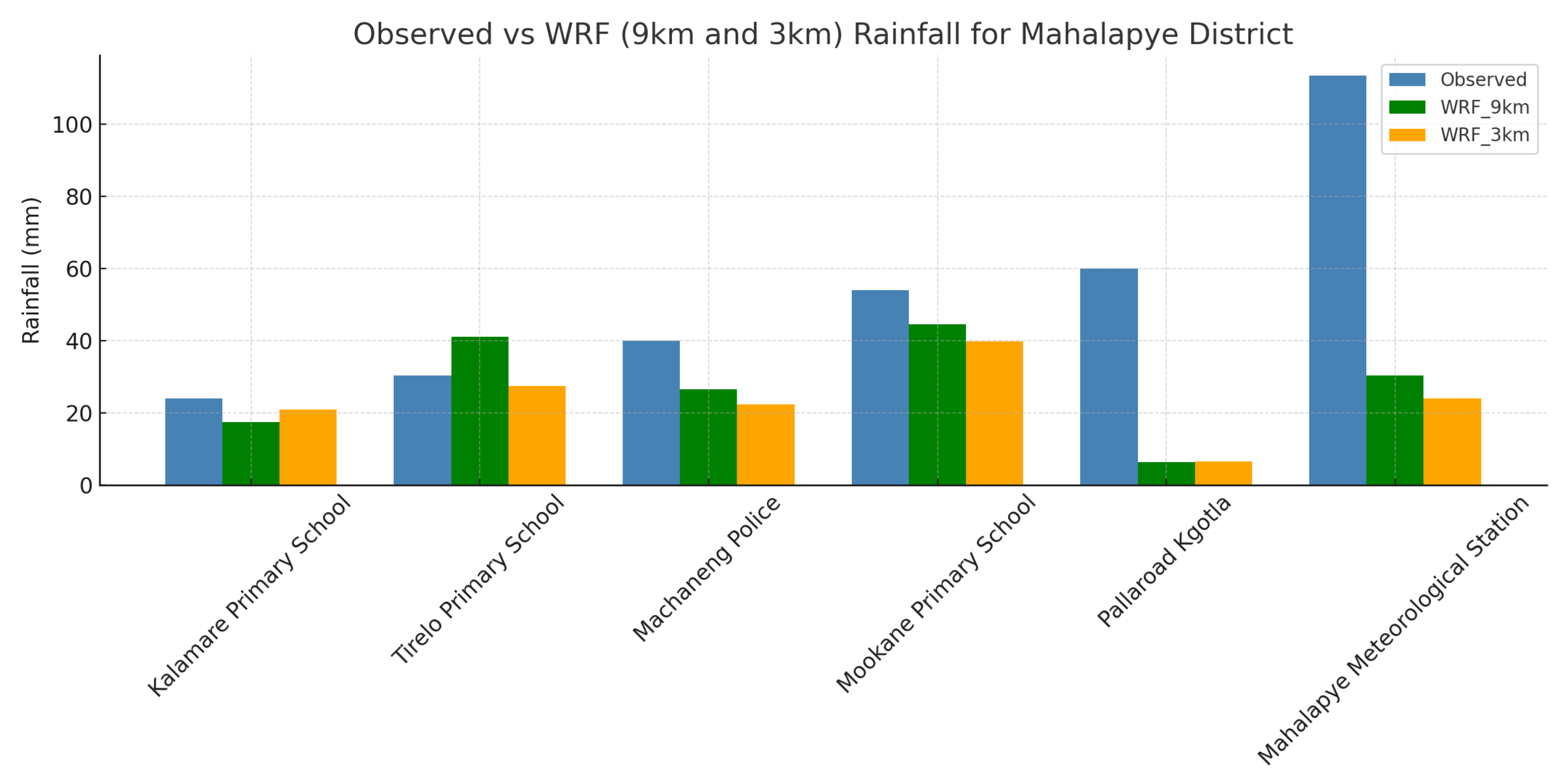

Table 1.
Station names used in Mahalapye District.
| Station Name | Lat | Lon | Altitude (m) |
|---|---|---|---|
| Mahalapye Meteorological Station | S | E | 1017 |
| Mookane Primary School | S | E | 951 |
| Tirelo Primary School | S | E | 957 |
| Kalamare Primary School | S | E | 1074 |
| Machaneng Police | S | E | 888 |
| Pallaroad Kgotla | S | E | 1002 |
Table 2.
WRF model configuration for simulation of heavy rainfall event.
| Model Options | Specifications |
|---|---|
| Model type | Non-hydrostatic |
| Domains | two (2) (with a two-way nested domains) |
| Grid resolution (spacing) | parent domain 1: 9 km × 9 km; (312 × 301 grid) |
| nested domain 2: 3 km × 3 km; (403 × 412 grid) | |
| Map projection | Mercator |
| Initial conditions | NCEP GFS (3 hourly interval) |
| PBL Schemes | YSU scheme |
| Cumulus schemes | A newer Tiedtke scheme |
| Microphysics schemes | WSM 6-class graupel scheme |
| Shortwave radiation scheme | RRTMG scheme |
| Longwave radiation scheme | RRTMG scheme |
| Land surface model | Unified Noah land surface model |
Table 3.
WRF Tropical Suite physics schemes.
| Scheme | Description |
|---|---|
| RRTM | Rapid Radiative Transfer Model used to improve radiative transfer |
| calculations during the WRF run; developed by [44]. | |
| YSU | Yonsei University planetary boundary layer scheme introduced by |
| [45]; represents boundary layer processes. | |
| Noah LSM | Unified Noah land surface model used to capture land surface |
| interactions; developed by [46]. | |
| New Tiedtke | Updated cumulus scheme by [47]; used in |
| cumulus convection representation. | |
| WSM6 | Weather Research and Forecasting Single-Moment 6-class |
| microphysics scheme developed by [45]; | |
| provides detailed microphysical processes. |
Table 4.
Performance metrics for WRF simulations on the 26th of December 2023 over Mahalapye District.
Table 4.
Performance metrics for WRF simulations on the 26th of December 2023 over Mahalapye District.
| Model | RMSE (mm) | PBIAS (%) | KGE | r | POD (1 mm) |
|---|---|---|---|---|---|
| WRF_3km | 43.529 | -56.10 | -0.356 | -0.038 | 1.000 |
| WRF_9km | 41.197 | -48.22 | -0.225 | 0.020 | 1.000 |
Disclaimer/Publisher’s Note: The statements, opinions and data contained in all publications are solely those of the individual author(s) and contributor(s) and not of MDPI and/or the editor(s). MDPI and/or the editor(s) disclaim responsibility for any injury to people or property resulting from any ideas, methods, instructions or products referred to in the content. |
© 2025 by the authors. Licensee MDPI, Basel, Switzerland. This article is an open access article distributed under the terms and conditions of the Creative Commons Attribution (CC BY) license (http://creativecommons.org/licenses/by/4.0/).
Copyright: This open access article is published under a Creative Commons CC BY 4.0 license, which permit the free download, distribution, and reuse, provided that the author and preprint are cited in any reuse.


