Submitted:
28 November 2025
Posted:
28 November 2025
You are already at the latest version
Abstract
Hydrophobicity and hydrophilicity are incompatible. On a hydrophobic substrate, a macroscopic droplet always exhibits a morphology with contact angle higher than 90∘, never lower than 90∘. In this paper, we theoretically demonstrate the possibility that a nanoscale droplet can exhibit a contact angle lower than 90∘ on the same hydrophobic substrate. To demonstrate this, we analyze the morphology and contact angle of a sessile droplet on smooth flat substrates, taking into account disjoining pressure. By constraining the two-dimensional cylindrical droplet and minimizing the free-energy functional, we derive a formula to determine the droplet’s morphology and the boundary between hydrophilic and hydrophobic contact angle for finite-sized droplets. Using this formulation, we reconsider the formula for the macroscopic contact angle, known as the Derjaguin-Frumkin formula. By utilizing a simple disjoing pressure model, we find that the calculated contact angle at the nanoscale is always smaller than the macroscopic contact angle determined by the Derjaguin-Frumkin formula. Consequently, the wettability (hydropilicity/hydrophobicity) differs at the nanoscale compared to the macroscale. We further discuss the implication of our results on the size-dependent contact angle and line tension at the nanoscale.
Keywords:
hydrophilicity
; hydrophobicity
; disjoining pressure
; contact angle
; nanoscale
1. Introduction
The hydrophilicity and hydrophobicity of substrates are determined by the Young’s contact angle defined by [1]
where , and are the liquid-vapor, solid-vapor, and solid-liquid surface tensions, respectively. If is less than 90°, the substrate is classified as hydrophilic; if is greater than 90°, the substrate is classified as hydrophobic.
Experimentally, the most common method of measuring contact angle is to observe sessile droplets: A small amount of liquid is deposited on a smooth and flat substrate, forming a droplet whose geometrical contact angle is measured with a telescope or microscope [2]. The morphology of the droplet changes from a shallow cap shape with a contact angle smaller than as shown in Figure 1a to a nearly spherical deep cap shape with a contact angle larger than as shown in Figure 1b. The measured droplet’s contact angle is then identified as the Young’s contact angle .
Theoretically, when considering a macroscopic equilibrium wetting film of thickness , Young’s equation (1) is transformed into the form [3,4,5]
where represents the surface potential of the wetting film thickness h at the equilibrium thickness of the wetting (adsorbed) film. This surface potential describes the molecular interaction between the liquid molecules and the substrate. The subscript “m” is used instead of “Y” to emphasize that this contact angle corresponds to that of a macroscopic droplet.
Equation (2) is equivalent to the formula know as the Derjaguin-Frumkin formula [6,7,8,9]
where the function is know as the disjoining pressure, which is related to the surface potential in Eq. (2) through:
Therefore, . Since the formulas in Eqs. (2)-(4) are derived by considering the uniform thin wetting film adsorbed on to the substrate, the contact angle calculated from them does not necessarily guarantee that they represent the actual geometrical contact angle of the finite size droplet. Furthermore, since these formulas assume a wetting film, their utility to the hydrophobic substrate is not clear.
A connection between the surface potential or the disjoining pressure and the droplet’s geometrical contact angle rather than the thermodynamic contact angle is only establihsed through a theoretical free-energy functional model of varying degrees of sophistication. [10,11,12,13,14,15,16,17,18]. Among these models, Starov and Velarde [14] provided a clear understanding of the geometrical implications of the Derjaguin-Frumkin formula (3) for hydrophilic substrates based on the droplet’s morphology derived from the free-energy functional model.
In this paper, we first extend Starov and Velarde’s approach to include both hydrophilic and hydrophobic substrates. We theoretically analyze the morphology and contact angle of droplets using a simple free-energy functional model. Droplets on hydrophilic substrates are referred to as hydrophilic droplets, with their morphologies known as hydrophilic morphologies. Similarly, droplets on hydrophobic substrates are referred to as hydrophobic droplets, with their morphologies known as hydrophobic morphologies. Next, we calculate the geometrical contact angle of droplets down to the nanoscale using the developed free-energy functional model to determine if the wettability (hydrophilicity/hydrophobicity) from the geometrical contact angle is consistent with that predicted from the macroscopic contact angles calculated from Eqs. (2) to (3).
The organization of the present paper is as follows: We consider a strictly two dimensional system throughout to maintain the connection to the thermodynamic formulation in Eqs. (2) to (3). We closely follow Starov and Velarde’s work [14] and formulate the Euler-Lagrange equation to determine the droplet morphology of not only the hydrophilic droplet but also the hydrophobic droplet from the free energy functional model that includes the effect of disjoining pressure in Section 2. There, we also re-derive the Derjaguin-Frumkin formula [6,7,14] for macroscopic contact angles for hydrophobic droplets. In Section 3 we use the simplest one-parameter disjoining pressure model [19,20,21] and study the effect of the surface force on the morphology of droplets. In particular, we pay attention to the transition of morphology from hydrophilic to hydrophobic, as shown in Figure 1, by changing the parameters of the surface force and the droplet’s size. In Section 4 we will discuss the implications of our theoretical results for the concept of line tension and droplet size dependence of contact angle. Finally in Section 5 we conclude with a short comment on our theoretical results on the wettability (hydrophilicity/hydrophobicity) at the nanoscale.
2. Drolet Morphology, Contact Angle, and Disjoining Pressure
2.1. A Droplet on a Hydrophilic Substrate
In this subsection, we will review the comprehensive paper by Starov and Velarde [14] on a hydrophilic droplet, which will be translated into a hydrophobic droplet in the next subsection. We are considering a two-dimensional system, specifically, a cylindrical droplet on a flat substrate along the x axis. This simplifies the mathematics greatly and makes analytical treatment possible. We are focusing on the right-half portion ( as shown in Figure 1) of a droplet under oversaturated vapor [9,15,18] whose height is defined by a function and is surrounded by a wetting film of thickness under pressure P. It is important to note that the function is a single-valued function for hydrophilic droplets.
We will begin with the free-energy functional [7,14] or the interface Hamiltonian [9] written as
with
where , P is the excess pressure inside the droplet and the surface potential is related to the disjoining pressure through Eq. (4) [6,7,14].
Minimizing the free-energy functional in Eq. (5) leads to the Euler-Lagrange equation
or
which is written as [7,11,14]
where . This equation shows that the excess pressure P on the right-hand side consists of the Laplace pressure (the first term) and the disjoining pressure (the second term) on the left-hand side. As , the droplet is surrounded by a wetting film with the equilibrium film thickness and , so
In fact, since the droplet we consider is the critical nucleus of heterogeneous nucleation [15,18] under oversaturated vapor, the equilibrium film height is determined by the excess pressure P.
The first integral of Eq. (9) can be obtained analytically as [7,14]
where C is an integration constant, that can be determined from the transversality condition as , and Eq. (11) then becomes
with the thermodynamic potential [14]:
The morphology (meniscus) and, therefore, the contact angle of a hydrophilic droplet will then be determined by
derived from Eq. (12).
The macroscopic contact angle can be defined as the angle between the horizontal line of the wetting film with thickness and the extrapolation of a cylindrical meniscus near the apex of the droplet down to the wetting film [14]. Now, we consider the meniscus near the apex at of a droplet characterized by and determine the integration constant C from Eq. (11) at instead of . Then, the first integral in Eq. (11) becomes
near the apex of the droplet at . Because the effect of the disjoining pressure or the surface potential could be neglected near , we have:
which represents a cylindrical droplet [14] with the Laplace radius of
The excess pressure P must always be negative () for sessile droplets with a convex meniscus under oversaturated vapor [14].
The macroscopic contact angle is defined as the slope of the cylindrical meniscus at . Therefore,
where the minus sign (−) arises because we are considering the right-half portion () of the droplet. Since , Eq. (16) for a hydrophilic droplet () as becomes
In the same limit , Equation (15) becomes
where we also used . Combining Eqs. (19) and (20), we obtain
This equation becomes Eqs. (2) and (3) when . Therefore, the formulas for the macroscopic contact angle in Eqs. (2)-(4) originally derived from the thermodynamic equilibrium of an infinite thin film can also be derived geometrically as the contact angle of an ideal cylindrical droplet.
2.2. A Droplet on a Hydrophobic Substrate
The argument presented in the previous subsection does not apply to hydrophobic droplets as becomes a multi-valued function (see Figure 1b). Instead, the function remains a single-valued function. By changing the variable in Eq. (5) and considering the function instead of [22], we analyze the free-energy functional of given by
where , and we have transformed the surface energy as and changed the variable for the potential terms in Eq. (5). Equation (22) can be transformed into
using the free-energy density g instead of f in Eq. (6), where we have used integration by parts and omitted constant terms.
The Euler-Lagrange equation in Eq. (7) for the free-energy density g is written as
or [22]
which corresponds to Eq. (9) and . Since and when , the first term on the left-hand side of Eq. (25) reduces to . Therefore, we obtain Eq. (10) for the excess pressure P, now for hydrophobic droplets again. Note that the droplet is a heterogeneous nucleus [15,18] in oversaturated vapor and is surrounded by a wetting film of thickness .
Equation (24) can be integrated with an integration constant , resulting in
which corresponds to Eq. (11) for hydrophilic droplets. However, can be both positive and negative for hydrophobic droplets (Figure 1b) while it is always negative for hydrophilic droplets (Figure 1a).
Since as (see Figure 1b) in Eq. (26), of Eq. (11), and Eq. (26) becomes
where is defined by Eq. (13). Therefore, the morphology (meniscus) of a hydrophobic droplet can be determined by
which is equivalent to Eq. (14) for a hydrophilic droplet. Consequently, Eq. (14) can also be used to determine the morphology of a hydrophobic droplet.
Finally, we consider the macroscopic contact angle of a hydrophobic droplet. Near the apex , again (Figure 1b). Equation (26) gives in Eq. (15), and we have
which is approximated by
corresponding to cylindrical profile with a Laplace radius given by Eq. (17) again. From the macroscopic contact angle defined by Eq. (18), () as so that Eq. (30) becomes
In the same limit , so that Eq. (29) becomes
Eliminating the pressure P from Eqs. (31) and (32) we obtain Eq. (21) now for a hydrophobic droplet again.
Therefore, Eqs. (2)-(4) can also be applicable to a hydropobic droplet, and Eq. (2) indicates
for macrosopic droplets. In fact, the macroscopic contact angle is a thermodynamically defined contact angle. The real geometrical contact angle can only be defined from the morphology of the droplet, which can be obtained by solving Eq. (14) or (28).
3. Geometrical Contact Angle Using a Simplified Disjoining Pressure
To study the morphology and contact angle of both hydrophilic and hydrophobic droplets, we will revisit the simplest model studied by Pekker et al. [21]. This model employed the simplest one-parameter disjoining pressure [19,20,21]
where is the strength of the disjoining pressure, characterizes the wetting film thickness, and m and n are the power-law exponents of the repulsive and attractive parts of the disjoining pressure. Then, the pressure P in Eq. (10) can be expressed as:
We closely follow Pekker et al. [21] and introduce non-dimensionalization, as follows:
Equation (14) is transformed into [21]
where
instead of in Eq. (14) defined as
and . Furthermore, a small parameter is defined [21] as
to characterize the wetting film thickness and the excess pressure P. Now the problem of morphology (hydrophilic/hydrophobic) is completely characterized by two parameters: and . The former represents the surrounding vapor phase through the pressure P in Eq. (35), and the latter represents the liquid-substrate interaction through Eq. (36).
Figure 2 shows the disjoining pressure in Eq. (34), along with the corresponding calculated from Eq. (4) and defined in Eq. (13) for various values of when and . We will utilize and , which resembles the Lennard-Jones potential, for numerical calculation. It is evident that reaches a maximum near , which is crucial for understanding the hydrophilic-hydrophobic morphological changes.
The excess pressure P in Eq. (35) is determined by . Figure 3 displays the absolute value of the pressure as a function of the thickness parameter instead of when and . The wetting film is thinnest () when and thickest () when [21]
where the pressure is at its minimum (). For and , . As the oversaturation of the surrounding vapor increases, the absolute value of the excess pressure also increases, causing the wetting film to become thicker and the parameter to become greater.
The morphology of a droplet is determined by Eq. (37), and Figure 4 shows the functional form of for various values of (). The function in Figure 4 demonstrates the maximum when at , which corresponds to the peak of shown in Figure 2. As the oversaturation of the surrounding vapor increases, the parameter increases from 0, and starts to show the maximum, with its position becoming smaller.
At the apex of a droplet, , so the maximum height of the droplet is determined by solving
from Eq. (37). The analytical solution of Eq. (42) in the limit is [21]
It is important to note that this result is independent of the strength of the disjoining pressure . Therefore, once the pressure P or the film thickness is fixed, the maximum height is determined from Eq. (42) regardless of the droplet’s hydrophilic or hydrophobic nature. In Figure 5, we compare the maximum height calculated numerically from Eq. (42) and from the approximate analytical formula [21] in Eq. (43). The droplet’s maximum height decreases as the oversaturation and increase. The analytical formula is most accurate near for large droplets (large ).
A droplet solution can only exist when in Eq. (37) or
where is the maximum of . Equation (37) can be written as
The sign (±) should be chosen according to the droplet’s hydrophilic or hydrophobic nature and the position H of the meniscus. For , the sign should always be negative () for hydrophilic droplets (see Figure 1a). However, for hydrophobic droplets, it changes sign: it is negative () near the apex and changes sign to at the middle, and changes again to near the wetting film at (see Figure 1b)). Equation (45) can be easily integrated by choosing the appropriate sign to give the morphology of the droplet, which is controlled by and . The former, , determines the functional form of and the latter determines the morphology (a hydrophilic or a hydrophobic droplet).
The morphology of a droplet can be controlled by the strength of the surface potential or the disjoining pressure. In a hydrophobic droplet in Figure 1b, the lateral size reaches a maximum and minimum at two critical height, and ( and in Figure 1), where and , respectively (see Figure 1b). These conditions are met when
from Eq. (45). Figure 4 also displays the graphical determination of the intersections and . It is evident from this figure that the condition for the appearance of a hydrophobic droplet is when
which combined with Eq. (44), results in
or
using the relation between and in Eq. (39), where is the maximum of (see Figure 2 and Figure 4).
Therefore, a scenario different from Eq. (33) emerges in Eq. (49) to distinguish between the hydrophilicity and hydrophobicity of finite size droplets. A macroscopic droplet with is realized when (See Figure 5), resulting in the vanishing of excess pressure (Figure 3) and the increase of the maximum position of to (Figure 4) and (Figure 2). Consequently, from Eq. (13), and Eq. (49) simplifies to Eq. (33). However, microscopic and nanoscopic droplets whose wettability is predicted from Eqs. (48) and (49) and macroscopic droplets whose wettability is predicted from Eq. (33) may exhibit contradicting wettability (hydrophilic/hydrophobic) depending on the droplet size.
The position of the maximum of is determined by solving or
from Eq. (38), and the maximum is given by
In the limit (), the approximate solution of Eq. (50) becomes
and Eq. (51) becomes
In Figure 6, the boundary values for no-droplet, , and hydrophilic-hydrophobic, are plotted as a function of . The dashed lines represent the approximate formula in Eq. (53), which is only valid for . As , these boundaries converge to and as predicted by Eq. (53). The inset of Figure 6 shows an expanded view around with two paths (a) and (b) along which the morphologies in Figure 7a and Figure 7b are calculated.
Therefore, within this disjoining pressure model in Eq. (34) the condition for macroscopic droplets in Eq. (33) is now given as
derived from Eq. (48) when .
For a fixed , the height of the droplet (Eq. (42)) as well as the excess pressure P (Eq. (35)) and, therefore, the Laplace radius (Eq. (17)) are fixed. As the strength of the liquid-substrate interaction () is increased, making the disjoining pressure stronger and the surface potential more attractive (see Figure 2), Figure 6 indicate that the droplet morphology changes from hydrophilic to hydrophobic as shown in Figure 1. Finally, the droplet is detached from the substrate and disappears, leaving a wetting film behind. This scenario is consistent with the Frumkin-Derjyaguin formula in Eqs. (2) and (3).
When the liquid is more strongly attracted to the substrate, the droplet will spread and the substrate will be more hydrophilic. In fact, many numerical simulations mostly for the Lennard-Jones model fluid using molecular dynamics [23,24,25,26] or density functional theory [16,27] indicate that when the liquid-substrate molecular interaction is more attractive, the contact angle becomes smaller making the droplet more hydrophilic. Superficially, these results seem to contradict the prediction of Figure 6 based on disjoining pressure.
The statistical mechanical definition of the disjoining pressure [9,28,29] that links fluid-wall molecular interactions to the disjoining pressure is established. Several attempts have been made to determine the disjoining pressure and surface potential using Monte Carlo simulation [28] and density functional theory [16,30,31,32], primarily for the Lennard-Jones model fluid. These results suggest that as the fluid-wall interaction becomes stronger and more attractive, the surface potential or the disjoining pressure becomes less attractive. The potential minimum (Figure 2) also becomes shallower, resulting in a lower contact angle from Eq. (2). Therefore, the hydrophilic-hydrophobic boundary in Figure 6 and the Derjaguin-Frumkin formula in Eqs. (2)-(4) do not contradict the prediction of simulations [16,23,24,25,26,27].
Knowing the conditions in Eqs. (48) and (49), we consider the morphology of the droplet in more detail. First, we will examine the simple hydrophilic morphology. In this case, the function does not intersect because (see Figure 4) and for from the apex at down to the wetting film at (Figure 1a). The meniscus is obtained simply by integrating
from Eq. (45) because , and the meniscus is given by
which can be evaluated numerically.
Next we will consider the hydrophobic morphology. In this case, Eq. (46) has two solutions and ( , see Figure 4). Within the interval , (see Figure 1b) and once again (Figure 4). Therefore, the meniscus is determined by Eq. (55). However, in the interval , (Figure 1b) and (Figure 4). Despite this, the meniscus is still determined by Eq. (55) because the denominator is negative (). Lastly, within the interval , (Figure 1b) and (Figure 4) resulting in the meniscus being determined by Eqs. (55) since .
Figure 7a illustrates the numerically calculated morphology of the meniscus for the same value of but different values of along the path (a) indicated in the inset of Figure 6. The morphology transitions from hydrophobic () to neutral () with a contact angle of nearly , to hydrophilic (). The dashed lines represent the cylindrical meniscus with the Laplace radius calculated from Eq. (17). This approximation is not suitable for smaller droplets because the cylindrical meniscus cannot reach the wetting film, and the contact angle cannot be determined.
Figure 7b shows the morphology of the meniscus for the same value of but different values of along the path (b) indicated in the inset of Figure 6. The morphology changes from hydrophobic () to neutral () to hydrophilic (). In this case (b) the height is fixed as it does not depend on from Eq. (42). The parameter sets used to calculate the morphologies in Figure 7 are indicated by circular and square symbols in the inset of Figure 6 and Figure 8.
Finally, we consider the contact angle which depends on the definition. Pekker et al. [21] derived an approximate analytical formula for the contact angle of this simplified droplet model. They defined the contact angle as the slope of the meniscus:
at the inflection point (height) () defined by , which leads to
from Eqs. (9) and (10). The approximate solution of Eq. (58) in the limit is obtained as [21]
and
Then, the effective contact angle is given by [21]
from Eqs. (55) and (57) for both a hydrophilic morphology and a hydrophobic morphology. In Figure 5 we also compared the height of the inflection point calculated from the approximate formula in Eq. (52) with the exact numerical results from in Eq. (58). Apparently, the approximate formula in Eq. (59) and therefore that in Eq. (60) are valid only near . In particular, the formula in Eq. (60) does not depend on , so Eq. (61) must be valid only near .
Similarly, the integration in Eq. (3) can be obtained analytically, providing us with an explicit expression for the macroscopic contact angle :
from the Derjaguin-Frumkin formula [6,7,14] in Eq. (3), which simplifies to
in the limit . It is evident from Eqs. (61) and (63) that the contact angle from the formula of Pekker et al. [21] in Eq. (61) and from the Derjaguin-Frumkin formula in Eq. (63) are identical as . Equation (63) and, thererfore, Eq. (61) have a solution only when and the hydrophilic-hydrophobic boundary is at as summarized in Eq. (54).
In Figure 8, we compare the effective contact angle and the macroscopic contact angle calculated from the analytical formulas in Eqs. (61) and (62) with the exact numerical results calculated from Eq. (57). The formulas of Pekkers et al. [21] and that of Derjaguin-Frumkin [6,7,14] yield similar results, but they generally produce larger values than the exact numerical results, significantly overestimating the contact angles for hydrophobic droplets with larger (stronger surface potentials) and larger (smaller droplets, see Figure 5). Specifically, the numerical results of the contact angle for in Figure 8, indicated by the square symbols, are in full agreement with the morphological change of the droplet shown in Figure 7b. Likewise, those indicated by circular symbols with are consistent with the morphological change in Figure 7a.
The values of the contact angles, , calculated numerically from the exact expression in Eq. (57), are compared with those of and from the approximate formulas in Eqs. (61) and (62) in Table 1 for the droplets shown in Figure 1 and Figure 7. The approximate formulas are reasonable for the larger droplets in Figure 1, but they consistently overestimate the contact angles. For smaller droplets in Figure 7, the approximate formulas significantly overestimate the contact angles, and they cannot even be used as shown in Figure 8 because the cylindrical approximation for the meniscus completely fails as shown in Figure 7a.
The numerical results based on the simplified disjoining pressure in Figure 8 and Table 1 suggest that the droplet remains hydrophilic () even when the two analytical formulas by Pekker et al. [21] in Eq. (61) and Derjaguin-Frumkin [6,7,14] in Eq. (62) predict a hydrophobic character () up to the limit of Eq. (54) for and . Therefore, the effect of this simplified disjoining pressure makes smaller droplets more hydrophilic and less hydrophobic, resulting in a smaller contact angle. Furthermore, a droplet can be hydrophilic or hydrophobic beyond the limit . However, this argument does not necessarily invalidate the two analytical formulas in Eqs. (61) and (62) because they were originally designed for larger droplets with , which can be regarded as cylindrical droplets. Even though we restrict ourselves to the two-dimensional cylindrical droplets throughout this paper, the effect of the surface force would be qualitatively the same for the three-dimensional spherical droplets.
4. Discussion
Finally, we will discuss the implications of our theoretical results for real experiments. Within the disjoining pressure model used in this study, the small approximation would be reasonable only for , as shown in Figure 6 and Figure 8. Specifically, the effective contact angle in Eq. (61) and the macroscopic contact angle from the Derjaguin-Frumkin formula in Eq. (3) are reasonable for both hydrophilic and hydrophobic droplets only when , as indicated in Figure 8. Since Eq. (43) yields for , and , the macroscopic formulas in Eqs. (61) and (62) are applicable to large droplets with a height greater than approximately 63 times from Eq. (36). Assuming the wetting film height is nm [8], the minimum droplet height would be nm. For droplets taller than, let’s say, 100 nm, the macroscopic formula in Eq. (62) and therefore the Derjaguin-Frumkin formula in Eq. (3) would be applicable to both hydrophilic and hydrophobic droplets. For a nanoscale droplet shorter than, let’s say, 100 nm, the total volume of the droplet is influenced by disjoining pressure, making it more hydrophilic with a lower contact angle compared to a macroscopic droplet of cm to m size.
The relationship between droplet size and contact angle has been studied experimentally for many years, with the main focus being on determining the line tension, denoted as , defined through the phenomenological modified Young’s equation [33,34,35]
where is the radius of contact line and is the contact angle of the macroscopic droplet. We can identify in Eq. (61) in the model of Section 3. Since our model is two-dimensional and , the contact angle should not depend on the size of the droplet as the line tension does not play a role in modifying the contact angle. However, the contact angle does depend on the size of the droplet as shown in Figure 8 and Figure 9a. In Figure 9a, we plot the cosine of the contact angle versus the inverse of the droplet’s height . In Figure 9b, we redraw Figure 6 using instead of , which are related through Eq. (42) and Figure 5. Figure 9b shows that smaller droplets tend to be more hydrophilic.
Our calculations in Figure 8 and Figure 9 suggest that as the droplet size decreases (), the droplet becomes more hydrophilic and the contact angle is smaller, indicating negative line tension for three-dimensional droplets. Interestingly, most of the old experimental data for macroscopic droplets of cm and mm sizes show an opposite trend: as the droplet size decreases, the contact angle increases [36,37], meaning positive line tension . However, experimental results for nanoscale droplets using atomic-force microscopy (AFM) [38,39,40,41] and scanning electron microscopy (SEM) [42] are mostly consistent with our findings: the smaller the droplet, the lower the contact angle, indicating negative line tension. Furthermore, our highly nonlinear convex curve in Figure 9a resembles some of the previous experimental results [39,40]. We can estimate the effective line tension by identifying in Eq. (64). From Figure 9a, we can estimate the slope of the curve as , which can be translated into the effective line tension using nm [8] and mN/m (water) [2] as N, which is negative and the right order of magnitude of experimental observation. The absolute magnitude decreases as the droplet becomes smaller ().
The size dependence of the contact angle of nanoscale droplets has also been studied by molecular dynamics simulation [24,25,26] and density functional theory [27]. Furthermore, the determination the sign and magnitude of line tension has also been attempted by molecular dynamics [43,44,45,46]. Some of them [26,27] indicate positive line tension (), while some [24,25,43] are consistent with our results in Figure 9a: or the contact angle decreases as the size of the droplet shrinks. Some [44,45,46] also indicate that the sign depends on the wettability (Hydrophilic/hydrophobic) of the substrate.
Of course, our numerical results based on the one-parameter disjoining pressure model cannot resolve these contradictory results. However, our results, along with some of the previous results for cylindrical droplets [43,44,45], suggest the limited utility of the line tension concept and the modified Young’s equation (54) at the nanoscale. Although line tension includes the combined effect of various size-dependence factors such as the surface tension by Tolman’s length [44,47,48], the main origin is the localized surface potential or the disjoining pressure acting only near the contact line [11,35,38,47,48]. For droplets at the nanoscale, where the entire volume is under the influence of surface potential, such a line tension concept may not hold true. Instead, the volume force acting on the total volume of the droplet is responsible for the size dependence of the contact angle. This same conclusion was recently reached by Tan et al. [49], who showed that the contact angle of mm to cm-sized droplets can be largely explained by the gravitational body force and that of nanoscale droplets can also be explained by a Lennard-Jones type inter-molecular body force between liquid molecules and the substrate. The limitation of the line tension concept for nanoscale droplet was also argued by Stocco and Möhwald [50], who used disjoining pressure instead of intermolecular body force and studied the surface morphology of nanoscale droplets.
5. Conclusions
In this study, we investigated the influence of surface forces on the morphology and contact angle of droplets on both hydrophilic and hydrophobic substrates. Our primary focus was on the transition from a hydrophilic to a hydrophobic morphology by modifying the shape of the disjoining pressure of the surface potential and the droplet’s size. Through our research, we identified specific criteria for the surface potential that determine whether a droplet of finite size will exhibit a hydrophobic morphology with a contact angle greater than 90 degrees () or a hydrophilic morphology with a contact angle less than 90 degrees ().
Applying our formulation to a simple disjoining pressure model [19,20,21], we found that the analytical approximation formula by Pekker et al. [21] and the Derjaguin-Frumkin formula [6,7,14] based on thermodynamics [3,4,5] generally predict contact angles different from those of the nanoscale droplets because they were designed for macroscopic droplets. The simple disjoining pressure model we employed tends to make the droplet more hydrophilic and less hydrophobic, resulting in a smaller contact angle, especially for smaller droplets at the nanoscale. Therefore, the wettability (hydrophilicity/hydrophobicity) would be different at the nanoscale from that at the macroscale. For example, a nanoscale capillary made of a hydrophobic material becomes a hydrophilic capillary and supports the spontaneous imbibition. Although our findings depend on the details of the disjoining pressure model used [7,11,12,15,17,18,35,50], they suggest the limitation of the line tension concept for the size dependence of the contact angle as the entire volume of droplets is under the influence of disjoining pressure at the nanoscale. These findings will be valuable for future research when interpreting results for contact angles and designing substrates with controllable wettability.
Author Contributions
Conceptualization, software, formal analysis, investigation, writing M. Iwamatsu
Funding
This research received no external funding.
Data Availability Statement
The raw data supporting the conclusions of this article will be made available by the authors on request.
Data Availability Statement
The raw data supporting the conclusions of this article will be made available by the authors on request.
Conflicts of Interest
The author declare no conflicts of interest.
Conflicts of Interest
The authors declare no conflicts of interest.
References
- Young, T. An essay on the cohesion of fluids. Phil. Trans. R. Soc. 1805, 95, 65. [Google Scholar] [CrossRef]
- Butt, H.J.; Graf, K.; Kappl, M. Physics and Chemistry of Interfaces; Wiley-VCH: Weinheim, 2003. [Google Scholar]
- Dietrich, S. Wetting Phenomena. In Phase transitions and critical phenomena; Domb, C., Lebowitz, J.L., Eds.; Academic Press: London, 1988. [Google Scholar]
- Rauscher, M.; Dietrich, S. Wetting phenomena in nanofluidics. Annu. Rev. Mater. Res. 2008, 38, 143. [Google Scholar] [CrossRef]
- Evans, R.; Stewart, M.C.; Wilding, N.B. A unified description of hydrophilic and superhydrophobic surfaces in terms of the wetting and drying transitions of liquids. Proc. Natl. Acad. Sci. 2019, 116, 23901. [Google Scholar] [CrossRef]
- Derjaguin, B.V.; Churaev, N.V.; Muller, V.M. Surface Forces; Springer: Berlin, 1987. [Google Scholar]
- Starov, V.M.; Velarde, M.G.; Radke, C.J. Wetting and spreading dynamics; CRC: Boca Raton, 2007. [Google Scholar]
- Boinovich, L.; Emelyanenko, A. Wetting and surface forces. Adv. Colloid Interface Sci. 2011, 165, 60. [Google Scholar] [CrossRef] [PubMed]
- Henderson, J.R. Disjoining pressure of planar adsorbed films. Eur. Phys. J. Special Topics 2011, 197, 115. [Google Scholar] [CrossRef]
- Brochard-Wyart, F.; di Meglio, J.M.; Quéré, D.; de Gennes, P.G. Spreading of nonvolatile liquids in a continuum picture. Langmuir 1991, 7, 355. [Google Scholar] [CrossRef]
- Dobbs, H.T.; Indekeu, J.O. Line tension at wetting: interface displacement model beyond the gradient-squared approximation. Physica A 1993, 201, 457. [Google Scholar] [CrossRef]
- Yeh, E.K.; Newman, J.; Radke, C.J. Equilibrium configurations of liquid droplets on solid surfaces under the influence of thin-film forces Part I. Thermodynamics. Colloids Surf. A 1999, 156, 137. [Google Scholar] [CrossRef]
- Yeh, E.K.; Newman, J.; Radke, C.J. Equilibrium configurations of liquid droplets on solid surfaces under the influence of thin-film forces Part II. Shape calculations. Colloids Surf. A 1999, 156, 525. [Google Scholar] [CrossRef]
- Starov, V.M.; Velarde, M.G. Surface forces and wetting phenomena. J. Phys.: Condens. Matter 2009, 21, 464121. [Google Scholar] [CrossRef] [PubMed]
- Iwamatsu, M. The characterization of wettability of substrates by liquid nanodrops. Colloids Surf. A 2013, 420, 109. [Google Scholar] [CrossRef]
- Hughes, A.P.; Thiele, U.; Archer, A.J. Influence of the fluid structure on the binding potential: Comparing liquid drop profiles from density functional theory with results from mesoscopic theory. J. Chem. Phys. 2017, 146, 064705. [Google Scholar] [CrossRef] [PubMed]
- Kubochkin, N.; Gambaryan-Roisman, T. Wetting at nanoscale: Effect of surface forces and droplet size. Phys. Rev. Fluids 2021, 6, 093603. [Google Scholar] [CrossRef]
- Yatsyshin, P.; Kalliadasis, S. Surface nanodrops and nanobubbles: a classical density functional theory study. J. Fluid. Mech. 2021, 913, A45. [Google Scholar] [CrossRef]
- Mitlin, V.S.; Petviashvili, N.V. Nonlinear dynamics of dewetting: kinetically stable structures. Phys. Lett. A 1994, 192, 323. [Google Scholar] [CrossRef]
- Schwartz, L.W. Hysteretic effects in droplet motions on heterogeneous substrates: Direct numerical simulation. Langmuir 1998, 14, 3440. [Google Scholar] [CrossRef]
- Pekker, L.; Pekker, D.; Petviashvili, N. Equilibrium contact angle at the wetted substrate. Phys. Fluids 2022, 34, 107107. [Google Scholar] [CrossRef]
- Berim, G.O.; Ruckenstein, E. On the shape and stability of a drop on a solid surface. J. Phys. Chem. B 2004, 108, 19330. [Google Scholar] [CrossRef]
- Shi, B.; Dhir, V.K. Molecular dynamics simulation of the contact angle of liquids on solid surfaces. J. Chem. Phys. 2009, 130, 034705. [Google Scholar] [CrossRef]
- Santiso, E.E.; Herdes, C.; Müller, E.A. On the calculation of solid-fluid contact angles from molecular dynamics. Entropy 2013, 15, 3734. [Google Scholar] [CrossRef]
- Becker, S.; Urbassek, H.M.; Horsch, M.; Hasse, H. Contact angle of sessile drops in Lennard-Jones systems. Langmuir 2014, 30, 13606. [Google Scholar] [CrossRef]
- Yu, Y.; Xu, X.; Liu, J.; Liu, Y.; Cai, W.; Chen, J. The study of water wettability on solid surfaces by molecular dynamics simulation. Surf. Sci. 2021, 714, 121916. [Google Scholar] [CrossRef]
- Sauer, E.; Terzis, A.; Theiss, M.; Weigand, B.; Gross, J. Prediction of contact angles and density profiles of sessile droplets using classical density functional theory based on the PCP-SAFT equation of state. Langmuir 2018, 34, 12519. [Google Scholar] [CrossRef]
- Herring, A.R.; Henderson, J.R. Simulation study of the disjoining pressure profile through a three-phase contact line. J. Chem. Phys. 2010, 132, 084702. [Google Scholar] [CrossRef]
- MacDowell, L.G.; Benet, J.; Katcho, N.A.; Palancoc, J.M.G. Disjoining pressure and the film-height-dependent surface tension of thin liquid films: New insight from capillary wave fluctuations. Adv. Colloid Interface Sci. 2014, 206, 150. [Google Scholar] [CrossRef] [PubMed]
- Nold, A.; Sibley, D.N.; Goddard, B.D.; Kalliadasis, S. Fluid structure in the immediate vicinity of an equilibrium three-phase contact line and assessment of disjoining pressure models using density functional theory. Phys. Fluids 2014, 26, 072001. [Google Scholar] [CrossRef]
- Nold, A.; Sibley, D.N.; Goddard, B.D.; Kalliadasis, S. Nanoscale fluid structure of liquid-solid-vapour contact lines for a wide range of contact angles. Math. Model. Nat. Phenom. 2015, 10, 111. [Google Scholar] [CrossRef]
- Hughes, A.P.; Thiele, U.; Archer, A.J. Liquid drops on a surface: Using density functional theory to calculate the binding potential and drop profiles and comparing with results from mesoscopic modelling. J. Chem. Phys. 2015, 142, 074702. [Google Scholar] [CrossRef] [PubMed]
- Boruvka, L.; Neumann, A.W. Generalization of the classical theory of capillarity. J. Chem. Phys. 1977, 66, 5464. [Google Scholar] [CrossRef]
- Pethica, B.A. The contact angle equilibrium. J. Colloid Interface Sci. 1977, 62, 567. [Google Scholar] [CrossRef]
- Law, B.M.; McBride, S.P.; Wang, J.Y.; Wie, H.S.; Paneru, G.; Betelu, S.; Ushijima, B.; Takata, Y.; Flanders, B.; Bresme, F.; et al. Line tension and its influence on droplets and particles at surfaces. Prog. Surf. Sci. 2017, 92, 1. [Google Scholar] [CrossRef]
- Gaydos, J.; Neumann, A.W. The dependence of contact angles on drop size and line tension. J. Colloid Interface Sci. 1987, 120, 76. [Google Scholar] [CrossRef]
- Amirfazli, A.; Kwok, D.Y.; Gaydos, J.; Neumann, A.W. Line tension measurements through drop size dependence of contact angle. J. Colloid Interface Sci. 1998, 205, 1. [Google Scholar] [CrossRef] [PubMed]
- Pompe, T.; Herminghaus, S. Three-phase contact line energetics from nanoscale liquid surface topographies. Phys. Rev. Lett. 2000, 85, 1930. [Google Scholar] [CrossRef]
- Checco, A.; Guenoun, P.; Daillant, J. Nonlinear dependence of the contact angle of nanodroplets on contact line curvature. Phys. Rev. Lett. 2003, 91, 186101. [Google Scholar] [CrossRef]
- Berg, J.K.; Weber, C.M.; Riegler, H. Impact of negative line tension on the shape of nanometer-size sessile droplets. Phys. Rev. Lett. 2010, 105, 076103. [Google Scholar] [CrossRef]
- Heim, L.O.; Bonaccurso, E. Measurement of line tension on droplets in the submicrometer range. Langmuir 2013, 29, 14147. [Google Scholar] [CrossRef]
- Klauser, W.; von Kleist-Retzow, F.T.; Fatikow, S. Line tension and drop size dependence of contact angle at the nanoscale. nanomaterials 2022, 12, 369. [Google Scholar] [CrossRef] [PubMed]
- Scocchi, G.; Sergi, D.; D’Angelo, C.; Ortona, A. Wetting and contact-line effects for spherical and cylindrical droplets on graphene layers: A comparative molecular-dynamics investigation. Phys. Rev. E 2011, 84, 061602. [Google Scholar] [CrossRef]
- Kanduč, M. Going beyond the standard line tension: Size-dependent contact angles of water nanodroplets. J. Chem. Phys. 2017, 147, 174702. [Google Scholar] [CrossRef]
- Kanduč, M.; Eixeres, L.; Liese, S.; Netz, R.R. Generalized line tension of water nanodroplets. Phys. Rev. E 2018, 98, 032804. [Google Scholar] [CrossRef]
- Zhao, B.; Luo, S.; Bonaccurso, E.; Auernhammer, G.K.; Deng, X.; Li, Z.; Chen, L. Resolving the apparent line tension of sessile droplets and understanding its sign change at a critical wetting angle. Phys. Rev. Lett. 2019, 123, 094501. [Google Scholar] [CrossRef] [PubMed]
- Schimmele, L.; Napiórkowski, N.; Dietrich, S. Conceptual aspects of line tensions. J. Chem. Phys. 2007, 127, 164715. [Google Scholar] [CrossRef] [PubMed]
- Iwamatsu, M. A generalized Young’s equation to bridge a gap between the experimentally measured and the theoretically calculated line tensions. J. Adh. Sci. Tech. 2018, 32, 1568. [Google Scholar] [CrossRef]
- Tan, B.H.; An, H.; Ohl, C.D. Body forces drive the apparent line tension of sessile droplets. Phys. Rev. Lett. 2023, 130, 064003. [Google Scholar] [CrossRef]
- Stocco, A.; Möhwald, H. The influence of long-range surface forces on the contact angle of nanometric droplets and bubbles. Langmuir 2015, 31, 11835. [Google Scholar] [CrossRef]
Figure 1.
Two typical morphologies of droplets, , on a smooth flat substrate at along the x-axis calculated from the model in Section 3. The lengths h and x are scaled by the same scaling factor . The meanings of the symbols , , , , , and will be explained in Section 3. Only a right-half portion () is shown. (a) A droplet on a hydrophilic substrate forms a shallow cap-shaped droplet with a contact angle smaller than . The slope of the meniscus is always negative (). (b) A droplet on a hydrophobic substrate forms a near-spherical deep cap-shaped droplet with a contact angle larger than . The slope of the meniscus changes at two critical heights and () from the apex down to the base at . The lateral size of the droplet is maximum and minimum at and , respectively. The dashed lines represent the cylindrical meniscus with the Laplace radius determined from the pressure and the liquid-vapor surface tension of the droplet. This approximate meniscus will be used to geometrically derive the Derjaguin-Frumkin formula for the macroscopic contact angle in Section 2.
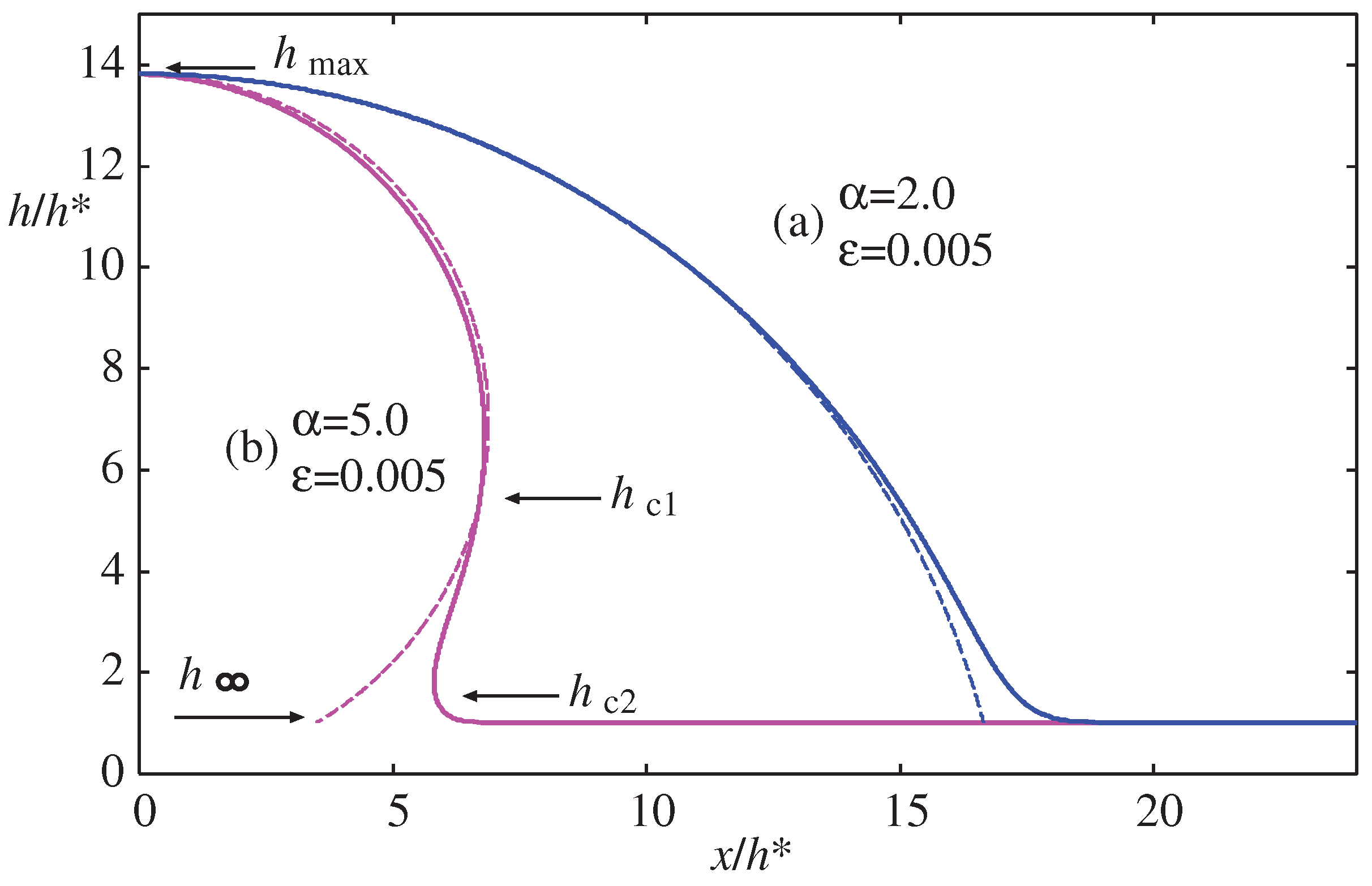
Figure 2.
The disjoining pressure defined by Eq. (34) and the corresponding surface potential calculated by Eq. (4) when and . The thermodynamic potential is defined by Eq. (13) and is plotted for various values of .
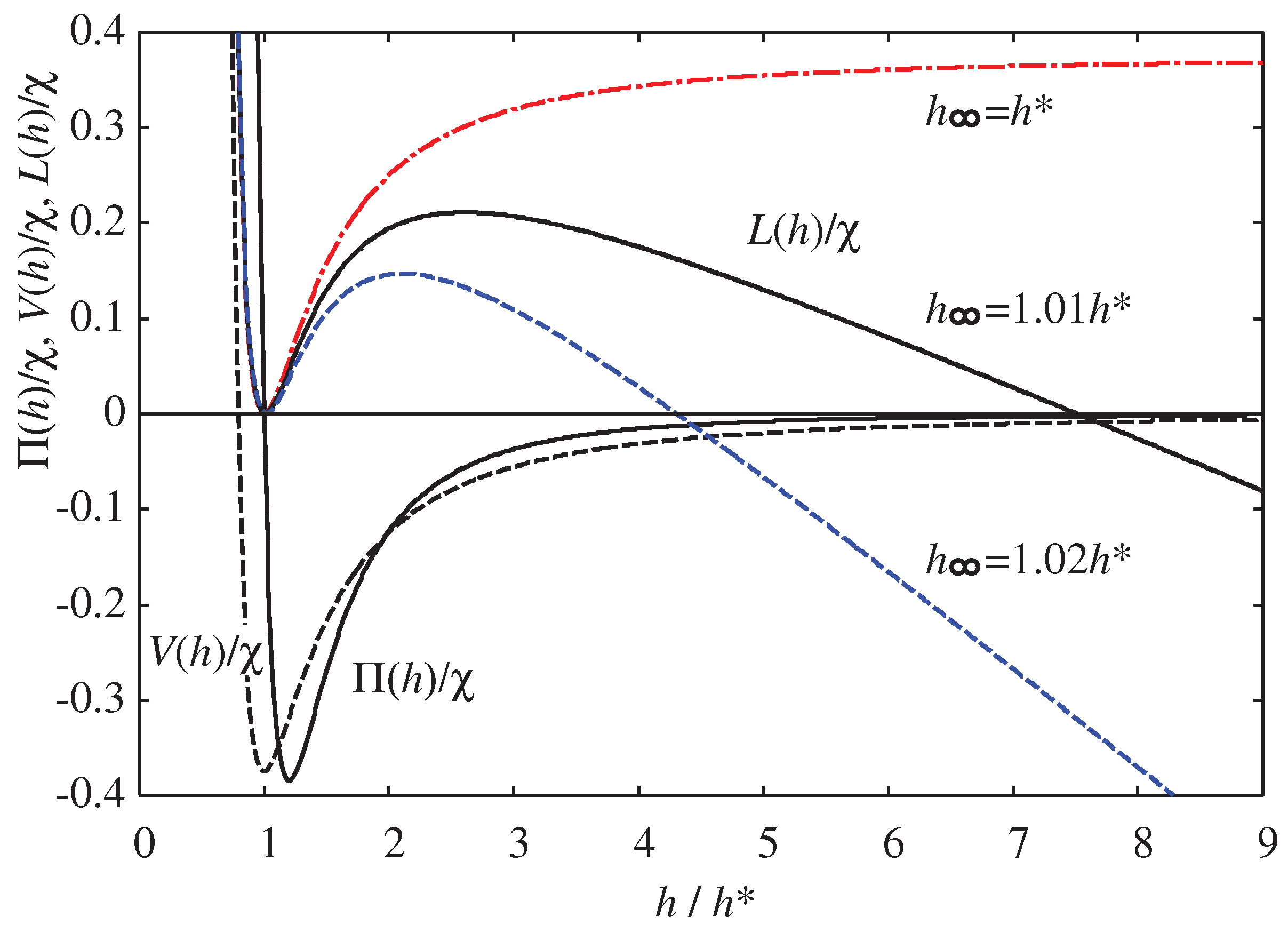
Figure 3.
The absolute value of the excess pressure given by Eq. (35) as a function of the film thickness when and . The absolute pressure reaches its maximum when the film thickness is equal to the value given by Eq. (41), .
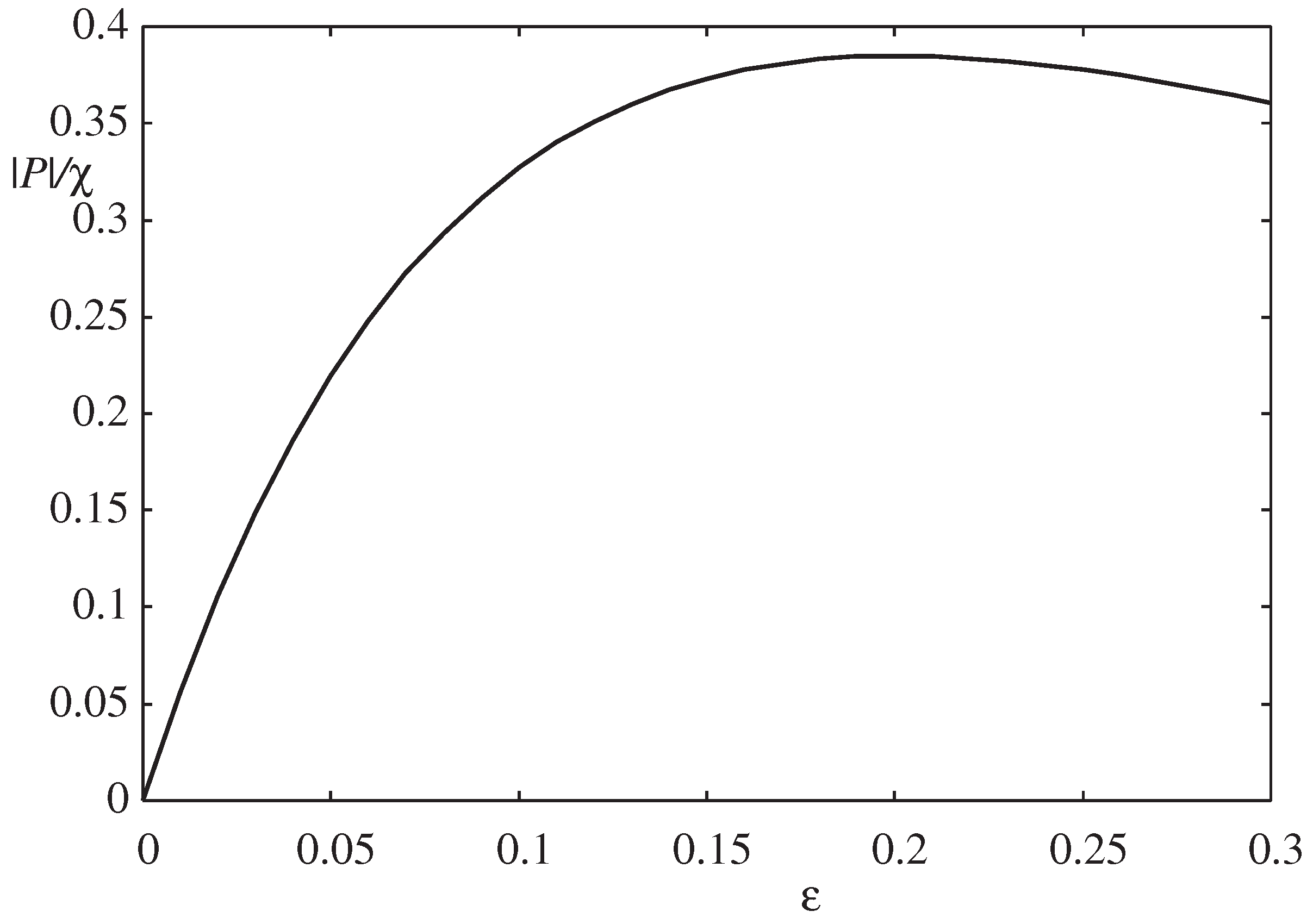
Figure 4.
The functional form of defined by Eq. (38) for various values of () when and . The function shows the maximum when at determined by Eq. (50), which corresponds to the peak of in Figure 2. Its x-intercept determines the maximum height of the droplet by Eq. (42). The graphical determination of two critical heights and from Eq. (46) for a hydrophobic droplet is indicated when and . If , the droplet will be hydrophilic, while if , no droplet can exist according to Eq. (48).
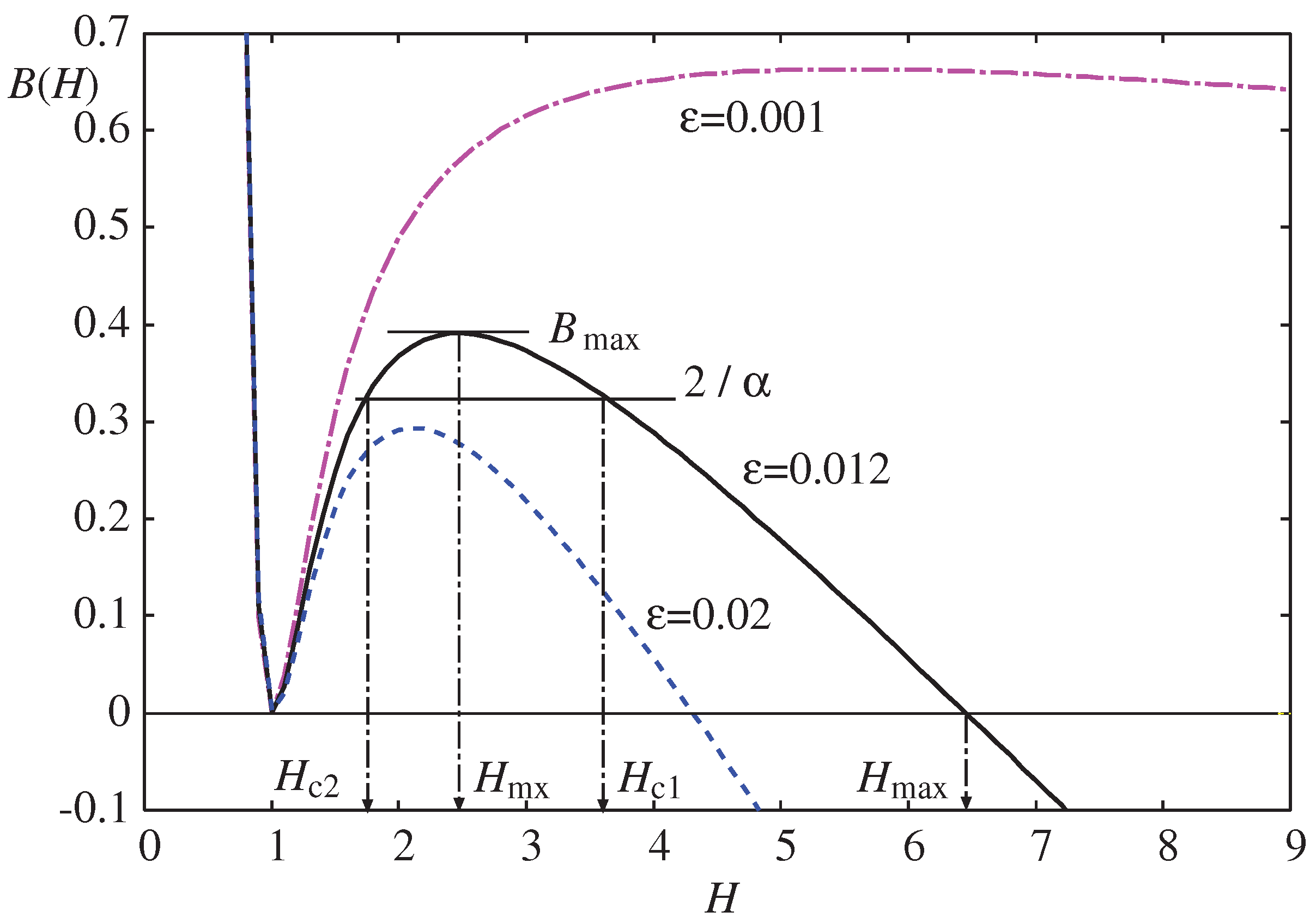
Figure 5.
Two characteristic heights, and , directly calculated numerically from Eqs. (42) and (58) as well as from the approximate analytica formulas in Eqs. (43) and (59) when and . The analytical formulas are only useful near for large droplet (large ).
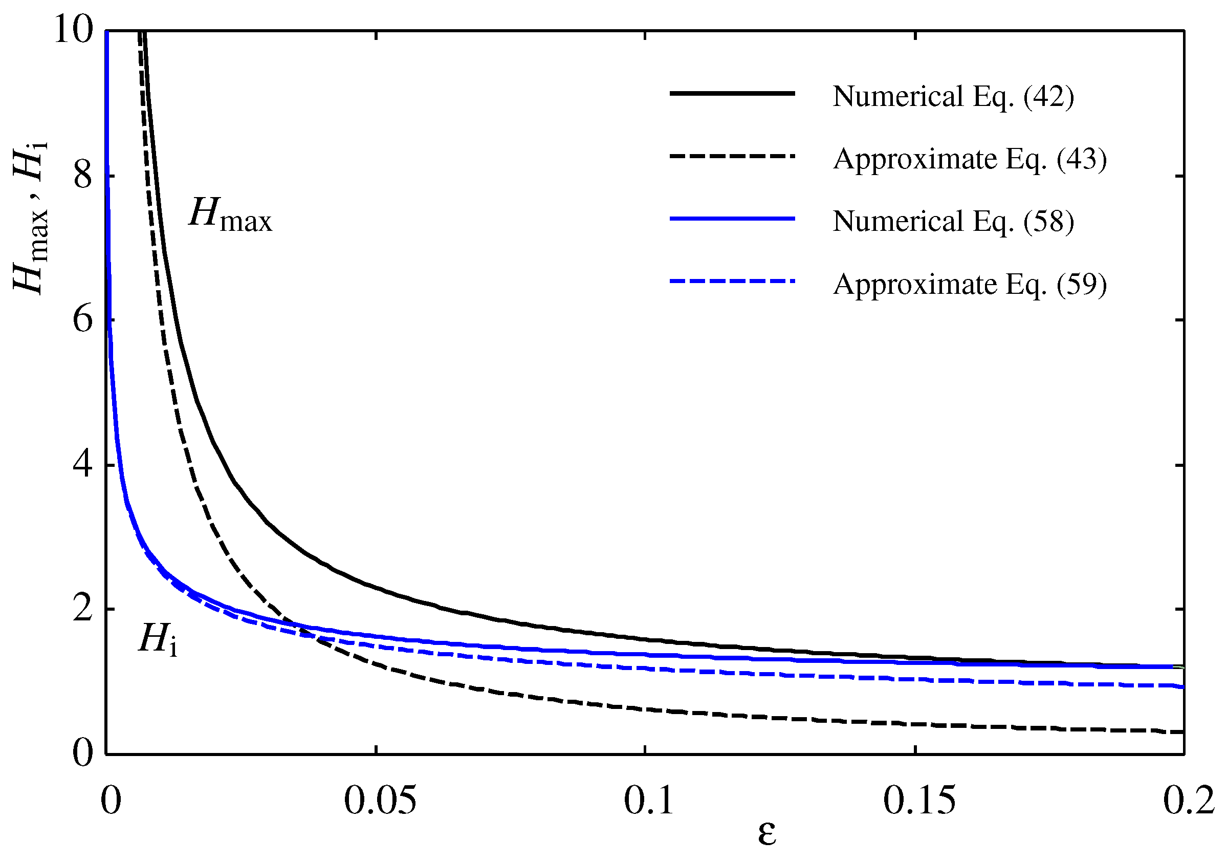
Figure 6.
The no-droplet boundary defined as and the hydrophilic-hydrophobic boundary defined as as a function of film thickness . The macroscopic droplet represents the limit of and as increases the droplet becomes smaller (see Figure 5). The hydrophobic morphology is achieved only when the parameter as given by Eq. (48). Two curves start at and for and in the limit of macroscopic droplets, and increase monotonically. The dashed lines represent the approximation using Eq. (53), which are valid only near . The inset shows an expanded view around and two paths (a) and (b) along which the morphologies in Figure 7a and Figure 7b are calculated. The circular and square symbols indicate the parameter sets used to calculate the morphologies in Figure 7.
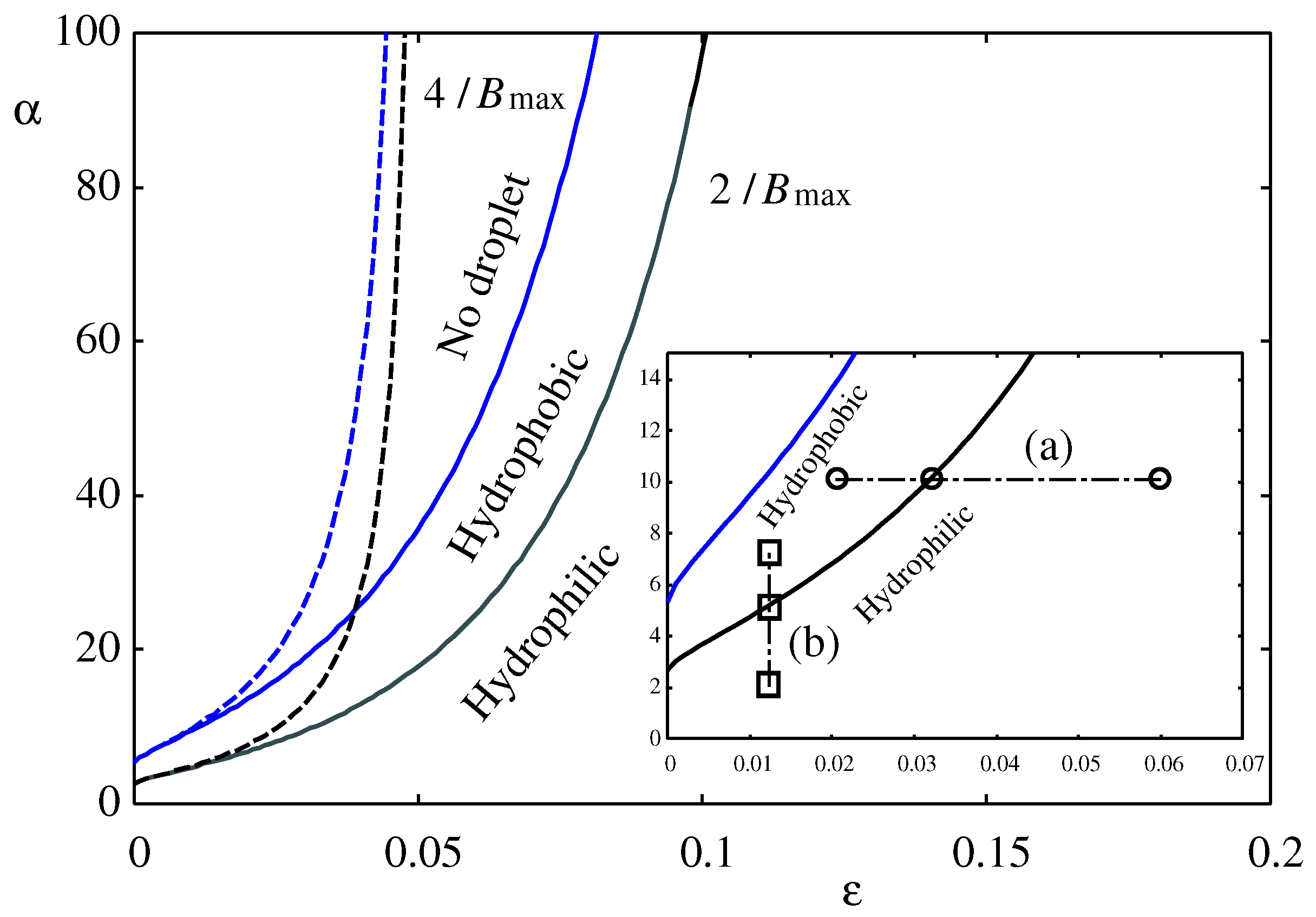
Figure 7.
The morphology of a hydrophilic and a hydrophobic droplet calculated using Eqs. (55) to (56) along the two lines shown in the inset of Figure 6. The vertical axis represents , while the horizontal axis represents . In scenario (a), and . The droplet morphology changes from hydrophobic () to neutral () to hydrophilic (). In scenario (b), and . The droplet morphology changes from hydrophobic () to neutral () to hydrophilic (). The dashed lines represent the cylindrical meniscus with the Laplace radius calculated from Eq. (17). This is not a good approximation for smaller droplets.
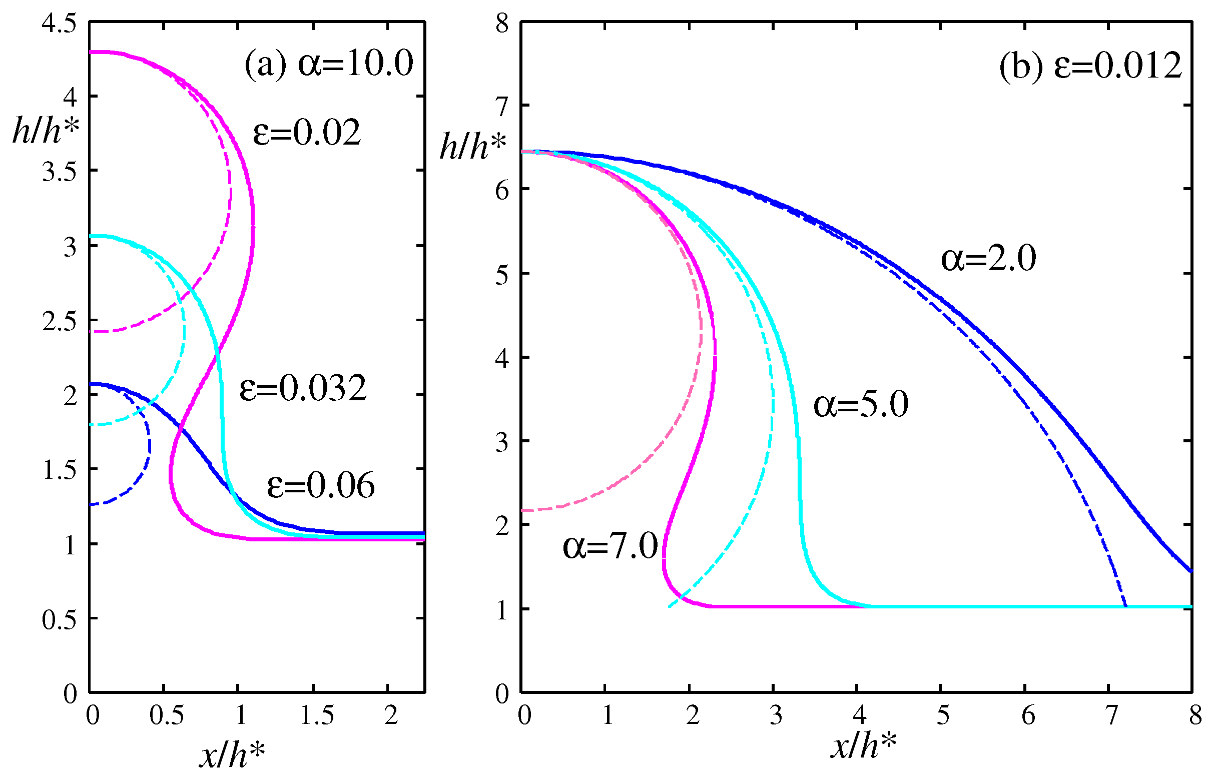
Figure 8.
The analytical effective contact angle obtained by Pekker et al. [21] in Eq. (61) and the macroscopic contact angle from the Derjaguin-Frumkin formula [6,7,14] in Eq. (62) with are compared with the exact numerical results calculated by Eq. (57) as functions of the strength of the surface potential for several values of when and . The contact angles obtained from the exact numerical calculation are generally smaller than and , which are less accurate for hydrophobic droplets with larger . The circles and squares on the exact results indicate the parameter set () that corresponds to those in the paths (a) and (b) in the inset of Figure 6. They are used to calculate the morphologies in Figure 7.
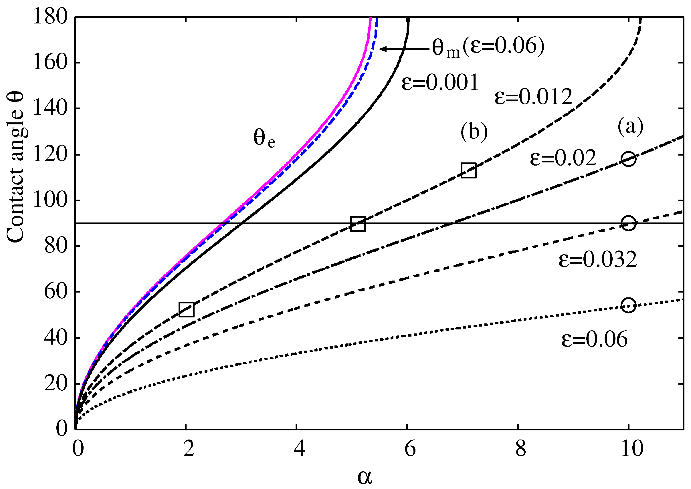
Figure 9.
(a) The cosine of the contact angle, , calculated by Eq. (57) as a function of the inverse of the droplet height, , for several values of the strength of the surface potential . As (macroscopic droplet), where given by Eq. (61). The curves resemble the modified Young’s quation in Eq. (64) with a negative line tension, , if we consider . (b) The hydrophobic-hydrophilic boundary shown in Figure 6 redrawn using instead of as related by Eq 42 (Figure 6). Circular and square symbols are the same as those in Figure 6 and Figure 8.
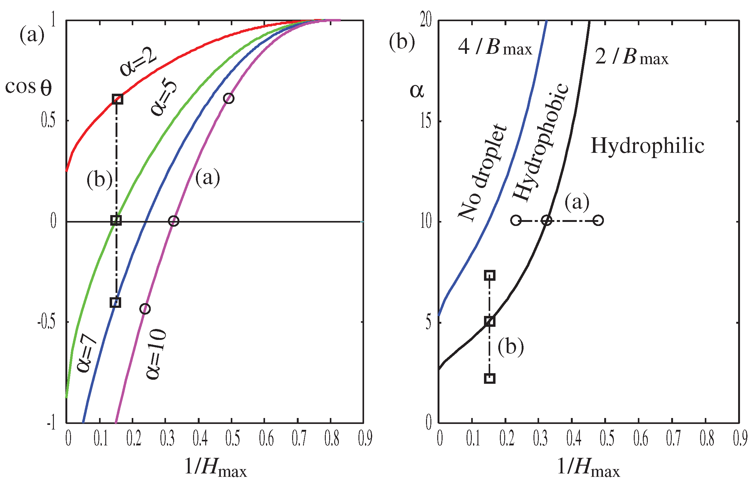

Table 1.
The contact angles numerically calculated from Eq. (57) are compared with from Eqs. (61) and from (62) for the droplets shown in Figure 1 and Figure 7.
| Figure | ||||||
|---|---|---|---|---|---|---|
| 1(a) | 2.0 | 0.0050 | 13.8 | 61.6 | 75.5 | 75.5 |
| 1(b) | 5.0 | 0.0050 | 13.8 | 108.2 | 151.0 | 151.0 |
| 7(a) | 10.0 | 0.060 | 2.07 | 53.7 | - | - |
| 10.0 | 0.032 | 3.07 | 89.4 | - | - | |
| 10.0 | 0.020 | 4.31 | 117.9 | - | - | |
| 7(b) | 2.0 | 0.012 | 6.45 | 52.5 | 75.5 | 75.5 |
| 5.0 | 0.012 | 6.45 | 88.7 | 151.0 | 150.8 | |
| 7.0 | 0.012 | 6.45 | 111.7 | - | - |
Disclaimer/Publisher’s Note: The statements, opinions and data contained in all publications are solely those of the individual author(s) and contributor(s) and not of MDPI and/or the editor(s). MDPI and/or the editor(s) disclaim responsibility for any injury to people or property resulting from any ideas, methods, instructions or products referred to in the content. |
© 2025 by the authors. Licensee MDPI, Basel, Switzerland. This article is an open access article distributed under the terms and conditions of the Creative Commons Attribution (CC BY) license (http://creativecommons.org/licenses/by/4.0/).
Copyright: This open access article is published under a Creative Commons CC BY 4.0 license, which permit the free download, distribution, and reuse, provided that the author and preprint are cited in any reuse.


