
Submitted:
27 November 2025
Posted:
28 November 2025
You are already at the latest version
Abstract
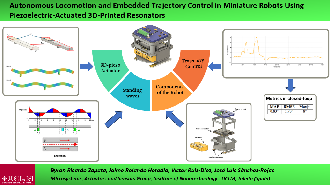
This article presents the design, fabrication, and experimental validation of a centimeter-scale autonomous robot that achieves bidirectional locomotion and trajectory control through 3D-printed resonators actuated by piezoelectricity and integrated with miniature legs. Building on previous works that employed piezoelectric bimorphs, the proposed system replaces them with custom-designed 3D-printed resonant plates that exploit the excitation of standing waves (SW) to generate motion. Each resonator is equipped with strategically positioned passive legs that convert vibratory energy into effective thrust, enabling both linear and rotational movement. A differential drive configuration, implemented through two independently actuated resonators, allows precise guidance and the execution of complex trajectories. The robot integrates onboard control electronics consisting of a microcontroller and inertial sensors, which enable closed-loop trajectory correction via a PD controller and allow autonomous navigation. The experimental results demonstrate high-precision motion control, achieving linear displacement speeds of 8.87 mm/s and a maximum angular velocity of 37.88°/s, while maintaining low power consumption and a compact form factor. Furthermore, the evaluation using the mean absolute error (MAE) yielded a value of 0.83° in trajectory tracking. This work advances the field of robotics and automatic control at the insect scale by integrating efficient piezoelectric actuation, additive manufacturing, and embedded sensing into a single autonomous platform capable of agile and programmable locomotion.
Keywords:
piezoelectric actuation
; miniature robots
; 3D-printed resonators
; standing waves (SW)
; differential drive locomotion
; embedded control
; PD controller
; inertial sensors (IMU)
; additive manufacturing
; autonomous navigation
1. Introduction
Process automation has been the subject of research and development since the emergence of the first autonomous robots, such as Shakey (developed between 1966 and 1972), up to the present day [1]. Since then, efforts have focused on identifying application areas in which repetitive tasks could be automated. The earliest robots featured simple, large, and robust designs, in stark contrast to certain contemporary developments that, in addition to traditional industrial models, also incorporate bioinspired morphologies [2,3].
Bioinspiration adopts conceptual approaches derived from the behavior of various biological organisms. Among them are snakes, worms, geckos, fish, insects, spiders, dogs, and humans, which have been studied to replicate their mobility and adaptive capabilities. These strategies have enabled application proposals in fields such as industry, household environments, medicine, and space exploration, among others [4].
The growing demand for robots in diverse applications has driven the development of devices designed to optimize parameters such as size, mobility, speed, processing capability, and autonomy. These advances have fostered research on robots with various morphologies and scales, including humanoids, robotic arms, soft robots, microrobots, and miniature systems [5]. The miniaturization of electronic systems, enabled by the evolution of Micro-electromechanical systems (MEMS) has made it possible to integrate sensors and control units into autonomous micro- and millimeter-scale robots. This progress has led to the development of prototypes with dimensions comparable to those of insects, whose low weight, reduced size, and agility make them attractive candidates for operation in environments that are difficult to access for conventional robots or humans. Among the most relevant applications of these systems are fault inspection, micromanipulation, minimally invasive medicine, and infrastructure evaluation [6,7,8].
Nevertheless, miniaturization poses significant challenges, such as identifying actuators capable of generating efficient motion at the microrobotic scale. In this context, several alternatives have been proposed, including electromagnetic micromotors with volumes smaller than 1 cm³ [9], shape memory alloys, magnetostrictive materials, artificial muscles, dielectric elastomers, and piezoelectric ceramics, each offering specific advantages and limitations depending on the application [10,11].
At the macroscale, electromagnetic motors have been the predominant actuators. However, at reduced scales their fabrication becomes complex and their energy efficiency decreases [12]. Among the most promising alternatives are piezoelectric actuators, which exploit the inverse piezoelectric effect and offer advantages such as low cost, feasibility of miniaturization, high resolution, robust control, fast response, compact architecture, and immunity to electromagnetic interference, making them particularly attractive for microrobotic applications [13,14].
Friction-based locomotion using piezoelectric actuators involves generating motion by resonator excitation at appropriate frequencies, which establishes standing-wave (SW) or traveling-wave (TW) modes [15]. This principle was described by Siyuan He in the context of bidirectional ultrasonic motors [16]. Based on these fundamentals, different types of architectures and miniature robots have been developed that employ this mechanism to produce linear or rotational movements. In this context, the study [15] applies piezoelectric patches on a resonant plate with attached legs and comparatively analyzes the locomotion obtained through SW and TW. The experimental results show that locomotion based on TW reached speeds of up to 6 BL/s, while the use of SW achieved speeds of up to 14 BL/s, demonstrating that the SW strategy provides significantly higher performance than the TW. At this stage, the prototype was driven by external signals and did not incorporate a microcontroller for autonomous operation.
In [7], the development of a robot measuring 29 × 17 × 18 mm³ and weighing 7.4 g is presented, capable of generating linear and rotational movements through SW waves on a glass surface. The experimental results were promising, reaching a maximum speed of 70 mm/s and a rotational speed of up to 190 °/s. The system presented a power consumption of 50 mW and a continuous operation time of approximately 6.7 hours. The robot managed to follow pre-programmed trajectories, demonstrating agility and control in navigation within complex environments. The limitations present in this work were the adaptation to different surfaces and the lack of sensors that would allow accurate trajectory tracking.
In the context of pursuing autonomy in miniature robots, the authors in [17] designed a robot that emulates the traveling-wave motion of a snail. The robot has dimensions of 27.5 × 26 × 4 mm³ and a weight of 7.9 g, achieving linear speeds of up to 383 mm/s and rotational speeds of 690°/s. It incorporates a 200 mAh battery, providing an approximate operating time of 14.5 minutes, as well as a wireless real-time image acquisition system to determine its position and orientation during navigation. The experimental results demonstrated excellent controllability and great potential for future applications in complex or hard-to-reach environments. Although the robot includes an integrated camera for navigation, there remains the possibility of incorporating additional microsensors to further expand its range of applications.
The use of sensors in miniature robots is a research topic that remains under active development, as sensors open the possibility of achieving complete autonomy and expanding the range of applications. In [18] PVDF piezoelectric materials were used as actuators, together with a microcontroller and a customized infrared sensor module to track a predetermined trajectory. This robot measures 2 cm in size and weighs 1.12 g. It can move at a speed of 96 mm/s and rotate at 280°/s clockwise and 180°/s counterclockwise. The robot successfully followed a black navigation line at an average speed of 3 mm/s, dynamically adjusting its trajectory through infrared feedback and achieving autonomous trajectory correction control. In the context of miniature robots that employ sensors, Kilobot [19] stands out, a 3.3 centimeter-scale robot that integrates infrared and ambient light sensors, as well as [20], which uses a visible light sensor (AS7341) to communicate with other robots and follow trajectories based on light intensity.
Given the importance of sensors in microrobotics, this work proposes the integration of an IMU sensor into a robot driven by piezoelectric actuators using standing waves, with the aim of achieving precise trajectory control. The present article is structured as follows: the Methodology section describes the design and construction of the robot; the Experimental Tests section focuses on validating its performance; and finally, the Discussion and Conclusions section presents the insights derived from this study.
2. Materials and Methods
The methodology for the development of this work is divided into four main parts, which are illustrated in Figure 1.
- 3D-piezo Actuator block represents the use of miniature motors for generating the robot’s movements, built from 3D-printed plates with a defined geometry and incorporating PZT patches.
- Structure Design block represents the structural and 3D printed plates design of the miniature robot; this structure enables the integration of the control and power elements with the PZT actuators.
- Electronic Components block represents the integration of the control and power circuits for the trajectory control of the robot.
- Trajectory Control block represents the design of the algorithm implemented in the microcontroller for movement generation and control.
2.1. 3D-Piezo Actuator
For the locomotion of the miniature robot, unimorph piezoelectric patches of zirconium and titanium (PZT), manufactured with PIC 255 material [21], were employed. Their main characteristics are described in Table 1.
The PZT patches, with dimensions , , and , are placed on top of two plates (A and B) that are 3D-printed using SLA technology with Form3 printer and Formlabs Rigid 10K resin [23]. The PZT patches are fixed to the plates using Loctite. These plates, represented in Figure 2, have dimensions of , , and , with Plate A containing two legs and Plate B one leg, with dimensions of , and . This design and configuration are based on the referenced study [24].
In contrast to [24], in this work the plates are separated by a distance of . This separation allows for a balance between the structure containing the control and power components and the piezoelectric actuators.
The linear movements of the miniature robot are obtained by generating SW on plates A and B, exploiting the structure’s response in flexural modes. These modes allow the legs to be positioned between a node and an antinode of the wave, so that their placement enables the generation of rectilinear trajectories [24,25]. In the present study, the arrangement of the legs follows the description in [24], employing (50) and (60) modes, with legs measuring 1.1 mm in height and 0.6 mm in diameter (Fig. Figure 2 (b)), the actuator patches (PZT piezoelectrics) and leg length were defined based on previous studies [7,15,24]. This configuration ensures stability and enables the generation of linear forward and backward movements, as well as clockwise and counterclockwise rotations.
In this study, (50) and (60) modes were selected because they exhibit maximum amplitudes near the edges and nodal lines toward the interior. This distribution allows the legs to be positioned at the extremities, away from nodal regions, thereby improving the system’s traction and stability compared to other configurations [24].
Figure 3 (a) and Figure 3 (b) show the finite element modal (FEM) analysis performed in SIMSOLID for Plates A and B, where the deformation patterns and the most suitable regions for leg placement can be observed. The color map represents the normalized displacement magnitude, where 1 indicates the maximum deformation and 0 the minimum. These simulations support the final selection of their positions, prioritizing areas with high modal energy and moderate curvature gradients in order to minimize undesired rotations during floor contact.
An important effect related to the control of the miniature robot is associated with the leg–surface interaction, where the direction of motion is reversed compared to the case in which the legs are not in contact. When the legs are positioned to the right of a SW crest, the robot tends to move to the left, whereas placing them to the left of the crest results in motion toward the right. This principle allows mode alternation to generate displacements in different directions, as illustrated in Figure 4.
The combination of (50) and (60) modes produces rotational movements in the clockwise and counterclockwise directions, respectively, as illustrated in Figure 5.
2.2. Electronic Components
The miniature robot actuated by piezoelectric elements is composed of two 3.7 V Li-Po batteries, a microcontroller for trajectory control, and an power circuit that amplifies the excitation signals applied to the piezoelectric actuators. Figure 6 presents an unmounted and assembled view of the robot.
2.2.1. Microcontroller
The robot’s autonomy relies on the acquisition of motion data from the inertial measurement unit (IMU), the implementation of control algorithms, the generation of PWM signals to drive the actuators, and a low-power consumption strategy that collectively enable controlled movements and the maintenance of a defined trajectory. Consequently, the integration of an embedded microcontroller becomes essential. However, the robot’s compact size and the use of batteries for power supply impose strict constraints on the selection of the control unit. Under these conditions, a compact, low-power commercial board that incorporates inertial sensors and meets the requirements of this work is the Seeed Studio XIAO nRF52840 Sense, which has a compact and lightweight form factor (21 × 17,5 mm; ~3 g). This board integrates the Nordic nRF52840 SoC (ARM Cortex-M4; 16 MHz peripheral clock), 1 MB of flash memory and 256 KB of RAM, 11 GPIO with 11 PWM outputs and 6 ADC channels. In addition, it provides UART, I²C, SPI, SWD, NFC and Bluetooth 5.0 communication interfaces.
One of the fundamental features for this work is the on-board sensing, which includes a 6-axis IMU (triaxial accelerometer and gyroscope) and a PDM microphone, with low-power operation ( 5 µA). These characteristics, such as low weight, compact dimensions, communication protocols, low energy consumption, and integrated sensors, are essential for closed-loop trajectory control and provide a solid foundation for future research and developments [26,27].
2.2.2. Power Circuit
After the microcontroller is selected, the power circuit is designed to increase the excitation voltage of the piezoelectric elements. The microcontroller generates PWM signals at 60 kHz for (50) mode and 95 kHz for (60) mode; these signals have an amplitude of 3.3 V. The voltage supplied by the microcontroller is too low to generate the movements of the miniature robot, which is why the circuit shown in Figure 7, based on [28] and [29], is implemented.
The capacitance of the piezoelectric actuators was determined using the practical RC circuit method described in [30]. For this procedure, an Analog Discovery 2 signal generator and a Siglent SDS1104X-E oscilloscope were used to acquire the necessary signals for the calculation. Based on the obtained results, the capacitance of the piezoelectric actuators was determined to be .
Mathematically, the inductance value () of the LC oscillator is determined using equation 1 together with the capacitance of the piezoelectric PZT actuators.
where:
- : Mode frequency for the piezoelectric actuators.
- : Inductance of the oscillator.
- : Capacitance of PZT piezoelectric actuators.
- n: Value used to achieve the maximum peak-to-peak voltage at .
The determination of the values of n, , and from equation 1 has significant implications for the robot’s motion. Several studies, such as [7] and [28] based on [29] , have demonstrated the importance of determining and its effect on the locomotion of robots based on piezoelectric actuators that generate SW waves. In this study, the selection of the inductor is based on equation 1 and on heuristic methods that allow tuning the circuit to the highest resonant frequency corresponding to (60) mode, achieving a high peak-to-peak voltage (Vpp) with low current consumption. Table 2 presents the frequencies evaluated for the different values of n. Additionally, these values were obtained using commercial inductors and measured with a Siglent SDS1104X-E oscilloscope.
Figure 8 shows the circuit response for each inductor listed in Table 2, excited at a frequency of 95 kHz with a 50% duty cycle. These inductors were selected because they represent the upper and lower operating limits before signal distortion occurs and the current exceeds 600 mA, which is the maximum value supported by the 2N2222A transistor in its SOT-23 package.
To maintain a proper relationship between high voltage levels and low current levels, the commercial inductor of 470 µH was selected. It is worth mentioning that the waveform is linked to the relationship between duty cycle and frequency. This analysis is presented in Figure 9, where the duty cycle is varied from 40% to 75% while maintaining the frequency constant at 95 kHz using the 470 µH inductor.
Based on this analysis, it is observed that duty cycles between 50% and 65% exhibit a similar behavior. However, considering the robot’s displacement and the incorporation of both piezoelectric actuators, better results were achieved when selecting a 65% duty cycle. At this value, the signal shows no appreciable distortion and maintains a stable voltage of approximately 81.2 Vpp with a current of 30 mA, thereby ensuring an adequate excitation of the piezoelectric actuators.
2.3. Energy Consumption in the Batteries
The miniature robot uses two 401010 Li-Po batteries connected in series in order to provide a voltage of 7.4 V. This voltage powers the LC resonator circuit (Figure 7) and an AMS1117 voltage regulator, which steps the voltage down to 3.3 V to power the microcontroller. The electronic schematic of the miniature robot is shown in Figure 10.
The key specifications of these batteries are presented in Table 3.
To determine the operating time of the miniature robot, the maximum current consumption of the microcontroller and the power circuit are summed, and equation 2 is applied, following [32].
Where:
- t: Battery duration.
- C: Battery capacity.
- : Battery efficiency.
- : Average current considering the consumption of the microcontroller with the IMU sensor, Bluetooth module, and status LEDs turned on, along with the power circuit operating at 60 kHz.
2.4. Design of the Miniature Robot Structure
The structural design of the robot was conceived in a compact and lightweight manner, so that it could incorporate and support the mass of the electronic components listed in Table 4. It is worth noting that the weights presented correspond to experimental measurements of the physical components.
The miniature robot structure consists of four stages, as shown in Figure 11:
- Lower stage (1): Designed to house the batteries.
- Intermediate stage (2): Designed to place and support the microcontroller.
- Upper stage (3): Allows the placement of the oscillator circuit.
- Support pillars (4): Connect plates A and B with the robot structure for motion generation.
The structure was manufactured by 3D printing in Clear resin from Formlabs using SLA printer [33]. The final dimensions of the structure were: length of 26 mm, width of 26.95 mm, and height of 23.8 mm, with a total mass of 1.8 g (Figure 12 (a)). The support pillars have a cylindrical geometry, with a height of 2.8 mm and a diameter of 0.6 mm. To minimize vibration disturbances, the pillars are positioned at the midpoint between the first two nodal points of (50) and (60) modes. This selected position is located 1.25 mm from the beginning and end of plates A and B, respectively, as shown in Figure 12 (b).
To validate the design, a structural analysis was performed with SimSolid, considering the mechanical properties of the resin and the point loads from Table 3. The static analysis evaluated the total displacements and the equivalent Von Mises stresses.
The simulation results showed a maximum displacement of at the point shown in Figure 13 (a), this value is negligible with respect to the dimensions of the structure. The Von Mises stresses are shown in Figure 13 (b), these stresses are between and , which represents 0.234% of the material capacity. Therefore, the designed structure is capable of safely supporting all the considered components.
The integration of the miniature robot’s components is presented in Figure 14. In the side view (Figure 14 (a)), the oscillator circuit is mounted on the top of the structure and secured at its corners with a cyanoacrylate-based adhesive (Loctite). The top view (Figure 14 (b)) shows the junction of the pillars with plates A and B; this joint was made with the same adhesive to ensure a rigid, stable connection.
The connection between the microcontroller, the resonance plate and the piezoelectrics is made using enameled copper wires of 10 µm in diameter. The assembled prototype maintains the dimensions established in the previous design (26 × 26.95 × 24.2 mm) and a total weight of 9 g.
The compact distribution of the components ensures the stability of the robot and allows efficient integration of the electrical and mechanical systems.
2.5. Trajectory Control
To control the trajectory of the miniature robot, a closed-loop control system is implemented with a zero reference . The system integrates an IMU sensor to estimate the robot’s rotation angle and direction , a control signal that modulates the frequency applied to the piezoelectric actuators , and a control algorithm designed to minimize the tracking error. Figure 15 presents the block diagram used for the robot control system.
2.5.1. IMU Sensor
The microcontroller integrates an LSM6DS3 inertial sensor with six degrees of freedom (triaxial gyroscope and triaxial accelerometer, 16-bit). In the selected configuration, the gyroscope operates at with a sensitivity of , and the accelerometer at with a sensitivity of ; these ranges were chosen to prevent saturation and to enable precise capture of rapid motion variations and large-magnitude accelerations during frequency changes in the miniature robot’s movement [34]. The axis reference used throughout the processing is defined with respect to the board: the X axis points toward the USB connector, the Y axis points to the left side (with the USB on the right), and the Z axis is perpendicular to the PCB, pointing outward. The components measure linear acceleration along these directions, and represent angular velocity about each axis, with positive sign defined by the right-hand rule.
2.5.2. Kalman Filter
The data acquired from both sensors are processed using a Kalman filter, which effectively mitigates oscillations arising from the device’s intrinsic disturbances as well as vibrations induced by the piezoelectric actuators. For the application of the Kalman filter, the prediction and update equations presented in 3 and 5 were applied [35].
The prediction step is defined in equation 3.
where corresponds to the a priori estimated state, the a posteriori state, the a priori error covariance, the a posteriori error covariance, and Q the process noise covariance constant. In this work, the values and were used to simplify the expressions, as shown in 4.
The update step is presented in equation 5:
where represents the Kalman gain, R the measurement noise covariance, the current sensor measurement, and the updated error covariance. In this case, the value was assigned for the reduction in expression 6.
The parameters presented in Table 5 were selected to achieve a balance between responsiveness and sensor noise attenuation. With these values, the intrinsic noise of the system and the vibrations from the piezoelectric actuators are effectively reduced. Figure 16 shows the significant reduction of gyroscope perturbations in the Z-axis.
In this study, only the Z-axis rotation values are considered due to the position of the microcontroller and the direction that needs to be corrected for position control.
2.5.3. Gyroscope Calibration and Angle Estimation
As shown in Figure 16, when the miniature robot is at rest, it exhibits random noise and signal drift, which introduce a systematic bias in the measurement of angular velocity. Since the angular velocity should ideally be zero at rest, the bias error is determined using equation 7 [36]:
Where:
- N: total number of acquired samples.
- : gyroscope signal acquired from instant to N.
The determined bias value represents the average displacement of the acquired signals. To ensure that the sensor values are centered around zero during the resting state, the corrected measurement is applied using equation 8:
Where represents the corrected angular velocity measurement after eliminating the average noise. In this work, gyroscope calibration was performed by keeping the miniature robot at rest from s to s, with a sampling period of 2 ms, resulting in approximately 1000 samples.
The corrected measurement helps reduce the accumulation of errors when transforming angular velocity into angular position . For this purpose, the integral of the angular velocity is applied, as shown in equation 9:
Since the continuous integral in equation 9 cannot be directly implemented in the microcontroller, a discrete approximation is employed to integrate the corrected angular velocity with a sampling period of ms, as expressed in equation 10:
Where represents the angular position in radians.
2.5.4. PD Control
The motion of the miniature robot is regulated by a Proportional Derivative (PD) controller, which adjusts the frequency applied to the piezoelectric actuators to maintain a predefined path. This application allows correcting the angular position based on the feedback provided by the gyroscope.
The regulation is based on the hysteresis curve shown in Figure 17.
The midpoint allows both actuators, A and B, to remain in (50) mode at a frequency of 60 kHz, while the positive phase of the hysteresis curve allows actuator B to switch to (60) mode, with a frequency of 95 kHz, and actuator A to remain in (50) mode to generate a counterclockwise rotation of the robot. The negative phase of the hysteresis allows a clockwise rotation, setting actuator A to (60) mode and actuator B to (50) mode. The base frequency of 60 kHz is selected on the ascending slope of the (50) mode resonance to maximize amplitude modulation, while 95 kHz is used to fully excite the (60) mode.
The general function used for actuators A and B is presented in equation 11:
where represents the frequency value sent to the PWM of the respective actuators and is the value of the PD controller output.
To assign the frequencies to the respective actuators, equation 12 is used:
To limit the frequencies sent to each actuator, a saturator is used, expressed as equation 13:
The output of the controller in continuous time is defined as:
The backward difference approximation of equation 14 for the discrete PD controller is defined as:
where:
- : Proportional gain.
- : Derivative gain.
- : Error between the reference and the gyroscope measurement at the current instant.
- : Error between the reference and the gyroscope measurement at the previous instant.
- : Sampling period.
The tuning of the and values was carried out experimentally through a heuristic procedure, with the aim of achieving a balance between response speed and system stability. The proportional gain was increased up to a value of 700, which allowed a fast response to trajectory changes. Subsequently, the derivative gain was set to 80 in order to reduce overshoot and attenuate system oscillations. The parameter adjustment employed in this work proved to be more effective compared to the model identification of the robot obtained by software. It should be noted that software-based identification presents limitations due to gyroscope noise and the nonlinear dynamics of the robot, which leads to an approximation that is not fully representative of the real model. In contrast, experimental tuning allowed establishing and values that provided satisfactory performance in terms of speed and stability under real operating conditions.
Substituting the values of and , with a sampling time of , into equation 16, we obtain:
3. Results
The experimental evaluation of the miniature robot was structured into four main tests:
- Conductance test of plates A and B, aimed at validating the electrical response of the piezoelectric resonators when excited in (50) and (60) modes.
- Linear displacement velocity test, performed to determine the average forward speed of locomotion.
- Angular velocity test, designed to evaluate clockwise and counterclockwise rotational movements.
-
Trajectory error tests, carried out under two conditions:
- (a)
- without trajectory control, and
- (b)
- with proportional–derivative (PD) control for path correction.
These tests provide the basis for determining the generation of movement, linear speed of locomotion, maneuverability for rotation, and trajectory correction of the proposed robot. The detailed results of each test are presented in the following subsections.
3.1. Conductance Test of Plates A and B
The objective of this test was to validate the electrical response of the piezoelectric actuators coupled to plates A and B. For this purpose, a series RC circuit was implemented, in which a resistor was connected in series with each of the piezoelectric actuators. Using an Analog Discovery 2 board, a sinusoidal signal in the range of 40 to 100 kHz, with an amplitude of 500 mV, was applied.
The frequency response obtained is shown in Figure 18, where resonance peaks corresponding to (50) and (60) modes can be observed.
The quantitative results of the test are summarized in Table 6, where it can be observed that for (50) mode, the resonant frequencies are located at 62.37 kHz for plate A and 60.67 kHz for plate B, with conductance values of 43.4 and 40.2 S, respectively. For (60) mode, the peaks appear at 91.16 kHz and 92.01 kHz for plates A and B, respectively, reaching conductances of 67.8 and 115.7 S.
Based on the obtained results, the characteristic frequencies of each plate can be identified and their conductance quantified. In comparative terms, it can be seen that plate B exhibits higher conductance in (60) mode compared to plate A, which suggests better electrical coupling in this mode. These results provide a basis for the evaluation of subsequent dynamic tests.
3.2. Linear Displacement and Angular Velocity Test
This test involves the study of linear displacement and both clockwise and counterclockwise rotation of the uncontrolled robot. As an initial test to determine linear displacement, the travel time of the robot along a 20 mm path was measured. The experiment was conducted on a mm glass plate printed with a 5 mm grid; start and end marks were placed 20 mm apart. Each trial was executed using a timer that triggered the robot’s excitation at the start mark and stopped it at the end mark, recording the elapsed time. The robot was always positioned at the same initial point and driven at 60 kHz with a 65% duty cycle on plates A and B. Before each trial, the battery was verified to be fully charged (7.4 V). A total of n = 10 consecutive trials were conducted, and the time required for each repetition was recorded, yielding a mean time of . Based on this value, the displacement velocity was calculated using the expression , considering a fixed distance of , which resulted in an average velocity of . The boxplot of the displacement test is shown in light blue in Figure 19, where low variability between trials can be observed, with a standard deviation of 0.086 s and no outliers detected.
To determine the rotational speed in both clockwise and counterclockwise directions, tests were conducted on the same surface used for the linear displacement test, setting a reference angle of . For clockwise rotation, plates A and B were excited at frequencies of 60 kHz and 91 kHz, respectively, applying a duty cycle of 65% in both cases. In the counterclockwise test, the actuators were excited at frequencies of 92 kHz and 60 kHz, maintaining the same duty cycle. The average time recorded in the rotation tests was for clockwise and for counterclockwise motion. Based on these values, and applying the expression with a fixed angle of , the corresponding average angular velocities were calculated as and , respectively.
Figure 19 presents the boxplots corresponding to the rotation times. From these results, the standard deviation was calculated as for clockwise rotation and for counterclockwise rotation. These values indicate moderate variability in the trials, slightly higher in the clockwise direction.
The relative variation in the recorded times was low, indicating high repeatability and consistency throughout the experiment. Overall, the results show that, despite the small differences between the two rotation directions, the robot maintains stable and repeatable performance, confirming the system’s capability to generate consistent and reproducible movements.
The experimental setup and robot locomotion can be observed in the supplementary video (Video S1).
3.3. Trajectory Error Tests
The open-loop trajectory (without trajectory control) was evaluated by exciting actuators A and B at frequencies of 61 kHz and 63 kHz and a duty cycle of 65% respectively. To analyze the movement, a trajectory was defined on the horizontal axis , and the robot position was measured using a fixed camera placed parallel to the surface of the squared glass. Figure 20 (Robot displacement without control) shows the measured linear trajectory and the desired reference over 20 s. In this first open-loop test, the trajectory error was calculated using , representing the linear deviation in millimeters. At the end of the linear displacement test ( s), the robot accumulated a linear error of 58 mm relative to the reference.
A second open-loop test was performed to evaluate the robot’s rotational drift using the gyroscopic sensor. Figure 20 (Z Angle vs Time) shows the accumulated angular deviation of the robot with respect to the initial reference . At the end of the test (), the angular error reached approximately .
The angular deviations in the trajectory were evaluated using the metrics: mean absolute error (MAE), root mean square error (RMSE), and the maximum absolute error ().
The values in Table 7 show considerable deviations with respect to the reference, confirming the need to implement a closed-loop controller.
For the trajectory control in closed-loop, a PD controller designed in Subsection 2.5.4 was applied. A reference was set on the horizontal axis , and the robot position was measured using a fixed camera placed parallel to the squared glass surface. Figure 21 (Robot displacement with trajectory control) shows the measured trajectory and the reference during a 20-second interval after applying the controller, in this graph, an average error of approximately 4 mm is observed between the reference trajectory and the robot position.
To validate the controller response, the gyroscope output was analyzed again, setting a reference of and recording the robot response for 12 seconds. Figure 21 (Z Angle vs Time) presents the angular response obtained.
Table 8 summarizes the mean of ten trials conducted under equivalent experimental conditions on the same surface.
The values show a significant reduction in trajectory tracking error through the application of the PD controller, decreasing both the mean error and the maximum absolute error compared to the open-loop case.
In Figure 22, the excitation frequency of the control signal sent to piezoelectric actuators A and B is presented as a function of time.
4. Discussion
A key finding is the experimental validation of high-precision autonomous navigation. The system achieved a linear speed of 8.87 mm/s in straight-line motion and angular velocities of 37.87°/s and 28.30°/s in clockwise and counterclockwise rotation, respectively, maintaining a straight trajectory with a MAE of only 0.83°. This emphasis on closed-loop trajectory-tracking accuracy distinguishes our robot from previous works that prioritized open-loop speed. For instance, studies such as [7] reported significantly higher linear velocities (70 mm/s) using similar standing-wave (SW) actuation in 7.4 g robots, yet lacked the onboard sensing and closed-loop correction achieved in this prototype. Therefore, our work contributes to the advancement of control techniques at the miniature scale.
The simplified excitation circuit, previously described in the literature [28,29], was empirically validated in this study, confirming its suitability for generating high excitation voltages up to 81.2 Vpp at 100 kHz with low currents of about 30 mA. The use of two 7.4 V, 30 mAh batteries optimized the balance between speed, force, and endurance. Compared with Flyback circuits reported in other studies [37,38,39,40], the proposed design offers advantages in weight, size, and power consumption parameters that are critical for miniaturized robotic platforms. This electronic optimization represents a tangible step toward the full integration of autonomous systems at reduced scales.
The successful implementation of the Seeed Studio nRF52840 XIAO microcontroller was essential, validating the feasibility of integrated control in miniature robots and enabling wireless communication for real-time monitoring. The effective integration of piezoelectric actuators, compact electronics, and embedded autonomous control consolidates an efficient and versatile miniaturized platform focused on small-scale control research. A crucial factor in the robot’s autonomy was battery performance: the operating current consumption (estimated between 50 mA and 60 mA) depleted the 30 mAh battery in approximately 24 minutes. This consumption is mainly associated with the control, power, and wireless communication modules used for trajectory management. Such limited endurance remains a primary constraint of the current platform, in marked contrast to the multi-hour operation reported in [7], and should be a major target for future optimization.
Finally, the results open promising research directions toward the implementation of integrated machine-learning techniques (TinyML). Having established a platform capable of stable and programmable motion control, the next logical step is to explore real-time decision-making and advanced perception systems, positioning the developed platform as a solid foundation for the advancement of intelligent and autonomous microrobotics.
5. Conclusions
In this work, a miniature robot with a total weight of 9 g and dimensions of 26 × 26.95 × 24.2 mm was developed and experimentally validated. The robot was propelled by 3D-printed resonators equipped with PZT piezoelectric patches, enabling both linear and rotational motion. The prototype achieved linear speeds of 8.87 mm/s and angular velocities of 37.88°/s and 28.31°/s in the clockwise and counterclockwise directions, respectively. These displacements were obtained through the excitation of SW waves, generated by a compact and low-power microcontroller capable of producing pulse-type signals at frequencies between 60 and 95 kHz with a duty cycle of 65%. The signals were amplified by a resonant LC circuit powered by two 3.7 V – 30 mAh batteries.
The design of the LC circuit was based on previous studies and an experimental analysis aimed at determining the optimal Vpp values and operating frequencies that prevent waveform distortion and excessive current peaks. As a result, an inductor of 470 µH was selected with duty cycles between 50% and 65%, allowing operation within the 60–95 kHz range, where the flexural (50) and (60) modes are excited to produce the robot’s motion.
Finally, using the Seeed Studio XIAO nRF52840 Sense microcontroller, chosen for its compact size, low power consumption, and integrated IMU sensor, a proportional–derivative controller was implemented to maintain the robot’s straight-line trajectory. Experimental tests reported a MAE of 0.83°, demonstrating the feasibility of embedded control on a small scale and its potential for future applications of multimodal locomotion control techniques, improved estimation algorithms, and the transition toward fully autonomous microrobotic systems.
Supplementary Materials
The following are available online at Preprints.org
- Video S1—Experimental setup and robot locomotion (linear and rotational). Locomotion of the miniature robot under standing-wave (SW) excitation. Linear displacements and clockwise/counterclockwise rotations are observed, with close-ups of the resonator–leg contact and of the surface used for motion tracking. Direct link: https://drive.google.com/file/d/1uxGeuC2jyAQUHhNXmyPUsnJr-TAFGblO/view?usp=sharing
- Video S2—Open-loop linear displacement at 61 kHz and 63 kHz (65% duty cycle). Open-loop trials showing the frequency-dependent response. Frequencies of 61 kHz and 63 kHz (PWM at 65%) are applied to actuators A and B, evidencing forward motion. Direct link: https://drive.google.com/file/d/1neRBwMGSnG6WycQ3dUlyWCIgMFHX4H-w/view?usp=drive_link
- Video S3—Closed-loop trajectory control with an embedded PD controller. Demonstration of on-board sensing and control: yaw feedback via IMU, filtered (Kalman) estimation, and a proportional–derivative (PD) controller that regulates the excitation frequency to maintain a straight path. The video shows representative linear and angular responses under closed-loop operation. Direct link: https://drive.google.com/file/d/1C5pN0fRFXgL4qbrd8cdHi9qoc2mZjmBE/view?usp=sharing
Author Contributions
Conceptualization, V.R.-D., and J.L.S.-R.; software B.Z.C. and J.H.V.; investigation, B.Z.C. and J.H.V.; data curation, B.Z.C. and J.H.V.; writing-original draft preparation, B.Z.C. and J.H.V.; writing-review and editing, V.R.-D., and J.L.S.-R.; project administration, V.R.-D., and J.L.S.-R.; funding acquisition, V.R.-D., and J.L.S.-R. All authors have read and agreed to the published version of the manuscript.
Funding
This work was supported by the Universidad de Castilla-La Mancha, Spain, through MCIN/AEI and FEDER "ERDF A way of making Europe" under Grant PID2023-146163OB-I00 and Universidad Politécnica Salesiana, Quito-Ecuador.
Institutional Review Board Statement
Not applicable.
Informed Consent Statement
Not applicable.
Data Availability Statement
The datasets presented in this article are not readily available because the data are part of an ongoing study and due to technical/ time limitations. Requests to access the datasets should be directed to bzapata@ups.edu.ec.
Conflicts of Interest
The authors declare no conflicts of interest. The funders had no role in the design of the study; in the collection, analyses, or interpretation of data; in the writing of the manuscript, or in the decision to publish the results.
References
- Siciliano, B.; Khatib, O., Eds. Springer Handbook of Robotics, 2 ed.; Springer: Cham, Switzerland, 2016. [CrossRef]
- Pfeifer, R.; Lungarella, M.; Iida, F. The Challenges Ahead for Bio-Inspired ’Soft’ Robotics. In Proceedings of the Transactions of the Royal Society B, 2012, Vol. 367, pp. 178–200. [CrossRef]
- Hammond, M.; et al.. Bioinspired Soft Robotics: State of the Art, Challenges, and Opportunities. arXiv preprint arXiv:2312.12312 2023.
- Zhang, Y.; Li, J.; Chen, X.; Wang, H. Bioinspired Sensors and Applications in Intelligent Robots: A Review. Robotics and Artificial Intelligence 2023, 10, 88–104. [CrossRef]
- Bandari, V.K.; Eom, S.H.; Park, H.; Lee, S.W.; Jeong, U. System-Engineered Miniaturized Robots: From Structure to Intelligence. Advanced Intelligent Systems 2021, 3, 2000284. [CrossRef]
- Li, Z.; Li, C.; Dong, L.; Zhao, J. A Review of Microrobot’s System: Towards System Integration for Autonomous Actuation In Vivo. Micromachines 2021, 12, 1249. [CrossRef]
- Ramírez-Palma, M.R.; Robles-Cuenca, D.; Ruiz-Díez, V.; Hernando-García, J.; Sánchez-Rojas, J.L. Vibration Propulsion in Untethered Insect-Scale Robots. Robotics 2024, 13, 135. [CrossRef]
- collective, A. Locomotion for Insect-Scale Robots With Bionic Strategies: A Review. Journal of Field Robotics 2024. [CrossRef]
- Kim, H.J.; Kim, S.M.; Kim, H.T.; Yi, B.J. An Omnidirectional Mobile Millimeters Size Micro-Robot. International Journal of Advanced Robotic Systems 2008, 5, 41–46. [CrossRef]
- Mittal, V.; Singh, R. A Review of Bio-Inspired Actuators and Their Potential for Autonomous Systems. Actuators 2025, 14, 303. [CrossRef]
- Zhu, B.; Li, C.; Wu, Z.; Li, Y. A double-beam piezoelectric robot based on the principle of two-mode excitation. Sensors and Actuators A: Physical 2024, 369, 115154. [CrossRef]
- Cheng, J.; Xue, N.; Qiu, B.; Qin, B.; Zhao, Q.; Fang, G.; Yao, Z.; Zhou, W.; Sun, X. Recent Design and Application Advances in Micro-Electro-Mechanical System (MEMS) Electromagnetic Actuators. Micromachines 2025, 16, 670. [CrossRef]
- Hernando-García, J.; García-Caraballo, J.L.; Ruiz-Díez, V.; Sánchez-Rojas, J.L. Motion of a Legged Bidirectional Miniature Piezoelectric Robot Based on Traveling Wave Generation. Micromachines 2020, 11, 321. [CrossRef]
- Wang, Y.; Zhang, L.; Zhao, H.; Li, Y.; Zhao, X. A spatial 3-DOF piezoelectric robot and its speed-up trajectory based on improved stick-slip principle. Mechanical Systems and Signal Processing 2021, 150, 107247. [CrossRef]
- Ruiz-Díez, V.; Hernando-García, J.; Toledo, J.; Ababneh, A.; Seidel, H.; Sánchez-Rojas, J.L. Comparative Study of Traveling and Standing Wave-Based Locomotion of Legged Bidirectional Miniature Piezoelectric Robots. Actuators 2021, 10, 136. [CrossRef]
- He, S.; Chen, W.; Tao, X.; Chen, Z. Standing Wave Bi-directional Linearly Moving Ultrasonic Motor. IEEE Transactions on Ultrasonics, Ferroelectrics, and Frequency Control 1998, 45, 1133–1139. [CrossRef]
- Wang, W.; Li, J.; Zhang, S.; Deng, J.; Chen, W.; Liu, Y. A Snail-Inspired Traveling-Wave-Driven Miniature Piezoelectric Robot. Applied Physics Letters 2023, 122, 063701. [CrossRef]
- Wu, Y.; Cao, L.; Lu, G.; Wang, P.; Ran, L.; Peng, B. Untethered Soft Microrobot Driven by a Single Actuator for Agile Navigations. Nature Communications 2025, 16, 61810. [CrossRef]
- Rubenstein, M.; Ahler, C.; Nagpal, R. Kilobot: A Low Cost Scalable Robot System for Collective Behaviors. In Proceedings of the Proceedings of the 2012 IEEE International Conference on Robotics and Automation (ICRA), Saint Paul, Minnesota, USA, May 2012; pp. 3293–3298. [CrossRef]
- Zhu, R.; Zhang, Y.; Wang, H. Miniature Mobile Robot Using Only One Tilted Vibration Motor. Micromachines 2021, 12, 1103. [CrossRef]
- Ceramic, P. PI Ceramic Material Data. Datasheet, 2025. Accessed: 20 November 2025.
- PI Ceramic. Piezo Actuator Materials Tutorial. Physik Instrumente (PI) GmbH & Co. KG, Lederhose, Germany, 2004. Technical tutorial on piezoelectric actuator materials.
- Formlabs Inc. Rigid 10K Resin—Technical Data Sheet (TDS). https://formlabs-media.formlabs.com/datasheets/2001479-TDS-ENUS-0.pdf, 2022. Rev. 03; drafted on 2020-10-07.
- Ruiz-Díez, V.; García-Caraballo, J.L.; Hernando-García, J.; Sánchez-Rojas, J.L. 3D-Printed Miniature Robots with Piezoelectric Actuation for Locomotion and Steering Maneuverability Applications. Actuators 2021, 10, 335. [CrossRef]
- Ruiz-Díez, V.; Hernando-García, J.; Toledo, J.; Ababneh, A.; Seidel, H.; Sánchez-Rojas, J.L. Piezoelectric MEMS Linear Motor for Nanopositioning Applications. Actuators 2021, 10, 36. [CrossRef]
- Seeed Studio. Seeed Studio XIAO nRF52840 Sense Product Specification v1.5. Seeed Studio, Shenzhen, China, 2024. Accessed: 10 October 2025.
- Rovai, M.J. XIAO: Big Power, Small Board; GitHub eBook, 2023. Accessed: 10 October 2025.
- Robles-Cuenca, D.; Ramírez-Palma, M.R.; Ruiz-Díez, V.; Hernando-García, J.; Sánchez-Rojas, J.L. Miniature Autonomous Robot Based on Legged In-Plane Piezoelectric Resonators with Onboard Power and Control. Micromachines 2022, 13, 1815. [CrossRef]
- EDN. Increase Piezoelectric Transducer Acoustic Output with a Simple Circuit. https://www.edn.com/increase-piezoelectric-transducer-acoustic-output-with-a-simple-circuit/, 2022. Accessed: 22 July 2022.
- Ramos, R.C.; Devers, C.J. The iPad as a virtual oscilloscope for measuring time constants in RC and LR circuits. Physics Education 2020, 55, 023003. [CrossRef]
- LiPoly Batteries. 30mAh LiPo Battery 3.7V – Model LP401010. Datasheet. https://lipolybatteries.com/product/30mah-lipo-battery-lp401010-4mm-thickness-3-7-v-battery. Accessed: 25 November 2025.
- Gharghan, S.K.; Nordin, R.; Ismail, M. An Ultra-Low Power Wireless Sensor Network for Bicycle Torque Performance Measurements. Sensors 2015, 15, 11741–11768. [CrossRef]
- Formlabs. Clear Resin—Safety Data Sheet (SDS). https://formlabs-media.formlabs.com/datasheets/1801037-SDS-ENUS-0.pdf, 2022.
- STMicroelectronics. LSM6DS3TR-C: iNEMO inertial module: always-on 3D accelerometer and 3D gyroscope, 2017. Datasheet, DocID030071 Rev 3.
- Zapata, B.; Heredia, J.; Proaño, J. Design and Evaluation of the PID, SMC and MPC Controllers by State Estimation by Kalman Filter in the TRMS System. In Proceedings of the Innovation and Research - A Driving Force for Socio-Econo-Technological Development; Botto-Tobar, M.; Vizuete, M.Z.; Cadena, A.D., Eds., Cham, Switzerland, 2021; Vol. 1277, Advances in Intelligent Systems and Computing, pp. 531–544. [CrossRef]
- Zhou, Q.; Yu, G.; Li, H.; Zhang, N. A Novel MEMS Gyroscope In-Self Calibration Approach. Sensors 2020, 20, 5430. [CrossRef]
- Goldberg, B.; et al. Power and Control Autonomy for High-Speed Locomotion With an Insect-Scale Legged Robot. IEEE Robotics and Automation Letters 2018, 3, 987–993. [CrossRef]
- Ji, X.; et al. An autonomous untethered fast soft robotic insect driven by low-voltage dielectric elastomer actuators. Science Robotics 2019, 4, eaaz6451. [CrossRef]
- Liu, Y.; et al. S2worm: A Fast-Moving Untethered Insect-Scale Robot With 2-DoF Transmission Mechanism. IEEE Robotics and Automation Letters 2022, 7, 6758–6765. [CrossRef]
- Liang, J.; et al. Electrostatic footpads enable agile insect-scale soft robots with trajectory control. Science Robotics 2021, 6, eabe7906. [CrossRef]
Figure 1.
Methodology for the Trajectory Control of a Miniature Robot.
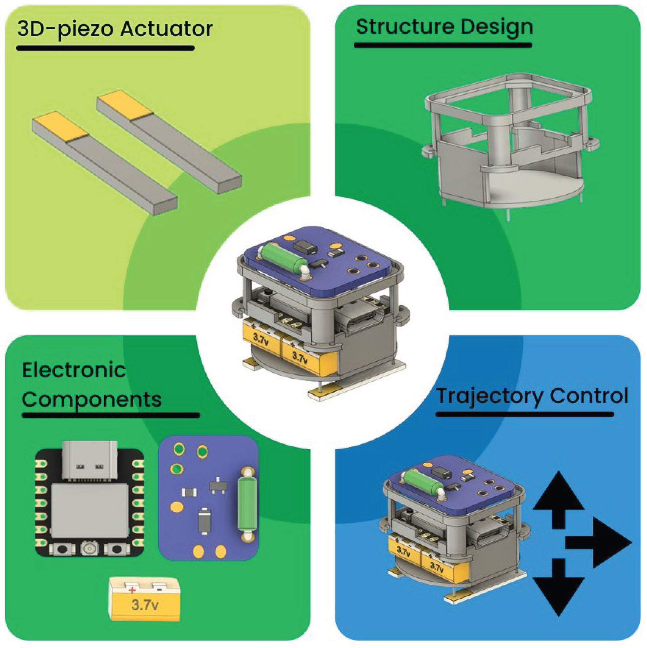
Figure 2.
(a) Plates A and B with PZT patches. (b) Legs (blue parts) on plates A and B for the generation of linear movements.
Figure 2.
(a) Plates A and B with PZT patches. (b) Legs (blue parts) on plates A and B for the generation of linear movements.
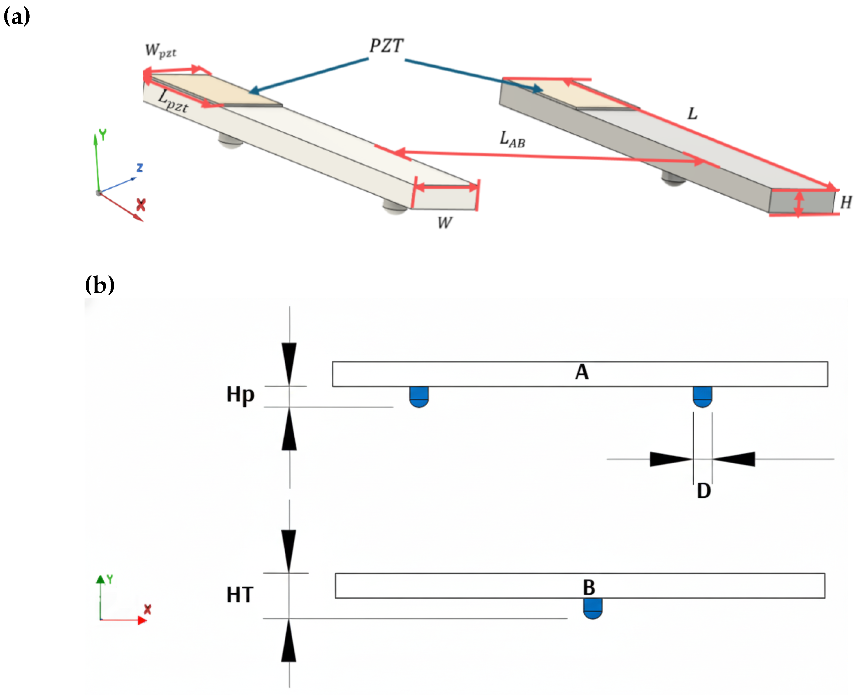
Figure 3.
FEM analysis of the piezoelectric plates showing the modal shape for the selected vibration modes. (a) Modal shape of (50) mode from the FEM simulation for Plates A and B, (b) Modal shape of (60) mode from the FEM simulation for Plates A and B.
Figure 3.
FEM analysis of the piezoelectric plates showing the modal shape for the selected vibration modes. (a) Modal shape of (50) mode from the FEM simulation for Plates A and B, (b) Modal shape of (60) mode from the FEM simulation for Plates A and B.
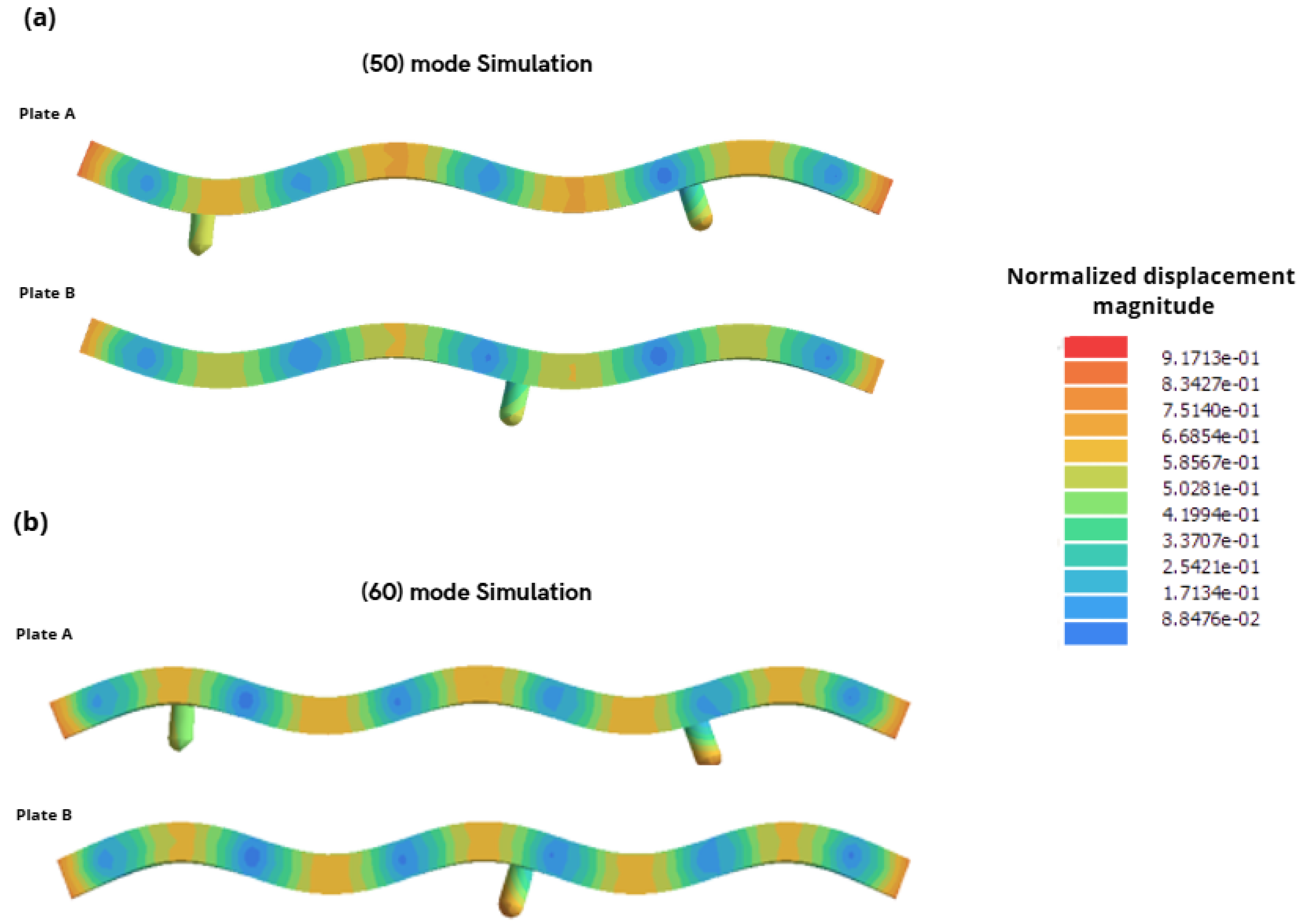
Figure 4.
Generation of the robot’s linear motion through standing waves (SW) using (50) and (60) modes [25].
Figure 4.
Generation of the robot’s linear motion through standing waves (SW) using (50) and (60) modes [25].
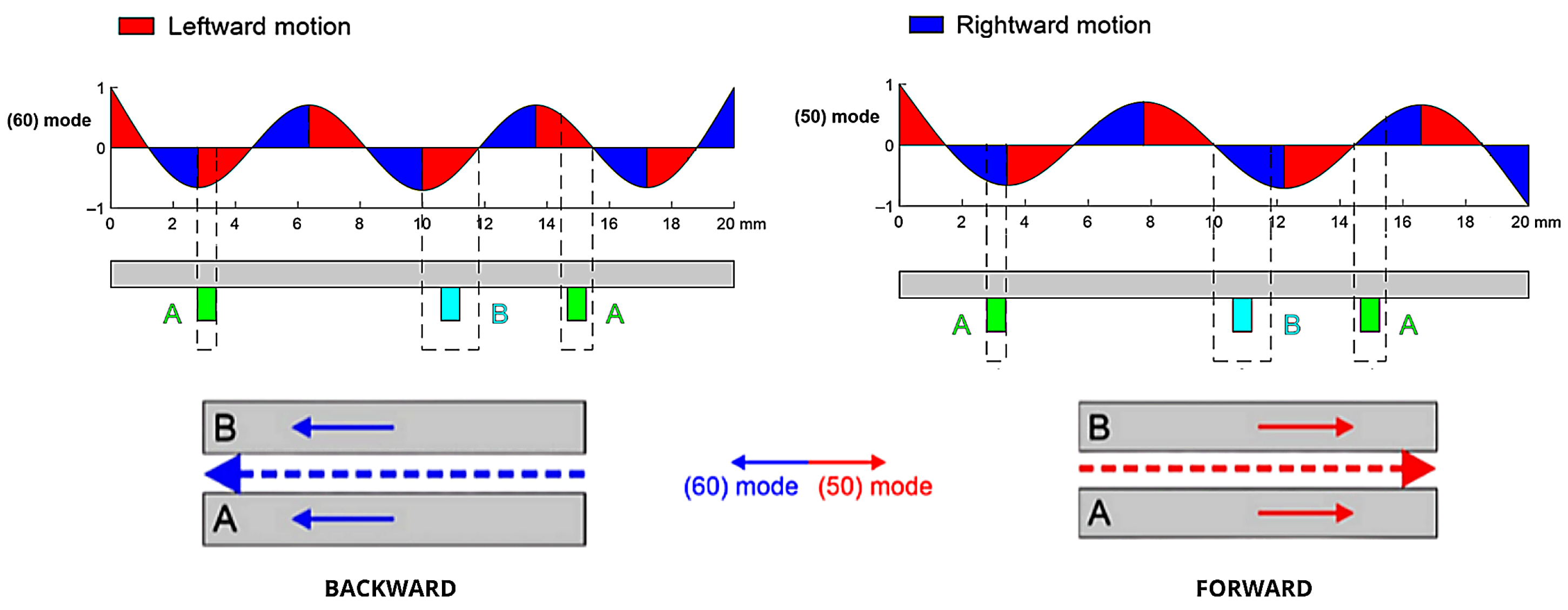
Figure 5.
Combination of (50) mode and (60) mode to generate rotational movements [25].
Figure 5.
Combination of (50) mode and (60) mode to generate rotational movements [25].
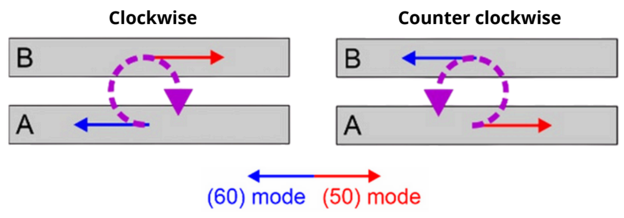
Figure 6.
Components of the miniature robot for trajectory control.
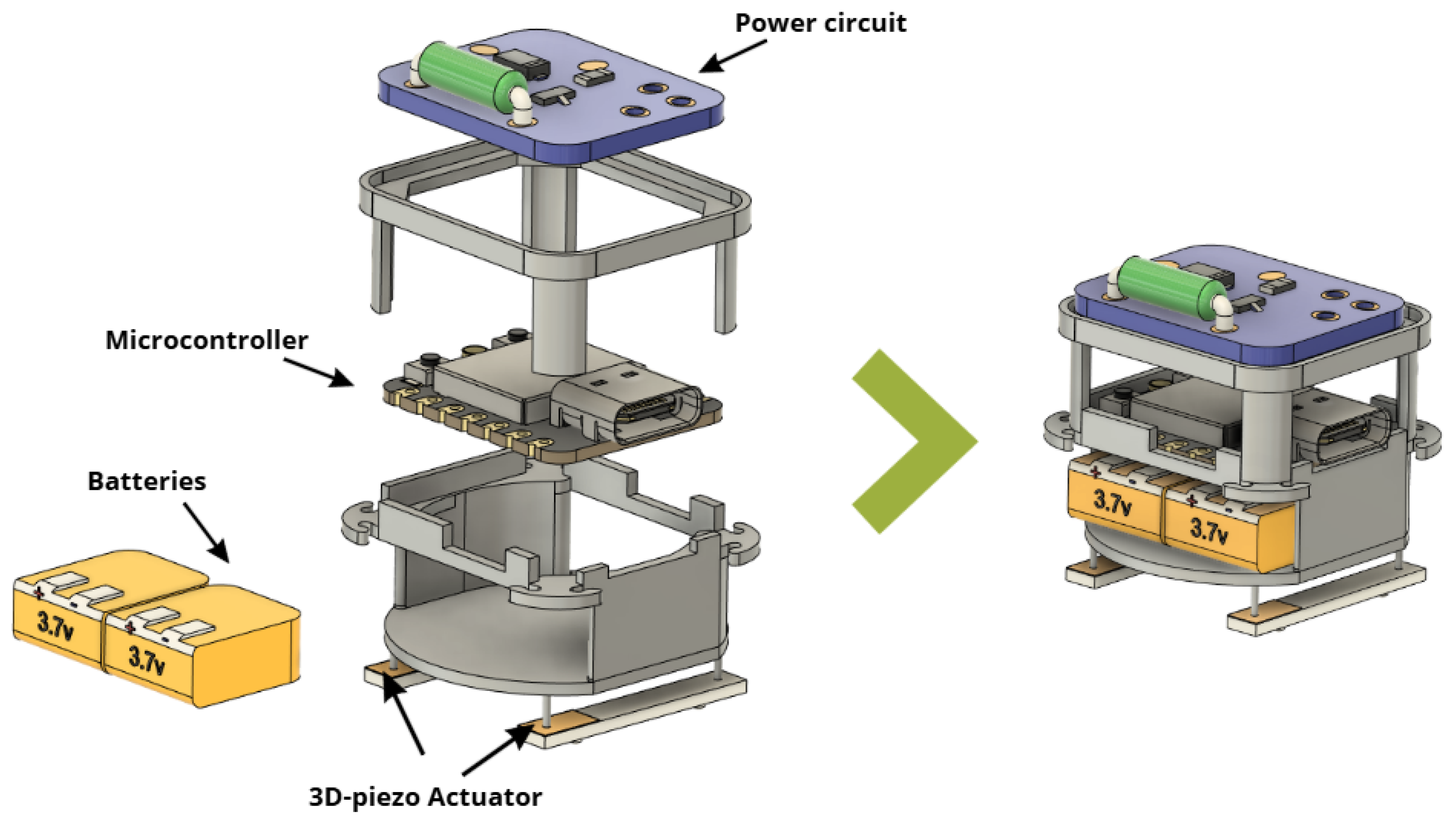
Figure 7.
Schematic diagram of the power circuit.
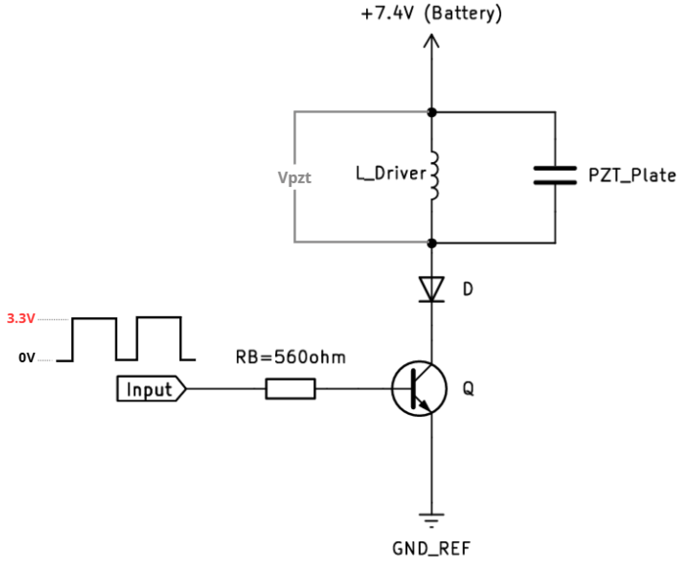
Figure 8.
Piezoelectric voltage and control signal (input) at 95 KHz and 50% duty cycle.
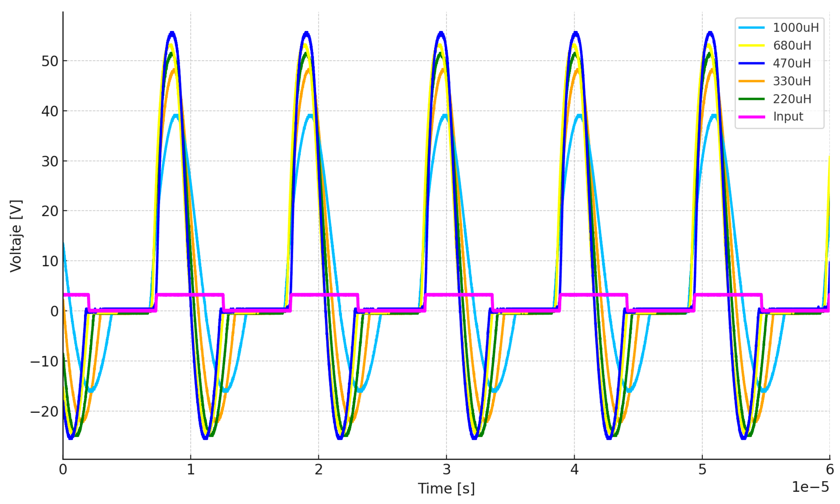
Figure 9.
Duty cycle variation between 40% and 75% to keep the current within the minimum and maximum limits that ensure proper operation of the piezoelectric actuators.
Figure 9.
Duty cycle variation between 40% and 75% to keep the current within the minimum and maximum limits that ensure proper operation of the piezoelectric actuators.
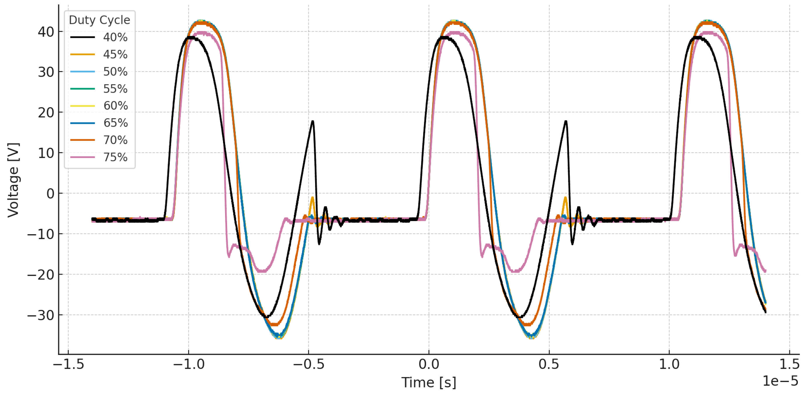
Figure 10.
Electronic schematics of the miniature robot.
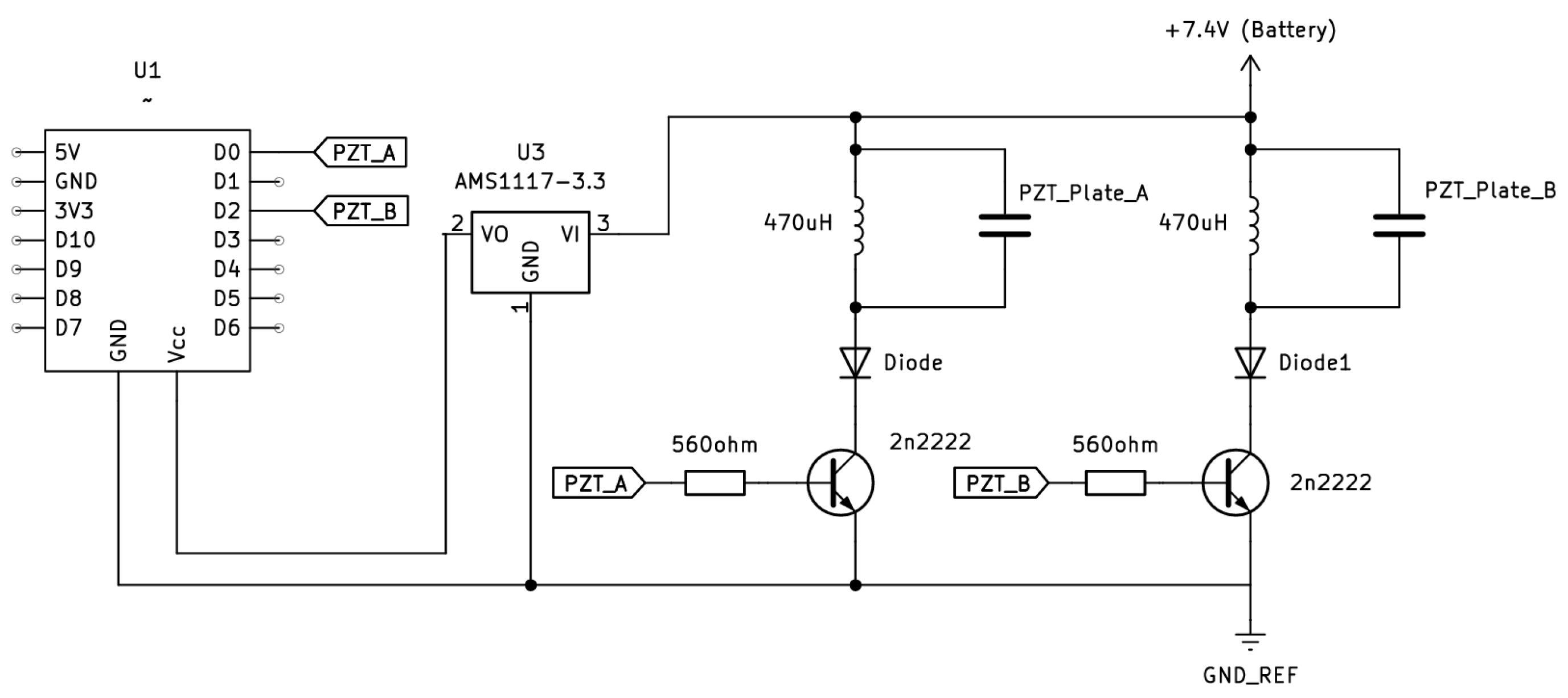
Figure 11.
Structural parts designed to accommodate the electronic components of the robot.
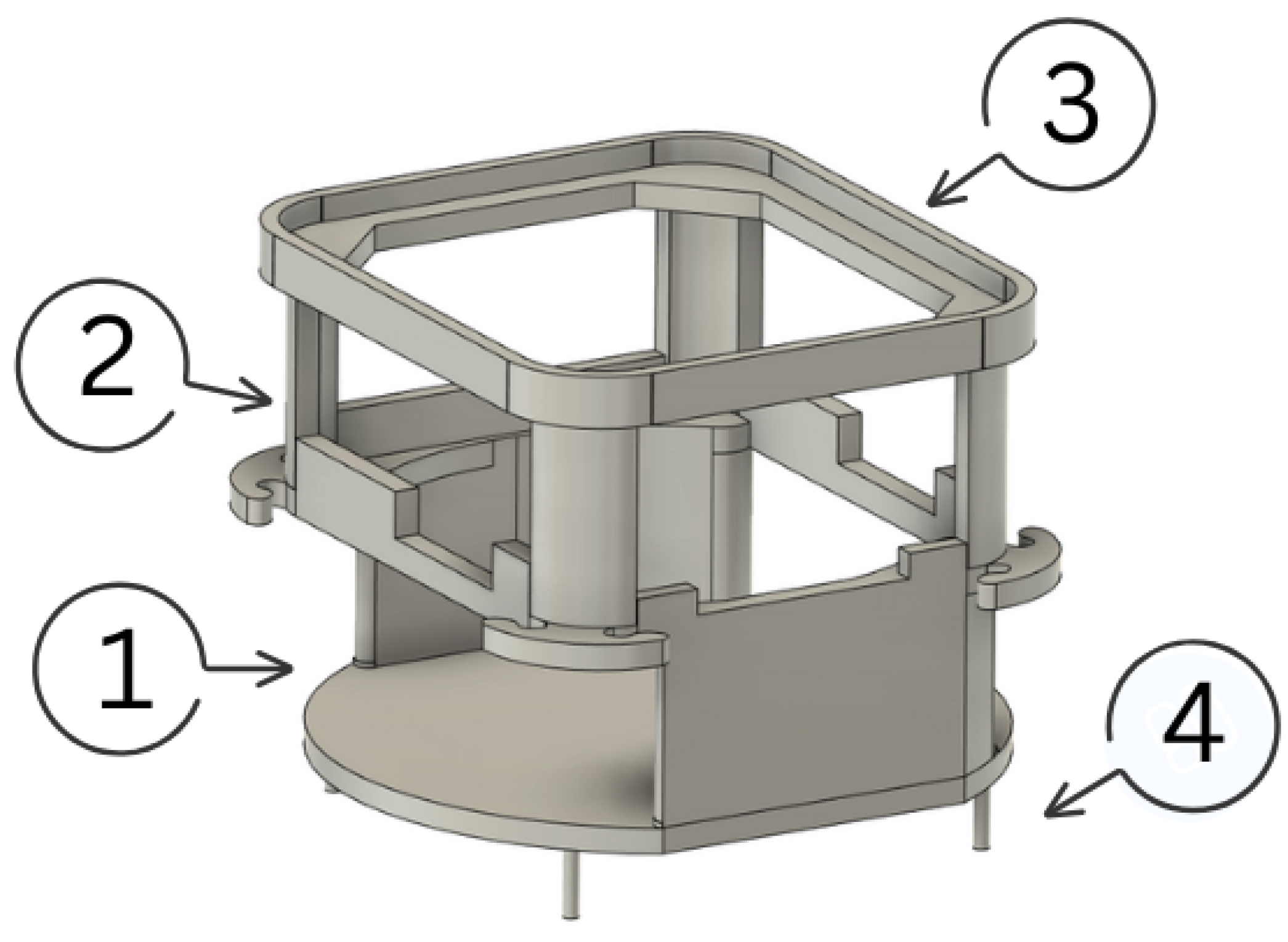
Figure 12.
Width, length, and height dimensions of the robot structure.
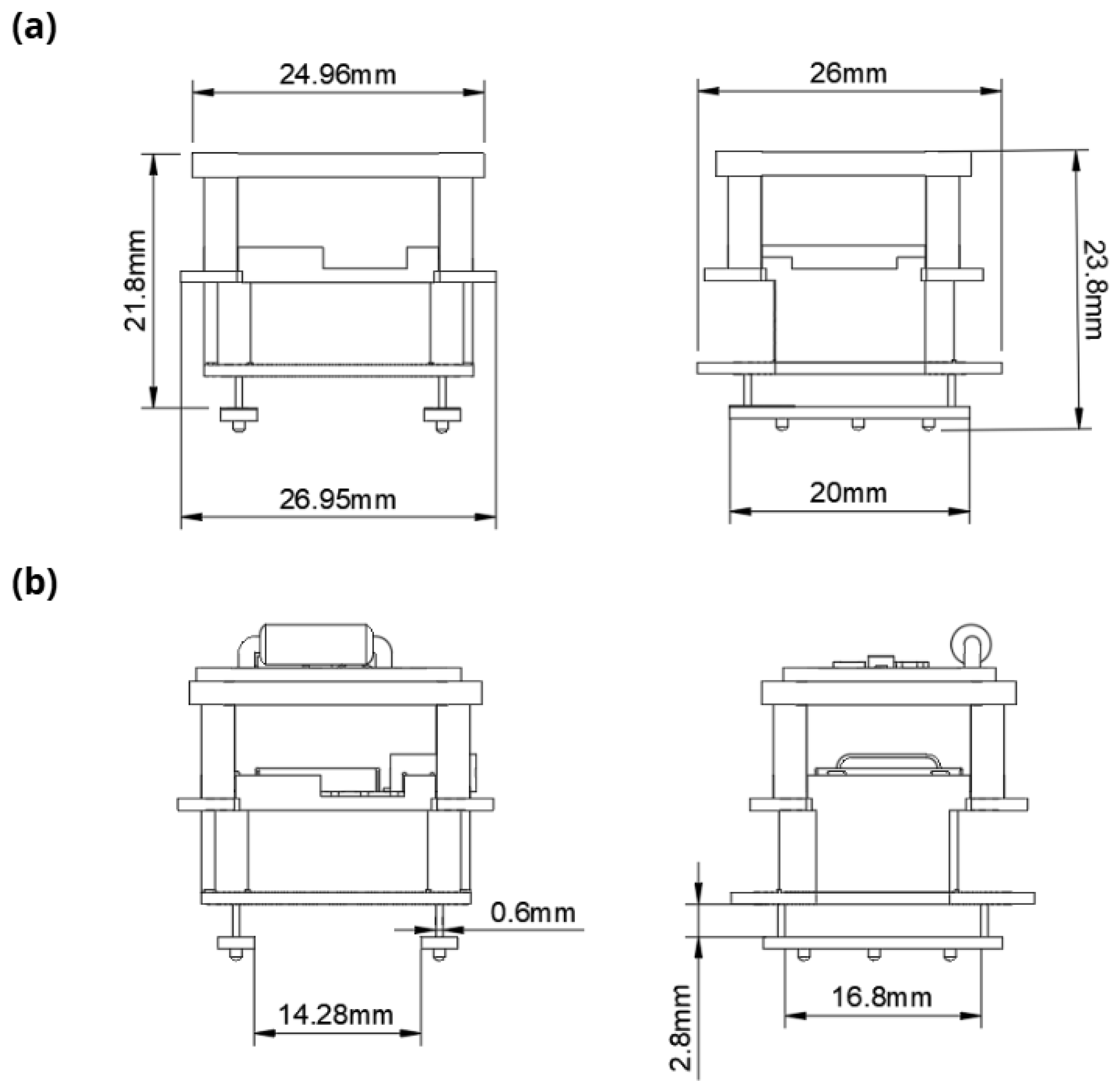
Figure 13.
Finite element analysis of the robot structure: (a) Static deformation under point loads equivalent to the microcontroller, piezoelectric driver PCB, and battery weights (scale in mm). (b) von Mises stress distribution in the supporting legs of the structure (scale in MPa).
Figure 13.
Finite element analysis of the robot structure: (a) Static deformation under point loads equivalent to the microcontroller, piezoelectric driver PCB, and battery weights (scale in mm). (b) von Mises stress distribution in the supporting legs of the structure (scale in MPa).
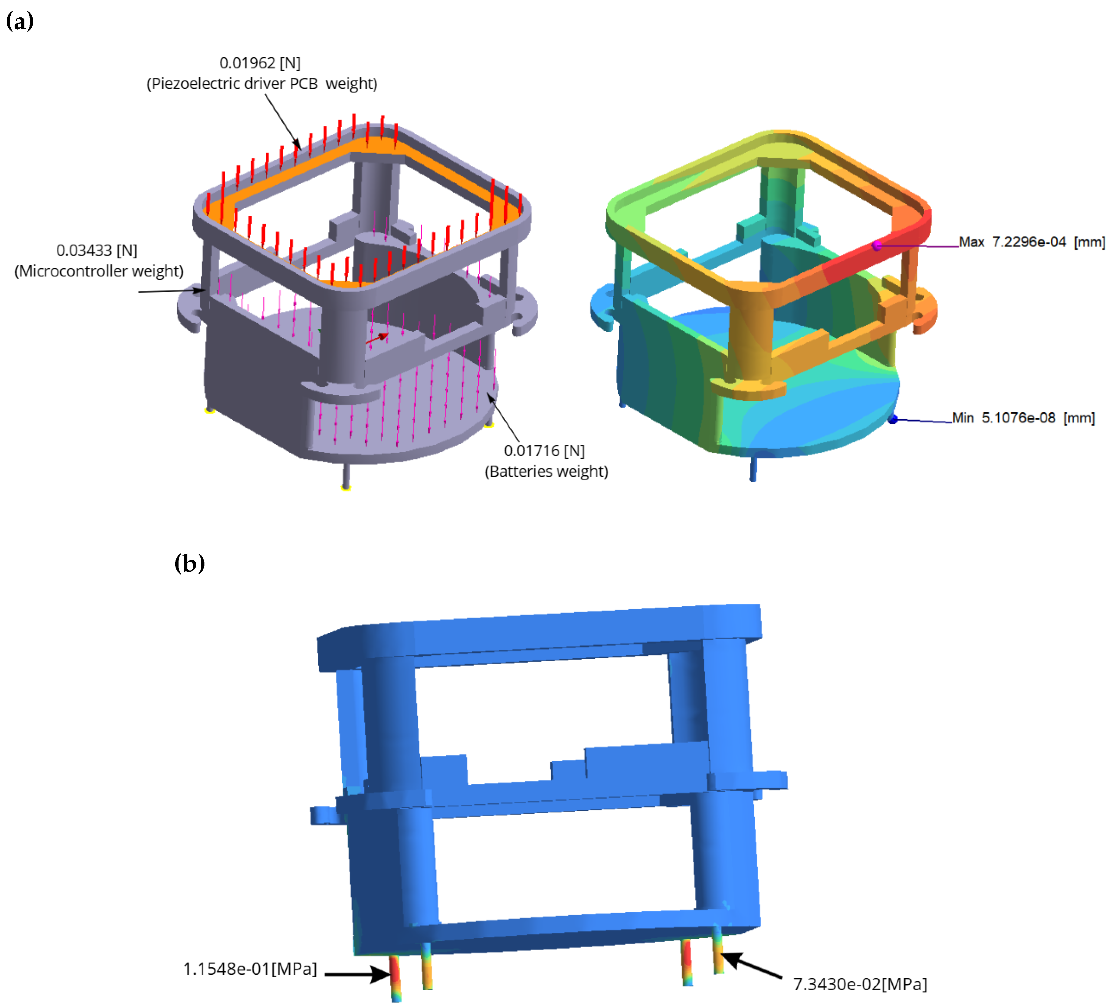
Figure 14.
Photographs of the assembled miniature robot: (a) Front view showing the structural frame and electronic components; (b) Oblique view of the miniature robot structure showing the arrangement of the electronic board and supporting plates A and B.
Figure 14.
Photographs of the assembled miniature robot: (a) Front view showing the structural frame and electronic components; (b) Oblique view of the miniature robot structure showing the arrangement of the electronic board and supporting plates A and B.
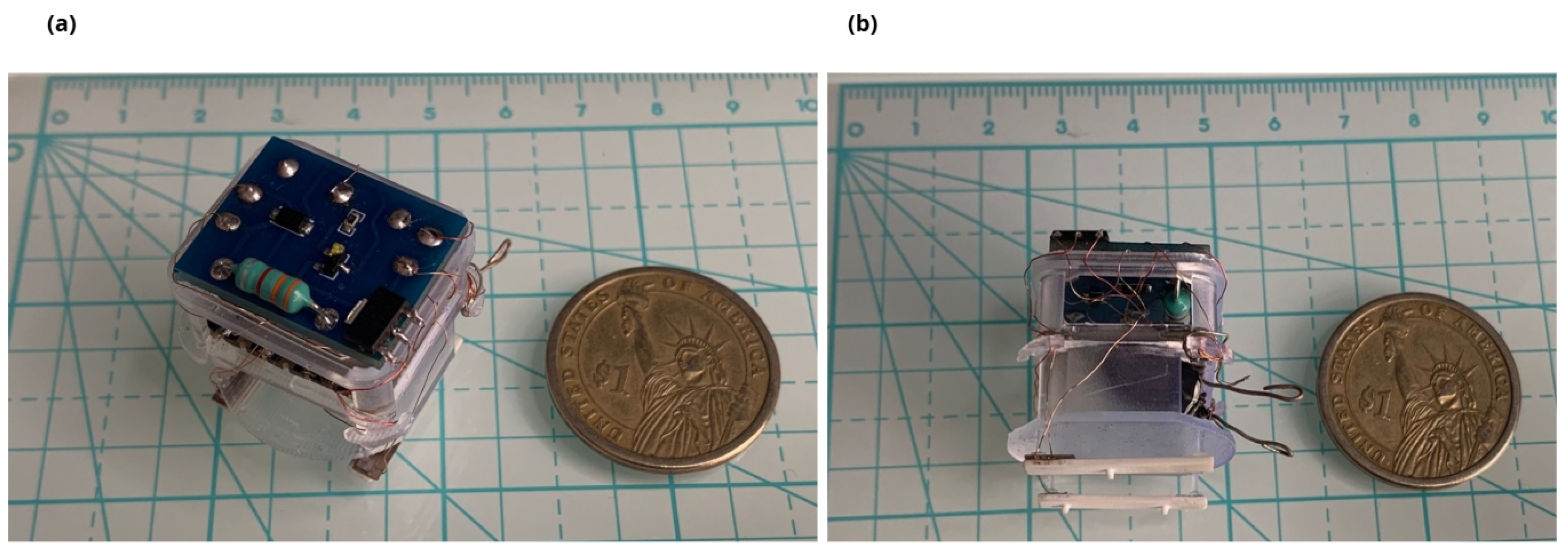
Figure 15.
Block diagram for the trajectory control of the miniature robot.
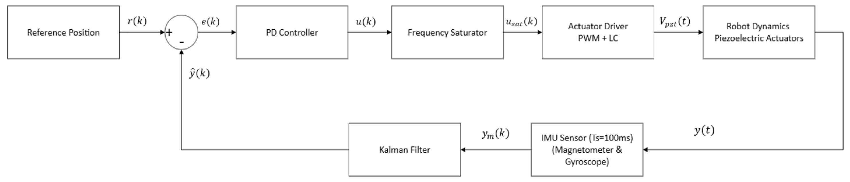
Figure 16.
Comparison between the gyroscope Z-axis signal without filtering (blue) and the signal filtered with the Kalman algorithm (orange) during the rest state, with no robot motion.
Figure 16.
Comparison between the gyroscope Z-axis signal without filtering (blue) and the signal filtered with the Kalman algorithm (orange) during the rest state, with no robot motion.
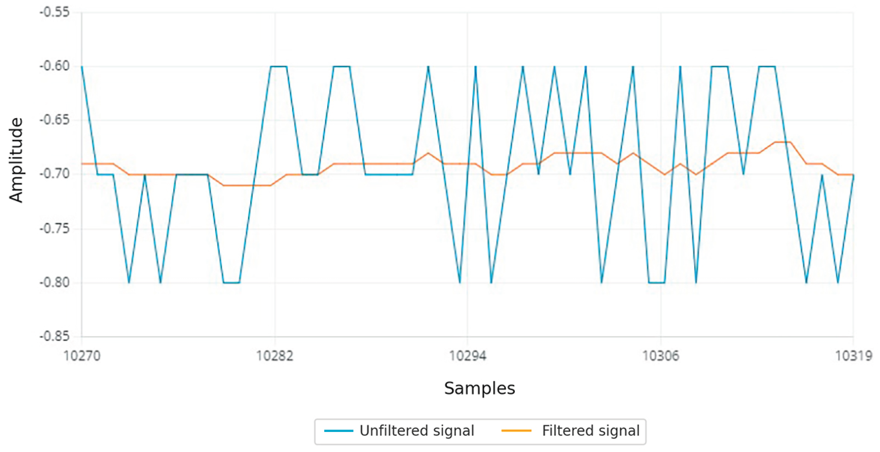
Figure 17.
Hysteresis curve for PD control showing the switching logic of actuators A and B during midpoint, positive phase (CCW), and negative phase (CW).
Figure 17.
Hysteresis curve for PD control showing the switching logic of actuators A and B during midpoint, positive phase (CCW), and negative phase (CW).
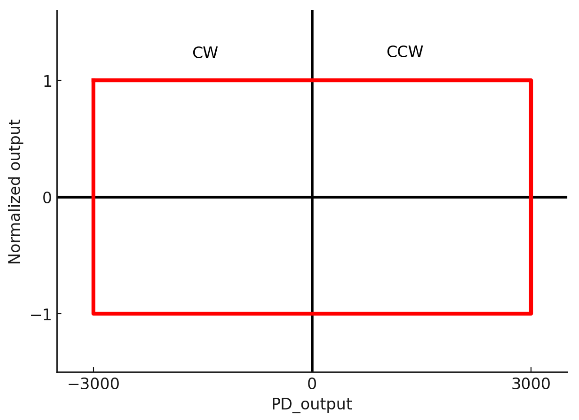
Figure 18.
Conductance vs. Frequency for Plate A and Plate B. Resonance peaks corresponding to (50) and (60) modes are identified.
Figure 18.
Conductance vs. Frequency for Plate A and Plate B. Resonance peaks corresponding to (50) and (60) modes are identified.
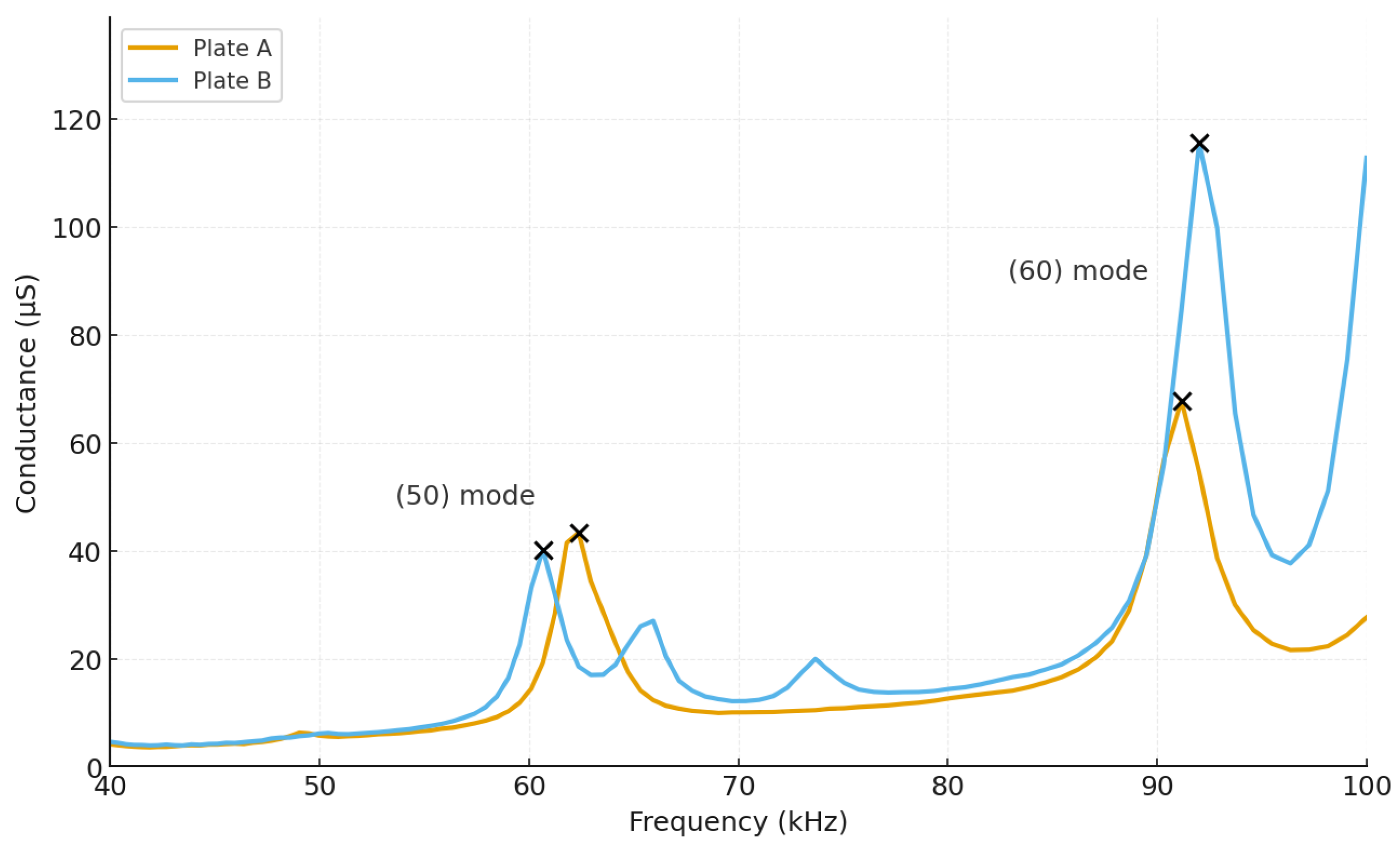
Figure 19.
Boxplots of the 20 mm linear displacement time and the 180° clockwise and counterclockwise rotation times ().
Figure 19.
Boxplots of the 20 mm linear displacement time and the 180° clockwise and counterclockwise rotation times ().
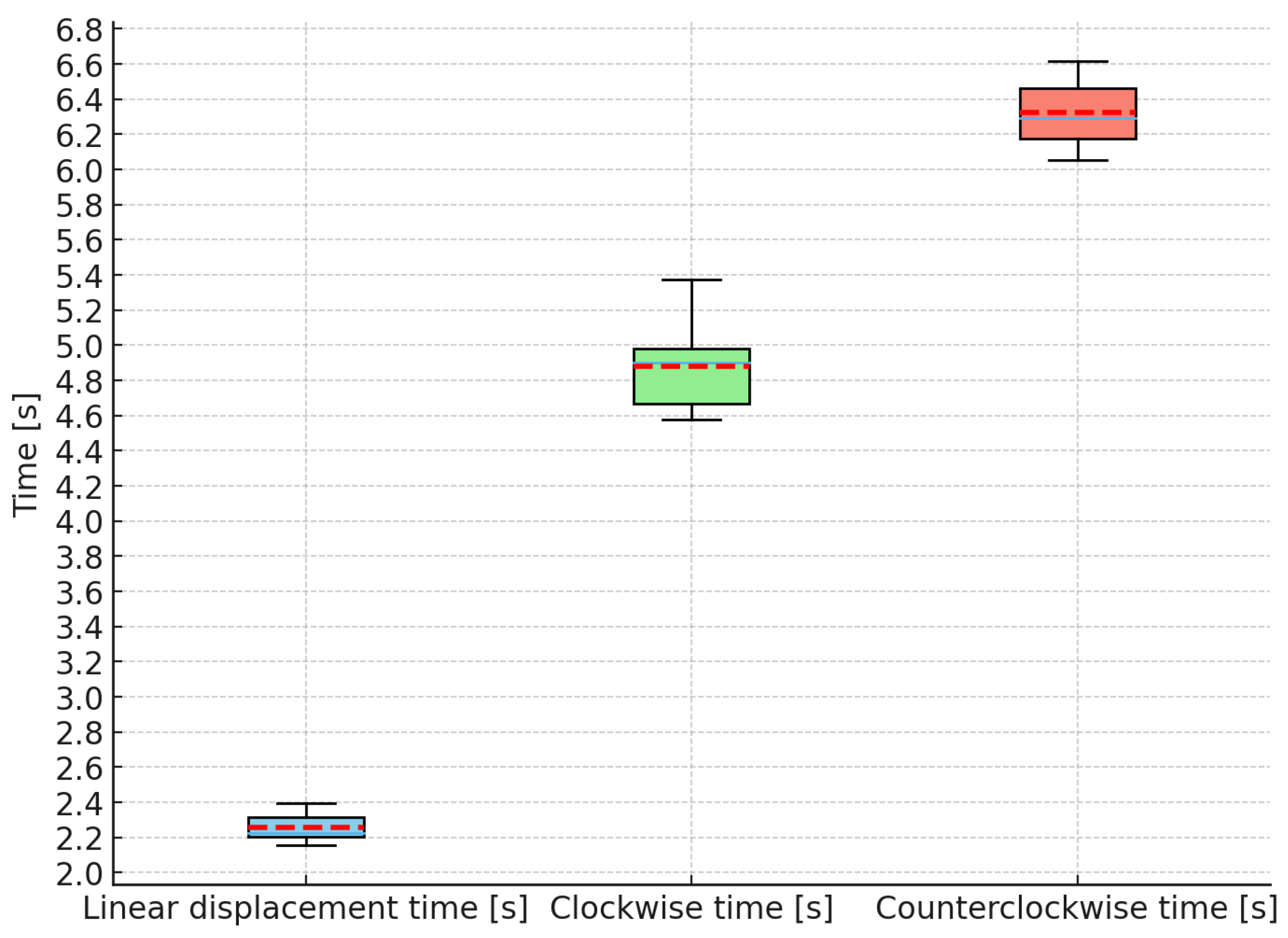
Figure 20.
Open-loop motion of the miniature robot under excitation at 60 kHz (65% duty cycle), and angular deviation of the robot measured with the gyroscope during open-loop operation. The experiment is shown in the supplementary video (Video S2).
Figure 20.
Open-loop motion of the miniature robot under excitation at 60 kHz (65% duty cycle), and angular deviation of the robot measured with the gyroscope during open-loop operation. The experiment is shown in the supplementary video (Video S2).
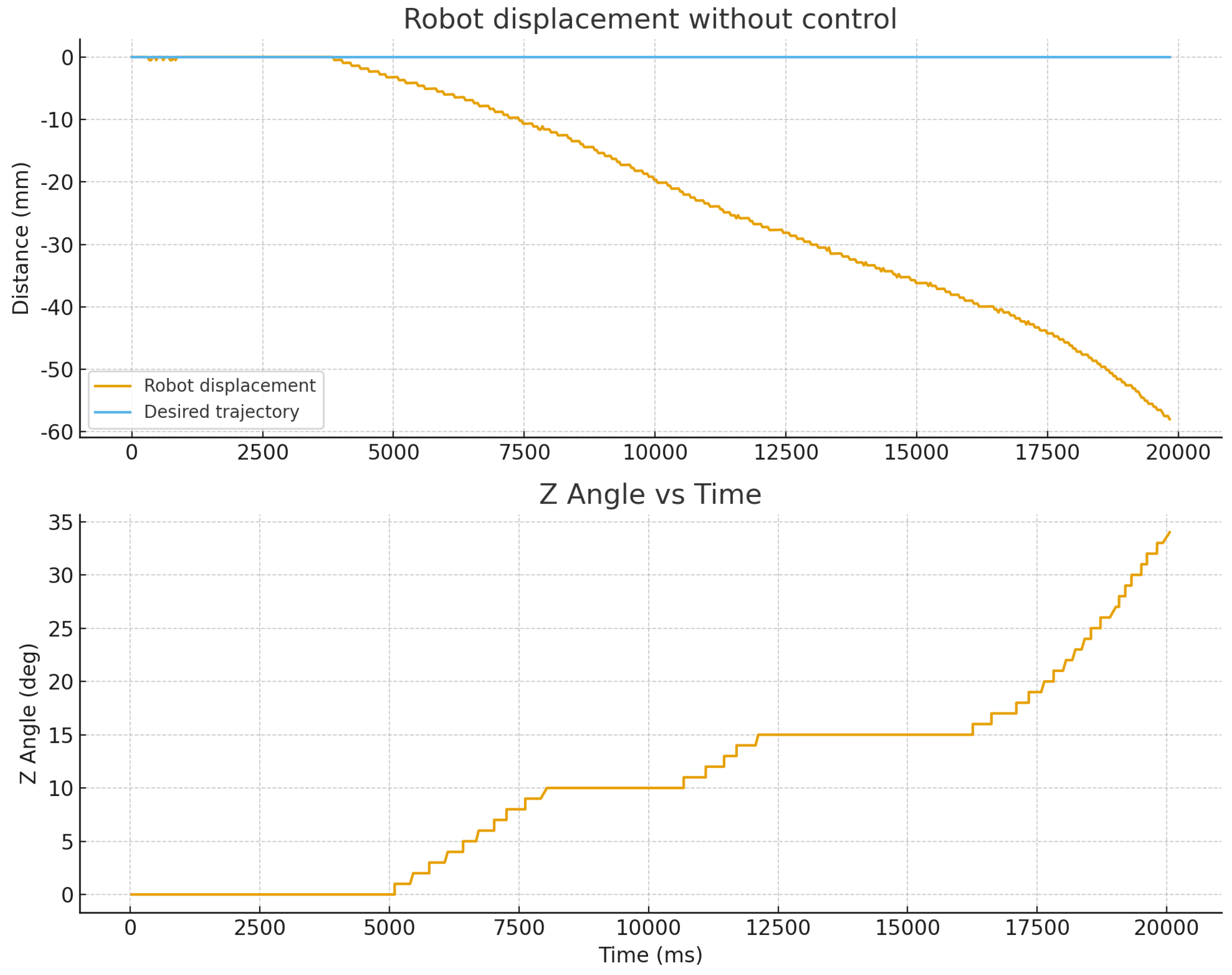
Figure 21.
Closed-loop trajectory control performance using a PD controller and closed-loop angular response obtained from the gyroscope output. The experiment can be observed in the supplementary video (Video S3).
Figure 21.
Closed-loop trajectory control performance using a PD controller and closed-loop angular response obtained from the gyroscope output. The experiment can be observed in the supplementary video (Video S3).
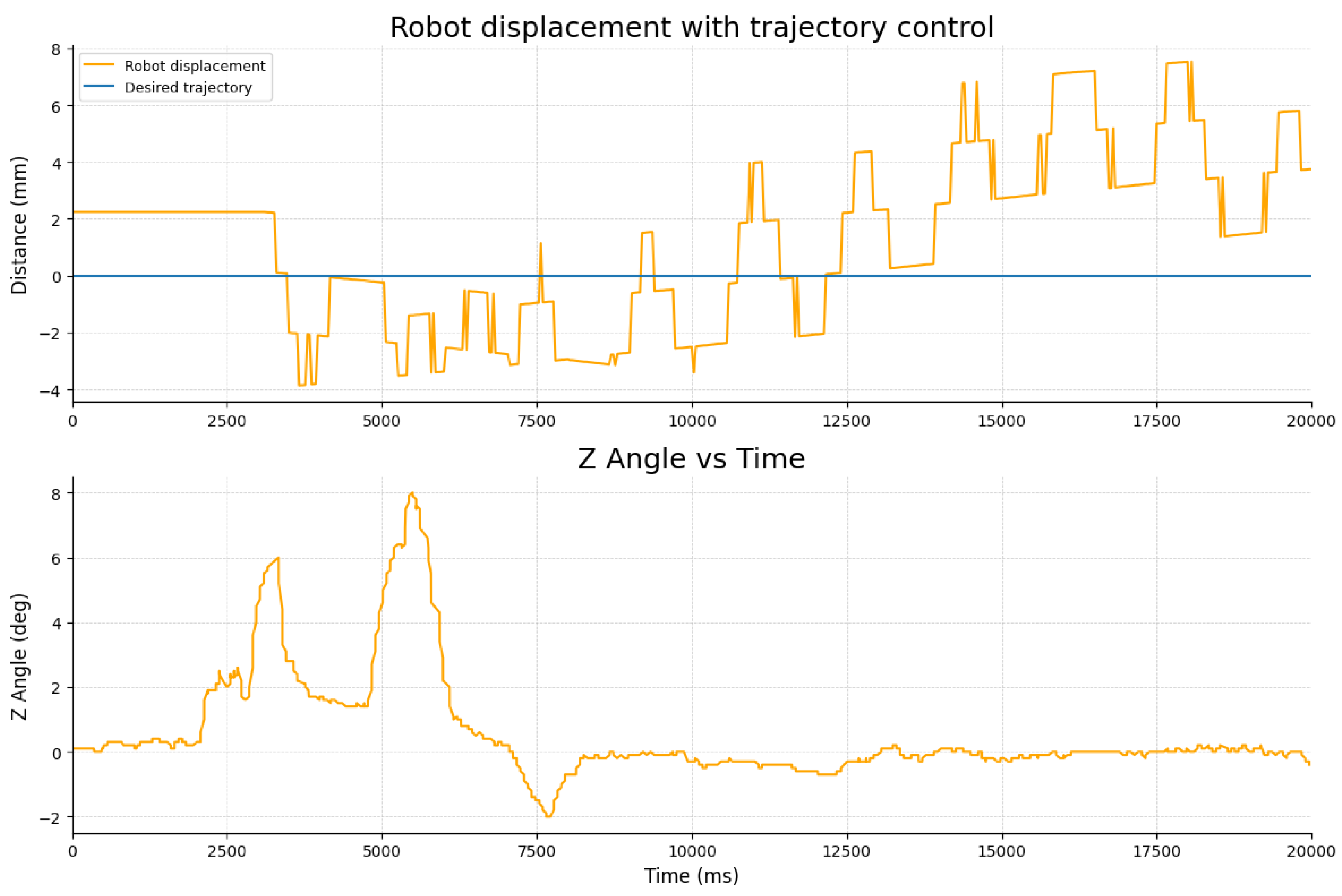
Figure 22.
Control signal applied to actuators A and B as a function of time.
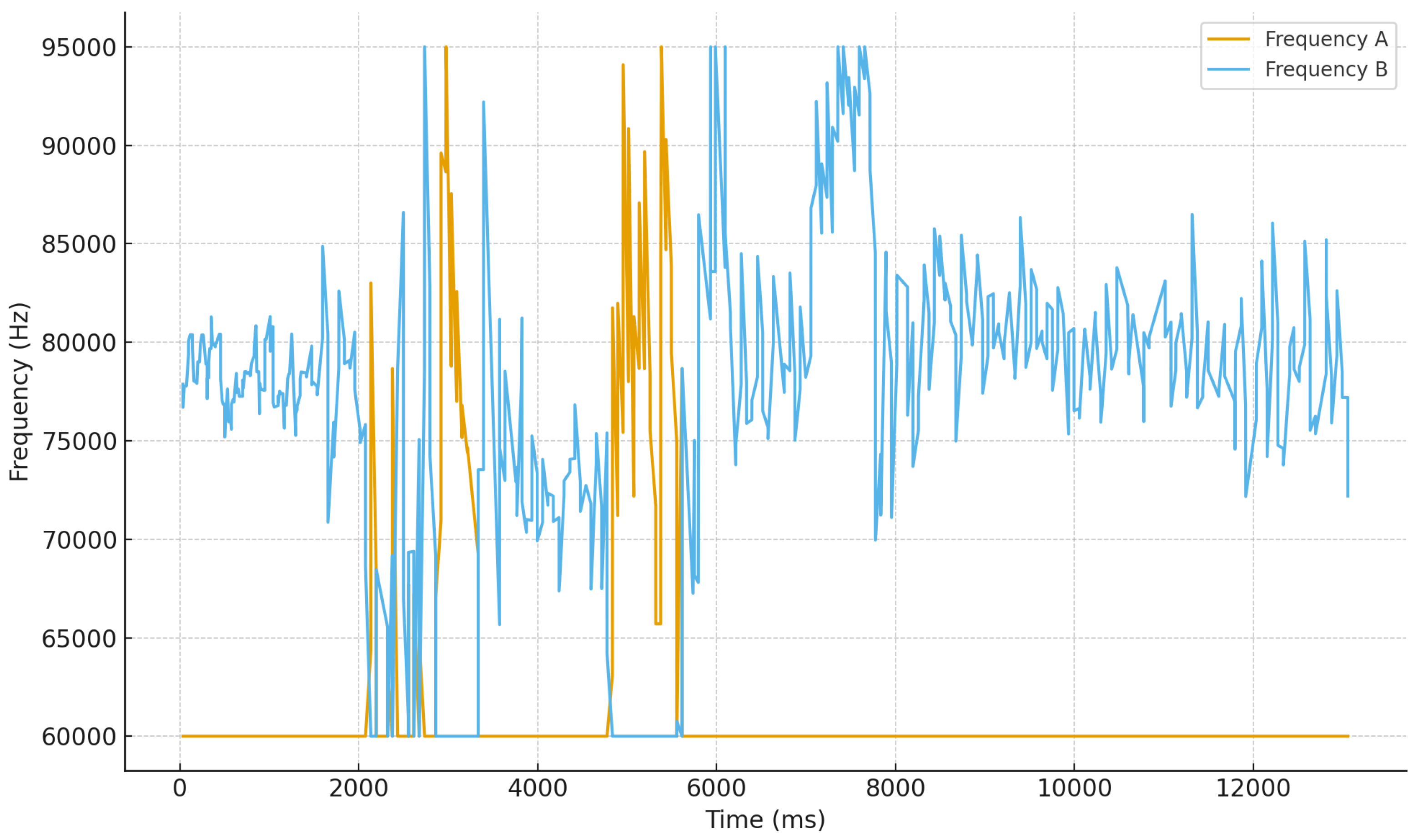

Table 1.
Main Properties of the Piezoelectric Material PIC 255 [22].
Table 1.
Main Properties of the Piezoelectric Material PIC 255 [22].
| Parameter | Unit | PIC 255 |
|---|---|---|
| Density | g/cm3 | 7.8 |
| Mechanical Quality Factor () | – | 80 |
| Piezoelectric Deformation () | pm/V | -180 |
| Piezoelectric Deformation () | pm/V | 390 |
| Piezoelectric Deformation () | pm/V | 500 |
| Piezoelectric Voltage Coefficient () | 10-3 Vm/N | -11.5 |
| Piezoelectric Voltage Coefficient () | 10-3 Vm/N | 28 |
| Elastic Compliance Coefficient () | 10-12 m2/N | 15.3 |
| Elastic Compliance Coefficient () | 10-12 m2/N | 5.5 |
| Elastic Stiffness Coefficient () | 1010 N/m2 | 20.7 |
| Elastic Stiffness Coefficient () | 1010 N/m2 | 7.4 |
Table 2.
Tested inductors and corresponding electrical response.
| Inductor (uH) | (KHz) | (V) | (A) |
|---|---|---|---|
| 1000 | 118.63 | 55.2 | 0.01 |
| 680 | 143.86 | 78 | 0.02 |
| 470 | 173.04 | 81.2 | 0.03 |
| 330 | 206.50 | 70.4 | 0.07 |
| 220 | 252.91 | 76.4 | 0.1 |
Table 3.
Specifications of the Li-Po 401010 Battery [31].
Table 3.
Specifications of the Li-Po 401010 Battery [31].
| Feature | Li-Po 401010 Battery |
|---|---|
| Dimensions | 4 × 10 × 10 mm |
| Weight | ~0.6 g |
| Typical Capacity | 30 mAh |
| Nominal Voltage | 3.7 V |
| Operating Temperature | –20°C to +60°C |
| Life Cycle | 300 – 500 charge cycles |
Table 4.
Dimensions and weight of the electronic components that constitute the miniature robot.
| Element | Quantity | Mass | Dimension |
|---|---|---|---|
| Microcontroller | 1 | 3.5 g | 21 × 17.5 × 5 mm |
| Piezoelectric driver PCB | 1 | 2 g | 22.2 × 18 × 10 mm |
| Batteries | 2 | 1.5 g | 4 × 10 × 10 mm |
| 3D-piezo Actuators | 2 | 0.2 g | 3 × 20 × 0.8 mm |
| Total | 6 | 7.2 g | – |
Table 5.
Values used for the initialization of the Kalman filter.
| Variable | Value |
|---|---|
| 0 | |
| 1 | |
| Q | 0.01 |
| R | 100 |
Table 6.
Conductance measurement results for plates A and B in (50) and (60) modes.
| Plate | (50) mode | (60) mode | ||
|---|---|---|---|---|
| Frequency [kHz] | Conductance peak [S] | Frequency [kHz] | Conductance peak [S] | |
| A | 62.37 | 43.4 | 91.16 | 67.8 |
| B | 60.67 | 40.2 | 92.01 | 115.7 |
Table 7.
Trajectory deviation metrics in open-loop condition.
| MAE | RMSE | Max |
|---|---|---|
| 9.79° | 13.01° | 34° |
Table 8.
Trajectory deviation metrics in closed-loop condition.
| MAE | RMSE | Max |
|---|---|---|
| 0.83° | 1.73° | 8° |
Disclaimer/Publisher’s Note: The statements, opinions and data contained in all publications are solely those of the individual author(s) and contributor(s) and not of MDPI and/or the editor(s). MDPI and/or the editor(s) disclaim responsibility for any injury to people or property resulting from any ideas, methods, instructions or products referred to in the content. |
© 2025 by the authors. Licensee MDPI, Basel, Switzerland. This article is an open access article distributed under the terms and conditions of the Creative Commons Attribution (CC BY) license (http://creativecommons.org/licenses/by/4.0/).
Copyright: This open access article is published under a Creative Commons CC BY 4.0 license, which permit the free download, distribution, and reuse, provided that the author and preprint are cited in any reuse.


