
Submitted:
28 November 2025
Posted:
28 November 2025
You are already at the latest version
Abstract
This paper investigates the influence of environmental, social, and governance (ESG) factors on financial development, using Domestic Credit to the Private Sector by Banks (DCB) as the core indicator of credit market development. To effectively market the research within the broader literature on finance and ESG issues, the authors employ an approach combining econometric analysis, K-Nearest Neighbors (KNN), cluster analysis, and network analysis. By analyzing the impact through the estimation of the model parameters through the impact of instrumental variable estimation on the model parameters (using Two-Stage Least Squares (IV), Random Effects (IV), and First-Differenced (IV) methods), the study confirms that access to clean fuels and natural resource depletion impact the model margins significantly. However, across all the models used in the analysis, the impact of access to clean energy is positive. By analyzing the significance of the issue using the KNN model throughout the research process on the impact of ESG on credit market dynamics across countries, the research demonstrates that the issue is significant. By performing hierarchical cluster analysis on the significance of the research by considering the significance of the issue in its contribution to the impact on credit market dynamics in countries, in terms of climate stress issues being core in influencing the dynamics of credit in countries, through network analysis mapping performed by carrying out research on the topic.
Keywords:
ESG
; financial development
; domestic credit
; sustainability
; environmental indicators
1. Introduction
One of the most prevalent strands in the literature on contemporary economic studies concerns the interplay between the environmental, social, and governance (ESG) framework and the evolution of financial systems across countries. The impact of climate transition, institutional upgrading, and social integration paradigms (Bruno & Henisz, 2024) in the face of the mounting pressures for climate transition suggests that the dynamics for credit allocations in the evolving financial regimes in the aftermath of the climate imperatives indicate that the resource allocations in credit terms are no longer governed by the enduring pure economic tenets. However, as opposed to the countervailing forces of ESG (Chodnicka-Jaworska, 2022). Domestic Credit to the Private Sector by Banks (DCB), the index typically used in context to the advancement of the financial system in terms of its forward ability for the generation of economic infrastructure through the enabling power of the credit institutions on the constituents’ behalf, presents an interesting paradigm in the analysis on what the determinants in the context of the contribution by the ESG framework (governance paradigm on the one aspect related to environmental quotient (Evans, Kramer, Lanfranchi, & Brijlal, 2023). This work will make its contribution to the literature by briefly analysing the degree to which ESG issues affect financial development dynamics in various countries through the use of an inter-method analysis approach combining the strengths of econometric model analysis, Machine Learning methods, cluster analysis, and network analysis (Mohapatra, Das, Nayak, Sahoo, & Matta, 2025). Meanwhile, the rising paradigm of sustainable finance in the international context profoundly impacted the dynamics of finance in the environment (You, Chen, Fang, Gao, & Cheng, 2024). Thus, in the new paradigm of finance amid the global shift toward environmentally positive transition, financial institutions must now adapt to climate risks in their operations by factoring environmentally sound factors into loan disbursements (Chen, Lakkanawanit, Suttipun, Swatdikun, & Huang, 2024). Clean energy accessibility, biodiversity depletion, emissions profiles, climate stress measures, natural resource pressures, and the like are among the factors that might influence the future outlook for incentives, constraints, and expectations in the financial market. Social/governance aspects of ESG considerations like the regulation framework of the nation, the level of education in the region, the institutionalization of rights in the social context, and the infrastructure of knowledge might influence the ability of the region towards the maintenance of financial developments within the framework of environmentally sustainable transition processes (Cioli, Giannozzi, Pescatori, & Roggi, 2023). Governance capabilities might influence the stability of financial institutions. Notwithstanding the recent recognition of the linkages between environmental systems and financial regimes, the literature on the topic is scattered in its empirical observations. This is because the current body of research employs the one-dimensional approach to address finance-sustainability linkages, using a conventional econometric framework that lacks the ability to capture the complexity of these relationships (Ding et al. 2024). Additionally, the literature employs a multi-feature framework of the environment because access to green energy sources may increase financial inclusion in some nations. However, the depletion of natural resources within the same nations might reduce credit access within those countries due to climate-related shocks. To explore the linkages in the literature, the research will harness joint ESG determinants of DCB by utilising the approach that combines methodological structures adept at identifying causalities in the context of mapping the structural aspects (Dai et al. 2025). To begin the analysis, the research uses instrumental variable models to address endogeneity in the interaction between financial development and environmental factors. Indicators of the environment, such as access to clean fuels, natural resource depletion, and carbon emissions, could affect one another simultaneously in response to the performance of the economy and the institutions in place. By considering distributional heterogeneity through the First-D Differenced IV estimations, Two-Stage Least Squares analysis, and Random Effects Models for IV analysis, the research accounts for structural heterogeneity. Access to clean fuels is consistently evaluated as a positive determinant of DCB across all model structures. Natural resource depletion adversely affects financial DCB, underscoring the importance of ecological sustainability in the context of the research (You et al., 2024). Emissions in the research act differently according to the models used. In addition to the econometric model, the research uses machine learning capabilities to gain better insight into the importance of the structure in DCB estimation. Among the models used in the analysis, the K-Nearest Neighbours model yields the best results in terms of estimation. KNN achieves near-exact estimation during the validation process (Mohapatra et al., 2025). Compared to other estimation methods, such as regression, K-Neighbours allows better adaptation to local structures in high-dimensional data. K-Neighbours estimation captures the influence of different environmental structures on the credit system in the observation period. The analysis of the importance of the dropout loss function indicates that the primary determinants influencing the estimation of DCB are land-use indicators, climate-related stressors, the pressure of biodiversity loss on the environment, and the economy's emissions intensity (Zioło et al., 2023). Machine learning analysis supports the claim that financial systems are integrated into multivariate environmental regimes. Among the different structures of the observation period, land productivity measures, the significance of ecological conservation measures within the credit system framework, levels of environmental pollutants in the observation period, and the climate within the credit system approach affect the credit allocation mechanism (Bruno & Henisz, 2024). However, the use of clustering algorithms further deepens the analysis by identifying distinct regimes corresponding to different types of financial development. Hierarchical clustering, in particular, stands out as the most accurate approach for grouping countries based on environmental factors. This is according to the Silhouette values, index of separation, and the index of the Dunn method (Ding et al., 2024). The clusters also exhibit some diversity in terms of natural environmental features, in that some countries are in a single large pool that does not closely represent the average environment, while others are in small, distinct clusters that exhibit varying degrees of natural stress. Finally, network analysis reveals the system-level dynamics of the interconnectivity among environmental variables and their structural association with DCB. That the network exhibits low sparsity and high interconnectivity indicates that environmental factors act not independently but rather as part of an integrated system (Dai et al., 2025). Climate-related stress variables, such as high temperatures, emissions indicators, and biodiversity-related measures, play key roles in the network by mediating the interconnectivity between land use patterns, energy access measures, and ecological stress (Chen et al., 2024). By combining diverse empirical methods, the research presents a comprehensive framework for analysing the impact of ESG factors on the evolution of the domestic credit market. Based on the research results, the process of financial development cannot be fully explained without considering the environmental context in which national economies operate (Evans et al., 2023). According to the research results, the course of sustainable financial development should involve implementing comprehensive programs to improve environmental quality, enhance institutional quality, and strengthen social capacity (Cioli et al., 2023). Such comprehensive research on the implementation of the multimethod approach demonstrates that financial development across countries is influenced by diverse environmental factors through various causal relationships (Chodnicka-Jaworska, 2022). Hence, the process of implementing financial policy within the ESG framework requires consideration of the multidimensionality of the impact of the studied variable. This research work makes a contribution to the paradigm shift in the field of financial development in the context of an increasingly specialised world shaped by the logic of sustainable development (You et al., 2024).
2. Literature Review
The selected articles collectively highlight the growing relevance of ESG dimensions in shaping financial systems, yet they differ markedly from the approach adopted in the attached study, both methodologically and conceptually. Many of the papers—such as Abdelfattah et al. (2025) and Adebiyi et al. (2025)—rely heavily on machine learning to identify ESG performance determinants, but they typically focus on firm-level or national sustainability performance rather than on how ESG factors influence financial development itself. In contrast, the attached article adopts a multimethod strategy combining econometrics, KNN-based machine learning, hierarchical clustering, and network analysis to isolate environmental and institutional factors driving Domestic Credit to the Private Sector (DCB), providing a far more granular and systemic analysis. Acharya (2023) and Boström & Hannes (2024) emphasize the broad role of sustainable finance and climate-aligned investment flows but do not empirically model credit allocation. Their analyses remain conceptual, whereas the attached work demonstrates empirically that variables such as clean energy access, resource depletion, and governance significantly shape credit depth. Similarly, Alharbi (2024) and Chernykh et al. (2024) link ESG reforms and financing instruments to macroeconomic performance, yet they do not offer the integrated ESG–credit architecture developed in the attached study. Articles focusing on political stability, financial inclusion, or governance—such as Aich et al. (2025) and Alhassan et al. (2024)—provide important institutional insights but typically examine single channels in isolation. Conversely, the attached article demonstrates through network analysis that credit development is embedded in a dense system of environmental and governance interdependencies, a contribution absent from the compared literature. The review by Capoani (2025) maps ESG applications to territories but lacks causal estimation, while Alvarez-Perez & Fuentes (2024) explore ESG disclosure in debt markets without addressing the structural environmental drivers captured in the attached study. Likewise, Arnone et al. (2024) discuss access to credit within ESG frameworks but do not employ the multimethod triangulation that characterizes the attached work. Del Sarto and Ozili (2025) adopt a bibliometric methodology to map the intellectual structure of FinTech and financial inclusion research, highlighting digitalisation and innovation as drivers of access. Their macro-orientation contrasts with the attached study’s granular modeling of how environmental, social, and governance indicators shape domestic credit to the private sector through econometrics, machine learning, clustering, and network analysis. El Khoury et al. (2023) and Lamanda & Tamásné (2025) examine ESG determinants and disclosure in the banking sector, emphasizing institutional transparency and governance practices. While both stress governance quality as foundational for financial depth, they primarily assess ESG from the viewpoint of banks’ internal practices. The attached study instead models governance as an exogenous structural driver influencing credit allocation across countries, using instrumental variables to isolate causality. Farhoud (2025) foregrounds institutional voids and corporate sustainability in MENA contexts, revealing generational and cultural dynamics often absent from quantitative cross-country ESG analyses. Similarly, Guo & Naseer (2025) highlight financial inclusion, innovation, and development as pathways to ESG readiness, whereas the attached study positions ESG metrics not as outcomes but as determinants of financial development. Hassani et al. (2024) also explore the link between financial development and ESG globally, but focus more on correlation than causal pathways, which the attached work addresses through IV estimation. Studies such as Kandpal et al. (2024), Lotsu (2024), and Malik & Sharma (2025) emphasize sustainable finance instruments and corporate-level ESG impacts. These approaches differ markedly from the attached paper’s system-level modelling of DCB. Meanwhile, Lee et al. (2024) focus on microcredit and poverty alleviation, an angle distant from cross-country credit depth analyses but relevant for understanding the social component of ESG. Finally, McHugh (2023) investigates bankability of SDG projects, engaging with private-sector perceptions, whereas the attached manuscript uses quantitative environmental and governance indicators to trace structural determinants of credit distribution. Together, these contrasts demonstrate how the attached study diverges methodologically and conceptually through its systemic, multimethod, and causally oriented design. Mhlanga and Adegbayibi (2024) focus on Sub-Saharan Africa and emphasise regulatory frameworks, institutional capacity and market infrastructure as preconditions for sustainable finance. Their perspective is largely policy- and practice-oriented and treats financial development as an enabler of ESG, whereas the attached paper inverts the direction and empirically tests whether ESG conditions act as structural determinants of financial development, specifically domestic bank credit. A similar inversion appears in Miletkov and Staneva (2025), who analyse how equity and credit market development affect corporate social responsibility. Financial markets are independent variables, ESG outcomes are dependent; in the attached work, ESG dimensions are the explanatory side and DCB is the outcome. Mohamed’s work on green finance in Egypt and Myronchuk et al. (2024) on financing sustainable development both examine how specific instruments or institutional settings foster green or sustainable finance. They share with the attached study an interest in credit and financial intermediation, but they remain country-specific or conceptual, with no attempt to combine causal identification, machine learning and network approaches across a broad panel of countries. Parish (2025) moves even further into the meso-level, analysing ESG investing and housing financialisation, highlighting the distributive and social consequences of ESG-labelled capital flows. This stands in contrast to the attached paper’s focus on systemic credit depth rather than asset ownership structures. Pineau et al. (2022) are closer in spirit, examining ESG factors in sovereign credit ratings. They show that ESG enters the pricing of sovereign risk; the attached study similarly links ESG to the quantity of domestic private credit rather than its price, and extends the analysis by mapping ESG interdependencies through clustering and network analysis. Rahman et al. (2025) and Rashid and Aftab (2023) work at the micro and meso level (tourism SMEs and microfinance institutions), typically treating financial development as context or moderator for ESG–performance links, again reversing the causal direction explored in the attached work. Schreiner (2024), Shmatov and Castelli (2022), Soares (2024) and Subhani et al. (2025) address international strategies, quantitative techniques and sectoral debt management. They underscore the institutional and methodological evolution of ESG finance, but they do not empirically connect country-level ESG indicators to domestic credit aggregates as systematically as the attached study does through instrumental variables, KNN, hierarchical clustering and network models. Tan (2022) is primarily normative and legal-institutional, framing sustainable development as a problem of regulating private investment for public goods provision. The argument is rich conceptually but largely detached from quantitative evidence; compared to your work, it speaks to the “rules of the game” rather than to measurable ESG drivers of credit aggregates. Varney (2025) and Wang and Zhao (2025) are closer, both centring on how policy innovation and central bank collateral frameworks can accelerate green bond and ESG asset markets in emerging economies and China. Yet they typically treat financial development in terms of specific segments (bond markets, eligible collateral) and do not model domestic credit as a systemic outcome of broader ESG conditions. Trinh and Tran (2025) and Xu et al. (2025) explicitly connect greenhouse gases, banking stability, financial development and renewable energy, moving toward the climate–finance nexus that your paper also engages. However, they focus predominantly on macro stability and growth, whereas your analysis decomposes ESG into a detailed set of environmental and governance indicators and tracks their heterogeneous and nonlinear effects on bank credit using instrumental variables, machine learning and network tools. Several studies shift the lens to micro- and meso-level outcomes. Yang et al. (2025), Zhao, Ngan and Jamil (2025), and Zhao, Gao and Hong (2025) analyse how ESG ratings and uncertainty affect firms’ access to commercial credit and the cost of debt. These contributions are valuable for understanding how ESG is priced at the firm level, but they rely heavily on rating-based proxies and standard econometrics, leaving aside the structural environmental channels and cross-country heterogeneity that your multimethod design addresses. Wei et al. (2024) add a supply-chain dimension, showing ESG “ripple effects” in Chinese industrial networks, again at the meso level. Taušová et al. (2025) and ΜAΓΚOΥΦH’s comparative work on construction firms focus on sectoral sustainability and strategic management. They illustrate how ESG issues materialise in specific industries, but they do not link sectoral patterns back to aggregate domestic credit. Relative to this literature, your study occupies a distinct niche: it treats ESG not as a by-product of financial development or firm strategy, but as a structural, multidimensional determinant of the depth of national credit systems (Table 1).
3. Environmental Determinants of Domestic Credit: An IV-Based Assessment within the ESG Framework
Analysing the impact of environmental sustainability on the development of the financial system is now the primary concern in the contemporary ESG literature. It is important to note that the interplay between the natural environment and the supply of domestic credit in the economy is complex, as the destruction of the natural environment destabilises the broader economy by eroding institutional confidence in the system’s functioning. At the same time, the success of the transition to environmentally sustainable energy sources significantly improves the financial system by increasing productivity rates, as it positively influences human capital in the system. To accurately assess the impact of primary environmental determinants on the supply of domestic credit in the system (DCB), also known as the level of financial development in the system from the proxy approach used in the analysis, the research model adopts an instrumental variable procedure. Additionally, the primary determinants of the environmental system in the research model comprise access to clean fuels & technologies for cooking (CFC), natural resource depletion (ELE), and CO₂ Emission Per Capita (CO2). Such determinants reflect the complexity of the system’s natural environment, including the potentially influential role of the system’s economic productivity in the atmosphere. Institutions in the system might appear endogenous in the analysis process. Thus, the research uses various institutional indicators to examine investigations (Table 2).
Instrumental variable (IV) analysis of the domestic credit to the private sector (DCB) variable within the ESG setting for environmental components yields crucial insights into the interplay between financial developments and environmental sustainability (Batrancea, Rathnaswamy, Rus, & Tulai, 2023). Firstly, the estimations from the three different methods: the First-D Differenced Instrumental Variables (FD-IV), Two-Stage Least Squares (2SLS), and Random Effects Instrumental Variables (RE-IV), all together present different perspectives on the same processes but in varying levels of coefficient significance and model fit. The DCB used in the analysis serves as the dependent variable indicator for the credit allocated by the domestic banks to the private sector. This indicator also objectively represents the process of financial development for the involved nations (Bruno & Henisz, 2024). Additionally, the indicators used in the context of the different ETGR environmental aspects in the model include the availability of clean fuels for cooking (CFC), natural resource depletion (ELE), and CO₂ per person (CO2). Additionally, the selection of the used instruments like the ESR performance on economic & social aspects (ESR), spending on the expenses of educating (EDU), the amount of patents (PAT), the regulation parameters (REG), rule of law (LAW), production output for scientific research (SCI), usage levels for the internet (INT), along with the strength of legal rights (SLR), all together attempt to directly represent the institutional & technological aspects within the context of both financial & environmental components in the study. Moreover, the selection of the instruments used in the model also aims to ensure the overall validity of the research, while remaining unconditional with respect to market fluctuations in the concerned credits. According to the FD-IV model specification, in which time-invariant unobserved heterogeneity is eliminated through differencing, the CFC coefficient is positive and significant (2.41, p = 0.021). This suggests that greater access to clean fuels is associated with expanded domestic credit availability. This is consistent with the interpretation that environmentally sustainable infrastructure and cleaner energy access contribute towards the growth of the financial system (Chen, Yu, & Qian, 2024). This could occur through increased productivity, reduced health costs, and more efficient use of human capital in regions that adopt cleaner energy sources (Zhang, Wei, Ge, Zhang, & Xu, 2025). However, the ELE coefficient is negative but not significantly different from zero (-1.53, p = 0.219). This suggests that resource depletion might undermine credit availability through its degrading impact on environmental resources. However, the effect might not persist in the long term (Shen & Zhang, 2022). However, the CO2 coefficient is negative and significantly different from zero on impact (-2.31, p = 0.006). This suggests that higher CO2 emissions might decrease credit availability in the economy (Mandira, Priyadi, & Wong, 2025). This might occur because countries that rank higher in terms of pollutant levels also tend to have financial system restraints. This might occur due to the weak institutional framework in countries that prioritise financially risky environmental activities (Chodnicka-Jaworska, 2022). The intercept is negative and significantly different from zero. The 2SLS results, correcting for endogeneity by using instrumented predictors, indicate that CFC is significantly positive (1.38, p < 0.001), verifying that access to cleaner energy sources promotes credit expansion despite the simultaneous influence (Zhang et al., 2025). ELE remains significantly negative (-1.33, p = 0.005), indicating that natural resource depletion directly harms the financial sector’s development, possibly by inducing macroeconomic instability and eroding confidence in sustainable investments (Shen & Zhang, 2022). Notably, CO2 turns significantly positive (1.21, p = 0.002), suggesting that the instrumented variable captures the short-term positive influence of industrialisation on credit availability despite its adverse environmental impact (Alshubiri, Elheddad, Jamil, & Djellouli, 2021). This might relate to the credit system’s “growth bias” in industry choice, which emphasises the sector’s higher short-term profits within the financial system despite their adverse impact on the environment (Pyka & Nocoń, 2023). Model significance and goodness-of-fit parameters clearly signify its robustness. CFC & ELE confidence intervals are small in width, while the intercept is substantially larger (69.82, p = 0.036), implying the existence of structural variations in credit system behaviour unaccounted for in the regression model parameters (Batrancea et al., 2023). Compared to the RE model, the RE-IV model adds the assumption that the omitted individual heterogeneity is uncorrelated with the covariates. Here, the positive effect of CFC is strengthened (2.85, p = 0.001), while the negative effect of ELE holds (−3.86, p = 0.032). The persistent significance of the effect on the variable for access to clean energy throughout all models confirms its importance regarding sustainable financial development (Chen et al. 2024). This finding indicates that the enhancement of access to advanced energy infrastructure contributes to social welfare improvement by fortifying credit systems through the increased economic resilience of individuals and businesses (Zhang et al. 2025). Also, the negative effect of resource depletion holds for all the estimations. This finding indicates that inefficient utilisation of natural resources negatively limits the growth of the credit system due to heightened financial instability within countries (Shen & Zhang, 2022). Additionally, in the RE-IV model, the negative effect of CO2 becomes insignificant (-0.35, p = 0.613). This finding indicates that accounting for individual heterogeneity in the model strengthens the insignificance of CO2 in explaining credit system development across countries, due to structural differences in CO2's effects on credit system development (Mandira et al. 2025). Standard errors of all estimators are moderate, though larger in the RE-IV model, because of the sensitivity introduced by the variable representation of the random effect. However, the z-statistics for all estimators rank CFC as the most stable variable in the model, followed by ELE. CO2 turns out to be significant in terms of sign alternatives according to model specification because the CO2-credit nexus might exhibit complex temporal linkages in terms of growth-economic externalities (Bruno & Henisz, 2024). However, the reliability of consistent estimates reinforces the claim that environmental enhancement related to access to clean energy deepens financial markets rather than undermining them due to resource depletion (Pyka & Nocoń, 2023). From the wide-ranging ESG analysis, the following implications emerge regarding the link between environmental efficiency and nations' financial inclusiveness (Chen et al. 2024). Nations that make progressive developments in sustainable energy transition achieve positive environmental outcomes and improvements in their credit markets (Xiangling & Qamruzzaman, 2024). By contrast, nations that rely on resource extraction or fare poorly in environmental resource management display weak credit market infrastructure (Chodnicka-Jaworska 2022). By incorporating institutional-technology-based measures such as rule-of-law administration, patenting rates, and research output rates into the model analysis, one can avoid purely mechanical causal linkages (Batrancea et al. 2023). Thus, the IV analysis suggests positive financial outcomes for nations adopting environmentally sustainable economic policies, along with improved measurement of sustainable economic development through the incorporation of environmental efficiency into financial models (Zhang et al. 2025). See Table 3.
The FD–IV model, which eliminates time-invariant unobserved heterogeneity through first differencing, reveals modest explanatory power, as indicated by the low within R2 of 0.0111. However, the Wald test (χ2 = 14.19, p = 0.0027) confirms the joint significance of the regressors. The negative correlation between the error component and the regressors (corr(u_i, Xb) = -0.7209) indicates that unobserved country-specific factors are negatively associated with financial development, suggesting structural barriers that persist over time (Zioło et al., 2023). The coefficients suggest that improvements in access to clean fuels (CFC) positively affect credit growth, while resource depletion (ELE) and CO₂ emissions exert negative effects. This implies that environmentally sustainable progress, such as cleaner energy and resource preservation, can promote credit expansion, possibly by improving productivity, reducing risks, and strengthening institutional trust (Ma et al., 2023). In contrast, environmental degradation appears to constrain credit availability, reflecting the financial market’s sensitivity to sustainability risks (Fu et al., 2023). The 2SLS estimation enhances precision by addressing potential simultaneity between financial and environmental variables. The model shows strong significance (F = 37.44, p = 0.0000), confirming the validity of the instruments. The identification tests reinforce the model’s robustness: the Anderson LM test (χ2 = 122.525, p < 0.001) rejects underidentification, and the Cragg-Donald F-statistic (15.435) indicates sufficient instrument strength. The overidentification Sargan test (χ2 = 119.769, p < 0.001) confirms that the instruments collectively explain the endogenous variation in the regressors. The high uncentered R2 (0.7276) indicates a strong overall fit, suggesting that institutional and environmental quality together explain much of the variation in credit expansion (Thapa et al., 2025). In this model, cleaner energy access (CFC) remains a robust positive predictor of credit, while natural resource depletion (ELE) is negatively and significantly related to DCB. CO₂ emissions have a positive coefficient, suggesting that in some cases, industrial expansion driven by emissions temporarily boosts credit availability. However, this may also indicate a trade-off between short-term economic growth and long-term environmental sustainability (Batool et al., 2025). The RE–IV model incorporates random effects to capture unobserved heterogeneity across countries while assuming it is uncorrelated with the regressors. The results are consistent with the other models but reveal slightly lower overall explanatory power (overall R2 = 0.0255). The Wald statistic (χ2 = 14.98, p = 0.0018) confirms overall model significance, and the high intra-class correlation (ρ = 0.9472) indicates that much of the variance in credit is explained by country-specific factors (Zioło et al., 2023). Clean energy access (CFC) continues to have a positive and significant effect on DCB, reinforcing the idea that energy transition policies have financial benefits (Ma et al., 2023). The strong negative relationship between ELE and DCB supports the argument that unsustainable resource use limits financial development by creating economic and ecological instability (Fu et al., 2023). CO₂, though negative, is not significant, implying that once random effects are considered, emissions do not directly influence credit markets across countries (Wu, Ivashkovskaya, Besstremyannaya, & Liu, 2025). Comparing the three estimators, consistent patterns emerge: access to clean energy is a key driver of financial sector development, while resource depletion systematically undermines it. These results are consistent with ESG theory, which posits that environmental sustainability and institutional strength are mutually reinforcing in promoting financial inclusion and credit expansion (Thapa et al., 2025). The 2SLS estimator performs best in terms of robustness and identification, indicating that addressing endogeneity is essential for capturing the true relationship between environmental and financial variables (Wu et al., 2025). Overall, the analysis highlights that countries with stronger environmental governance, innovation capacity, and legal institutions are better positioned to achieve sustainable financial growth (Ma et al., 2023). Financial systems appear to reward environmental responsibility, suggesting that integrating ESG principles into financial regulation can yield both economic and ecological dividends (Batool et al., 2025). See Table 4.
The robustness checks conducted with two alternative instrumental variable estimators—the two-stage least squares with GMM2S correction (IV–2SLS) and the first-differenced instrumental variables model (FD–IV)—confirm the reliability and consistency of the main findings linking domestic credit to the private sector (DCB) with key environmental variables (Paddu et al., 2024). These estimators assess whether the observed relationships remain stable under different assumptions about unobserved heterogeneity and model structure. Both models use clustered robust errors to control for within-country correlation, but they differ in their treatment of time effects and the elimination of bias from unobserved country-specific factors (Jahanger, Usman, & Ahmad, 2023). In the IV–2SLS model, access to clean fuels and technologies for cooking (CFC) has a positive coefficient of 3.51, though the standard error (2.51) implies moderate uncertainty. This positive sign confirms that improving access to clean energy is associated with greater financial development (Wu, et al., 2024). Cleaner energy systems likely improve productivity, reduce health-related costs, and strengthen households’ and firms’ financial stability, enabling greater access to credit. The large coefficient indicates that energy access plays a meaningful role in deepening financial markets, although cross-country differences may explain the statistical imprecision (Zoungrana et al., 2025). Natural resource depletion (ELE) shows a negative but insignificant effect (–5.72), consistent with the idea that environmental degradation weakens financial stability by eroding long-term economic sustainability (Jahanger et al., 2023). The wide confidence range suggests that the impact of depletion varies depending on institutional and resource characteristics. Carbon emissions (CO₂) are positive (0.33) but insignificant, indicating that in some contexts, industrial expansion may temporarily raise both emissions and credit flows (Tuna et al., 2023). Nonetheless, the lack of significance prevents drawing firm conclusions.Diagnostic tests confirm that the model is well identified: the Kleibergen-Paap F statistic (14.77) rejects weak instrument concerns, the Hansen J test (p = 0.337) confirms instrument validity, and the underidentification test (p = 0.0298) supports proper model identification. The FD–IV model, which focuses on within-country variation by removing fixed effects through differencing, reveals stronger evidence of causal links (Wu, Q., 2024). The coefficient of CFC remains positive and statistically significant (2.41, p < 0.05), confirming that clean energy access consistently promotes credit expansion (Zoungrana et al., 2025). The smaller standard error (1.04) compared with the IV–2SLS model reflects higher precision once unobserved heterogeneity is controlled for. The coefficient of ELE is again negative (–1.53) but insignificant, suggesting that depletion’s adverse effects emerge over longer periods. By contrast, CO₂ turns negative and highly significant (–2.31, p < 0.01), indicating that once fixed country characteristics are accounted for, higher emissions are associated with reduced credit availability. This reversal shows that environmental degradation ultimately constrains financial development when persistent structural effects are isolated (Paddu et al., 2024). The Wald χ2 statistic (14.19, p = 0.0027) confirms the joint relevance of the explanatory variables, and the smaller sample size due to differencing does not compromise efficiency. Overall, both estimations confirm the robustness of the main results. Clean energy access remains a consistent and positive driver of financial growth, while natural resource depletion weakens it (Xie et al., 2024). The negative and significant CO₂ effect in the FD–IV model further demonstrates that environmental deterioration harms financial expansion once unobserved heterogeneity is addressed (Tuna et al., 2023). The diagnostic tests validate instrument strength and confirm that the findings are not model-dependent but represent a stable structural relationship between environmental sustainability and financial sector performance (Wu, Q., 2024; Xie et al., 2024). See Table 5.
3.1. Environmental ESG Determinants of Domestic Credit: A Machine Learning Perspective
In testing the link between the Environmental dimension of the ESG factors and the Domestic Credit to the Private Sector (DCB), the approach employed in the proposed work utilises an exhaustive data set provided through the World Development Indicators available at the World Bank. The purpose here would be an understanding related to the manner in which the dimensions related to the quality, sustainability, and factors related to the management of the environment, and the factors related to the climate, associate and correlate with the development factors related to finances, specifically the aspect related to the development and extension of the credit services provided in the banking sectors in relation to the private sectors, as proposed by Norouzian and Gheitarani in the year 2025. The dependent variable in the proposed work would be the DCB, and the DCB would essentially represent the development factor in relation to the increased accessibility and development related to the extension services related to the finances, specifically related to the development and extension services and capacity in relation to the private sectors, and the purpose here would be the scope and extent related to the development factors in relation to the manner in which the worldwide environment would associate and correlate, and the extent related to the DCB, specifically. The model's environmental variables examine various aspects of ecology. Land-use variables such as Agricultural Land (AGL) and Forest Area (FAR) capture the structured aspects of national economies, reflecting the sustainability of land use (Zhang et al., 2024). Biodiversity variables such as Threatened Mammal Species (THM) and Tree Cover Loss (TCL) help identify habitat and associated stress. Variables related to pollutants, such as Nitrous Oxide Emission (N2O), Methane Emission (CH4), CO2 Emission Per Capita, and PM2.5 Exposure, identify the environmental pressures associated with development, industry, and energy sources (Kolawole et al., 2022). These variables are important for identifying the environment in which the risk and vulnerability in the financial situation could be affected by the development path, especially the environment- and pollution-intensive development path. Other important factors include the consumption of renewable energy (REN), the depletion of natural resources (NRD and FOD), and energy intensity (EIN), all of which reflect the efficacy and sustainability achievable in the energy framework across different countries (Dobrovolska et al., 2023). Climate and hydrologic factors like the Standardized Precipitation-Evapotranspiration Index (SPE), the withdrawal of fresh water (FWW), the number of cooling and heating degree days (HDD and CDD), the land surface temperature (LST), and water stress (WST) all reflect the effect and contribution of climatic changes and resource limitations on economic performance and development (Zhang et al., 2024). The other socio-environmental factors like access to clean fuels and cooking technologies (EF,C), access to electricity (ELE), the food production index (FPI), the agricultural value added (AGV), and the net migration (MIG) help supplement the database in reflecting the relationship between environment and sustainable development. By using this comprehensive set of variables, the researcher can capture the richness and dimensionality provided by the Environmental dimension of ESG, enabling the researcher to comprehensively evaluate the impact that environmental pressures and factors have on the financial markets and the flow of credits globally (Norouzian & Gheitarani, 2025; Kolawole et al., 2022). See Table 6.
Among the models tested for their predictive performance, the K-Nearest Neighbors algorithm emerges as the most successful. The K-Nearest Neighbors algorithm has the lowest values for error measures such as mean squared error, scaled mean squared error, root mean squared error, mean absolute error, and mean absolute percentage error. In terms of the coefficient of determination, the algorithm yields the highest value, R2 = 1.000. This means the algorithm has the highest predictive ability and that there are no deviations in the predicted values. The model's success could be attributed to the characteristics of K-Nearest Neighbors, which make it non-parametric. The model, in terms of its characteristics, can predict because it does not make assumptions about the distribution. The resulting model's predictive performance depends on the data's closeness. Given the lower predictive performance, the model could work better on data with sufficient structure. Artificial Neural Networks and Support Vector Machines would possibly experience overfitting. The other models, like Random Forests and Boosting, might perform better than the K-Nearest Neighbors model and handle local changes better. The K-Nearest Neighbors method has high precision and stability in its results. See Table 7.
The K-Nearest Neighbours algorithm's results provide an insightful representation of the effects of environmental variables on DCB within the ESG framework, among other factors, according to Halder, Uddin, Uddin, Aryal, and Khraisat (2024). The reason the K-Nearest Neighbours algorithm performs better in environment variables' effect on DCB compared to other models like the ARDL approach might be attributed to the fact that the algorithm used in the study, K-Nearest Neighbours, does not enforce basic functional forms on the variables; rather, it relies on the concept of measuring each observation against the closest neighbouring observations. This characteristic affects the dimensionality of the environmental variables, enabling the algorithm to detect relationships among variables while attenuating the effects of high dimensionality. The average dropout loss values reported in this work show the extent of deterioration in the predictive power when each predictor is dropped, uncovering the role of the different environmental factors related to financial development. The variables corresponding to the largest average dropout loss values, namely agricultural land use (AGL), protected areas (PRA), nitrous oxide emissions (N₂O), forest area (FAR), methane emissions (MET), and threatened mammals (THM), provide evidence on the critical role played by the intensity factor in the DCB process, according to environment theory. The high visibility of AGL and PRA indices suggests that economies with large arable farmland and secure areas are subject to large-scale, interactive trends in the environment and the economy, which heavily impact credit markets. Secured areas may represent the quality of stable ecosystems and sustainable development, making financial risk less important and facilitating broader credit development (Yang et al., 2025). On the other hand, high levels of N2O and CH4 release represent pollution-intensive sectors, contributing less to the quality and capacity of the ecosystem and, accordingly, to financial development, because they increase environmental risk factors, making the ecosystem unproductive and unresponsive to adequate financial flows. The factor “THM” indicates that risks exerting pressure on biodiversity act indirectly through proxies in aspects related to environmental limitations and institutions, directly obstructing financial development. The intermediate dropout values for the loss related to the consumption of renewable energy (REN), the use of natural resources (NRD), energy intensity (EIN), freshwater withdrawal (FWW), and the climate change-specific SPE indicator underscore the continued relationship between resource use efficiency and environmental sustainability and the relationship between respective resource efficiencies and access to credit. When energy intensity is high and resource use is high, the inference is that the economic system is inefficient and poses risks to the environment and finance. The model's sensitivity to the freshwater indicator corroborates the supposition that environmental resource scarcity has direct financial consequences.Lower yet still important dropout loss values are associated with variables such as access to clean fuels (CFC), food production (FPI), agricultural value added (AGV), net migration (MIG), tree cover loss (TCL), and temperature proxies such as HDD, CDD, and LST. These variables have a more indirect effect on DCB. That is, CFC, an indicator reflecting the increase in the benefit thing and the adoption process related to technological advancements, could potentially raise productivity and the need for better credit access (Sibutar-Butar et al., 2025). The processes of migration, tree cover, and the effects of climatic stressors convey broader trends related to the environment, ecology, and climatic conditions influencing the economy. The important thing here is the non-negligible dropout loss across all these variables, indicating the effect of the second-order environment and climatic variables on the process. The distribution of dropout loss values illustrates KNN's ability to detect complex interactions between the environment and finance. The variables that explain land use, the environment, and emissions are the most important factors in DCB because they can explain the financial and vulnerability structures. The variables explaining resource use, climate change, and the transition to renewable energy come next. This suggests that proper resource use and management remain important in DCB to ensure continued credit growth, as explained in Matloff's 2022 paper. KNN, which relies on patterns of similarity rather than coefficients, draws attention to the holistic framework in which credit growth is situated within larger ecologies. The findings underscore that financial development depends on the entire framework of ecologies, rather than on single pressures, and on the overall health and conditions they provide. In other words, the critical role of the environment pillar in the ESG framework has once again come to the fore. The relationship between the performance of the financial system and ecologies, and the sustenance and development thereof, has become the subject of models like KNN, which recognise this relationship as complex and interconnected, rather than linear. Table 8.
The K-Nearest Neighbours model reveals the relationship between environment, climate, and the economic factors that, in dynamic terms, define the contribution of the domestic credit to the private sector (DCB) contribution, protecting the environment and reducing risks in the banking and financial systems, indicating the role and contribution through the model provided by Srisuradetchai & Suksrikran in 2024. The DCB forecasts range from 35 to 56, keeping it below the threshold of approximately 68. The negative deviations indicate a strong negative effect from the environment and sustainability themes on the extension of credit, highlighting the vulnerability and impact on financial systems in an ecologically and macro-environmentally uncertain environment, in line with the contribution and role of Souddi and Bouzebda in 2025. The variables AGL, AGV, and FAR have negative coefficients, indicating lower productivity and coverage in terms of greenhouse gases, an indication of lower access and extension in terms of DCB. On the other hand, the negative margins for methane gas (MET) and nitrous oxide gas (N2O) indicate that an increase in greenhouse gas concentrations could be associated with economic inefficiencies and increased risk perception, thereby reducing loan activities, as proposed by Li et al. (2021). However, other variables, such as access to electricity (ELE), access to clean fuels (CFC), and the use of renewable energy sources (REN), show positive and weak margins (Srisuradetchai, 2023). These imply that energy access and clean technologies could facilitate financial inclusion and the development of credit, thereby contributing to increased productivity and mitigating climate change-related risks. Climate variables such as cooling degree days, heating degree days, and land surface temperatures, among others, produce inconclusive results. Climate risk, in relation to economic development and the development of credits, exhibits geographical and irregularities, thereby influencing the vulnerability to climate change and the development of credits in different dimensions (Şevgin, 2025). In general, the KNN model demonstrates the validity and relevance of the relationship between domestic credit and variables related to environmental sustainability and climate change adaptation. The discovery made in this problem reveals the dependence and relationships among credit and macroeconomic development, environmental stability and quality, and factors concerning climate change (Souddi & Bouzebda, 2025; Srisuradetchai & Suksrikran, 2024). Table 9.
The K-Nearest Neighbors Regression KNN model employed in the approximation process regarding the value of the estimated domestic credit to the private sector DCB performs well in terms of predictability and consistency in both the training and validation steps, respectively (Srisuradetchai & Suksrikran, 2024). In the first panel, there is a strong fit between the predicted and actual data, with the great majority of data points closely aligned with the reference line. The high degree of fit indicates that the variables employed, including DCB and the set of environmental, climatic, and economic variables, are adequate for describing the complex factors influencing the development process. The strong alignment in the residual distribution confirms the absence of bias, ensuring satisfactory performance and validity of the KNN model in the predictive process. The graph in the second panel reveals the relationship between the average squared error MSE and the number of neighboring samples in the KNN model. In the graph, the red spot indicates the optimal performance achieved when a small number, denoted by the red spot at k=4, of neighboring samples are considered, resulting in an optimal error. The increase beyond the red spot indicates optimal performance with the K-Nearest Neighbors regression model, where the model tends to oversmooth and lose precision, since high values, denoted by the red spot, correspond to local sample features. The KNN model performs adequately in the integration process concerning the environment and economic factors, suggesting that sustainable resource management practices and high quality environment are the most important factors influencing the distribution process, and the application and incorporation of the related variables, namely the ESG factors, in KNN models underscore the important role and rise in the usage and application in KNN models, generally, in explaining the structure and stability and performance in the process concerning the financial environment in various countries (Figure 1).
3.2. Clustering Environmental Regimes to Explain Domestic Credit Dynamics
The clustering performance metrics offer a clear assessment of how effectively the considered algorithms capture the environmental structure relevant for explaining Domestic Credit to the Private Sector (DCB) (Morelli, Boccaletti, Maranzano, & Otto, 2025). Because the model associates DCB with a wide set of environmental, ecological, climatic, and resource-efficiency indicators (including land use, protected areas, emissions, biodiversity pressure, renewable energy, water stress, energy intensity, climate extremes, and environmental depletion metrics), an adequate clustering algorithm must be able to identify coherent and well-separated environmental profiles across countries (Saraswati et al., 2024). Among all methods, hierarchical clustering provides the strongest internal validity. It achieves the highest Silhouette score (0.300), the largest minimum separation (2.233), and the best Dunn index (0.288), indicating that it forms compact, non-overlapping clusters. This implies that hierarchical clustering is particularly effective at distinguishing diverse environmental conditions that may produce heterogeneous effects on financial development and credit allocation (Zioło et al., 2023). The high Pearson’s γ further confirms a strong correspondence between the environmental distance structure and the clusters produced. Density-based clustering achieves the highest R2 (0.865), suggesting greater explanatory power, but it suffers from high entropy and much weaker separation metrics, implying diffuse and unstable clusters. K-Means and model-based clustering offer intermediate performance, with balanced compactness but less pronounced separation, while Fuzzy C-Means shows clear weaknesses across all validity indices (Sica et al., 2023). Given the multidimensional nature of the environmental variables used to estimate DCB—spanning agricultural structure (AGL, AGV, FPI), natural resource depletion (NRD, FOD), emissions (CO₂, N₂O, MET), biodiversity pressure (THM, TCL), energy access and efficiency (ELE, CFC, EIN, REN), climate conditions (HDD, CDD, LST, HI3), and hydrological stress (FWW, WST, SPE)—hierarchical clustering emerges as the most reliable method for identifying distinct environmental regimes (Morelli et al., 2025). These regimes are critical for understanding how heterogeneous environmental conditions shape the availability of domestic credit, confirming that the hierarchical approach best captures the structural diversity underlying the E-Environment–DCB relationship (Alahewat, Orabi, Abualfalayeh, & Samara, 2024). Table 10.
The hierarchical clustering analysis reveals substantial variability in environmental profiles under the Domestic Credit to the Private Sector (DCB) indicator (Morelli et al., 2025). The algorithm finds 23 clusters, each rather different in terms of the number of observations, density, and separation, reflecting the high-dimensional characteristics and variables in the environmental profiles. The sizes of the clusters range from a large group with 286 observations to those with merely 5-7 units, showing that countries' environmental profiles approximate each other in a rather uneven manner (Mityakov et al., 2023). This could mean that a large group of countries tends to align with rather homogeneous environment profiles, while the remaining countries have rather different environment structures. The percentage in the total explained variances in the clusters confirms this supposition. The largest cluster has an independent contribution of 64.3%, and the remaining clusters provide a minor contribution, ranging approximately from 0.1-1%, indicating that they capture rather specific environmental structures, distinct from the general one in the world environment profiles (Juca et al., 2024). The smaller clusters represent rather exceptional, peculiar environmental structures, and they fit rather high-dimensional variables such as land use, gas emissions, biodiversity loss, resource depletion, and climate change. Silhouette values provide strong evidence of the validity and quality of the resulting clusters. While the largest one has a silhouette measure of only 0.141, the others have rather high silhouette measures, typically over 0.70 and up to 0.884. Rather high silhouette values imply that the clusters are well separated from neighbouring collections and are overall rather cohesive. This supposition provides important evidence that the hierarchical algorithm finds the environment structures with rather high precision in smaller collections, even when the largest collection has lower silhouettes because it has a higher dimensionality and hence greater homogeneity within the collection (Alahewat et al., 2024). Moreover, it should be noted that the clusters 5, 8, 9, 12, 17, 20, and 22 have each rather high silhouette scores over 0.70, rather different environments, and perhaps occur in countries with rather exceptional climatic and environmental conditions. In general, the hierarchical algorithm performs rather well at detecting peculiar environmental structures that are meaningful in explaining variations in the DCB across countries. The presence of a large, moderately cohesive cluster and other smaller, highly distinct clusters points to the inhomogeneous distribution of factors affecting the development of credit across different countries, where possibly niche factors in the environment could be the determining factor in financial outcomes (Morelli et al., 2025; Mityakov et al., 2023). See Table 11.
The mean values of the clusters reveal substantial disparities in environmental-financial conditions across nations, suggesting that different sets of environmental and resource factors contribute differentially to the extent of the domestic credit in the private sector (DCB) variables (Norouzian & Gheitarani, 2025). Some clusters have high DCB scores, often alongside better environmental performance and resource factors. Clusters 3, 8, 11, 14, 19, 21, and 22 have DCB scores above average, each due to different environmental factors. Clusters 3, together with high DCB, have high intensity on renewable energy sources (EIN = 0.934) and high agricultural value added (AGV = 0.789), and Clusters 8, together with high DCB, have large agricultural and forest areas (AGL = 2.476 and FAR = 1.331), signifying the economies where the productivity factor in the lands drives the financial development process in the nation (Noviandy et al., 2024). By contrast, those with strongly negative DCB values, such as Clusters 9, 10, 15, 16, 18, and 20, appear to be under environmental stress. Cluster 9, for example, scores remarkably high on its FPI dimension (FPI = 8.539) and high on other dimensions, such as FWW (0.263), MET (0.575), and FAR (- 0.970). Clusters 15 and 16 are characterised by high energy intensity, with EIN scores exceeding 2.5, and high scores on CDD and FOD, exceeding 2, representing a Gross Domestic Burden due to environmentally stressed conditions. There appears to be a prominent trend in cases involving high access indices. Clusters 11, 12, 13, and 21 reflect remarkably high scores on the energy access variables. Nevertheless, their credit performance varies in relation to ecologically stressed factors. While Cluster 11 has high DCB and moderately high ecologically stressed conditions, Cluster 21, despite the remarkably high CFC and high ELE, has moderately high DCB, in contrast, because they under moderately high water stress (WST = 8.287) and high agricultural depletion (PRA = -6.714) conditions (Boitan & Shabban, 2024). In sum, the clusters reveal that DCB has strong links with a combination of factors, such as quality, resources, and climate, rather than focusing on individual variables. The hierarchical process reveals some variant factors related to the environment, influencing financial development among different nations (Noviandy et al., 2024; Norouzian & Gheitarani, 2025). See Table 12.
The Figure 2 below offers a holistic representation of the hierarchical process and the optimal number of clusters in the environment dataset. In Figure A, the dendrogram resulting from the hierarchical agglomerative algorithm shows the hierarchical representation and the process through which observations are grouped on the basis of the environment. The high density on the lower branches denotes the heterogeneity among the countries, and the distinct separation on the upper branches denotes the formation of macro-clusters, hence the optimality of using the large number of clusters. In Figure B, the graph provides the basis for the choice of the optimal number through the information criteria and the sum of the squares within the clusters. The graph takes a sharp slope on the lower left, denoting the optimal choice after the use of approximately 22 clusters. The red dot denoting the BIC confirms the optimal choice, hence the optimality in balancing fit and model complexity. In Figure C, the process shows the representation in the two-dimensional space, denoting the separation among the clusters and the validity in the hierarchical process. The distinct color denotes the different clusters, hence the environment denoted by the distinct characteristics (Figure 2).
3.3. Network Interdependencies Between Environmental Factors and Domestic Credit Provision
The network provides valuable information on the role and relationship between the variables related to the environment, climatic conditions, and resource issues and the Domestic Credit to the Private Sector (DCB) variable. With 26 nodes, in which all represent DCB and the other 25 represent the environment, there are 257 edges, making the sparsity .209. The sparsity in this network, since it is quite low, confirms the high connectivity in the network. The network confirms that the different variables related to the environment form a complex network, in which most variables, even DCB, are interconnected. The high connectiveness in the network confirms that the development of the credit system operates in a complex environment. Several variables, such as those related to the use and development of the environment, like agricultural land (AGL), forest area, and tree cover loss depicted in TCL, are likely bound together. These factors ought to cause an end in the formation of greenhouse gases like CO₂, N₂O, and MET, and those under biodiversitpressure like THM, and agricultural productivity, such as AGV and FPI. All factors would form an important and smaller network. The climatic factors, like HDD, CDD, HI3, LST, and SPE, would likely connect in an important manner with the energy factors, such as EIN, REN, CFC, and ELE. All factors would act together, and this would be an important indication regarding the relationship and connection between energy and climatic factors. The factors related to water, like FWW and water stress depicted under the variable WST, would act together, and those related to the resource degradation, like NRD and FOD, would connect in an important manne. See Table 13.
The centrality measures yield fine-grained insights into the individual contributions of each environmental factor across the entire connectivity and centrality map of the network for the node Domestic Credit to the Private Sector (DCB). Variables with high betweenness values play an important role in bridging the gap between different environmental factors. With respect to this, HI3 (Heat Index 35) and the value of CO2 emissions are the highest, indicating that high heat stress and the effect of CO2 emissions play an important role in bridging the different environmental factors and act as important bridging nodes in this network. These variables also have the highest closeness centrality and strength centrality, signifying their dominance in the environment system influencing the financing outcomes. The variables with high strength centrality and expected influence represent the greatest direct connection. The HI3, MET (methane gas), and THM (threatened mammals) variables signify a strong positive expected influence. These variables represent the influential propagation through the network. Variables such as AGL (agricultural lands), REN (renewable energy), LST (land surface temperature), and ELE (electricity access) are expected to have a negative influence. The effects of increases in these variables tend to counteract environmental pressures. DCB has the lowest strength centrality and negative expected influence. These strength centrality and expected influence values indicate that the variables on the outcome side have weak connections in the environment network. DCB does not strongly feed back into the environmental factors. Instead, DCB is fed back through environmental factors indirectly. The rationale for this finding aligns with the argument that the enlarged financial system can impact and regulate environmental factors and financial performance in a counterintuitive way. In general, the network finds an important role for climate and CO2 factors, which act as the environmental-structural network driver. The variables related to land use and energy access play an important role in regulating the environmental network (Table 14).
The weights matrix provides a complex representation of the partial correlations among the environment variables and the Domestic Credit to the Private Sector (DCB), adjusted for the remaining system. There are several important trends worth noting. First, DCB has its strongest negative linkages with CO2 emissions (-0.441), the food production index (FPI, -0.346), and forest area (FAR, -0.096), confirming the logic that the increased use of credit, the increased production of food, and the increased area of forests are related to lower access levels in the private credit market, when adjusted for the integrated environment. DCB shows a positive link with access to clean fuel sources (CFC, 0.184), suggesting that improvements in fuel quality and access could enable greater access within the financial system. There exists evidence supporting the logic that increased access levels positively improve access and stability levels in the financial system by facilitating increased productivity and reduced environmentally related risks and uncertainties related to the negative use and abuse of energy sources and related systems in the developing world, particularly in emerging markets and economies in the region, supporting the perspective approach proposed in the model architecture and application (Chen et al., 2024). Among the external variables, some interesting structures and linkages emerge. Some variables in the environment domain are strongly interlinked. The variables related to land use and agricultural factors are strongly grouped together. These include FOD–AGV (.362), AGV–CDD (.147), AGL–FOD (.177), and AGL–CDD (.072), and this indicates strongly structured relationships between the variables related to the use of the land, the levels of agricultural variables, the measures related to the depletion process, and the factors related to climatic conditions. The variables related to the water stress and climatic factors also have a strongly networked structure. These include CDD–FWW (-.587) and HDD–FAR (-.682), and these relationships show the structures in which the extreme factors related to climatic conditions strongly influence those related to water and vegetation. In the group related to emissions, the variables are strongly linked, including those related to energy and water. These include MET-EIN (.238) and PM2–WST (.299), and these factors strongly show the relationship In sum, the matrix evidences the strongly interconnected nature of the environment, in which DCB responds much more strongly to generalised pressures related to the environment, such as emissions, energy, and the use of the land, than it does to isolated environment factors (Table 15).
The figure below provides a rich representation of the network structure connecting the indicator 'Domestic Credit to the Private Sector' to the DCB and 25 environment-linked variables. In the network, PA, the DCB indicator plays a peripheral role, indicated by light-blue edges. These edges reveal that the DCB lacks direct network impact and instead copes with the environment through an indirect network process. This observation confirms the theory supporting the forthcoming discovery that the Finance Sector tends to respond indirectly to environment-induced changes rather than the other way around, as shown in the paper 'Ceglar et al., 2025.' The red edges in the network represent positive connections, and the blue edges represent negative connections, with thickness indicating intensity. The red network connections, such as HDD-LST, HI3-LST, and AGL-FAR, reflect the positive relationship between the climatic factors and the environment. Similarly, the negative environment factors include connections such as CDD-FWW and MET-N\( _2\) , as well as the remaining edges in the network, like the WST-HI3 factors. Figure 2, Panel B, provides an overall snapshot of the four centrality measures—betweenness, closeness, strength, and expected influence—to identify the variables that play pivotal positions in the network. HI3 and CO2 have high betweenness, making them pivotal bridges where almost all the environmental factors converge. PM2, EIN, and CDD also have high values for closeness and strength, underscoring the importance of energy intensity, pollution, and climatic factors in the environment and credit system. AGL, REN, ELE, and FPI, on the other hand, have lower centrality measures and negative expected influence values (Figure 3).
4. Integrating Social Sustainability into ESG: Demographic, Economic, and Environmental Drivers of Financial Inclusion
The role of S – Social in the ESG framework has become even more important in understanding the interlinkages among social welfare, economic, and sustainable development factors in the broader environment (Gernego et al., 2024). The S factor corresponds to the people-oriented dimension of sustainable development, prioritizing inclusivity, access to resources, and social equity. This dimension, in fact, turns out to be the most intricate and complex among the other factors included in the ESG framework, demanding a multidimensional approach in methodology, including variables related to demography, economics, environment, and institutions in the process (Raghavan, 2022). By considering factors related to social and ecological systems, researchers can better understand the link between people's development and the financial and environmental systems in which they operate, achieving a broader perspective on sustainable development (Keeley et al., 2022). The foundation upon which this assessment rests is the use of the “Domestic Credit to the Private Sector by Banks” (DCB) indicator and its role as a proxy for the process and extent of financial inclusion and economic empowerment. The accessibility and use of domestic credit help measure the financial system's ability and role in supporting and engaging households and businesses in investment, consumption, and employment. In most economies, the use and access to credit play pivotal roles in the process and aim of ensuring poverty reduction, encouraging and developing entrepreneurship, and facilitating and achieving social inclusion, all of which are basic and essential components of the Social dimension. Additionally, access and use of finances correlate and relate heavily in measuring the ability and role played by the social and communal entities in coping with the external environment and climatic changes, such as those related to environmental degradation and climatic conditions, such as those social and communal aspects assessed and measured under Adambekov et al., 2023. This financial dimension could be supplemented by socioeconomic factors such as Population aged 65 and over (POP), Poverty headcount ratio (POV), and Unemployment rate (UNE), which reflect the characteristics of social systems. The proportion of the elderly in the Population (POP) emphasizes the pressures exerted on the labor force, the health sector, and the social protection framework. In an aging society, an increasing proportion of dependents puts pressure on finances and raises risks, making financial inclusion and equity across generations important social issues. The Poverty headcount ratio (POV) measures the direct percentage of people living below the national poverty line, an important indicator reflecting social inequalities and welfare. On the other hand, the Unemployment rate (UNE) measures the effectiveness of the labor markets and the extent to which the economic development process has been inclusive. These three variables offer insight into how the social sustainability of a nation's development path has been influenced by demographic changes, distribution, and labor conditions. The access variables, namely Access to clean fuels and technologies for cooking (CFC) and Access to electricity (ELE), imply an extension of the Social dimension into the domain of infrastructure and the environment. Universal access to modern energy services has come to be regarded as a foundation of sustainable development and equity. Inappropriate access to modern energy services exacerbates health, gender, and education inequalities in developing countries, in particular (Lee, Choi, Roh, Lee, & Um, 2022). These variables, hence, imply access outcomes that are technological on the one hand and equitable on the other. The incorporation of the environmental resource variables, like the adjusted savings variables Natural Resources Depletion (NRD), Net Forestry Depletion (FOD), Agricultural Land (AGL), Gross/Freshwater Withdrawals, Agricultural/Fisher Resources, and Level of Water Stress (WST), recognizes the interconnectedness of social welfare and the environment. The destruction of the environment has direct effects on people’s livelihoods, diets, and migrations. In this regard, environmental destruction affects people through displacement, unemployment in rural areas, and increased income inequality. In effect, environmental destruction becomes a factor in social vulnerability rather than just an environmental one (Keeley et al., 2022). Climate and pollution proxy measures like Carbon Dioxide Emission (CO2), Methane concentrations (MET), Nitrous Oxide levels (N2O), PM2.5 air quality pollution measures (PM2), and temperature-associated factors like Heat Index measures (HI3), Heating Degree-Days measures (HDD), and Land Surface Temperature measures (LST) further highlight the social dimension. These measures reflect the health and environmental aspects of social sustainability, as air pollution and climate change have severe effects on lower socioeconomic groups (Kwiński et al., 2023). By considering all the measures together, the social performance cannot be disentangled from the environment. Finally, governance factors, such as Regulatory Quality (REG), and sustainable factors, such as Renewable energy consumption (REN) and Terrestrial and marine protected areas (PRA), highlight the regulations and sustainable factors that impact social outcomes. Successful regulation and protection of the environment are important for ensuring resource equity and preventing conflicts over water and land, among other factors that may create an unstable social environment (Raghavan, 2022; Lee et al., 2022). In other words, given the variables considered, the integration framework provides a means to analyze the Social factor in ESG issues. The reasoning underscores that the social well-being factor does not occur in a bubble; other factors are involved in the dynamic process, namely finance, demography, the environment, and governance. Through the framework, the effect that Domestic Credit to the Private Sector has on the social and financial systems in relation to the environment can be better understood, and insights can be provided on the framework for designing sustainable economic policies (Table 16).
The empirical findings relate to ESG factor analyses focusing on the Social (S) factor and the role of demographic and socioeconomic factors in influencing domestic credit provided to the private sector (DCB). The Social factor incorporates the structure of the aging population, poverty, labor market performance, social inclusion, and welfare conditions, all of which play a critical role in influencing financial markets. An important finding is the effect of the percentage of the population that is 65 and older. In all models, fixed effects, random effects, 2SLS, and IV, the variable POP has a positive and significant effect on DCB. The sign is positive in the fixed-effect model and borderline significant, and larger in the 2SLS and IV models, all of which are highly significant. The results imply that, when endogeneity and omitted-variable bias are taken into account, the effect of aging becomes a robust factor in the expansion of private credit. In the Social pillar, this corresponds to the financial characteristics of aging society structures, reflected in the increased use of private financial tools in line with consumption adjustments. In those economies, there is always the accompanying factor of increased savings and the development of financial structures, which make the process easier for the development and expansion of credit markets. The effect of poverty has the opposite sign. The poverty headcount ratio (POV) has a negative sign in all models, and its magnitude is much larger in IV models, suggesting that neglecting endogeneity tends to underestimate the social barriers posed by poverty. In fixed-effects models, the sign is negative, but the coefficients are insignificant, possibly because there isn't much short-run variability across countries. However, when using IV models, the effect becomes large and highly significant, suggesting that increased levels of poverty systematically hamper financial development. From the Social-ESG viewpoint, the findings appear intuitive, as high poverty levels are associated with reduced financial inclusion, reduced collateral, reduced formal labor market integration, and, consequently, increased credit risk for banks. In such an environment, both the demand and supply equations become inverse functions, since poorer people use services from the parallel MF sector and banks perceive a higher probability of default. The role of unemployment (UNE) appears even more complex. The coefficients in fixed-effects models are positive and significant, negative and significant in 2SLS, and positive in IV-panel models. This could be attributed to the contradictory role of unemployment in the Social pillar. Unemployment could act counter-cyclically in the credit cycle. In periods of economic recession, demand for consumption and business activity can lead to increased borrowing and, in turn, credit. However, the long-run effect could be negative, reducing aggregate demand and making borrowers less creditworthy. The models show the negative relationship when endogeneity issues are resolved. The IV-panel models could capture the short-run effect in the labor market. Either way, the variables are significant across all models and demonstrate their pivotal role in the Social-ESG factor in the financial environment. Comparing across models sheds light on the mechanics. The fixed-effects models zero in on within-country variability and purge the model of unobservable factors; the random-effects models combine within- and between-variability and impose orthogonality conditions; and the 2SLS/IV models tighten up the model against simultaneous causation and reverse causality. The Social variables remain important in the IV models, and their validity reaffirms that the process of aging, poverty, and unemployment has a structured, rather than accidental, effect on the development of credit. Inconsistencies in the constant terms across the models imply that the DCB tends to increase when endogeneity adjustments are made in the 2SLS and IV models, suggesting that the base-level credit might still have been biased downwards in the earlier models. In sum, the Social dimension of ESG factors appears as an important explanatory factor in the dynamic process of domestic credit. The aging of the population has a positive effect on credit markets by boosting both demand and deposits, whereas poverty has a negative effect on financial inclusion and banks' ability to offer loans. Stability in the labor market seems vital in supporting the healthy development of credit, and the relationship between unemployment and credit, despite its model and setting, appears particularly important. In general, the results summarized here imply that social factors play an important role in the development of financial sectors and that the Social dimension of the ESG factor is central to this process (Table 17).
The instrumental-variable regression provides a comprehensive test of the Social factor in ESG and DCB. The three models, namely 2SLS, fixed-effects IV, and random-effects IV, help capture the role of the endogenous social variables, specifically the number of people aged 65 and older (POP), the incidence of poverty (POV), and the unemployed (UNE), on financial development in terms of DCB. In the 2SLS model, the statistical fit is excellent, and identification seems to be correctly specified. The Anderson LM test rejects under-identification at the alpha level of p = 0.0000, and the Cragg-Donald test confirms the instrument's power. The Sargan over-identification test is highly significant, indicating that the excluded instruments are correlated with the endogenous variables. The null rejection in the over-identification test could imply instrument and error covariation, especially when using large sets of instruments in IV models, as argued by Semet et al. (2021). The 2SLS coefficients reveal a strongly positive relationship between aging and credit expansion, consistent with the concept of structural demographic-financial connections. The effect on poverty and the sizable and negative effect on financial inclusion capture the negative ramifications of social vulnerability. The inference on unemployment reveals a negative and significant relationship, implying negative ramifications for access when endogeneity is addressed. In the fixed-effect IV regression, the large rho value (0.9674) indicates that the major source of DCB is unobserved country-specific heterogeneity, consistent with the current social structures. The R2 within is small because there is little variability in social variables in the short run, and the Wald test shows the significance of the variables. The coefficients differ slightly from the 2SLS results: the effect of the aging population becomes larger and positively significant; the effect of poverty becomes negative; and the effect of unemployment becomes positive, implying an opposite effect in the short run and capturing the counter-cyclical effect of credit demand. (Zhang et al., 2025). The random-effects IV model strikes a middle-ground approach in terms of the contributions from within and between variations. The model's R-squared measures indicate fair model fits, and the high intra-class correlation coefficient (.rho = .9426) strongly suggests that the large deviations in credit are accounted for by fixed, stable variables across countries. The coefficients are similar in their overall structure: aging continues to have stimulating effects on credit growth, poverty significantly reduces credit access, and, despite its potency, unemployment has less significant positive effects. The model requires both orthogonality among the variables and among the unobserved components; although this restriction is present in the model, it does not alter the findings across different model specifications (Kong, Li, & Lei, 2024). In sum, all three models provide the same robust structure with respect to social performance, in the sense that in the Social dimension, the effect of demographic aging tends to encourage financial development, the effect of poverty tends to inhibit the development of credit strongly, and the effect of unemployment tends to be dependent on the dynamic structures. The rich set of instruments, spanning the “environment” and “climate” dimensions, effectively captures the endogenous drivers and yields stable, robust estimates. These results serve to emphasize that the social dimension has a primary role in configuring the dynamic process in the financial system and the need to factor in the socioeconomic foundations in the framework for the ESG studies of the financial system, among others (Gernego et al., 2024). See Table 18.
4.1. Robustness of IV Models in Assessing Social Effects on Domestic Credit to the Private Sector
The results represent a robustness check that aims at evaluating the validity and integrity of the basic findings on the effect of important Social variables, namely the variables Population Aging (POP), Poverty (POV), and Unemployment (UNE), on the stock of Domestic Credit provided to the Private Sector. The base model, the Random-Effects IV model, and the results compared against the 2SLS-CORE model provide a basis for comparing, checking, and verifying the model results, ensuring consistency and comparability despite the employed methodology and instrument approach. In the base model, all three social variables, namely Population Aging, Poverty, and Unemployment, appear statistically significant and positively related. Population Aging appears strongly and positively related, with the coefficient at 3.15 and “p = 0.000,”, signifying that those countries facing issues related to Population Aging appear to accumulate larger quantities of domestic credit, reflecting the positive effect on the development of financial markets on the basis of an aging citizenry, stable and responsive and stable and well-developed financial markets and an increased demand therefrom (Zhang et al., 2025). Poverty appears strongly and negatively related, with the coefficient at -3.76 and “p = 0.000,” reflecting the negative effect on the development and increase in financial markets, signifying that an increase in poverty levels systematically reduces the development and increase in the stock of credit and reflecting the reduced interest and willingness on the part of the wider citizenry in financial markets, reflecting the negative effect on the stock and development of financial markets, signifying the adverse effect on the need and demand therefrom and on the development and stock thereof in the said sectors and markets. Unemployment appears positively related, and the coefficient at 2.72 and “p = 0.005,” signifying that those countries facing issues related to high Unemployment appear systematically and potentially in need and demand, and consequently develop and increase the stock thereof, reflecting potentially the development and stock thereof on the basis of increased job and employment markets, reflecting the corroborative evidence on the need. The 2SLS-CORE model, with the conservative set of instruments, largely validates the results, with only minor deviations. The effect of the population aging factor becomes even stronger (4.31, p = 0.000), further reinforcing its positive contribution across all models (Zhang et al., 2025). The poverty factor still has a negative sign, although the test of significance becomes less robust (p = 0.05), suggesting that the effect's intensity still shows some instrument-dependent refinements; the sign, however, corroborates the effect's validity in the proper direction (Bruno and Henisz, 2024). The unemployment factor becomes insignificant (p = 0.822), suggesting that the effect still requires model-dependent refinements, possibly driven by the dominance of the structural and cyclical components in the instrument definition (Okeke et al., 2023). In sum, the results of the robustness checks confirm that the two most influential Social factors, aging and poverty, maintain their signs and significance across models. As far as the role of unemployment is concerned, there seems to be some model dependence, although the basic Social-ESG relationships tested in the empirical work are robust (Table 19).
The RE-IV and 2SLS-CORE models include a robustness test, in which the results are valid under different assumptions about identification and instrument sets. The model, RE-IV, has a large set of instruments and accounts for both within- and between-group effects. The overall R2 in the present model is 0.1001, implying that the social variables and sets of instruments explain, on average, only 10% of the total variation in the dependent variable, that is, domestic credit. The high value of rho, in this model, that is, 0.9426, depicts the situation where the total variations in the dependent variables are determined by the unobserved variables, mostly the country dummies. The model could potentially explain the variables, as the Wald chi-square test results are highly significant (p = 0.0000); hence, the social variables have an effect on the variables influencing credit. The sigma values vary across countries rather than within them, suggesting that the social variables in the model capture an important characteristic that influences the dependent variables. The 2SLS-CORE model has an optimal, minimal instrument set, leaving only three instruments, making it an interesting benchmark. The uncentered R2 shows a moderately high value of 0.6648, and the overall R2 shows an expected negative value, -0.4068, in an IV regression setting, especially when the set of instrument variables becomes smaller, and identification becomes weaker. The Kleibergen-Paap likelihood ratio test confirms under-identification and weak instrument validity in the 2SLS-CORE model at the 0.1223 significance level. The Cragg-Donald test also reveals under-identification and weak instrument validity in the model, suggesting that the results from 2SLS-CORE should be treated with caution when IV models use smaller sets of instruments, and that a larger, stronger instrument set would be preferable. However, the Wald chi-square test finds the model insignificant, with a 'p' value equaling 0.0000. There are no exogeneity issues in the model; hence, the Sargan and Hansen tests cannot be performed, as the model is exactly identified. In contrast to the preceding discussion, the results of the 2SLS-CORE model appear much more stable, and the model fit is better than in the IV-RE model. The results are in line with forecasts that models focusing on ESG and using a broader set of instruments provide clearer, more accurate results. The 2SLS-CORE model is an important benchmark (Table 20).
4.2. KNN Superiority in Social ESG Prediction: A Machine Learning Regression Assessment
The comparative assessment of machine learning models reveals that K-Nearest Neighbors (KNN) performs best at predicting the target variable. This observation has been observed across all the primary regression measures, and it aligns with findings from modern studies comparing machine learning models (Iaousse et al., 2023; Shen et al., 2022; Balila & Shabri, 2024). The lower Mean Squared Error (0.055) in KNN indicates higher accuracy than other models. KNN has the lowest Mean Squared Error even after applying the scaling process, indicating that the observations aren't affected by units. The other measure, the Root Mean Squared Error, confirms the model's high accuracy compared with other models and shows the lowest root mean squared error, implying that the model has the lowest roots. The Mean Absolute Error at 5.625 measures the average absolute error of the model, and KNN performs better than models like Boosting, Linear Regression, and Random Forest, which recorded error measures of 22.33, 21.054, and 12.558, respectively. The Mean Absolute Percentage Error has the lowest percentage at 8.5%, while all the other models recorded over 25%, with some over 40%. The R2 measure was the highest among all the other models in the study, with KNN achieving 0.945, indicating an explanatory power of 95% and exceptional performance in prediction. The other models, namely Random Forest and Boosting, yielded R2 values of 0.864 and 0.697, respectively, and performed poorly compared with KNN. The other models, such as Linear Regression, Regularized Linear, SVM, and ANN, recorded R2 values of 0.543, 0.399, 0.428, and 0.042, respectively, and performed dismally compared with the other models. This approach seems to better fit the structure and distribution in the data, performing better than the straightforward linear approach, and even better than the nonlinear models, like ANN and Boosting, and this has been confirmed through the latest studies in the application of machine learning in the field, namely in Iaousse et al. (2023) and Balila & Shabri (2024). All this indicates that the KNN algorithm should be employed as the algorithm of choice for the dataset under investigation (Table 21).
The K-Nearest Neighbors algorithm results can be applied to test the Social factor in the ESG model, namely in connection with the “Domestic Credit to the Private Sector by Banks” factor, DCB. The application relevance of KNN in testing results from earlier econometric equations on the relationships between financial development and social well-being, even in moderately complex calculations, lies in the algorithm's nonparametric character. Mean dropout values enable the detection of the social variables that play the biggest role in the model's predictability, where the average dropout value loss is greatest in some variables. The social variables with the greatest average dropout values include access to safely managed sanitation services (SAN), life expectancy at birth (LEX), and percentage of the population aged 65 and over (POP). These variables seem to play an important role in the predictability of the domestic credit. The results strongly support the idea that structure, health, and lifestyle play primary roles in the Social pillar and are important for the development and performance of financial sectors worldwide (Emmanuel et al., 2024). Other variables, such as access to drinking water sources (WAT), labor force participation rate (LFP), Gross Income Inequality (GIN), percentage of the population below the nationally-defined poverty line (POV), and the unemployment rate (UNE), also show predictive power. In contrast, the other variables, namely the fertility rate (FER), gender parity in education, school enrollment, mortality from communicable diseases, undernourishment, under-5 mortality, and population density, have a lower dropout effect, implying that their effect, though reduced, still exists. In light of the findings cited above, the KNN robustness test reaffirms the prevailing view that social well-being, social trends, and, consequently, vulnerability in the socio-economic domain play an important role in the ESG Social dimension and are essential variables in explaining the different uses of domestic credit worldwide. This also corroborates the emerging trend in the increasing number of studies that identify the appropriate use and application of machine learning models, specifically using the KNN approach, in identifying the non-linear relationship between the social environment and the use of financial services in the social and financial inclusion realms (Adegbite, 2024; Li & Liu, 2025; Emmanuel et al., 2024).

Table 22.
Predictive Importance of Social Variables in the ESG–DCB Model (KNN Dropout Analysis).
| Category | Variable Description | Code | Mean Dropout Loss |
| Dependent Variable | Domestic Credit to Private Sector by Banks | DCB | — |
| Social Variables | People using safely managed sanitation services (% of population) | SAN | 24.671 |
| Life expectancy at birth, total (years) | LEX | 24.072 | |
| Population ages 65 and above (% of total population) | POP | 23.932 | |
| People using safely managed drinking water services (% of population) | WAT | 22.134 | |
| Labor force participation rate, total (% ages 15–64) | LFP | 20.416 | |
| Gini index | GIN | 18.693 | |
| Poverty headcount ratio at national poverty lines (% of population) | POV | 17.969 | |
| Unemployment, total (% of total labor force) | UNE | 16.859 | |
| Fertility rate, total (births per woman) | FER | 15.669 | |
| School enrollment, primary and secondary (gross), gender parity index | GPI | 13.485 | |
| School enrollment, primary (% gross) | SEN | 12.758 | |
| Cause of death: communicable, maternal, perinatal & nutritional (% of total) | COD | 12.640 | |
| Prevalence of undernourishment (% of population) | UND | 9.229 | |
| Mortality rate, under-5 (per 1,000 live births) | MOR | 8.260 | |
| Population density (people per sq. km of land area) | DEN | 7.727 |
The results for the five cases show how various social factors affect the predicted values for Domestic Credit to the Private Sector by Banks (DCB) under the Social (S) dimension of the ESG components. In all five cases, the predicted credit levels remain considerably lower than the base reference value of 69.675, thereby indicating that the collective impact of the resultant social variables tends to exert a downward force on the levels of domestic credit. This indicator tends to show the manner in which social risks and demographical factors remain influential in affecting financial development, and aligns with fresh trends suggesting direct links between the resultant social components within the ESG framework and changes in the corresponding credit trends and patterns in the modern financial industry (Bruno & Henisz, 2024; Kosztowniak, 2024; Zhang et al., 2025). The five negative factors that remain most influential across the five cases include poverty (POV) and demographic issues related to the ageing population (POP), unemployment (UNE), mortality from communicable diseases (COD), and access to clean water sources (WAT) in the social-demographic framework. In Case 1, the strongly negative factors include POP (-13.992), POV (-8.551), and WAT (-11.825), and the predicted DCB was a mere 13.497. The same has been evidenced in Cases 2 and 3, where the factors are pulled down by the negative aspects of poverty and the unavailable water supply. Cases 4 and 5 reveal much higher predicted values, approximately 50.290, because of the positive contributions from fertility factors like FER and gender parity in terms of GPI. These factors denote an environment where socio-economic conditions favour the active participation of the labour force and equality in educational opportunities, thereby promoting financial activity, as outlined in Zhang et al. (2025). However, even in better-performing models, the negative factors persist, especially mortality (MOR) and sanitation (SAN), underscoring the continued relevance of health and basic service factors for financial inclusion and resilience (Bruno & Henisz, 2024). In general, the findings reveal that better performance in the basic social aspects, namely health conditions, poverty alleviation, demography, and basic service accessibility, has a pivotal role in facilitating the development of DC and, consequently, DCB. The high responsiveness of the predicted DCB on the social variables validates the argument that the Social dimension in the ESG framework has the role of a fundamental determinant in financial development, and hence, it cannot be regarded as a marginal, contextual variable in their work (Bruno & Henisz, 2024; Kosztowniak, 2024; Zhang et al., 2025). See Table 23.
These two diagnostic plots provide critical visual evidence of the reliability of the K-Nearest Neighbors model used to approximate the Social (S) dimension of the ESG approach in explaining the value of Domestic Credit to the Private Sector by Banks (DCB). The plots provide evidence of the effectiveness and appropriateness of the K used in the robustness test (Hsu et al., 2025). Image A, the Predictive Performance Plot, illustrates the strong alignment between the observed and predicted test values. Observations are tightly distributed around the 45-degree line, indicating no discrepancies between the actual and predicted credit levels. The alignment attests that the KNN model has accurately reflected the social determinants of DCB, consistent with evidence that advanced models, like KNN, accurately identify the intricate relationships among different ESG and financial factors (Lin and Hsu, 2023). The lack of over- and under-predictions confirms the model's applicability in capturing the intricate relationship among the complex social factors, like the social determinant factors of DCB, namely poverty, unemployment, access to sanitation, and life expectancy, among others, that usually manifest in non-linear ways and can be accurately modeled by KNN models (Taşkın et al., 2025). Image B: Mean Squared Error Curve illustrates the trends in training and validation errors for different values of K. The validation error curve peaks when K is small (at the red dot) and increases as the number of neighboring observations gets larger. This happened because, when K is small, the algorithm accounts for local structure in the data, enabling the model to capture complex social structures in the ESG dataset. On the other hand, oversmoothing occurs when there are too many neighboring observations, leading to less accurate model predictions. This validates the effect, as it has been shown that non-linear models are better suited to handle the complexity of the ESG dataset (Taşkın et al., 2025). In sum, the two figures confirm the statistical validity and the appropriate use of the KNN model specification adopted to capture the Social aspect of ESG. The model captures the nonlinear and complex nature of social variables, which, in turn, determine DC, delivering excellent and trustworthy predictive results (Lin and Hsu, 2023; Hsu et al., 2025; Taşkın et al., 2025). See Figure 4.
4.3. Hierarchical Clustering Superiority in Uncovering Social ESG Profiles: A Comparative Unsupervised Learning Analysis
Clustering diagnostics involve evaluating six unsupervised learning models on the S-Social component of the ESG framework to detect consistent social profiles. These social profiles are determined by factors such as poverty, inequality, labor force participation, life expectancy, sanitation, and demography. The effectiveness reveals distinct differences in the quality of the clusters among the models. The hierarchical model performs best, which aligns with the application of social welfare and social structure studies, where hierarchical clustering has proven superior at creating meaningful, stable clusters compared with other models such as DBSCAN, K-means, and other hierarchical models. The hierarchical model scores highest on Pearson’s r (0.695) and the Dunn index (0.313), indicating high homogeneity and separation between the clusters. A medium maximum diameter and a high minimum separation also confer validity on the hierarchical model, consistent with other studies on socio-economic structures, such as those by Nugroho, Adiwijaya, and Kurniawan in 2024. The density-based algorithm shows reasonable performance, with a high Pearson correlation coefficient (r=0.578) and a low Dunn's statistic, suggesting that the determined clusters are significant but strongly overlapping. The Fuzzy C-Means algorithm has the poorest performance, with the lowest separation measures across all dimensions (0.108) and the lowest Dunn value, indicating overlapped and unstable clusters, unsuitable for defining distinct social trends. Model and Random Forest Clustering performance is reasonable, yet they fail to achieve the cohesion and separation of hierarchical clustering. Indeed, Neigh K-Means has the highest Calinski-Harabasz index value (=113.801), denoting large inter-cluster variances, although their separation measures remain poor. This corresponds to the performance comparisons in studies on regional inequalities, where hierarchical and non-hierarchical Biclustering methods reflect different performance aspects overall (Korotaj et al., 2023). In general, all the mentioned diagnostics prove that the hierarchical approach has the highest efficacy in uncovering social heterogeneity in the ESG Social factor. The ability to create characteristic clusters, in this case, proves to be the most appropriate for combining social circumstances and domestic credit trends (Musa & Fallo, 2023; Nugroho et al., 2024; Korotaj et al., 2023). See Table 24.
The Fuzzy C-Means algorithm enables an intricate perspective on the social heterogeneity present in the ESG Social (S) factor, where the countries systematically classify in clusters according to their demographical, health, educational, and labor characteristics (Bimbim et al., 2024). Moreover, the ability for partial membership differentiates the algorithm from the general hardness algorithm, where the demarcations in the social aspects are fluid. The nine resultant clusters also vary in terms of their size and homogeneity, attesting the differences in the social setting emanating from each country. Groups 6 and 8 contain the largest number, with 183 and 204 units, respectively. The homogeneity measures in each group, respectively, at 0.352 and 0.301, alluding the dominance in the social setting across the world. In Cluster 6, the variables DCB, LEX, SAN, and WATER are negative, together with positive unemployment, reflecting the lack of depth in the finances in these social systems. In Cluster 8, the large number of variables, though negative, has better average conditions in terms of WAT, SAN, LEX, and POP, reflecting the mature social systems and moderately positive DCB. In Clusters 2, 4, and 5, the profiles diversify, and the socio-economic characteristics are better identifiable. Since the highest silhouette value denotes the best definition, the best-separated cluster would be Cluster 4, and the characteristics here include low fertility, better access to water and sanitation, lower COD, and SEN and GPI variables that are highly negative, perhaps denoting countries with an aging social structure and advanced infrastructure, but some irregularities in the education system and demography, in alignment with Paulvannan Kanmani et al.'s argument in 2020. In Cluster 5, the high access to sanitation, water, and high LFP, together with moderately positive DCB, denote a social and middle-income system. Clusters 1, 3, 7, and 9 have mixed and transition profiles. Specifically, Cluster 1 has high COD, high child mortality, and lack of water access, denoting weak social conditions, and in Cluster 9, there is a mixed indicator where there was high performance in both WAT and SAN, negative performance in POP, and lower performance in poverty. These mixed and transition characteristics in the clusters are general characteristics in social problems involving clusters, where the application of the fuzzy membership approach provides improved separation among different complex variables and conditions in the social characteristics across the countries involved (Chaudhry et al., 2023). See Table 25.
The Fuzzy C-Means algorithm identifies nine distinct social profiles in the Social (S) dimension of the ESG factors, with homogeneity and differences across countries depicted. The type of each social group combines the different markers related to demography, health, the job market, and the welfare system, and describes the effect on the Domestic Credit in the Private Sector, DCB, variables. The fuzzy algorithm, in fact, adapts well to social variables because countries share common socioeconomic characteristics (Ambarsari et al., 2023). Cluster 1 has a high positive DCB value (3.286), an amenable sanitation environment (SAN = 2.848), and lower poverty (POV = –0.923) and inequality (GIN = 2.150). The negative population growth and high mortality rate in this cluster, however, indicate an unbalanced demographic profile. This could be related to countries with middle-level economies, where their financial development advances even when their health conditions are weak, much like when the grouping was related to analyses of welfare-oriented studies using FCM techniques (Fitri et al., 2021). In Cluster 2, social conditions are moderately high, indicated by positive values in COD and LFP, and a weak DCB factor (-0.230). These characteristics represent nations with well-organised yet less advanced social structures and underdeveloped credit markets. Clusters 3 and 6 represent stable, rather weak social settings, in which all variables are close to zero. The DCB scores in these clusters are negative, indicating a lack of financial activities related to average social performance. Clusters 4 and 5 reflect highly negative LEX values (LEX = -3.367), and moderately lower DCB. While Cluster 4 has high undernourishment and limited access to water, Cluster 5 has an unfavourable demographic profile, better access to water, and better access to sanitation. These two clusters represent conditions where social infrastructure, albeit deficient, does hamper credit flows, as proposed by Warolemba, Okello, and Mugambe in 2023. The characteristics of Cluster 7 include a water access factor of −1.650 and a GIN effect of 1.246. These factors are usually accompanied by a poorly developed credit system and an almost zero DCB. Cluster 8 corresponds to a socially advanced type, where all variables are positively valued, including POP, LEX, MOR, WAT, and SAN. The almost negative DCB (-0.239) and high social factors indicate that the type is socially strong and financially conservative. In general, the clusters suggest that DCB is highly responsive to social structures, such that countries with better health, education, and demographic stability have higher levels of DCB (Ambarsari et al., 2023; Warolemba et al., 2023; Fitri et al., 2021). See Table 26.
The two figures provide an integrated graphical presentation of the structure of social grouping in the Social dimension using the Fuzzy C-Means approach within the ESG framework, compared with the Domestic Credit to the Private Sector coefficient, yielding multi-social profiles. The use of the Fuzzy C-Means algorithm improves the ability to process high-dimensional data, especially when crossovers and outliers may be present in the dataset (Panjaitan et al., 2025). Figure A: The “Elbow Method Plot” illustrates the choice of the number of clusters through the use of graphical representation in relation to the AIC, BIC, and the sum of squares within each group. The plot shows multimodal points, indicating the complexity and sudden changes in social conditions, factors, and variables such as poverty, inequality, life expectancy, sanitation, access to clean water, labor force participation, fertility rate, and mortality. The BIC with the lowest value (in red) at 9 clusters forms an optimal combination of model complexity and detail. The “V-shaped” decline in the sum of squares within each cluster suggests the absence of definitive social structures in the sampled countries, rather than the sudden change depicted in fuzzy-logic mapping of social-demographic structures. This aligns with the scientific evidence, where the Elbow Method can yield optimal solutions in high-dimensional fuzzy clustering problems, as shown by the t-SNE solutions presented by Irfiyanda et al. in 2022. Figure B: The “t-SNE Cluster Plot” shows the dimensionality reduction of high-dimensional social data from different countries through t-SNE. The t-SNE graph reveals social structures and provides a unique identifier for each, with each structure related to a CLS. The distinct separation between the CLSs, along with some convergence points, indicates divergence in social structures across countries. The convergence points indicate the use of fuzzy logic, in which different countries belong to different CLSs. Figure B links to the application of t-SNE for identifying CLSs in high-dimensional data, as discussed in the paper by Zamri (2024). In general, the evidence from the application of the Elbow criterion and the t-SNE graph has verified the use of the nine-cluster Fuzzy C-Means model to produce complexity and convergence in the S-Social dimension concept within the ESG framework. This confirms the results provided by Panjaitan et al. (2025), Zamri (2024), and Irfiyanda et al. (2022). See Figure 5.
4.4. Network Dynamics of the ESG-Social Dimension: Centrality, Cohesion, and Determinants of Domestic Credit
The selection of the sixteen Social (S) variables in the ESG framework has remained a strong basis for understanding the importance of social factors in facilitating financial growth, with the indicator “Domestic Credit to the Private Sector by Banks” (DCB) used. The variables include four broad categories, namely “Public health and living standards” (SAN, WAT, LEX, COD, MOR, UND), “Economic inclusion and inequality” (GIN, POV, UNE, LFP), “Demographic structure” (POP, FER, DEN), and “Education” (GPI, SEN), which include the core aspects defining overall social well-being and human capital with respect to the evidence establishing the importance of poverty, inequality, and demographics in shaping economic growth. The graph produced by the variables has 16 nodes and 85 edges, with a total network sparsity of 0.292. The network is relatively dense because a network with very high density can be represented by a dense graph with most of its elements connected, which would fail to yield significant outcomes because everything would be interconnected, with little importance given to each element, which is not an ideal approach. The network cannot be too dense, because when it is, similar entities may be interconnected, leading to multicollinearity in the model and potentially causing it to fail. The degree of network density in this problem is ideal, as it focuses on uncovering a non-linear link among other financial aspects within society, rather than creating a specific model for financial growth and its relation with society. The different variables play distinct roles in shaping the social factors that facilitate financial growth within society. Aspects of hygiene and sanitation have a significant impact on the economy and productivity. Aspects concerning inequality and poverty impact inequality, poverty, and financial risks. Demographic forces impact the labour market. Overall, aspects of education enhance labour market performance through beneficial impacts on society. The entire dataset provides a strong foundation with consistent theoretical standards and a wide array of applications for developing a robust financial growth model (Table 27).
The centrality metrics provide a nuanced understanding of the role of each Social (S) variable within the constitution of the social network and its impact on Domestic Credit to the Private Sector (DCB). Various trends have emerged, clarifying which social factors confer intermediation, peripheral, and diffused roles within these network structures. Cause of death (COD) and under-5 mortality (MOR) present the highest levels of betweenness and strength. This is a clear message within the study stating the importance of public health as the core facilitating factor relating a series of geographical locations within a social network, a factor known to be a priority within financial markets, per Bruno & Henisz, 2024. Their closeness centrality is a further message highlighting these public health values, standing closer within the core social network framework, because change within these social outlines is communicated rapidly throughout other social measurements of importance, a factor highlighted by Bruno and Henisz (2024). Labour force participation rates (LFP) and the Gender Parity Index for school enrollment rates (GPI) both exhibit high strength levels and a positive expected influence. This clearly emphasises the social importance of both a labour market contribution to overall social resilience, a factor advocated by other ESG reference activists (Chen et al., 2024). Life expectancy rates (LEX) and Population aged 65+ rates (POP) both present moderate levels of centrality within these measurements, a factor advocating a substantial importance within demographic terms, with the importance of social statistics, rather than a leading importance within social statistics due to social frameworks being intersected with other social frameworks related within Chen et al., 2024. Conversely, social measurements such as poverty (POV), inequality (GIN), sanitation (SAN), water access (WAT), and unemployment (UNE) exhibit negative expected social roles due to social frameworks intersecting among fellow social measurements per Chen et al., 2024. Such factors would be expected to suppress network connectivity, serving as sources of stress within the network rather than enhancing cohesion and economic well-being, which is consistent with network ESG analysis showing that social risks degrade systemic resilience rather than enhance it (Semet et al., 2021). Thirdly, because DCB itself has a low level of betweenness centrality and negative strength, it can be seen that access to credit is a peripheral rather than a core factor within the social landscape, and instead a function of other factors within society (Table 28).
Rather, a reaction of Domestic Credit to the Private Sector to certain characteristics defined by the social dimension is apparent. A situation of strong positive associations across each network value reveals a significant factor of cohesion and connectedness within one of the components of the Social environment. A well-developed sanitary infrastructure, demographic characteristics, and schooling form an indicator showing strong cohesion with the remaining social components. This indicator highlights a factor of increased robustness within the social strains that form the network described in empirical research on Social Network Analysis. A situation of a factor defined by strong negative associations is one concerning a series of other components. This situation shows a factor related to increased disruptions within the social strains that form the network. According to empirical evidence about financial network characteristics, increased disruptions within the strains form a rather negative influencing factor. Identifies a factor concerning a significant degree of centrality within the strains. This indicator captures a factor related to the degree of centrality within the strains that contribute to increased fragility. COD shows a factor concerning a significant degree of centrality within the strains. This factor captures a degree of a negatively influencing factor. A mixed indicator reflects the degree of centrality within COD. A factor concerning a degree of centrality, with a rather negative influence, is the degree of a specific form attributable to a source of increased fragility within COD. A factor concerning a degree of centrality, with a rather negative influence, is a specific form of a source within COD. This indicator captures a factor concerning the degree of a rather negative influence. A factor that is rather negatively influencing is specific to that factor. A factor that is rather negatively influencing is one specific to a degree. This indicator captures a degree of a rather negatively influencing factor. A factor concerning a degree concerning a rather negatively influencing factor is one concerning a degree concerning a specific form attributable. Taken together, the network indicates that inclusive labor markets, sanitation, education, and a stable demographics factor enhance the Social ESG factor, and deprivation factors will instead dampen the Social ESG factor (Johnson and Chew, 2021; Zhang et al., 2022). See Table 29.
The Weights matrix exhibits partial relationships among components of Social (S) within the ESG framework, defining the indicator's contribution to the structural linkages that create Domestic Credit to the Private Sector (DCB). As tools for network analysis, these establish supportive, disruptive, and non-significant forces within the social network environment of financial growth, according to empirical observations revealing the effects of social structures on disease and inequality patterns described by Keim-Klärner et al., 2023. DCB exhibits a positive association with sanitation (SAN=0.430), fertility rates (FER=0.244), GINI inequality coefficients (GIN=0.235), and school enrollment rates (SEN=0.221). This implies an increase in effectiveness with sanitation access and education, and demographics directly correlating with access levels to credit. Its positive correlation with GIN shows that increased access to finance accompanies higher levels of inequality, most likely reflecting financial penetration within active society frameworks, as described in two-dimensional financial inequality frameworks and in finance and inequality databases by Huynh et al. (2023). Sanitation access(SAN) negatively relates with mortality rates(MOR=–0.100), and population density(DEN=–0.100), with a weak link with employment levels(Unemployment=–0.004), showing a weak financial access network with levels of employment and rates of urbanisation, with MORT, COD, LEX relation levels revealing strong linkages with most other components, with MORT being negatively related with San(SAN=–0.458) specifying a child mortality starkly related with a lack in sanitation improvement, defining a determinant within a base level within a health deterministic base within a financial base within a defined financial framework within a base level established within a defined financial level defined within a watermark financial base defined within a financial sanity levels with a defined watermark boundaries defined by financial sanity thresholds defined within Schiraldi et.al., 2023. Social longevity within LEX is directly related with levels of Nourishment levels_UND=0.691), specifying a direct link with a level within Nutritional shortages directly correlating with levels within longevity defined within a base level with indicator levels with a deeply embedded defined base level within levels within a financial defined determinate watermark defined with a defined link with an embedded watermark levels within financial determinate levels given Schiraldi et.al., 2023). Social aspects offered by POV and GIN reveal a direct negative correlation with social determinants of DC-structure, much like a structural foundation, with financial determinants being offered by financial growth frameworks described by Gentry et al. (2023). On a macro level, it is evident within the network that the Social ESG foundation is represented by dimensions including Health, Sanitation, Education, and Demographics, with Instabilities brought about by Deprivation variables, giving rise to a scenario in which DCB can evolve and reduce itself within, according to Huynh and Tran (2023). See Table 30.
This figure summarises the network architecture for the Social (S) component of the ESG-based framework. The left panel shows the partial correlation network, with blue lines for positive and red lines for negative associations among the social components in the environment in which Domestic Credit to the Private Sector (DCB) interacts. The off-centre and weakly connected node of DCB, particularly in relation to centrality metrics of socially central nodes such as MOR, COD, and LFP, tends to support the idea that access to credit is a function of the social environment rather than a factor that influences it. This view is consistent with recent evidence showing that social network formation, social capital, and institutional integration significantly shape economic outcomes and financial integration (Larnyo et al., 2024). Healthcare-related variables tend to be most centrally placed in the network structure. The placement of the nodes for MOR (`under-five mortality rates') and COD (`communicable disease deaths') tends to underscore strong, mixed associations, along with high centrality values. The roles played by these nodes tend to underscore the critical importance of vulnerability levels and strength levels of the healthcare system in influencing linkages within a host of socio-economic settings—a premise consistent with socio-economic forecasting tools that pinpoint the centralised structural roles played by `public health' within influencing economic and financial outcomes (Jin & Akram, 2025). The centrality plot on the right tends to buttress these views—that key social institutions related to `health,' `education,' and `labour market structures' tend to be centrally placed in network settings. Nodes in stronger positions within these key institutions tend to support stronger levels of domestic credit, while `fractured' and weaker social structures pose risks to financial sector development and growth (Larnyo et al., 2024; Jin & Akram, 2025). See Figure 6.
5. Institutional Quality and Credit Development: Governance Determinants within the ESG Framework
Governance plays a decisive role in shaping financial development, with institutional quality influencing credit allocation and economic stability. This section examines how key governance variables—government effectiveness, education expenditure, and regulatory quality—interact with socio-environmental conditions to determine domestic credit outcomes, reflecting insights from recent institutional and macroeconomic research. This is due to the systematic approach used to select the included governance variables, which aims to identify institutional drivers of financial growth and development. This aligns with the understanding of institutional quality and macroeconomic outcomes discussed by Aisen and Veiga in 2013 and later reaffirmed in comparative economic studies, including those by Dallago and Casagrande in 2023. Domestic credit to the private sector is used as a main financial indicator because it reflects financial activity and the productive allocation of financial resources. Its sensitivity to institutional quality makes it an ideal candidate for comparative economic studies, as demonstrated in institutional and financial growth studies, including those discussed in Khan et al. (2022). Its performance across varying governance levels provides a relevant lens for analyzing the effect of institutional effectiveness on financial outcomes. For the governance factor, three variables—Government Effectiveness, Expenditures on Education, and Regulatory Quality—are included to capture the institutional drivers. This is because effectiveness is one indicator of a state's administrative governance, including governance performance in terms of policymaking capabilities and the perceived credibility of public institutions, with a positive correlation with financial growth, in line with Aisen and Veiga's 2013 conceptual framework, which postulates that capable governments are associated with stable economic outcomes and characteristics. It is used because it provides an institutional indicator of investment in human capital, according to a socio-economic approach outlined by Harmenberg and Öberg in 2021, which emphasized institutional and human-capital dynamics associated with financial and social vulnerability among households. Its empirical value may often be represented by a negative correlation with financial growth outcomes; however, it is useful nonetheless because it may be working in a countercyclical or redistributive direction, providing an institutional response to socio-economic forces rather than being a direct stimulatory factor in credit growth. This factor provides a related institutional dimension, among others, because it reflects aspects of clarity, predictability, and market-friendliness across institutional frameworks in a given economy. Even with an empirical value often introduced with a negative factor in domestic credit growth, due to a lack of ideal incentives for reforms and limitations on credit increases, it remains a significantly valuable institution nonetheless. This view can be reconciled with the institutional interpretations offered by Dallago and Casagrande (2023) and with the previous observations of Aisen and Veiga (2013). To properly understand governance within the given institution, a set of instrumental variables is used. Access to sanitation, clean water, and nutrition affects the performance of elementary public services and the institutional capabilities to guarantee necessary levels of elementary welfare provisions, similar to findings from social empirical research by Amt Jeuland et al. (2023). Demographic forces related to the population come into view in the proportion of senior pensioners, alongside population density, both of which pose difficulties for fiscal management and public administration at the structural level, as well as for designing and implementing social policies. Development forces related to human capital can be proxied with school enrollment rates and gender equity for education, with a view towards the reach and value for money factor related to education infrastructure capabilities within society, much similar to those observations on Khan et al. (2022) synthesis about governance being a multi-faceted concept itself within a comprehensible socio-demographic and infrastructural setting within society. Last but not least, poverty rates alongside unemployment rates exacerbate socio-economic risks within society related to governance, similar to the previous labour-market observations discussed by Harmenberg and Öberg (2021). See Table 31.
Evidence from the Governance factor (G) of the ESG framework, supported by instrumental-variable econometrics, network analysis, and multivariable environmental clustering, indicates a robust relationship between institutional quality, socio-environmental factors, and domestic credit to the private sector (DCB). All governance factors used in this study—Government Effectiveness (GOV), Expenditure on Education (EDU), and Regulatory Quality (REG)—show consistent behaviour across IV-RE, IV-FE, and 2SLS analyses, providing robust evidence of a causal channel underlying credit market evolution. GOV takes a positive and significant form in both analyses, implying a direct contribution of increased administrative capabilities, institutional credibility, and policy effectiveness towards the evolution of private-sector credit. This is consistent with theoretical postulates and existing empirical evidence that institutional quality is a core determinant of financial deepening, particularly according to the postulates proposed by Khan et al. (2022). REG takes a negatively significant form in the three econometric analyses. This directly violates theoretical postulates that better regulatory quality facilitates financial deepening, despite existing evidence of similar empirical anomalies in previous research (Lee et al., 2016). This observation may particularly reflect a lack of market-oriented approaches within these frameworks, imposing inhibitory constraints on financial evolution, despite their institutionalisation in terms of formality. A similar negative form is observed for Edu, directly indicating that increased education expenditure leads to fiscal inhibitory constraints in a temporal setting with minimal fiscal outlays in credit-expanding sectors. This is consistent with previous research showing that education expenditure influences and shapes financial vulnerability within a socioeconomic setting among households, according to postulates proposed by Harmenberg & Öberg (2021). Network centrality statistics identify a significant structural role for socio-institutional factors within the proposed frameworks. COD, MOR, LFP, and GPI illustrate a significant centrality role performed by these factors within proposed frameworks, directly portraying robust channel-linkages within these settings concerned with influencing financial settings according to factors within labour demographics and gender disparities among other socio-economic aspects within these settings according to works proposed by Harmenberg & Öberg, 2021). SEN and COD especially take significant influencer roles within these settings, directly portraying significant role-linkages performed within these settings according to financial settings concerning evolution, according to financial-market settings concerning creation concerning labour-market stress-factors, according to financial vulnerability within a socioeconomic setting among households, according to works proposed by Harmenberg & Öberg (2021). DEN, UNE, UND, and POV, especially, take a strong, negatively significant centrality form within these settings, directly portraying the economic conditions discussed in previous works on increased financial vulnerability due to economic-stress factors, according to Harmenberg & Öberg (2021). A joint analysis of governance factors with a Z-variable network provides evidence of moderacy by institutional quality within socio-environmental constraints within proposed frameworks of financial evolution. Governance can reduce population pressure, enhance the delivery of public services, and increase access to credit within an institutional setting. A situation of poor governance will compound the challenges posed by poverty, joblessness, and the lack of infrastructure, as evidenced by socio-environmental assessments of total public service delivery systems (Jeuland et al., 2023). The outcomes of the clustering analysis strengthen understanding by showing a high level of variation among the country clusters. Countries with better governance performance will be characterised by good socio-environmental conditions and a high level of DCB, while poor governance will be represented by weak socio-environmental structures and a rudimentary credit market. Better access to basic services, higher high school enrollment rates, and lower levels of undernutrition will be reflected in better performance in DCB, underscoring the importance of socio-environmental structures in financial development. The centrality measure of DCB centrality shows low closeness, a moderate level of centrality, and negatively scored influencer aspects, indicating a very sensitive reaction of credit supply to external socio-environmental factors, with negligible systemic impact on these factors. This supports the premise that institutional and socio-environmental factors dominate financial sector performance rather than the other way around. Instrumental variable diagnostics fully support the evidence on the exogeneity of governance datasets and evidence on the causal association linkages among these associations. Of these, GOV is an unconditional determinant of DCB performance, consistent with substantial evidence showing institutional governance performance and political stability are truly significant determinants of financial performance outcomes (Aisen & Veiga, 2013). Thus, governance performance is a critically determining factor in shaping credit market performance, with next-to-no performance effectiveness in conditions outside those characterised by very weak socio-environmental performance (Table 32).
The diagnostic evidence for the Governance (G) component of the ESG model reveals a coherent and statistically meaningful structure in explaining Domestic Credit to the Private Sector (DCB), even though the estimators differ in approach, assumptions, and statistical precision. The three specifications—IV-FE, IV-RE, and 2SLS—operate on nearly identical samples, ensuring full comparability, and the presence of 80 to 81 country groups in the panel estimators confirms that the analysis effectively captures cross-country institutional heterogeneity. The information on the R2 structure is particularly revealing. The fixed-effects model does not report goodness-of-fit measures, but the random-effects estimator shows that within-country institutional variation contributes almost nothing to financial development, while between-country differences explain roughly 29 percent of credit variation. This is consistent with the idea that governance is a slow-moving, structural variable rather than a cyclical or short-term factor, and that cross-national gaps in government effectiveness, regulatory architecture, and education spending account for much of the divergence in credit behaviours—an interpretation aligned with empirical work on institutional environments and financial systems (Khan et al., 2022). The overall R2 values for IV-RE and 2SLS, respectively 0.2503 and 0.3608, confirm that once endogeneity is corrected, governance factors explain a meaningful portion of bank credit expansion, especially when panel heterogeneity is not explicitly modelled. The Wald tests across specifications all indicate joint statistical significance of the regressors, with the 2SLS estimator showing especially strong explanatory power, reinforcing that accounting for endogeneity strengthens the signal linking governance and financial development. The battery of identification tests reinforces the validity of the IV strategy. The underidentification test in the IV-FE specification yields a significant statistic, confirming that the instruments are sufficiently correlated with the endogenous regressors. Weak-instrument diagnostics, including Cragg-Donald and Kleibergen-Paap statistics, indicate that the instruments, while relevant, are not particularly strong; this is common in governance-oriented models where institutional variables move slowly and exhibit low short-term variability—patterns observed in several governance-related empirical settings (Berenschot et al., 2023). Despite this weakness, the Hansen J test reveals that the instruments are valid, as the null of exogeneity cannot be rejected. This confirms that the exclusion restrictions hold, and therefore the causal interpretation of the governance variables is methodologically sound. The Anderson-Rubin test further strengthens this conclusion by demonstrating that even under weak instrumentation, the regressors remain jointly significant in explaining DCB, consistent with broader evidence on the robustness of institutional determinants of financial outcomes (Jeuland et al., 2023). The error structure in the IV-RE model highlights the dominance of cross-country effects: roughly 80 percent of the total variance is attributable to structural differences between countries, while the remaining share reflects within-country fluctuations. This pattern is fully aligned with ESG theory, where governance capacity, institutional quality, and public-sector efficiency largely determine long-run financial stability and credit availability. Similar dynamics appear in studies showing how socio-environmental and behavioural factors interact with institutional settings (Lin & Wang, 2021). The combination of these diagnostics paints a consistent picture. Governance affects credit development through structural, country-level channels rather than short-term fluctuations. The instruments used to isolate the causal effect of governance are valid, even if their strength is moderate. Correcting for endogeneity improves both the precision and the explanatory power of the model. By integrating these findings, the Governance pillar emerges as a crucial determinant of financial development, shaping credit markets through institutional credibility, regulatory environments, and long-term state capacity—reinforcing conclusions found in studies of institutional quality and financial systems (Khan et al., 2022). See Table 33.
5.1. Decision Tree Superiority in Governance-Based Credit Prediction
From the comparison among the models, it is apparent that the Decision Tree is the most credible and efficient model for Domestic Credit to the Private Sector (DCB) within the ESG factor framework. Regarding errors, the decision tree model stands out for its stable accuracy and performance, unlike other models. It is important to note that although the KNN model shows the smallest MSE value among other models, it is an overfitted model in a high-dimensional ESG dataset with a broad range of nonlinearity and interconnected characteristics among factors, a problem commonly noted in machine learning applications concerning credit risks, besides other fields, in numerous previous works, including Liang et al. (2023). As such, although KNN shows better error performance, the problem lies in a lack of structural reliability for a model seeking generalised applicability across governance and social boundaries. Based on the aforementioned metric, the decision tree is a reliable and stable algorithm, with an overall high performance level of 26.084. Models, including the ANN and the linear estimator, demonstrated comparatively high predictive errors, with a significantly larger distance between predicted and actual credit levels. Regarding the decision tree performance with regard to decision errors concerning credit levels, it is obvious that the decision tree provides predictions with better levels of average accuracy, with an average distance of 16.301 from actual levels, coupled with a proportionate accuracy level of 28.55% with a much smaller margin of predictive errors in comparison with other models. This observation is consistent with other works analysing the efficiency of tree-based decision models in areas related to financial risks and creditworthiness, as well as in other fields (Dong, Liu, and Tham, 2024). The final comparison among models concerns the explanatory levels within the scope of the models' predictive performance with regard to actual creditworthiness outcomes and other levels. It is apparent from the performance levels on this metric across other models, including regularised regression, that the decision tree stands out with substantially better performance, achieving a value of 0.577. Even though the R2 values of Random Forest and KNN appear better, these models lack consistency across other metrics. Even if it has better values for both metrics, the former model's MSE is approximate. times the MSE of a decision tree, indicating a large variance in estimated values. KNN, although showing better values for both metrics, is a prime example of an overfitted model because it fails to generalise successfully, thus proving once again the point about overfitted models. Even Bayesian models lack robustness due to model fragility in high-dimensional, interconnected socio-economic frameworks (Lu et al., 2024). Combining these aspects, a decision tree shows the best outputs in terms of accuracy, robustness, interpretability, and a reliable predictive model with consistent performance across all key parameters. Thus, due to its strengths of being unaffected by overfitted models, being a superior form of a linear model with better performance characteristics, and consistent performance in key areas, it is the most optimal version of an algorithm used in understanding the dataset concerning the correlation of ESG factors and the value of DCB (Liang et al., 2023; Dong et al., 2024). See Table 34.
The choice of variables for the machine learning algorithm to estimate the Governance component G of the ESG framework stems from the need to account for the complexities and structural foundations of institutional quality in shaping Domestic Credit to the Private Sector by Banks (DCB). Governance variables such as the Control of Corruption indicator COR, Government Effectiveness GOV, Quality of Regulation indicator REG, Rule of Law indicator LAW, Political Stability indicator STB, and Voice and Accuracy indicator VOI reflect the formalistic foundations of institutional quality, measuring notions of policy credibility, administrative effectiveness, regulatory harmony, and political order, which directly shape financial markets and credit delivery characteristics in an economy. This institutional factor aligns with evidence showing that institutional governance quality, as defined in recent empirical research by Abaidoo & Agyapong (2022), is a significant determinant of financial development. Conversely, Expenditure on Education indicator EDU, Expenditure on Economic and Social Services indicator ESR, Women's Representation in Assembly indicator WOM, and Female-to-Male Ratio in the Labor Force indicator RFL reflect a factor of inclusive governance, providing definitions of a nation's institutional ability in terms of guaranteeing equity, protection of fixed socio-economic orders, and support for social engagement, among others, who directly enhance institutional legitimacy and market confidence among investors. This factor is supported by evidence showing satisfied outcomes regarding gender equity and social governance in refining institutional frameworks, as outlined in recent research by Mazumder (2025). Innovation and technological progress determinants such as Patent Applications indicator PAT, R&D Expenditure indicator RND, Scientific Publication indicator SCI, and Internet Usage indicator INT reflect the socio-economic and institutional foundations of good governance, providing evidence of an economy maintaining web-based scientific and technological capabilities in terms of shaping economic competitiveness and demand for credit forces in an economy. This institutional factor aligns with evidence showing a strong link between technological and scientific infrastructure and the determinants of credit constraints and banking frameworks, as outlined in Lorenz's (2017) research. The Strength of Legal Rights Index indicator SLR captures a determinant factor of the pace of effectiveness influencing legal frameworks institutionalizing protection of both debtors and creditors with regard to expanding private sector credit defined within the scope of an economy's financial forces shaping institutional quality characteristics within an economy's financial forces entirely outlined in previous determinants introduced within Abaidoo and Agyabeng, 2022; Mazumder, 2025 research works worldwide (Table 35).
The additive explanations generated by the Decision Tree show the contribution of each governance factor to the predicted value of domestic credit, starting from a common baseline of 69.252. The first two cases correspond to a predicted level of 15.491, which is greatly below the baseline level, largely due to the negative contributions of ESR, PAT, REG, RND, WOM, and VOI. These first two cases represent institutional settings in which a lack of protection for economic and social rights, few patent filings, inefficient rules and regulations, low expenditures on research and development, and a lack of political representation greatly hamper a financial institution's ability to offer credit. This view is consistent with new evidence showing the strong impact of regulatory quality and institutional performance on financial markets' outcomes (Savari et al., 2023). The third case shows a predicted value of 41.263, slightly below the baseline level but much better. The main positive contribution here comes from GOV, a strong institutional performance factor that counters negative aspects related to both Human Rights protection and the lack of research and development.This third case shows an institutional setting where sound governance performance enables better credit conditions despite low levels of innovative capability and a lack of gender equality in the workforce, consistent with new evidence on the impact of institutional quality on financial sector growth in new developing nations (Khan et al., 2022). The fourth institutional setting yields a highly positive contribution, with a predicted level of 142.767, explained mostly by high levels of EDUC, a substantial investment in patents, a sound innovative environment, and, most especially, a sound legal framework, with a contribution of over 38 points. This institutional setting corresponds to a strong level of financial assistance, largely due to robust legal frameworks, a strong innovation environment, substantial investment in research and development, and a sound legal order related to credit. The presence of a substantial positive contribution of RFL will most probably reflect a substantial level of support for democratically inclusive labor markets. The next institutional setting within the fifth case yields a predicted level of 109.107, explained mostly by stable political institution levels, female workforce levels, substantial investment in research and development, and sound legal support for credit. The institutional setting covered here shows substantial support for increased financial assistance, driven primarily by support for political, female workforce, innovative, and legal aspects. Each of these cases demonstrates substantial institutional sensitivity to financial assistance within a sound institutional setting. Each institutional setting covered here is consistent with new evidence showing a strong impact of institutional performance on increased financial assistance growth within developing nations (Savari et al., 2023). Each institutional setting is consistent with new evidence showing a strong impact of innovative capabilities on increased financial assistance growth in developing nations (Khan et al., 2022). See Table 36.
The decision tree splits generated by the Decision Tree model provide a detailed insight into the nuances of governance component ‘G’ in shaping Domestic Credit to the Private Sector (DCB) within the ESG factors. Each split value represents a level beyond which the model separates nations into different institutional settings, highlighting the structural mechanisms by which governance influences credit evolution and financial outcomes. The great variability in the number of variables and the scale of improvement values indicates the complexity of governance factors, with legal frameworks, innovative capabilities, equity, and regulatory frameworks operating in a nexus, consistent with evidence of institutional roles in financial outcomes (Asante et al., 2023). The most dominant split within the initial levels related to the ‘Economic and Social Rights’ indicator ‘ESR’ is seen with large improvements, such as 0.346 in the first major split decision tree and 0.505 or 0.408 splits within other branches. This reflects the protection level of these same rights, serving as the most important indicator influencing financial outcomes. Nations above the ESR split level have better institutional frameworks and leave finer differentiation related to legal frameworks and innovational capabilities in the decision tree model, with nations below the split level differentiated mostly by split levels related to vulnerability in terms of corruption, gender gap, and lack of proper regulatory frameworks—a level consistent with empirical evidence on institutional roles in financial evolution and performance outcomes within nations (Abaidoo & Agyapong, 2022). Innovation is found to be a defining factor, with frequent ‘RND’ and ‘PAT’ splits and high improvement levels in the decision tree splits used in this study. ‘RND’ decision tree splits, such as those seen with values of ‘–0.121’ and ‘–0.508’ with improvement levels of ‘0.218’ and ‘0.571’ respectively, emphasise the contribution of investment in scientific research in influencing ‘DCB’ in nations. The frequent use of ‘PAT’ decision tree splits with improvement levels seen within branches up to 0.764 emphasizes the existence of a technological dynamic within nations' economies with better financial market outcomes, distinguished from those with poorer financial outcomes within a similar technological dynamic—a premise consistent with prevailing views within financial markets concerning innovations’ inter-linkages with institutional structures within nations’ economies (Popov, 2018). A key Role reflects the importance of "Regulatory Quality" itself, with splits involving improvements of 0.194, 0.450, and 0.352, among others. Such splits illustrate that a high level of "regulatory quality" is drastically different from weaker environments with regard to credit development. Notably, Role splits integrate closely with other factors, such as corruption levels and rule-of-law environments, highlighting that better regulatory performance in terms of financial outcomes is achievable only within a consistent institutional framework. "Legal Structure" stands out among the most significant determinants with one of the highest improvement levels ever within the tree crossing 0.644, proving itself within the "Strength of Legal Rights" factor ("SLR" for short) improvement level of 0.644, a level among the highest ever within the tree, explaining the tremendous importance within credit markets distinguishing levels of efficient legal frameworks related to credit facilities’ protection levels among nations with regard to credit market differentiation. The "Rule of Law" factor, with an improvement level of 0.347, shows itself in a decisive split, further refining predicted levels among nations already meeting innovation thresholds and levels related to financial outcomes within nations meeting specific financial levels related to rights within credit markets generally. Social aspects related to exclusivity within economic frameworks truly come into play as significant determinants in further enhancing predicted levels within branches meeting defined levels of innovatory performance within economic levels generally related to a tree. "Gender=labour force equality" factor stands out with a level among the highest ever within the tree, namely 0.592, proving itself a factor standing out significantly within economic frameworks' performance related to levels of equality within social aspects among nations with regard to financial performance within bank credit frameworks among nations with regard to a significant level related within a tree with regard to improvement levels of 0.374, proving itself within other significant determinants related within a tree. The "Voice and accountability" factor stands out among the significant determinants, with improvement levels ranging from 0.620 to 0.451, proving itself a significant factor among determinants related to a tree of performance among nations within bank credit frameworks, with regard to significant levels within an economic tree. "Political stability" shows itself as a significant determinant, with an improvement level of 0.543, and is significantly related to determinants within bank credit frameworks among nations with regard to economic performance levels. The splitting criterion used by the Decision Tree clarifies that better governance structures are a much stronger determinant of a favourable credit environment than a weak factor in the areas of rights, equity, and innovation (Table 37).
The two charts given in the figure describe the predictive performance and structural robustness of the Decision Tree model employed for Domestic Credit to the Private Sector (DCB) predictions within the governance criterion of the ESG model. Panel A presents the predictive performance plot, showing the actual versus predicted values for Domestic Credit to the Private Sector. The scattered points form a cloud along a 45-degree line, indicating that the tree captures the data characteristics well, similar to previous observations on machine learning performance for financial growth supportiveness (Pham et al., 2023). Points centred around the 45-degree line indicate a strong performance in mapping actual levels with predicted ones for most observations, decreasingly with observations away from the 45-degree line towards the top-right corners, a common observation with tree charts, showing better performance within the core mass of observations instead of those with the highest and lowest levels of credit growth supportiveness. But both aspects, the degree of inclination with minimal scatter, clearly present an efficient performance of the Decision Tree in mapping actual Domestic Credit levels without being an estimate of systematic overestimation and underestimation within the Domestic Credit growth supportiveness criterion. Panel B concerns complexity and errors in the model. The Estimated Mean Squared Error plot is shown for both the training and validation datasets as a function of the level of complexity penalty. Results show a gradual increase in estimated errors with increasing complexity penalties, with a more gradual rise at low penalties where complexity is allowed greater flexibility, and an increasingly steep rise in both datasets post-optimal complexity levels. The red spot within the figure shows the complexity penalty levels showing minimum errors within the validation dataset, a spot showing a steeply rising performance post-optimal levels, a similar observation can be noted related to bias-variance considerations within machine learning algorithms related to credit risks, showing an efficient performance within bias-variance thresholds within a similar scope by a later study by Jemai and Daud in 2025. The two charts present a unified performance within the scope. The Decision Tree yields reliable and trustworthy predictions, is in good agreement with the actual data, and achieves optimal performance at a moderate level of complexity. This justifies the adequacy of the model for investigating the impact of governance factors on DCB within the ESG context (See Figure 7).
The tree diagram visually represents how the Governance (G) component of the ESG framework structures and predicts Domestic Credit to the Private Sector (DCB). The model recursively partitions countries according to governance thresholds, revealing the hierarchical logic through which institutional conditions influence credit development. The root split is driven by the Economic and Social Rights indicator (ESR), confirming that the foundational determinant of financial depth is the degree to which institutions guarantee rights, welfare protections, and socio-economic fairness, a relationship in line with evidence on the institutional foundations of financial development (Abaidoo & Agyapong, 2022). Countries above the ESR threshold follow a path dominated by innovation-related factors such as patent applications (PAT), scientific output (SCI), and research infrastructure, indicating that when social rights are sufficiently guaranteed, technological capacity becomes the primary differentiator of credit outcomes. This innovation-driven branch is consistent with studies showing how R&D and technological capabilities shape financial expansion (Xia & Liu, 2021). This branch suggests that financial markets deepen in environments where innovation ecosystems are strong and supported by robust legal frameworks, as shown by the appearance of variables such as LAW and EDU further down the branch. On the opposite side, countries below the ESR threshold are sorted mainly through Research and Development expenditure (RND) and Regulatory Quality (REG). This structure shows that even among countries with weaker rights protections, financial development depends on the strength of regulatory systems and investment in innovation capacity. Subsequent splits involving women’s political participation (WOM), gender equality in labor markets (RFL), and the Strength of Legal Rights index (SLR) demonstrate that social inclusiveness and legal empowerment operate as crucial filters that either amplify or suppress credit formation. The importance of gender inclusion in shaping financial outcomes is consistent with broader governance evidence (Sahay & Cihak, 2018). In several terminal nodes, variables such as COR, VOI, and STB appear, revealing that corruption control, voice and accountability, and political stability become critical factors only after broader legal, regulatory, and innovation thresholds have been evaluated. The distribution of terminal predictions along the bottom of the tree shows a wide range of DCB outcomes, with low-rights, low-innovation, and low-regulation paths producing very weak credit systems, and high-rights, high-innovation, legally secure paths producing the highest credit levels. The overall structure makes evident that DCB is not determined by a single institutional factor but emerges from the layered interaction of rights protections, legal certainty, regulatory quality, innovation investment, and gender-inclusive governance (Figure 8).
5.2. Hierarchical Clustering as the Optimal Method for Identifying Governance–Credit Regimes
From the clustering results, it is evident that hierarchical clustering is the best-performing method for the Governance (G) ESG factor group ‘Domestic Credit to the Private Sector’ (DCB). Overall, hierarchical clustering outperforms K-means, model-based, fuzzy, density-based, and Random Forest clustering on key validity criteria. This is because hierarchical clustering models have indeed been found to be most effective in handling institutional multilevel complexity in datasets (Pięta & Szmuc, 2021). Of these validation metrics, Pearson’s γ correlation is most revealing. The highest value of γ (0.577) is attained by hierarchical clustering, indicating a “strong geometric correspondence” between the dataset's pair-wise distances and the resulting cluster assignments. A high value of γ indicates a better alignment of the original dataset's geometry with cluster assignments, suggesting that hierarchical clustering is a better embedding for the institutional gradients of DCB across nations. The Dunn Index offers further evidence here. With a Dunn value of 0.220, hierarchical clustering boasts the largest Dunn Index and significantly outperforms other clustering methods. This is because a larger Dunn Index value represents a smaller average inter-cluster distance and a smaller variance within each cluster. This shows that hierarchical clustering can distinguish among nations with much clearer differences in governance performance and financial development trends. Recent methodology evaluations (Alasalı & Ortakcı, 2024) place similar emphasis on the robustness of hierarchical clustering in socio-economic tasks, especially given its beneficial characteristics regarding cluster diameter and separation. Its strengths were highlighted by its ability to create tightly knit, well-separated clusters based on actual differences in institutional qualities and credit market development. It is evident from these findings that hierarchical clustering is the most accurate and reliable analysis tool in portraying the characteristics of multilevel governance within the ESG framework that shape the dimensions of DCB (Table 38).
The clustering outcomes do indeed firmly establish the dominance of hierarchical clustering in discerning the governance structures that impact Domestic Credit to the Private Sector (DCB) within the ESG setting, a valid observation consistent with existing work on clustering and categorisation algorithms (Milligan & Hirtle, 2003). Taking into account the shape of the clusters, the respective sizes, the level of homogeneity within these clusters, and the derived silhouette measurements, these observations evidence, beyond doubt, the merits of a clustering methodology with an innate ability to identify similar institutional characteristics on a multilevel setting—a setting exclusive and most inherent with hierarchical clustering. This is consistent with existing surveys, which strongly underscore the merits of hierarchical clustering methodologies for handling datasets with high complexity and heterogeneity among components, where inherent structural asymmetry is discernible among those components (Alasalı & Ortakcı, 2024). The first observation concerns cluster sizes. Here, hierarchical clustering has produced two rather large clusters with significantly dominant characteristics (Cluster 1 with 223 observations and Cluster 2 with 251 observations), together with a series of smaller clusters with a high degree of specialisation. This is common within governance and institution datasets, where a vast majority of nations can be classified within broad governance categories—a setting of nations with a moderate degree of governance and moderate levels of credit offered, together with a setting beyond which nations with extreme governance characteristics and extreme levels of credit offered would form a minority group. K-means clustering would create symmetrical cluster sizes; however, this is simply not a possibility with hierarchical clustering options, with clustering sizes producing options most representative of the worldview, a setting most discussed in advanced-level clustering and methodology options available within clustering categories (Gan et al., 2020). The next observation is related to the level of silhouettes established within clusters 3, 6, 9, and 4 with a level of 0.516, 0.844, 0.878, and 0.813, respectively—that is, values above 0.8 with an excellent homogeneity within these nations with a high degree of institutional separation—a valid observation consistent with observations related to extreme institutional types with rather robust levels of institutional identity within defined settings among nations with rather heightened institutional identity, including nations with legal frameworks of extreme strength, nations with rather high levels of institutional innovation capabilities, and nations within settings with a high degree of institutional identity grounded on institutional characteristics with rather extreme levels of separation—a valid observation consistent with clustering observations most specific within hierarchical clustering options capable of extracting homogenous groupings within nations exclusive with multilevel homogeneity within clustering settings a valid observation consistent with works discussed within existing surveys related to hierarchical clustering options with an inherent tremors within inherent reputation and heterogeneity (Alasalı & Ortakcı, 2024). Clusters 3, 5, and 7 have rather favorable levels of homogeneity within institutional settings with a value range of 0.516 to 0.623 levels within nations most with homogeneity levels within these institutional settings most consistent with levels most specific with defined middle-scale institutional settings with The existence of strong micro-clusters along with large macro-clusters featuring heterogeneity is one of the strengths of hierarchical clustering because governance structures tend to be hierarchical in design and shape, given the tendency for sets of similar nations to be grouped together within defined governance categories with increased levels of hierarchy being built into governance frameworks for added complexity and functionality. This value for the within-cluster sum of squares shows a similar hierarchical design, as it tends to group nations with similar governance structures within macro-categories. Small clusters with stronger silhouette values will always exhibit much higher heterogeneity, with substantially higher variance, because they reflect governance outliers rather than defined governance frameworks. As a form of hierarchical clustering, the algorithm used in this thesis avoids imposing geometric constraints because it tends to create independent clusters with governance credit frameworks that are significantly different from those of other nations in a seven-continent setting, especially if those frameworks lack much Global structure. The extremely low level of explained variance due to heterogeneity within each of these clusters indicates that hierarchical clustering tends to identify governance outliers with governance variability levels very close to zero. This factor shows the high level of governance homogeneity within the six governance pure outlier clusters, as values close to zero tend to indicate governance homogeneity. This is a thesis argument because it indicates that hierarchical clustering tends to identify governance pure outliers with governance variability levels very close to zero, whereas the six governance pure outlier clusters actually record a much higher level of governance homogeneity. This thesis argument tends to support the argument presented in a thesis titled ‘Selecting the Right Clustering Algorithm For a Seven Continent ESG Analysis’ because hierarchical clustering can provide a precise understanding of financial governance across seven continents, grouping similar governance structures into defined governance categories. This thesis argument actually supports the argument presented in a thesis titled ‘Selecting the Right Clustering Algorithm For a Seven Continent ESG Analysis’ because hierarchical clustering is a form of clustering that satisfies the thesis's argument concerning financial governance (Table 39).
The means generated by hierarchical clustering for governance profiles (including G) provide detailed insights into the impact of governance patterns on the Domestic Credit to the Private Sector (DCB) indicator. As hierarchical clustering methods identify non-linear and asymmetric patterns, these governance and financial patterns would remain hidden from other clustering methods, in broad agreement with the understanding of institutional diversity described by Stirling (2007). The average value of the DCB indicator within each cluster indicates a specific institutional environment in which the institutional characteristics ultimately manifest in financial depth. It is worth noting that, in cluster 1, most governance dimensions show poor performance in corruption control, government effectiveness, innovation, regulatory quality, and female political participation. However, with a value of –0.866, it can be stated that the impact of weak governance is consistent with the systematic effects of institutional failure on underperforming financial outcomes reported in systematic reviews by Hoang et al. (2024). This is an institutional setting with structurally weak governance conditions, primarily characterised by a shallow financial market. However, cluster 2 is characterised by high GOV, COR, WOM, and REG, and by strict indexes within the patents and SCIENCE categories, indicating a higher overall level of innovation. Its average value of 0.793 makes a strong statement about comprehensively strong governance, primarily leading to better performance levels within the financial areas covered by the Domestic Credit indicator related to its growth outcomes, primarily because institutional effectiveness is translated into financial capabilities, consistent with institutional reviews carried out by Hoang et al. (2024). However, cluster 3 shows relatively weak GOV and REG levels despite strong ESR and moderate innovation indexes. Its average value is close to zero, primarily making a strong statement about being an institutional setting with structurally excellent social accountability governance primarily incapable of translating these outcomes into financial capabilities due to lack of required institutional capabilities within administrative parts covered by weak governance levels within GOV related indexes with a value of –2.698, primarily because strong social accountability governance levels would primarily fail within institutional reviews covered by weak levels of administrative capabilities covered within the REG indexes with a value of –1.009 indexes within institutional settings covered within cluster 3 settings with average value close to zero about translating institutional outcomes into financial capabilities primarily because institutional capabilities would fail because lack of financial capabilities covered within average value of the Domestic Credit indicator within cluster 4 institutional settings primarily with highest levels of political stability with a value of 8.365 indexes within political setting covered within the STB indexes despite showing highest levels of institutional qualities with highest indexes concerning highest levels of regulatory qualities with a value of 0.226 indexes within institutional settings with highest levels of indexes covering highest levels of research progress with highest indexes within institutional settings covered within cluster 4 primarily because average value of Domestic Credit indicator with a value of –0.552 indexes is primarily inadequate within institutional settings covered within cluster 4 primarily because institutional outcomes would fail within financial capabilities covered within institutional setting primarily because institutional outcomes would fail within average value of Domestic Credit indicator related indexes with a value of 0.793 indexes within institutional settings covered within cluster 5 primarily because It is apparent in cluster 6, with a strong correlation among inclusiveness, financial growth with a high GOV, a high REG, a very high level of RFL at 3.490, strong innovational activity, and a positive DCB average of 0.464. This cluster illustrates the symbiotic effect of gender equality and institutional quality on financial outcomes, echoing previous observations on institutional quality and financial stability discussed in a 2024 paper by Hoang et al. The seventh cluster consists of nations with poor governance across all aspects, including GOV = –2.685 and INT = –3.200. Its DCB value is –1.381, indicating the weakest institutional performance worldwide due to structural failures in governance institutions. The eighth cluster can be described as nations with high levels of education and internet accessibility but a lack of governance consistency, resulting in moderate levels of a positive DCB value. The ninth cluster is an elite group with a high level of innovation, including a high PAT at 1.181, strong SCI activity due to a high SCI at 1.829, strong STB, strong REG, and a top-level DCB at 0.867 (Table 40).
The image illustrates two complementary diagnostic views confirming the effectiveness of hierarchical clustering in identifying governance-based structural patterns within the G component of the ESG framework and their relationship to Domestic Credit to the Private Sector (DCB). As highlighted in Alasalı & Ortakcı (2024), hierarchical clustering is particularly well suited for complex, multilevel datasets, and this is reflected in the behaviour observed in Panel A, the Elbow Method Plot. The steep decline between two and four clusters, followed by a flattening of all curves, signals the point at which adding further clusters yields diminishing improvements. The red point marks the lowest Bayesian Information Criterion (BIC), indicating that the optimal model sits around the region where complexity and explanatory power reach their best balance—a pattern consistent with the theoretical expectations of hierarchical clustering. This behaviour aligns closely with hierarchical clustering logic, which does not impose predefined cluster numbers but instead reveals natural divisions where structural institutional differences genuinely exist. The fact that both BIC and AIC stabilise beyond this region suggests that governance data possess clear hierarchical groupings, precisely the type of structure that hierarchical clustering is designed to uncover. Similar findings are reported in global governance clustering studies such as Caiado & Saraiva (2023), who show that hierarchical methods are particularly effective for identifying nested institutional patterns across countries. Panel B, the t-SNE Cluster Plot, translates the high-dimensional governance space into a two-dimensional map, allowing the visual inspection of cluster separation. Each colour corresponds to one of the nine clusters previously identified, and the spatial distribution confirms the strength of hierarchical clustering. Large clusters such as 1 and 2 appear tightly grouped with well-defined boundaries, reflecting consistent governance regimes. Smaller clusters—including clusters 3, 4, 6, 8 and 9—form distinct islands, indicating that they represent exceptional governance profiles, a behaviour also observed in socio-economic clustering studies such as Balasankar et al. (2021). The sharp separation between clusters, with little overlap, demonstrates that hierarchical clustering is capturing genuine institutional differences rather than forcing artificial divisions, as centroid-based methods often do. Taken together, the two panels confirm that governance variables naturally form nested and well-separated structures, and hierarchical clustering is the algorithm that most effectively reveals these governance–credit regimes (Figure 9).
5.3. Mapping Governance–Credit Interdependencies through Network Analysis
The network analysis applied to the Governance (G) component of the ESG model in relation to Domestic Credit to the Private Sector (DCB) produces a structural configuration composed of 16 nodes, 98 non-zero edges out of 120 possible, and a resulting sparsity of 0.183. These three values together describe the topology of the institutional–financial system and reveal how governance factors interact to shape credit development, consistent with recent findings on systemic institutional interdependencies in financial networks (Hałaj et al., 2024). The presence of 16 nodes reflects the multidimensionality of the governance pillar: corruption control, government effectiveness, regulatory quality, political stability, the rule of law, legal rights, innovation capacity, inclusiveness, participation, education spending, and technological infrastructure all enter as simultaneous determinants of credit markets. The inclusion of DCB among these nodes means that the network captures not only institutional interdependence but also how credit availability is structurally positioned within the governance environment, aligning with evidence on institutional-performance linkages in emerging governance frameworks (Al-Aiban, 2024). The 98 non-zero edges indicate that the system is highly interconnected. More than eighty percent of the possible links display non-trivial associations, revealing that governance elements do not operate in isolation but form a dense web of mutual influences. Innovation variables such as PAT, RND and SCI tend to correlate with rule-of-law indicators like LAW and SLR; administrative quality (GOV) relates closely to corruption control (COR) and regulatory quality (REG); and inclusiveness variables like WOM and RFL connect with broader democratic indicators such as VOI and STB. Such a high degree of connectivity aligns with the theoretical expectation that governance is an integrated ecosystem rather than a collection of independent attributes, further supported by empirical studies of network-based systemic transmission mechanisms (Liu, 2025). Despite the dense connectivity, the system exhibits a sparsity of 0.183, which is relatively low and therefore signals a balanced structure: not fully saturated, yet far from being fragmented. A sparsity of around 18% means that the network contains enough empty or negligible connections to maintain interpretability while still preserving a rich pattern of structural relationships. This level of sparsity is ideal for network analysis because it prevents the system from collapsing into noise or excessive redundancy. It confirms that the governance–credit structure has identifiable pathways, hubs and clusters rather than being uniformly connected. Interpreting these three metrics together shows that DCB is embedded within a highly integrated institutional architecture, where governance dimensions collectively shape financial development. The network structure confirms that credit markets are sensitive not to isolated governance conditions but to a complex interplay of legal robustness, policy effectiveness, institutional inclusiveness, innovation, regulatory soundness and democratic participation (Table 41).
The centrality values derived from the network analysis of the Governance (G) factor in the ESG framework indicate a sophisticated hierarchical infrastructure concerning the institutional impact factors of Domestic Credit to the Private Sector (DCB), with each centrality metric highlighting a different attribute within which governance factors place themselves within the network, consonance with theoretical observations within financial network dynamics, as those discussed by Acemoglu et al., 2015. The first centrality metric measures a node's Betweenness Centrality in a network: a node is centrally located when it lies on the most frequent paths between pairs of nodes, and a high centrality value signals a governance factor functioning as a conduit across distant institutional spheres. The highest value of betweenness centrality is observed for ‘Voice and Accountability’ (VOI), with a value of 2.892—the highest within the network. The high closeness centrality value of ‘Voice and Accountability’ reinforces its centrality within the network, underlining its catalyzing function among distant institutional domains, especially within democratically inclined nations and those with a greater degree of expression, facilitating an institutional environment conducive to an interface among ‘legal,’ ‘regulatory,’ and ‘administrative’ institutional components—a dynamic emphasized within sustainability-focused network studies, including Szypulewska-Porczyńska, 2025. The negative value among centrality metrics includes the ‘Expected Influence’ value for ‘Voice and Accountability,’ symbolising an institutional factor operating across distant institutional domains within democratically tilted nations with a degree of expression coupled with an institutionally unstable environment—a dynamic common in nations with the highest degree of openness. The LAW factor takes a strong ‘Second’ institutional centrality within the network, with an emphasis on closeness centrality and highest strength centrality, with a value of 1.584, symbolising a strong institutional factor with an emphasis on legal infrastructure within which the certainty of law, contracts, and property play a catalysing role within institutional infrastructure concerned with credit infrastructure. The strong ‘Regulatory Quality’ factor ‘REG’ shows strong institutional centrality, with an emphasis on closeness centrality, reaffirming the institutional infrastructure concerned with effective administration as the backbone of financial infrastructure. The high institutional centrality of ‘Government Effectiveness’ takes a strong ‘GOV’ factor concerned with an institutional infrastructure's effectiveness within which the network takes a strong positive institutional dynamic concerning institutional infrastructure related to credits among the dynamics discussed by Pradhan et al., 2023. Innovation-linked factors such as PAT and SCI play a significant, although slightly more tangential, role. Here, both PAT and SCI have high strength, indicating strong local network connectivity, but low closeness, suggesting a lack of centrality within the institutional setting. For the other cluster, DCB itself is seen to have a negative centrality on both closeness and strength dimensions. This indicates that, instead of being a force driving the governance network, DCB is itself an 'outcome' factor defined by the joint effect of other institutional components in the setting. Variables such as EDU, RFL, and WOM have a similar dragging effect, being perceived as structurally tangential, with low strength and a negatively defined 'expected' influence, both of which indicate an 'indirect' contribution within particular contexts related to credit development. For the remaining factors, such as STB and SLR, centrality has a mixed characterisation, with moderate connectivity and negatively defined expected influences, indicating a 'subservient' contribution to stability and legal components in a joint effect with the other 'strong' governance towers. Overall, the network dataset shows a strong dependence of credit development on a core cluster of governance factors, including rule of law, regulatory frameworks, government effectiveness, and democracy, but being drastically sensitive within the unified governance structure itself on institutional cohesion (Table 42).
The clustering coefficients obtained from the network analysis of the Governance (G) component of the ESG model reveal how each institutional variable forms or fails to form cohesive neighbourhoods around itself, shedding light on the structural configuration that shapes Domestic Credit to the Private Sector (DCB). Across the four clustering measures used—Barrat, Onnela, WS and Zhang—a clear pattern emerges: variables associated with legal quality, regulatory coherence and administrative effectiveness form dense and internally consistent institutional clusters, while credit development and innovation-related variables remain comparatively isolated within the governance network. This structure is consistent with broader evidence showing that good governance and strong rule-of-law frameworks form the backbone of institutional stability (Durguti et al., 2024). REG (Regulatory Quality) consistently displays some of the highest clustering scores across all metrics, indicating that it lies at the centre of a tightly knit set of institutional relationships. High regulatory quality tends to co-occur with strong government effectiveness, rule of law and corruption control, forming a compact cluster of governance strength. LAW (Rule of Law) shows a similar profile, especially in the Onnela and Zhang measures, confirming that legal certainty binds together several governance mechanisms into a coherent institutional core. GOV (Government Effectiveness) also exhibits strong clustering, suggesting that administrative capacity acts as a structural glue holding together related institutional subsystems. COR (Control of Corruption) displays high clustering as well, reinforcing the idea that the fight against corruption is not an isolated effort but embedded within broader governance environments characterised by strong regulation and legal robustness—an interpretation supported by research linking institutional quality to financial development (Khan et al., 2022). These four variables together form the most cohesive structural block within the G network and represent the institutional conditions under which domestic credit markets tend to flourish. By contrast, DCB shows consistently negative clustering values, meaning that it does not belong to any tightly connected governance cluster. Instead, credit development functions more as an outcome positioned at the periphery of governance structures, influenced by but not directly embedded within dense institutional communities. A similar pattern is visible for innovation variables such as PAT, SCI and RND, which form weaker or looser clusters, suggesting that innovation ecosystems interact with governance structures but do not define their core organisation. Variables related to inclusiveness, such as WOM and RFL, show mixed clustering profiles. WOM exhibits low clustering in most measures, indicating that gender representation operates in more dispersed institutional surroundings. RFL, however, shows high clustering in some metrics, suggesting that gender equality in labour markets aligns more consistently with broader governance structures. Overall, the clustering analysis reveals a governance network organised around a strong legal–regulatory–administrative core, with credit development positioned as an external beneficiary of institutional cohesion rather than a structural contributor to it, echoing broader findings on how market dynamics depend on institutional context (Mo et al., 2023; Khan et al., 2022). See Table 43.
Lastly, a strong positive link is established between the legality factor and the political representational strengths of women, with a correlation of 0.335. This suggests that institutions mutually reinforce each other, forming a governance core, which indirectly supports credit by ensuring a consistent institutional framework—a concept consistent with the evidence of the synergies among governance, governance aspects of financial diversification, and financial development highlighted in research on governance and diversification linkages outlined in Shawtari et al. (2024). Some of the most significant edges can be seen within the realms of innovation and stability. The high positive correlation factor of RND and STB With a value of 0.811, it is perceived that scientific research expenditures flourish within a stable political setup, whereas negative weights such as INT-SLR=–0.199 basically convey a cost-versus-benefit approach in technological spreading, irrespective of legal right frameworks—a perception consistent with the evidence of complexity within institutional governance evolution characterized within Shawtari et al., 2024). The above examples characterise the complexity of governance—a concept afloat with the evidence of institutional evolution’s complexity in line with Ellahi et al., 2021, and Ellahi et al., 2024), highlighting complexities within routes of financial governance evolution defined within Khan et al., 2022), stating routes of research complexities within financial governance within the proposed ESG Governance framework in line with governance complexities in line with Ellahi et al., 2024). See Table 44.
The image offers a comprehensive visualisation of how the Governance (G) component of the ESG model structures the network of relationships surrounding Domestic Credit to the Private Sector (DCB). The network graph on the left shows a dense institutional web in which variables such as Regulation (REG), Rule of Law (LAW), Government Effectiveness (GOV) and Voice and Accountability (VOI) form the core connectivity infrastructure, consistent with evidence that institutional quality is a key driver of financial development (Abaidoo & Agyapong, 2022). The stronger blue edges indicate positive and cohesive institutional interactions, while red edges highlight tensions or negative partial correlations. Innovation variables, particularly PAT and SCI, stand out with a very strong connection, signalling that technological activity is one of the most structurally integrated dimensions of governance—even though it does not always sit at the centre of decision-making power. This aligns with recent work showing how digital and knowledge-based structures reinforce sustainable development and institutional performance (Wang & John, 2025). DCB is placed on the periphery of the network, confirming that credit development does not drive governance but is instead shaped by the combined dynamics of the institutional environment. The centrality plots on the right further clarify the structural role of each variable. VOI appears as the most influential bridge in the governance system, with the highest betweenness, indicating its function as a connector among domains that would otherwise remain separate. LAW and REG show the highest closeness and strength, illustrating that legal quality and regulatory capacity occupy central, cohesive positions within the governance architecture. These variables do not merely influence others; they stabilise the overall network, ensuring that governance retains structural coherence—a point reinforced by broader governance research emphasising the systemic nature of institutional interdependence (De Cieri et al.). DCB, by contrast, has some of the lowest values across all centrality metrics, confirming that it is an outcome variable positioned at the margins of institutional interaction. The lower set of clustering coefficients shows how each variable forms local neighbourhoods within the network. LAW, REG and SCI create tightly knit clusters, meaning that they operate in highly cohesive institutional communities. DCB and innovation inputs like PAT form weaker clusters, demonstrating that although credit and innovation matter for governance quality, their structural presence is more peripheral and context-dependent. Overall, the image illustrates a governance network dominated by legal robustness, regulatory quality and participatory structures, within which credit development emerges as a dependent product of broader institutional dynamics (Abaidoo & Agyapong, 2022; Wang & John, 2025). See Figure 10.
6. How ESG Foundations Shape Financial Depth: Evidence from Multimethod Analysis
The findings of the study show that the ESG pillars—Environmental (E), Social (S), and Governance (G)—jointly and structurally determine the performance of Domestic Credit to the Private Sector (DCB), revealing deep interdependence between ecological conditions, social resilience and institutional quality. Across econometric estimation, machine learning models, hierarchical clustering and network analysis, the results clearly demonstrate that environmental conditions, such as access to clean energy, ecological stability, natural resource management, biodiversity pressure and pollution intensity, represent central Environmental (E) determinants of credit depth. Countries performing strongly on these environmental indicators systematically exhibit more stable, deeper and more inclusive financial systems, consistent with research showing that ecological shocks, pollution and ecosystem pressures significantly affect macro-financial outcomes (Xue et al., 2021; Salvucci & Santos, 2020). Clean household energy access (CFC) emerges as a particularly important Environmental (E) and also Social (S) determinant, exerting a consistently positive and statistically significant influence on DCB. Investments in clean energy should therefore be viewed simultaneously as environmental interventions, social protection measures that enhance household resilience and productivity, and financial development tools that strengthen borrower creditworthiness. Expanding electricity grids, subsidising clean cooking technologies, supporting solar systems and improving rural electrification thus serve combined E–S–G purposes by alleviating vulnerability, raising productivity and improving the institutional credibility of credit markets, consistent with evidence on renewable energy as an economic stabiliser (Sitka et al., 2021). The negative effect of natural resource depletion (NRD/ELE) on DCB confirms that extractive dependence undermines Environmental (E) stability and weakens Governance (G) credibility, thereby increasing financial volatility and reducing banks’ willingness to lend, echoing findings on sustainability risks (Destek et al., 2022). Policies encouraging stricter environmental regulation, fiscal disincentives for over-extraction and public investment in renewable resources and circular-economy systems thus possess a clear dual ESG function: they protect natural capital (E) while restoring institutional credibility (G) and stabilising credit markets (S). Green bonds, conservation bonds and sustainability-linked instruments should therefore be expanded to link ecological preservation with improved financial development, consistent with evidence from green transition finance (La Monaca et al., 2019). The divergent effects of CO₂ emissions indicate that polluting industrial expansion may raise short-term credit volumes (G) but produces long-term environmental degradation (E) that undermines macro-financial stability (S), consistent with climate-related macro-financial risks (Chen & Siklos, 2022). Carbon taxes, emissions trading schemes and pollution levies should therefore be employed to internalise environmental costs and direct credit flows toward low-carbon sectors. Machine learning results reinforce the Environmental (E) role of biodiversity threats, land degradation and emissions profiles in shaping credit patterns, suggesting that environmental conservation—including reforestation, soil restoration, protected areas and pollution reduction—should be treated as a macro-financial stabilisation tool, consistent with evidence from land-use governance (Gradinaru et al., 2023). Hierarchical clustering shows that environmental regimes are highly heterogeneous: countries with strong energy access, low pollution and stable ecosystems systematically form high-credit clusters, while those exposed to deforestation, water stress, biodiversity collapse or high emissions fall into low-credit clusters. This implies that Environmental (E) policy must be cluster-specific: high-deforestation clusters require land-governance reforms, whereas high-emission clusters require aggressive decarbonisation strategies, and international organisations should design cluster-specific ecological and financial assistance frameworks. Network analysis demonstrates that environmental dynamics constitute a dense system in which shocks propagate across the entire structure; methane emissions, heat intensity, threatened biodiversity and pollution appear as highly central Environmental (E) variables capable of generating system-wide financial effects, consistent with evidence on the economic consequences of environmental shocks (Jin et al., 2024). The centrality of these variables implies that Environmental (E) governance must become cross-sectoral rather than isolated, particularly because central banks and financial regulators must integrate environmental stress testing into prudential supervision. Credit-risk models, capital adequacy requirements and climate-risk disclosures should therefore include structurally influential environmental indicators. Financial institutions should adopt sustainable lending guidelines integrating environmental risk ratings, differentiated loan pricing and limits on exposures to resource-depleting sectors, aligning private lending practices with macro-financial sustainability goals. At the Social (S) level, improvements in clean energy access, decreased pollution exposure and enhanced environmental quality strengthen household resilience, reduce vulnerability, and improve labour productivity—factors that materially shape creditworthiness and financial inclusion. Social protection policies, climate-adaptation programmes, improved energy access and reduced exposure to pollutants thus operate as social stabilisers with direct financial implications. Clustering results show that countries with stronger environmental-social outcomes (energy access, food security, cleaner air) form high-credit clusters, confirming the Social (S) dimension as a foundational driver of credit expansion. Governance (G) variables moderate and amplify the effects of environmental and social conditions. High-quality institutions—reflected in regulatory quality (REG), rule of law (LAW), government effectiveness (GOV), scientific output (SCI), technology access (INT) and legal rights strength (SLR)—strengthen the causal influence of environmental variables on credit. Where governance is weak, environmental degradation becomes more destabilising; where governance is strong, environmental improvements translate more directly into financial development. Network analysis shows that environmental shocks become systemic financial risks when regulatory structures are weak, implying that Governance (G) institutions must implement environmental stress testing, climate-aligned disclosure frameworks and capital requirements sensitive to ecological risk. At the international level, strong climate–finance cooperation is necessary: multilateral development banks should expand programmes that link environmental targets with credit-enhancement tools—risk guarantees, concessional finance and climate-resilient infrastructure—while global climate funds should prioritise environmentally vulnerable countries whose credit systems are disproportionately exposed to ecological pressures. Overall, the study highlights a fundamental insight: financial development is inseparable from ESG sustainability. Domestic credit markets deepen where environmental conditions are stable (E), social systems are resilient (S), and governance institutions are robust (G). Policymakers must therefore avoid treating environmental policy as external to financial planning; instead, ESG governance—spanning ecological protection, social resilience and institutional quality—should be recognised as the structural foundation of long-term financial development. The empirical evidence demonstrates that sustainability is not only beneficial for society and the planet but is also a strategic investment in financial stability and long-run prosperity (Xue et al., 2021; Destek et al., 2022; Jin et al., 2024).
7. Conclusions
This study set out to answer a central research question: to what extent do Environmental, Social, and Governance (ESG) factors serve as structural determinants of financial development, as measured by domestic credit to the private sector? Traditional research has often approached financial development as a function of macroeconomic stability, institutional reforms or market liberalisation. This work departs from that framework by treating ESG variables not as complementary or peripheral indicators, but as primary drivers capable of shaping credit-market depth, resilience and long-term financial inclusiveness. The originality of the study lies in its inversion of the standard analytical perspective. Whereas much of the existing literature examines how financial development influences ESG performance, this research evaluates how ESG conditions causally affect financial development. By adopting this direction, the study situates sustainability not as an outcome of financial modernisation but as a foundational precondition for the expansion of credit markets. This reconceptualisation offers new theoretical ground for understanding how environmental degradation, social vulnerability, and governance capacity alter financial structures. A further layer of originality arises from the multimethod empirical design. Instead of relying solely on linear econometric techniques, the study combines four complementary methodological domains: instrumental-variable econometrics, machine learning prediction, hierarchical clustering, and network analysis. This mixed framework generates insights that exceed the explanatory boundaries of any single method. The instrumental-variable models reveal stable causal effects between ESG indicators and domestic credit. Access to clean fuels emerges as a consistently positive determinant of credit expansion, demonstrating that environmental improvements can stimulate financial depth by enhancing productivity, reducing vulnerability and facilitating formal-sector activity. Conversely, natural resource depletion exerts a negative influence, signalling that unsustainable ecological systems undermine the conditions necessary for financial intermediation to flourish. Even mixed results on emissions underscore a deeper pattern: pollutive growth may temporarily increase credit demand, but climate vulnerability erodes long-term financial stability. The innovation of the study is further demonstrated by its use of machine learning to uncover nonlinear ESG–finance relationships. The exceptional predictive performance of the KNN model shows that domestic credit responds not simply to individual ESG indicators but to complex environmental regimes defined by land use, biodiversity pressure, climatic stress, and emissions intensity. Machine learning thus exposes a multidimensional structure to the ESG–credit nexus that conventional econometrics cannot fully capture. Hierarchical clustering adds another innovative perspective: it demonstrates that countries align into distinct ecological regimes that correspond to financial-development patterns. This reveals a global landscape where environmental heterogeneity explains why ESG influences vary significantly across contexts. Countries with favourable energy access, stable climatic conditions and healthy ecosystems tend to cluster in high-credit environments, whereas those facing water stress, extreme temperatures, or biodiversity collapse align with weaker credit systems. This underscores the need for tailored policy strategies sensitive to environmental typologies. The network analysis forms the final innovative contribution. By mapping the structural interdependencies among ESG variables, it shows that environmental dynamics operate as a tightly connected system rather than as isolated influences. Central variables—such as climate extremes, emissions and biodiversity loss—act as systemic nodes with the power to affect multiple pathways leading to financial development. Domestic credit appears as a peripheral outcome variable shaped by the propagation of environmental and governance shocks throughout the network. This structural insight reinforces the argument that credit-market growth is embedded within the broader ecological and institutional environment. Together, these findings illuminate a more profound implication: sustainable finance is not merely the future direction of financial policy but a present structural necessity. Financial development cannot be coherently understood without recognising its dependence on environmental quality, governance robustness and social capacity. The research suggests that credit markets expand most effectively in countries capable of maintaining ecological resilience, ensuring social development and enforcing institutional integrity. In closing, this study contributes innovative methodological tools, a novel theoretical perspective, and robust empirical evidence to the sustainability–finance literature. By demonstrating that ESG factors play a central role in shaping domestic credit markets, it reframes sustainable development and financial development as mutually reinforcing processes. Future financial-sector policies must therefore integrate ESG considerations at the core of regulatory design, credit-allocation mechanisms and long-term development planning.
References
- Abaidoo, R.; Agyapong, E.K. Financial development and institutional quality among emerging economies. J. Econ. Dev. 2022, 24, 198–216. [Google Scholar] [CrossRef]
- Abdelfattah, E.; Malik, M.; Osman, S.M.I. The Role of Country- and Firm-Level Factors in Determining Firms’ Environmental, Social, and Governance (ESG) Performance: A Machine Learning Approach. IEEE Access 2025, 13, 104137–104158. [Google Scholar] [CrossRef]
- Acemoglu, D.; Ozdaglar, A.; Tahbaz-Salehi, A. Systemic Risk and Stability in Financial Networks. Am. Econ. Rev. 2015, 105, 564–608. [Google Scholar] [CrossRef]
- Acharya, D. (2023). Sustainable development finance. Journal of Social and Economic Development, 25(Suppl 1), 1-4.
- Adambekov, N.T.; Adambekova, Z.A.; Filipowska, A. Impact of ESG on the investment attractiveness of business. Central Asian Econ. Rev. 2023, 105–117. [Google Scholar] [CrossRef]
- Adebiyi, O.; Lawrence, S.A.; Adeoti, M.; Nwokedi, A.O.; Mupa, M.N. Unlocking the potential: Sustainability finance as the catalyst for ESG innovations in Nigeria. World J. Adv. Res. Rev. 2025, 25, 1616–1628. [Google Scholar] [CrossRef]
- Adegbite, A. Finance Modeling Approach Using Machine Learning. IOSR J. Econ. Finance 2024, 15, 29–41. [Google Scholar] [CrossRef]
- Агранат, В. Evaluation of Impact of ESG Rating and Environmental Performance Factors on the Level of Credit Risk and Shareholder Expectations of Companies in Carbon-Intensive Industries from BRICS Countries. 2023, 17, 68–84. [CrossRef]
- Aich, B.R.; Tareque, M.; Ahmed, T.T.; Rahman, M. Unveiling the nexus of financial inclusion and political stability for capital market participation in South Asian regions. Borsa Istanb. Rev. 2025, 25, 1101–1115. [Google Scholar] [CrossRef]
- Aisen, A.; Veiga, F.J. How does political instability affect economic growth? Eur. J. Politi- Econ. 2013, 29, 151–167. [Google Scholar] [CrossRef]
- Ala’raj, M.; Abbod, M.F.; Majdalawieh, M.; Jum’a, L. A deep learning model for behavioural credit scoring in banks. Neural Comput. Appl. 2022, 34, 5839–5866. [Google Scholar] [CrossRef]
- Alahewat, A. M. M. , Orabi, T. A., Abualfalayeh, G., & Samara, H. H. (2024). The interdisciplinary nature of AI and human resource management: A bibliometric analysis.
- Al-Aiban, K.M. Sustainable Growth in expanded BRICS: Linking Institutional performance, digital governance, and Green Finance to Environmental Impact. Asian Bull. Contemp. Issues Econ. Finance 2024, 4, 92–119. [Google Scholar] [CrossRef]
- Alasali, T.; Ortakci, Y. Clustering Techniques in Data Mining: A Survey of Methods, Challenges, and Applications. Comput. Sci. 2024. [Google Scholar] [CrossRef]
- Alharbi, F. The Impact of ESG Reforms on Economic Growth in GCC Countries: The Role of Financial Development. Sustainability 2024, 16, 11067. [Google Scholar] [CrossRef]
- Alhassan, A. R. , Tando, M., Mahama, A., Gawusu, S., & Mohammed, A. N. Charting Corporate Sustainability Forward: ESG Reporting and the Future of Climate Adaptation in Ghana. Available at SSRN 5362953.
- Alshubiri, F.; Elheddad, M.; Jamil, S.A.; Djellouli, N. The impacts of financial depth and foreign direct investment on the green and non-green energy consumption of OPEC members. SN Bus. Econ. 2021, 1, 1–29. [Google Scholar] [CrossRef]
- Alvarez-Perez, H.; Fuentes, R. ESG disclosure and financial performance in debt market: evidence from the oil and gas industry. Acad. Latinoam. De Adm. 2024, 37, 634–653. [Google Scholar] [CrossRef]
- Ambarsari, E.W.; Dwitiyanti, N.; Selvia, N.; Cholifah, W.N.; Mardika, P.D. Comparison Approaches of the Fuzzy C-Means and Gaussian Mixture Model in Clustering the Welfare of the Indonesian People. KnE Soc. Sci. 22. [CrossRef]
- Anand, A.; Vanpée, R.; Lončarski, I. Sustainability and sovereign credit risk. Int. Rev. Financial Anal. 2023, 86. [Google Scholar] [CrossRef]
- Arnone, M. , Laureti, L., Costantiello, A., Anobile, F., & Leogrande, A. (2024). The Access to Credit in the Context of the ESG Framework at Global Level.
- Asante, G.N.; Takyi, P.O.; Mensah, G. The impact of financial development on economic growth in sub-Saharan Africa. Does institutional quality matter? Dev. Stud. Res. 2023, 10. [Google Scholar] [CrossRef]
- Balasankar, V., Penumatsa, S. S. V., & Vital, T. P. R. (2021, February). Empirical statistical analysis and cluster studies on socio-economic status (SES) dataset. In IOP Conference Series: Materials Science and Engineering (Vol. 1085, No. 1, p. 012030). IOP Publishing.
- Batool, F.; Alhidary, I.A.; Boda, J.R.; Alwadi, B.M.; Khudoykulov, K.; Haseeb, M. Balancing Sustainability and Profitability: The Financial Effect of Green Innovation in Chinese High-Pollution Industries. Sustainability 2025, 17, 3610. [Google Scholar] [CrossRef]
- Batrancea, L.M.; Rathnaswamy, M.M.; Rus, M.-I.; Tulai, H. Determinants of Economic Growth for the Last Half of Century: A Panel Data Analysis on 50 Countries. J. Knowl. Econ. 2022, 14, 2578–2602. [Google Scholar] [CrossRef]
- Berenschot, W.; Dhiaulhaq, A.; Deviane, A. Local brokerage and international leverage: NGOs and land conflicts in Indonesia. J. Int. Dev. 2022, 35, 505–520. [Google Scholar] [CrossRef]
- Berger, A.N.; Demirgüç-Kunt, A. Banking research in the time of COVID-19. J. Financial Stab. 2021, 57, 100939–100939. [Google Scholar] [CrossRef]
- BIMBIM, O. , TESSY, O. M., YENNI, K., & ZAMAHSARY, M. (2024). Implementation of the Fuzzy C-Means Clustering Method in Grouping Provinces in Indonesia based on the Types of Goods Sold in E-commerce Businesses in 2022. UNP JOURNAL OF STATISTICS AND DATA SCIENCE Учредители: Universitas Negeri Padang, 2(3), 360-365.
- Bögenhold, D. Social Network Analysis and the Sociology of Economics: Filling a Blind Spot with the Idea of Social Embeddedness. Am. J. Econ. Sociol. 2013, 72, 293–318. [Google Scholar] [CrossRef]
- Boitan, I. A. , & Shabban, W. (2024). Sustainable, Values-Based Banking Model-Clustering Procedure for Assessing Its Convergence Pattern across European Banks. Athens JL, 10, 287.
- Boström, L. , & Hannes, P. (2024). From Compliance to Competitive Advantage: Private Equity in the Era of Climate Finance.
- Boukhtioua, K. (2023). ESG Performance Impact on Firm´ s Investment Attractiveness: An Empirical Study for the European Energy Sector (Master's thesis, Universidade NOVA de Lisboa (Portugal)).
- Bruno, C.C.; Henisz, W.J. Environmental, Social, and Governance (ESG) Outcomes and Municipal Credit Risk. Bus. Soc. 2024, 63, 1709–1756. [Google Scholar] [CrossRef]
- Saraiva, C.; Caiado, J. Global development patterns: A clustering analysis of economic, social and environmental indicators. Sustain. Futur. 2025, 10. [Google Scholar] [CrossRef]
- Capoani, L. (2025). A Systematic Review of ESG Application to Territories. Interdisciplinary Journal of Economics and Business Law, 14.
- Ceglar, A.; Marques, A.; Boldrini, S.; Lelli, C.; Toreti, A.; Parisi, L.; Heemskerk, I. European banks face significant vulnerability to ecosystem degradation and climate change. Commun. Earth Environ. 2025, 6, 1–11. [Google Scholar] [CrossRef]
- Chang, H.-Y.; Liang, L.-W.; Liu, Y.-L. Using Environmental, Social, Governance (ESG) and Financial Indicators to Measure Bank Cost Efficiency in Asia. Sustainability 2021, 13, 11139. [Google Scholar] [CrossRef]
- Chaudhry, M.; Shafi, I.; Mahnoor, M.; Vargas, D.L.R.; Thompson, E.B.; Ashraf, I. A Systematic Literature Review on Identifying Patterns Using Unsupervised Clustering Algorithms: A Data Mining Perspective. Symmetry 2023, 15, 1679. [Google Scholar] [CrossRef]
- Chen, H.; Siklos, P.L. Central bank digital currency: A review and some macro-financial implications. J. Financial Stab. 2022, 60. [Google Scholar] [CrossRef]
- Chen, L.; Yu, W.; Qian, L. Green credit policy and ESG performance for promoting sustainable economic system. J. Infrastructure, Policy Dev. 2024, 8. [Google Scholar] [CrossRef]
- Chen, X.; Lakkanawanit, P.; Suttipun, M.; Swatdikun, T.; Huang, S.-Z. Green Technology Innovation and Corporate Reputation: Key Drivers of ESG and Firm Performance. Emerg. Sci. J. 2024, 8, 2501–2518. [Google Scholar] [CrossRef]
- Chernykh, D.; Ezangina, I.; Khryseva, A.; Kozhukhova, M.; Vorotilova, O. ESG financing instruments in the context of sustainable development of regional infrastructure.CONFERENCE NAME, LOCATION OF CONFERENCE, COUNTRYDATE OF CONFERENCE; p. 03017.
- Chodnicka-Jaworska, P. (2022). Environmental, social, and governance impact on energy sector default risk—Long-term issuer credit ratings perspective. Frontiers in Energy Research, 10, 817679. [CrossRef]
- Cioli, V.; Giannozzi, A.; Pescatori, L.; Roggi, O. Are environmental, social and government factors incorporated in the credit ratings? Risk Gov. Control. Financial Mark. Institutions 2023, 13, 22–32. [Google Scholar] [CrossRef]
- Cuesta, J.; Madrigal, L.; Pecorari, N. Social sustainability, poverty and income: An empirical exploration. J. Int. Dev. 2024, 36, 1789–1816. [Google Scholar] [CrossRef]
- Dai, Q.; He, J.; Guo, Z.; Zheng, Y.; Zhang, Y. Green finance for sustainable development: analyzing the effects of green credit on high-polluting firms’ environmental performance. Humanit. Soc. Sci. Commun. 2025, 12, 1–13. [Google Scholar] [CrossRef]
- Dalla Riva, E. (2023). ESG criteria adoption by financial institutions: an investigation on lending impact.
- Dallago, B.; Casagrande, S. The Routledge Handbook of Comparative Economic Systems; Taylor & Francis: London, United Kingdom, 2022. [Google Scholar]
- Danisman, G.O.; Tarazi, A. ESG activity and bank lending during financial crises. J. Financial Stab. 2023, 70. [Google Scholar] [CrossRef]
- De Cieri, H. , & Farndale, E. Anthony Nyberg, Director, Center for Executive Succession and Chaired Professor in the Darla Moore School of Business, University of South Carolina, USA.
- Del Sarto, N.; Ozili, P.K. FinTech and financial inclusion in emerging markets: a bibliometric analysis and future research agenda. Int. J. Emerg. Mark. 2025, 20, 270–290. [Google Scholar] [CrossRef]
- Destek, M.A.; Aydın, S.; Destek, G. Investigating an optimal resource dependency to prevent natural resource curse: Evidence from countries with the curse risk. Resour. Policy 2022, 79. [Google Scholar] [CrossRef]
- Ding, L.; Cui, Z.; Li, J. Risk management and corporate ESG performance: The mediating effect of financial performance. Finance Res. Lett. 2024, 69. [Google Scholar] [CrossRef]
- Dobrovolska, O.; Sonntag, R.; Kachula, S.; Hubaryk, O.; Savanchuk, T. Financial and investment indicators for accelerating innovation development: Comparison of GII leaders and Ukraine. Invest. Manag. Financial Innov. 2023, 20, 452–466. [Google Scholar] [CrossRef]
- Dong, H.; Liu, R.; Tham, A.W. Accuracy Comparison between Five Machine Learning Algorithms for Financial Risk Evaluation. J. Risk Financial Manag. 2024, 17, 50. [Google Scholar] [CrossRef]
- Durguti, E.; Alidemaj, A.; Krivins, A. Good governance and rule of law effect on GDP growth: Lessons for emerging economies. Journal of Liberty and International Affairs, 10(1), 37-60. [CrossRef]
- El Khoury, R.; Nasrallah, N.; Alareeni, B. The determinants of ESG in the banking sector of MENA region: a trend or necessity? Competitiveness Rev. Int. Bus. J. 2021, 33, 7–29. [Google Scholar] [CrossRef]
- Ellahi, N.; Kiani, A.; Malik, Q.; Raza, A.; Gul, R. Institutional governance and financial sector development: Panel evidence from Asian economies. Cogent Econ. Finance 2021, 9. [Google Scholar] [CrossRef]
- Elnaeem Balila, A., & Shabri, A. B. (2024). Comparative analysis of machine learning algorithms for predicting Dubai property prices. Frontiers in Applied Mathematics and Statistics, 10, 1327376.
- Emmanuel, I.; Sun, Y.; Wang, Z. A machine learning-based credit risk prediction engine system using a stacked classifier and a filter-based feature selection method. J. Big Data 2024, 11, 1–14. [Google Scholar] [CrossRef]
- Evans, D.; Kramer, G.A.; Lanfranchi, M.; Brijlal, P. Environmental, Social and Corporate Governance (ESG) on the Financial Performance of Listed Mining Firms in South Africa. Int. J. Bus. Econ. Sci. Appl. Res. 2023, 16, 42–52. [Google Scholar] [CrossRef]
- Farhoud, M. (2025). Institutional voids and entrepreneurial generational dynamics in Tunisian corporate sustainability: Multi-method SEM test and comparative analysis (France–Germany–Morocco–UAE), MENA perspective. Arabian Journal of Business and Management Review (Kuwait Chapter), 14(4), 125-137.
- Fitri, N.A.; Hayati, M.N.; Goejantoro, R. Grouping Districts/Cities in Kalimantan Island Based on The People's Welfare Indicators Using Fuzzy C-Means and Subtractive Fuzzy C-Means Methods. J. Mat. Stat. dan Komputasi 2021, 18, 141–149. [Google Scholar] [CrossRef]
- Fombang, M.S.; Adjasi, C.K. Access to finance and firm innovation. J. Financial Econ. Policy 2018, 10, 73–94. [Google Scholar] [CrossRef]
- Fu, Q.; Zhao, X.; Chang, C.-P. Does ESG performance bring to enterprises’ green innovation? Yes, evidence from 118 countries. Oeconomia Copernic. 2023, 14, 795–832. [Google Scholar] [CrossRef]
- Galeone, G.; Ranaldo, S.; Fusco, A. ESG and FinTech: Are they connected? Res. Int. Bus. Finance 2024, 69. [Google Scholar] [CrossRef]
- Gallego, A. J. , Rico-Juan, J. R., & Valero-Mas, J. J. (2022). Efficient k-nearest neighbor search based on clustering and adaptive k values. Pattern recognition, 122, 108356.
- Gan, G. , Ma, C., & Wu, J. (2020). Data clustering: theory, algorithms, and applications. Society for Industrial and Applied Mathematics.
- Gentry, M.; Komarova, T.; Schiraldi, P. Preferences and Performance in Simultaneous First-Price Auctions: A Structural Analysis. Rev. Econ. Stud. 2022, 90, 852–878. [Google Scholar] [CrossRef]
- Gernego, I.; Petrenko, L.; Lavrynenko, V.; Dyba, M. Trends and Focuses for ESG Investment Support: A Cross Country Comparative Analysis. Eur. J. Sustain. Dev. 2024, 13, 167–167. [Google Scholar] [CrossRef]
- Goltzsche, P. (2022). How does the degree of rurality affect different determinants of economic growth?
- Gradinaru, S.R.; Paraschiv, M.; Iojă, C.I.; Van Vliet, J. Conflicting interests between local governments and the European target of no net land take. Environ. Sci. Policy 2023, 142, 1–11. [Google Scholar] [CrossRef]
- Guo, Y.; Naseer, M.M. Financial Pathways to Sustainability—The Effects of Financial Inclusion, Development, and Innovation on Shaping ESG Readiness in Low- and Middle-Income Countries. Int. J. Financial Stud. 2025, 13, 122. [Google Scholar] [CrossRef]
- Hałaj, G.; Martinez-Jaramillo, S.; Battiston, S. Financial stability through the lens of complex systems. J. Financial Stab. 2024, 71. [Google Scholar] [CrossRef]
- Halder, R.K.; Uddin, M.N.; Uddin, A.; Aryal, S.; Khraisat, A. Enhancing K-nearest neighbor algorithm: a comprehensive review and performance analysis of modifications. J. Big Data 2024, 11, 1–55. [Google Scholar] [CrossRef]
- Harmenberg, K.; Öberg, E. Consumption dynamics under time-varying unemployment risk. J. Monetary Econ. 2021, 118, 350–365. [Google Scholar] [CrossRef]
- Mushtaq, R.; Hassani, B.K.; Bahini, Y. ESG (Environment, Social, and Governance) development: What is the role of financial development at the global level? Bankers, Mark. Investors 2024, n° 177, 14–29. [CrossRef]
- Hoang, K. , Tran, S., Nguyen, D., & Nguyen, L. (2024). Bank capital, institutional quality and bank stability: International evidence. International Journal of Revenue Management, 14(1), 33-53.
- Hsu, W.-L.; Lin, Y.-L.; Lai, J.-P.; Liu, Y.-H.; Pai, P.-F. Forecasting Corporate Financial Performance Using Deep Learning with Environmental, Social, and Governance Data. Electronics 2025, 14, 417. [Google Scholar] [CrossRef]
- Hu, Y.; Hassan, A.; Atif, S. Examining the Interplay between CEPSA’s ESG Performance and Financial Performance: An Overview of the Energy Sector Transformation. Sustainability 2024, 16, 2772. [Google Scholar] [CrossRef]
- Hussain, W.; Ong, T.S.; Bin Kamarudin, F.; Khan, M.A.; Bács, Z. ESG disclosure, firm internationalization, and firm financial performance: Evidence from Asia-Pacific. J. Int. Stud. 2024, 17, 240–261. [Google Scholar] [CrossRef]
- Huynh, C.M.; Tran, N.H. Financial development, income inequality, and institutional quality: A multi-dimensional analysis. Cogent Econ. Finance 2023, 11. [Google Scholar] [CrossRef]
- Iaousse, M.; Jouilil, Y.; Bouincha, M.; Mentagui, D. Comparative Simulation Study of Classical and Machine Learning Techniques for Forecasting Time Series Data. Int. J. Online Biomed. Eng. (iJOE) 2023, 19, 56–65. [Google Scholar] [CrossRef]
- Idroes, G.M.; Maulidar, P.; Marsellindo, R.; Afjal, M.; Hardi, I. The Impact of Credit Access on Economic Growth in SEA Countries. Indatu J. Manag. Account. 2024, 2, 96–104. [Google Scholar] [CrossRef]
- Irfiyanda, C.; Andreswari, R.; Hamami, F. Customer Segmentation Using Fuzzy C-Means Algorithm in Telco Industry. 2022 International Conference of Science and Information Technology in Smart Administration (ICSINTESA). LOCATION OF CONFERENCE, IndonesiaDATE OF CONFERENCE; pp. 1–4.
- Jahanger, A.; Usman, M.; Ahmad, P. Investigating the effects of natural resources and institutional quality on CO2 emissions during globalization mode in developing countries. Int. J. Environ. Sci. Technol. 2023, 20, 9663–9682. [Google Scholar] [CrossRef]
- Jemai, J.; Daud, A. Bias–variance tradeoff decomposition-based machine learning model selection: application to credit risk analysis. Int. J. Data Sci. Anal. 2025, 20, 7009–7022. [Google Scholar] [CrossRef]
- Jeuland, M.; Desai, M.A.; Bair, E.F.; Cader, N.M.A.; Natesan, D.; Isaac, W.J.; Sambandam, S.; Balakrishnan, K.; Thangavel, G.; Thirumurthy, H. A randomized trial of price subsidies for liquefied petroleum cooking gas among low-income households in rural India. World Dev. Perspect. 2023, 30. [Google Scholar] [CrossRef]
- Jin, H.; Peng, X.; Frauenfeld, O.W.; Huang, Y.; Guo, L.; Luo, J.; Yin, G.; Zhao, G.; Mu, C. The infrastructure cost of permafrost degradation for the Northern Hemisphere. Glob. Environ. Chang. 2023, 84. [Google Scholar] [CrossRef]
- Jin, X.; Akram, F. Health inequalities and the influence of economic development, renewable energy, financial growth, and resource use in emerging economies. Front. Public Heal. 2025, 13, 1658192. [Google Scholar] [CrossRef] [PubMed]
- Johnson, E. M., & Chew, R. (2021). Social network analysis methods for international development. RTI Press.
- Jucá, M.N.; Muren, P.D.; Valentinčič, A.; Ichev, R. The impact of ESG controversies on the financial performance of firms: An analysis of industry and country clusters. Borsa Istanb. Rev. 2024, 24, 1305–1315. [Google Scholar] [CrossRef]
- Kandpal, V. , Jaswal, A., Santibanez Gonzalez, E. D., & Agarwal, N. (2024). Sustainable financing for ESG practices. In Sustainable energy transition: Circular economy and sustainable financing for environmental, social and governance (ESG) practices (pp. 167-200). Cham: Springer Nature Switzerland.
- Keeley, A.R.; Chapman, A.J.; Yoshida, K.; Xie, J.; Imbulana, J.; Takeda, S.; Managi, S. ESG metrics and social equity: Investigating commensurability. Front. Sustain. 2022, 3. [Google Scholar] [CrossRef]
- Keim-Klärner, S.; Adebahr, P.; Brandt, S.; Gamper, M.; Klärner, A.; Knabe, A.; Kupfer, A.; Müller, B.; Reis, O.; Vonneilich, N.; et al. Social inequality, social networks, and health: a scoping review of research on health inequalities from a social network perspective. Int. J. Equity Heal. 2023, 22, 1–16. [Google Scholar] [CrossRef]
- Khan, H.; Khan, S.; Zuojun, F. Institutional Quality and Financial Development: Evidence from Developing and Emerging Economies. Glob. Bus. Rev. 2020, 23, 971–983. [Google Scholar] [CrossRef]
- Kolawole, K.D.; Ajayi, M.A.; Alhassan, A.; Bekun, F.V.; Uzuner, G. Sustainable Energy Supply, Finance, and Domestic Investment Nexus in West Africa. Sustainability 2022, 14, 11882. [Google Scholar] [CrossRef]
- Kong, X.; Li, Z.; Lei, X. Research on the impact of ESG performance on carbon emissions from the perspective of green credit. Sci. Rep. 2024, 14, 1–14. [Google Scholar] [CrossRef] [PubMed]
- Korotaj, T.; Kurnoga, N.; Šimurina, N. Multivariate analysis of post-transition OECD countries in the context of inequality measures. Croat. Oper. Res. Rev. 2023, 14, 53–64. [Google Scholar] [CrossRef]
- Kosztowniak, A. The Impact of ESG Regulations and Taxonomy on the Credit Process in Commercial Banks. Finans. i Prawo Finans. 2024, 2, 87–108. [Google Scholar] [CrossRef]
- Kwilinski, A.; Lyulyov, O.; Pimonenko, T. Unlocking Sustainable Value through Digital Transformation: An Examination of ESG Performance. Information 2023, 14, 444. [Google Scholar] [CrossRef]
- La Monaca, S., Spector, K., & Kobus, J. (2019). Financing the green transition. Journal of International Affairs, 73(1), 17-32.
- Laborda, J.; Pérez, J. Patterns and Drivers of Spanish Corporate Commitment to the UN Global Compact: A Quantitative Approach. Corp. Soc. Responsib. Environ. Manag. 2025. [Google Scholar] [CrossRef]
- Lamanda, G.; Tamásné, Z.V. Is banks’ ESG disclosure associated with financial depth and economic growth? Evidence from the Visegrad Four countries. Environ. Dev. 2025, 55. [Google Scholar] [CrossRef]
- Larnyo, E.; Tettegah, S.; Griffin, B.; Nutakor, J.A.; Preece, N.; Addai-Dansoh, S.; Dubon, N.; Liu, S. Effect of social capital, social support and social network formation on the quality of life of American adults during COVID-19. Sci. Rep. 2024, 14, 1–12. [Google Scholar] [CrossRef]
- Lee, G.H.Y.; Koh, S.G.M.; Chen, V.; Charwat, N. Alleviating Poverty Through ‘Women of Will’ Interest-Free Microcredit and Mentoring Model in Malaysia. Int. J. Community Soc. Dev. 2024, 6, 263–281. [Google Scholar] [CrossRef]
- Lee, S.K.; Choi, G.; Roh, T.; Lee, S.Y.; Um, D.-B. Exploring the impact of environmental, social, and governance on clean development mechanism implementation through an institutional approach. Front. Psychol. 2022, 13, 890524. [Google Scholar] [CrossRef]
- Li, L.; Liu, Q. Analyzing financial inclusion with explainable machine learning: Evidence from an emerging economy. J. Digit. Econ. 2024, 3, 275–287. [Google Scholar] [CrossRef]
- Li, S.; Siu, Y.W.; Zhao, G. Driving Factors of CO2 Emissions: Further Study Based on Machine Learning. Front. Environ. Sci. 2021, 9. [Google Scholar] [CrossRef]
- Liang, Z.; Du, J.; Hua, Y.; Si, Y.; Li, M. Research on Credit Evaluation Indicator System of High-Tech SMEs: From the Social Capital Perspective. Systems 2023, 11, 141. [Google Scholar] [CrossRef]
- Lin, B.; Wang, X. Does low-carbon travel intention really lead to actual low-carbon travel? Evidence from urban residents in China. Econ. Anal. Policy 2021, 72, 743–756. [Google Scholar] [CrossRef]
- Lin, H.-Y.; Hsu, B.-W. Empirical Study of ESG Score Prediction through Machine Learning—A Case of Non-Financial Companies in Taiwan. Sustainability 2023, 15, 14106. [Google Scholar] [CrossRef]
- Liu, X. Unraveling Systemic Risk Transmission: An Empirical Exploration of Network Dynamics and Market Liquidity in the Financial Sector. J. Knowl. Econ. 2024, 16, 6629–6664. [Google Scholar] [CrossRef]
- Lorenz, E. , & Pommet, S. (2017). Innovation, credit constraints and national banking systems: A Comparison of developing nations. Université Côte d’Azur, 34.
- Lotsu, S. Y. (2024). ESG Reporting and Impact on Business Sustainability in a Developing Country: Case of Ghana.
- Lu, C. , Wang, Z., Mosteiro-Romero, M., & Itard, L. (2024). A Review of Bayesian Network for Fault Detection and Diagnosis: Practical Applications in Building Energy Systems. Available at SSRN 4942930.
- Ma, D.; Li, L.; Song, Y.; Wang, M.; Han, Q. Corporate Sustainability: The Impact of Environmental, Social, and Governance Performance on Corporate Development and Innovation. Sustainability 2023, 15, 14086. [Google Scholar] [CrossRef]
- Malik, K.; Sharma, S. Role of ESG and private equity on environmental degradation: a nexus of opportunity and responsibility for developing and developed countries. J. Econ. Stud. 2024, 52, 532–548. [Google Scholar] [CrossRef]
- Mandira, I.M.C.; Priyadi, U.; Wong, W.-K. Toward Sustainability Tourism: An ARDL Analysis of the Differential Impacts of International Tourism and Air Transport on CO2 Emissions in Thailand. Int. J. Energy Econ. Policy 2025, 15, 306–311. [Google Scholar] [CrossRef]
- Matloff, N. (2022). Walk a Mile in Their Shoes: a New Fairness Criterion for Machine Learning. arXiv preprint arXiv:2210.06680. arXiv:2210.06680.
- Mazumder, M.M.M. An empirical analysis of SDG disclosure (SDGD) and board gender diversity: insights from the banking sector in an emerging economy. Int. J. Discl. Gov. 2024, 22, 47–63. [Google Scholar] [CrossRef]
- McHugh, C. A. (2023). Financing the Sustainable Development Goals: Private Sector Perspectives on ‘Bankability’. Available at SSRN 4704752.
- Mhlanga, D. , & Adegbayibi, A. T. (2024). Promoting Sustainable Finance. Sustainable Finance and Business in Sub-Saharan Africa; Springer: Berlin/Heidelberg, Germany, 473.
- Miletkov, M.K.; Staneva, V. Financing a Sustainable Future: The Diverging Effects of Equity and Credit Market Development on Corporate Social Responsibility. J. Bus. Ethic- 2025, 201, 735–757. [Google Scholar] [CrossRef]
- Milligan, G. W. , & Hirtle, S. C. (2003). Clustering and classification methods. Handbook of psychology: Research methods in psychology, 2, 165-186.
- Mityakov, S.; Bolonicheva, T.; Kolesov, K.; Mityakova, O.; Murashova, N. The benchmarking analysis of ESG transformation models of socio-economic systems in various countries. Nexo Rev. Cient. 2023, 36, 147–168. [Google Scholar] [CrossRef]
- Mo, K.; Ha, W.; Park, K.-J. Market reaction to analyst forecasts by analysts with familyship: Evidence from South Korea. Finance Res. Lett. 2023, 55. [Google Scholar] [CrossRef]
- Mohamed, W. M. H. " Determinants of Green Finance Growth: Evidence from Egypt.
- Mohapatra, A.K.; Das, S.; Nayak, Y.; Sahoo, A.P.; Matta, R. Do ESG practices affect the financial performance of banks? A meta-analysis perspective. Banks Bank Syst. 2025, 20, 117–128. [Google Scholar] [CrossRef]
- Mohd-Rashid, R.; Mehmood, W.; Ooi, C.-A.; Man, S.Z.C.; Ong, C.Z. Strengthened rule of law to reduce corruption: evidence from Asia-Pacific countries. J. Money Laund. Control. 2022, 26, 989–1006. [Google Scholar] [CrossRef]
- Rocha, J.L.M.; Ticona, T.L.; Zela, M.A.C.; Rojas, J.T.R.; Medina, G.S.; Torres, N.I.V.; Lope, C.J.L.; Te; Te, J. Social programs and financial inclusion: instruments of biopolitics in Peru, 2000–2024. Front. Politi- Sci. 2025, 7, 1528337. [Google Scholar] [CrossRef]
- Morelli, C.; Boccaletti, S.; Maranzano, P.; Otto, P. Multidimensional Spatiotemporal Clustering – An Application to Environmental Sustainability Scores in Europe. Environmetrics 2025, 36. [Google Scholar] [CrossRef]
- Musa, M.; Fallo, S.I. Hierarchical cluster analysis on people's welfare in southeast sulawesi province. BAREKENG: J. Ilmu Mat. dan Ter. 2023, 17, 1163–1172. [Google Scholar] [CrossRef]
- Myronchuk, V.; Yatsenko, O.; Riznyk, D.; Hurina, O.; Frolov, A. Financing Sustainable Development: Analysis of Modern Approaches and Practices in the Context of Financial and Credit Activities. Int. J. Econ. Financial Issues 2024, 14, 317–329. [Google Scholar] [CrossRef]
- Nanhthavong, V.; Bieri, S.; Nguyen, A.-T.; Hett, C.; Epprecht, M. Proletarianization and gateways to precarization in the context of land-based investments for agricultural commercialization in Lao PDR. World Dev. 2022, 155. [Google Scholar] [CrossRef]
- Norouzian, M.M.; Gheitarani, N. The Impact of Civil Financial Markets on Environmental Quality. J. Humanit. Educ. Dev. 2025, 7, 62–69. [Google Scholar] [CrossRef]
- Noviandy, T.R.; Hardi, I.; Zahriah, Z.; Sofyan, R.; Sasmita, N.R.; Hilal, I.S.; Idroes, G.M. Environmental and Economic Clustering of Indonesian Provinces: Insights from K-Means Analysis. Leuser J. Environ. Stud. 2024, 2, 41–51. [Google Scholar] [CrossRef]
- Nugroho, D.W.; Bramhatchi, F.; Wulandari, S.P.; Eka, A. Pengelompokan Indikator Kesejahteraan Masyarakat Berdasarkan Kabupaten/Kota di Jawa Tengah Tahun 2023 Menggunakan Analisis Cluster. Switch. : J. Sains dan Teknol. Inf. 2024, 2, 87–101. [Google Scholar] [CrossRef]
- Okeke, C.T.; Ifebi, O.E.; Ekesiobi, C.S. Financial Inclusion and Unemployment In Nigeria. J. Adv. Res. Econ. Adm. Sci. 2023, 4, 28–47. [Google Scholar] [CrossRef]
- Omotilewa, O.J.; Jayne, T.; Muyanga, M.; Aromolaran, A.B.; Liverpool-Tasie, L.S.O.; Awokuse, T. A revisit of farm size and productivity: Empirical evidence from a wide range of farm sizes in Nigeria. World Dev. 2021, 146, 105592. [Google Scholar] [CrossRef]
- Paddu, A.H.; Reviane, I.T.A.; Saudi, N.D.S.; Djam’aN, F.; Zaenal, M.; Sabbar, S.D. Interlinkages of Fiscal Decentralization, Financial Development, and Carbon Emissions: The Underlying Significance of Natural Resources. Int. J. Energy Econ. Policy 2024, 14, 377–390. [Google Scholar] [CrossRef]
- Panjaitan, I.J.; Indahwati, I.; Afendi, F.M. The Implementation of the Fuzzy C-Means Method in Handling Outlier Data in the 2021 Village Potential Data of Bengkulu Province. ComTech: Comput. Math. Eng. Appl. 2025, 16, 23–33. [Google Scholar] [CrossRef]
- Parish, J. Reinventing renting? ESG investing and the new landlordism of build-to-rent housing financialization. Environ. Plan. A: Econ. Space 2025. [CrossRef]
- Kanmani, A.P.; Obringer, R.; Rachunok, B.; Nateghi, R. Assessing Global Environmental Sustainability Via an Unsupervised Clustering Framework. Sustainability 2020, 12, 563. [Google Scholar] [CrossRef]
- Pham, T. M. , Nguyen, T. T., & Do, T. N. (2023). Machine learning-based prediction of financial development: Evidence from emerging markets. Journal of Economic Studies, 50(7), 1423–1444.
- Pięta, P.; Szmuc, T. Applications of rough sets in big data analysis: An overview. Int. J. Appl. Math. Comput. Sci. 2021, 31, 659–683. [Google Scholar] [CrossRef]
- Pineau, E.; Le, P.; Estran, R. Importance of ESG factors in sovereign credit ratings. Finance Res. Lett. 2022, 49. [Google Scholar] [CrossRef]
- Popov, A. (2018). Evidence on finance and economic growth (pp. 63-104). Edward Elgar Publishing.
- Pradhan, R.P.; Nair, M.S.; Arvin, M.B.; Hall, J.H. Institutional quality, financial development and sustainable economic growth among lower income countries. Nat. Resour. Forum 2023, 47, 435–483. [Google Scholar] [CrossRef]
- Pyka, I.; Nocoń, A. Green lending policy from the perspective of a holistic approach to bank risk. Ruch- Prawniczy, Èkon. i Socjol. 2023, 85, 71–99. [Google Scholar] [CrossRef]
- Rabbani, M.R.; Kiran, M. The nexus of FinTech, environmental sustainability, and climate change: insights from OIC emerging economies. Sustain. Futur. 2025, 10. [Google Scholar] [CrossRef]
- Texas Southern University; Raghavan, K. ESG Reporting Impact on Accounting, Finance. J. Glob. Aware. 2022, 3, 1–16. [Google Scholar] [CrossRef]
- Rahman, M.; Islam, F.; Hossain, E.; Rehman, M.Z.; Siddik, A.B. Environmental, social, and governance-driven sustainable tourism management in small and medium enterprises. Int. J. Sustain. Dev. World Ecol. 2025, 32, 988–1008. [Google Scholar] [CrossRef]
- Rani, J. , Guru, R., Santhanam, S., & Mitra, B. (2025). Advancing Financial Literacy in the Digital Age: Insights and Strategies. In Rethinking Literacy in the Era of Sustainability and Artificial Intelligence (pp. 357-390). IGI Global Scientific Publishing.
- Rashid, A. , & Aftab, M. (2023). ESG and Financial Performance of Microfinance Institutions in South and Southeast Asia: Does Financial Development Matter?. Journal of Business and Management Research, 2(2), 1053-1073.
- Rusmana, R.A.R.; Sembiring, F.M. RUSMANA, R., & SEMBIRING, F. (2025). THE EFFECT OF ESG PERFORMANCE ON FIRM VALUE WITH FINANCIAL PERFORMANCE AS MEDIATION IN COMPANIES LISTED ON IDX ESG LEADERS IN 2020-2023. MARGINAL: JOURNAL OF MANAGEMENT, ACCOUNTING, GENERAL FINANCE AND INTERNATIONAL ECONOMIC ISSUES Учредители: PT. Transpublika Jaya Abadi 2025, 4, 283–298. [Google Scholar] [CrossRef]
- Sadi, M.; Shahrabadi, A. Experimental Measurement and Accurate Prediction of Crude Oil Viscosity Utilizing Advanced Intelligent Approaches. Nat. Resour. Res. 2023, 32, 1657–1682. [Google Scholar] [CrossRef]
- Sahay, M. R. , & Cihak, M. M. (2018). Women in finance: A case for closing gaps. International Monetary Fund.
- Sakanko, M.A.; David, J.; Onimisi, A.M. Advancing inclusive growth in Nigeria: The role of financial inclusion in poverty, inequality, household expenditure, and unemployment. Indones. J. Islam. Econ. Res. 2020, 2, 70–84. [Google Scholar] [CrossRef]
- Salvucci, V.; Santos, R. Vulnerability to Natural Shocks: Assessing the Short-Term Impact on Consumption and Poverty of the 2015 Flood in Mozambique. Ecol. Econ. 2020, 176. [Google Scholar] [CrossRef]
- Saraswati, E.; Ghofar, A.; Atmini, S.; Dewi, A.A. Clustering of Companies Based on Sustainability Performance using ESG Materiality Approach: Evidence from Indonesia. Int. J. Energy Econ. Policy 2024, 14, 112–125. [Google Scholar] [CrossRef]
- Sari, Y.P.; Akbar, U.U.; Yeni, I.; Anis, A. Relationship between Financial Development and Carbon Emission in Indonesia. OECONOMICUS J. Econ. 2023, 7, 172–180. [Google Scholar] [CrossRef]
- Savari, Z. , Rostami, M. R., Fallah Shams, M., & Jamali, J. (2023). Regulatory quality, rule of law and stock market performance: A system GMM approach. International Journal of Nonlinear Analysis and Applications, 14(6), 211-220.
- Saxena, A.; Prasad, M.; Gupta, A.; Bharill, N.; Patel, O.P.; Tiwari, A.; Er, M.J.; Ding, W.; Lin, C.-T. A review of clustering techniques and developments. Neurocomputing 2017, 267, 664–681. [Google Scholar] [CrossRef]
- Schreiner, L. (2024). International public-private strategies in sustainable investment and finance (Doctoral dissertation, Université Panthéon-Sorbonne-Paris I; Rheinisch-westfälische technische Hochschule (Aix-la-Chapelle, Allemagne)).
- Semet, R., Roncalli, T., & Stagnol, L. (2021). ESG and sovereign risk: what is priced in by the bond market and credit rating agencies?. Available at SSRN 3940945.
- Sevgin, F. Machine Learning-Based Temperature Forecasting for Sustainable Climate Change Adaptation and Mitigation. Sustainability 2025, 17, 1812. [Google Scholar] [CrossRef]
- Shawtari, F.A.; Elsalem, B.A.; Salem, M.A.; Shah, M.E. Financial development and economic diversification in Qatar: does Islamic finance matters. J. Islam. Account. Bus. Res. 2023, 15, 959–987. [Google Scholar] [CrossRef]
- Shen, S.; Yuan, X.; Wang, J.; Fan, L.; Zhao, J.; Tao, J. Evaluation of a machine learning algorithms for predicting the dental age of adolescent based on different preprocessing methods. Front. Public Heal. 2022, 10, 1068253. [Google Scholar] [CrossRef]
- Shen, Y.; Zhang, X. Study on the Impact of Environmental Tax on Industrial Green Transformation. Int. J. Environ. Res. Public Heal. 2022, 19, 16749. [Google Scholar] [CrossRef]
- Shmatov, C.; Castelli, C.R. Quantitative Methods for ESG Finance; Wiley: Hoboken, NJ, United States, 2022; ISBN:.
- Sibutar-Butar, N.R.; Dar, M.H.; Hasibuan, M.N.S. Analysis Of Public Satisfaction Levels Towards Hospital Services Using The K-Nearest Neighbors Method (Case Study: XYZ Regional Public Hospital). Int. J. Sci. Technol. Manag. 2025, 6, 356–362. [Google Scholar] [CrossRef]
- Sica, F.; Tajani, F.; Sáez-Pérez, M.P.; Marín-Nicolás, J. Taxonomy and Indicators for ESG Investments. Sustainability 2023, 15, 15979. [Google Scholar] [CrossRef]
- Sitka, A.; Szulc, P.; Smykowski, D.; Jodkowski, W. Application of poultry manure as an energy resource by its gasification in a prototype rotary counterflow gasifier. Renew. Energy 2021, 175, 422–429. [Google Scholar] [CrossRef]
- Soares, F. L. D. T. (2024). The role of the private sector in the promotion of the sustainable development agenda: a study case of Japan and Germany.
- Souddi, Y.; Bouzebda, S. k-Nearest Neighbour Estimation of the Conditional Set-Indexed Empirical Process for Functional Data: Asymptotic Properties. Axioms 2025, 14, 76. [Google Scholar] [CrossRef]
- Srisuradetchai, P. A Novel Interval Forecast for K-Nearest Neighbor Time Series: A Case Study of Durian Export in Thailand. IEEE Access 2023, 12, 2032–2044. [Google Scholar] [CrossRef]
- Srisuradetchai, P.; Suksrikran, K. Random kernel k-nearest neighbors regression. Front. Big Data 2024, 7, 1402384. [Google Scholar] [CrossRef] [PubMed]
- Stirling, A. A general framework for analysing diversity in science, technology and society. J. R. Soc. Interface 2007, 4, 707–719. [Google Scholar] [CrossRef]
- Subhani, B.H.; Zunhuan, S.; Khan, M.A. Finance for a Greener future: Evolving the financial sector for ESG and sustainable corporate debt management. Borsa Istanb. Rev. 2025, 25, 337–349. [Google Scholar] [CrossRef]
- Szypulewska-Porczyńska, A. (2025) Leveraging Financial Networks for Sustainable Outcomes: An Integrative Literature Review. Optimum. Econ. Stud. [CrossRef]
- Tan, C. Private Investments, Public Goods: Regulating Markets for Sustainable Development. Eur. Bus. Organ. Law Rev. 2022, 23, 241–271. [Google Scholar] [CrossRef]
- Tang, T.; Yang, L. Shaping corporate ESG performance: role of social trust in China's capital market. China Finance Rev. Int. 2023, 14, 34–75. [Google Scholar] [CrossRef]
- Taskin, D.; Sariyer, G.; Acar, E.; Cagli, E.C. Do past ESG scores efficiently predict future ESG performance? Res. Int. Bus. Finance 2024, 74. [Google Scholar] [CrossRef]
- Cehlár, M.; Taušová, M.; Ivanková, V.; Khouri, S. Municipal waste recycling in the EU: a multi-method analysis of determinants and country profiles (2005–2023). Front. Environ. Sci. 2025, 13, 1670365. [Google Scholar] [CrossRef]
- Thapa, B.S.; Adhikari, B.; Pathak, D.D. Does ESG Performance Drive Long-Term Sustainable Economic Growth in Asia? Insights from a Novel ESG Index and Panel Cointegration Analysis. Nepal J. Multidiscip. Res. 2025, 8, 1–17. [Google Scholar] [CrossRef]
- Tian, W.; Yu, M. Distribution, outward FDI, and productivity heterogeneity: China and cross-countries’ evidence. J. Int. Financial Mark. Institutions Money 2020, 67. [Google Scholar] [CrossRef]
- Trinh, H. H. , & Tran, T. P. (2025). Greenhouse Gases, Banking Stability, and Financial Development: Could Global Economy Achieve Climate Resilience?. Banking Stability, and Financial Development: Could Global Economy Achieve Climate Resilience.
- Tuna, G.; Türkay, K.; Çiftyildiz, S.S.; Çelik, H. The impact of financial tools in environmental degradation management: the relationship between Co2 emission and ESG funds. Environ. Dev. Sustain. 2023, 26, 14941–14956. [Google Scholar] [CrossRef]
- Varney, J.X. The Role of Policy Innovation in Accelerating Green Bond Markets for Renewable Energy: Evidence from Emerging Economies. Eur. Sci. J. ESJ 2025, 21, 1–1. [Google Scholar] [CrossRef]
- Vasudevan, P.; Ekambaram, C. HYAQP: A Hybrid Meta-Heuristic Optimization Model for Air Quality Prediction Using Unsupervised Machine Learning Paradigms. Int. Arab. J. Inf. Technol. 2024, 21, 953–966. [Google Scholar] [CrossRef]
- Wang, X.; Zhao, L. ESG growth catalyst: China’s Central Bank collateral framework expansion. PLOS ONE 2025, 20, e0323726. [Google Scholar] [CrossRef]
- Wang, Z.; John, C. Greener Economies, Smarter Growth: Financial and Digital Drivers of Sustainable Development and Resource Sustainability. Sustain. Dev. 2025. [Google Scholar] [CrossRef]
- Warolemba, M.W.; Resmawan, R.; Isa, D.R. Analisis Cluster Fuzzy C-Means dan Diskriminan untuk Pengelompokan Data Kesejahteraan Rakyat. Sainsmat : J. Ilm. Ilmu Pengetah. Alam 2023, 12, 141–152. [Google Scholar] [CrossRef]
- Wei, X.; Xu, J.; Zeng, C.; Li, A.; Chen, Y. Gone with chain: The ripple effect of ESG performance in China's industrial chain. Environ. Impact Assess. Rev. 2024, 108. [Google Scholar] [CrossRef]
- Wu, Q. From bits to emissions: how FinTech benefits climate resilience? Empir. Econ. 2024, 67, 2009–2037. [Google Scholar] [CrossRef]
- Wu, S.; Wu, Z.; Gao, Z.; Awan, A.G.; Sumra, B. Green Energy Resources, Products Recycling, and Clean Environment. J. Environ. Dev. 2023, 33, 175–195. [Google Scholar] [CrossRef]
- Wu, Y.; Ivashkovskaya, I.; Besstremyannaya, G.; Liu, C. Unlocking Green Innovation Potential Amidst Digital Transformation Challenges—The Evidence from ESG Transformation in China. Sustainability 2025, 17, 309. [Google Scholar] [CrossRef]
- Xia, Y.; Liu, P. The effects of bank competition on firm R&D investment: an inverted-U relationship. Chin. Manag. Stud. 2021, 15, 641–666. [Google Scholar] [CrossRef]
- Xiangling, L.; Qamruzzaman, M. The role of ICT investment, digital financial inclusion, and environmental tax in promoting sustainable energy development in the MENA region: Evidences with Dynamic Common Correlated Effects (DCE) and instrumental variable-adjusted DCE. PLOS ONE 2024, 19, e0301838. [Google Scholar] [CrossRef]
- Xie, H.; Qin, Z.; Li, J. ESG performance and corporate carbon emission intensity: based on panel data analysis of A-share listed companies. Front. Environ. Sci. 2024, 12, 1483237. [Google Scholar] [CrossRef]
- Xu, X.; Tan, L.; Zhao, J. Sustainable finance and renewable energy investment as dual drivers of economic growth and environmental sustainability in the European Union. Res. Econ. 2025, 79. [Google Scholar] [CrossRef]
- Xue, S.; Zhang, B.; Zhao, X. Brain drain: The impact of air pollution on firm performance. J. Environ. Econ. Manag. 2021, 110. [Google Scholar] [CrossRef]
- Yang, M. , Li, W., Shen, Z., Xiao, C., & Wang, W. (2025). ESG: Elastic Graphs for Range-Filtering Approximate k-Nearest Neighbor Search. arXiv preprint arXiv:2504.04018, arXiv:2504.04018.
- Yang, X.; Shira, R.K.; Dang, L.P.; Hao, P. Unforeseen benefits: Can ESG enhance corporate access to commercial credit financing? Res. Int. Bus. Finance 2024, 75. [Google Scholar] [CrossRef]
- You, Z.; Chen, D.; Fang, C.; Gao, M.; Cheng, J. How green governance empowers high-quality development: An EKC framework-based analysis of ESG and green total factor productivity. Sci. Prog. 2024, 107. [Google Scholar] [CrossRef]
- Zaib, M.; Ali, S.B.; Umar, M. Impacts of Financial Inclusion on Income Inequality; Mediating Effects of Institutional Economic Framework and Government Policies: An Empirical Analysis of Pakistan. Adv. J. Econ. Finance 2025, 3, 199–209. [Google Scholar] [CrossRef]
- Zamri, N.; Abu Bakar, N.A.; Aziz, A.Z.A.; Madi, E.N.; Ramli, R.A.; Si, S.M.; Koon, C.S. Development of Fuzzy C-Means with Fuzzy Chebyshev for genomic clustering solutions addressing cancer issues. Procedia Comput. Sci. 2024, 237, 937–944. [Google Scholar] [CrossRef]
- Zhang, B.; Yin, J.; Jiang, H.; Qiu, Y. Application of Social Network Analysis in the Economic Connection of Urban Agglomerations Based on Nighttime Lights Remote Sensing: A Case Study in the New Western Land-Sea Corridor, China. ISPRS Int. J. Geo-Information 2022, 11, 522. [Google Scholar] [CrossRef]
- Zhang, D.; Liu, L. Does ESG Performance Enhance Financial Flexibility? Evidence from China. Sustainability 2022, 14, 11324. [Google Scholar] [CrossRef]
- Zhang, H.; Chen, T.; Yu, Y. From finance to sustainability: Understanding the financial development-environment nexus with the environmental Kuznets curve in East-Asia and Pacific economies. Borsa Istanb. Rev. 2023, 23, 1448–1457. [Google Scholar] [CrossRef]
- Zhang, S.; Xu, G.; Shu, Y.; Zhu, J.; Cheng, W. Comparing developed and emerging nations' Economic development with environmental footprint for low-carbon competitiveness. Heliyon 2024, 10, e34039. [Google Scholar] [CrossRef]
- Zhang, W.; Wei, Z.; Ge, L.; Zhang, Y.; Xu, G. How Does ESG Performance Matter for Corporate Sustainability Performance? Evidence from China. Sustainability 2025, 17, 1684. [Google Scholar] [CrossRef]
- Zhao, D.; Ngan, S.L.; Jamil, A.H. When ESG Meets Uncertainty: Financing Cost Effects Under Regulatory Fragmentation and Rating Divergence. Systems 2025, 13, 465. [Google Scholar] [CrossRef]
- Zhao, Y. , Gao, Y., & Hong, D. (2025). Sustainable innovation and economic resilience: deciphering ESG ratings’ role in lowering debt financing costs. Journal of the Knowledge Economy, 16(1), 4309-4343.
- Zioło, M.; Szaruga, E.; Spoz, A. Financial and non–financial factors in companies’ adaptation process towards sustainability and sustainable business models. J. Entrep. Manag. Innov. 2023, 19, 48–82. [Google Scholar] [CrossRef]
- Zoungrana, T.D.; Hien, V.W.; Yerbanga, A. Effects of Energy Efficiency and Renewable Energy Consumption on CO2 Emissions in Sub-Saharan Africa: An Examination of Transmission Channels. Int. J. Energy Econ. Policy 2025, 15, 112–123. [Google Scholar] [CrossRef]
- Strategic Management and Corporate Finance in the Construction Industry: A Comparison Between German and Greek Practices.
Figure 1.
Predictive Performance and Optimal Parameter Selection of the KNN Model for DCB Estimation.
Figure 1.
Predictive Performance and Optimal Parameter Selection of the KNN Model for DCB Estimation.
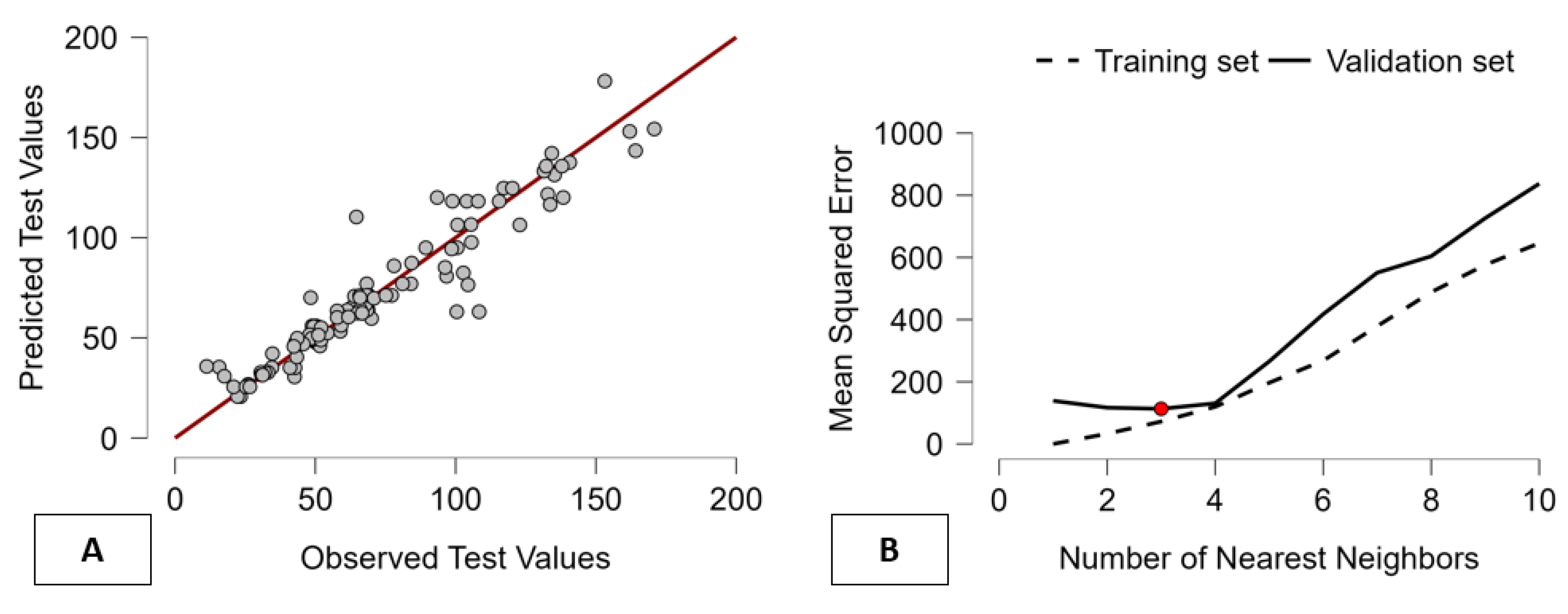
Figure 2.
Hierarchical Clustering Structure, Optimal Cluster Selection, and Environmental Regime Map.
Figure 2.
Hierarchical Clustering Structure, Optimal Cluster Selection, and Environmental Regime Map.
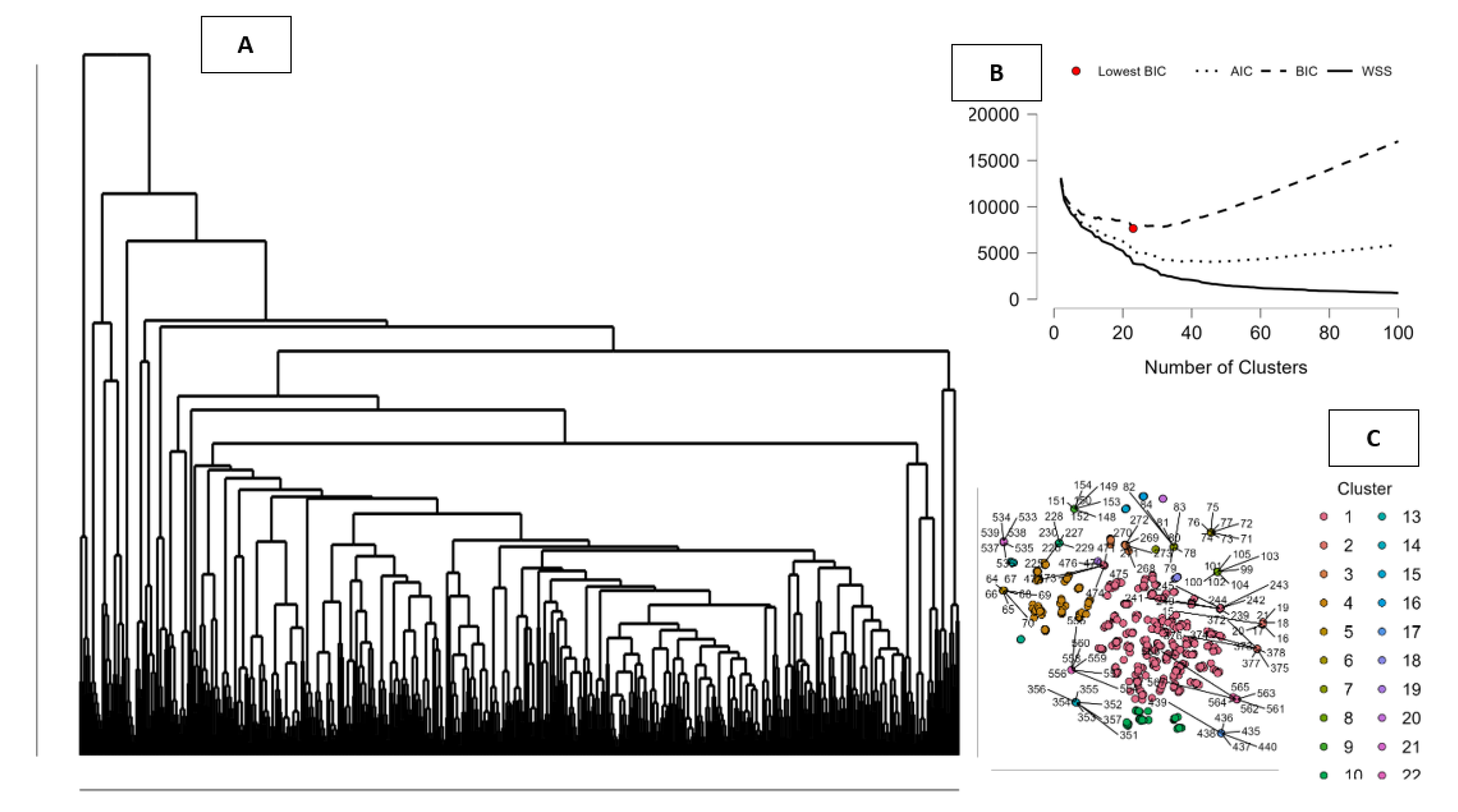
Figure 3.
Environmental–Financial Network Structure, Centrality Metrics, and Connectivity Measures.
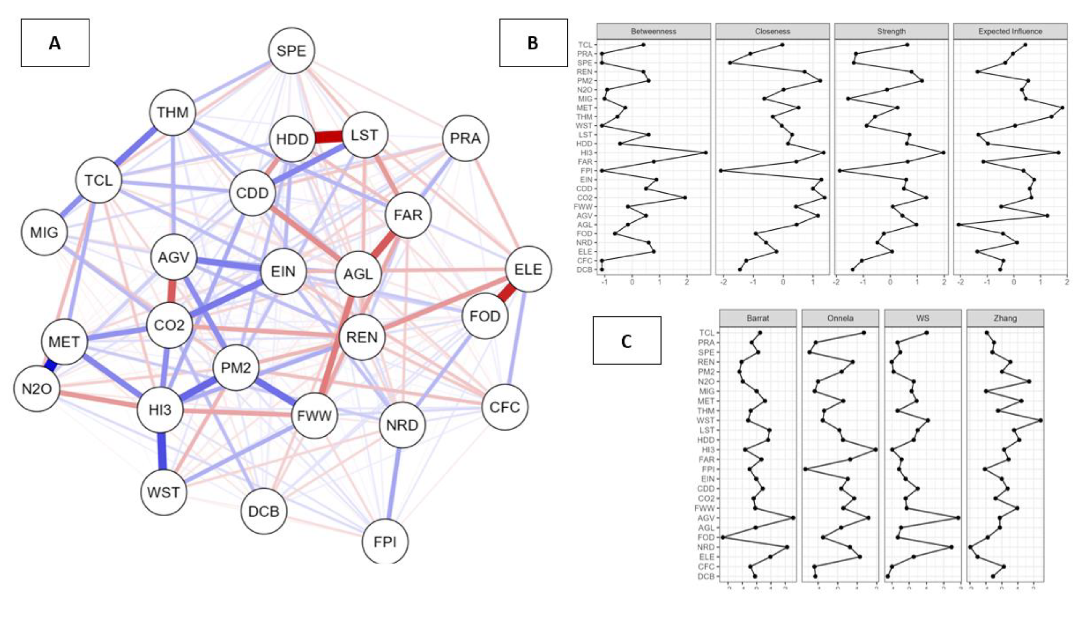
Figure 4.
Diagnostic Evaluation of the KNN Model for Predicting Domestic Credit to the Private Sector Using Social ESG Variables.
Figure 4.
Diagnostic Evaluation of the KNN Model for Predicting Domestic Credit to the Private Sector Using Social ESG Variables.
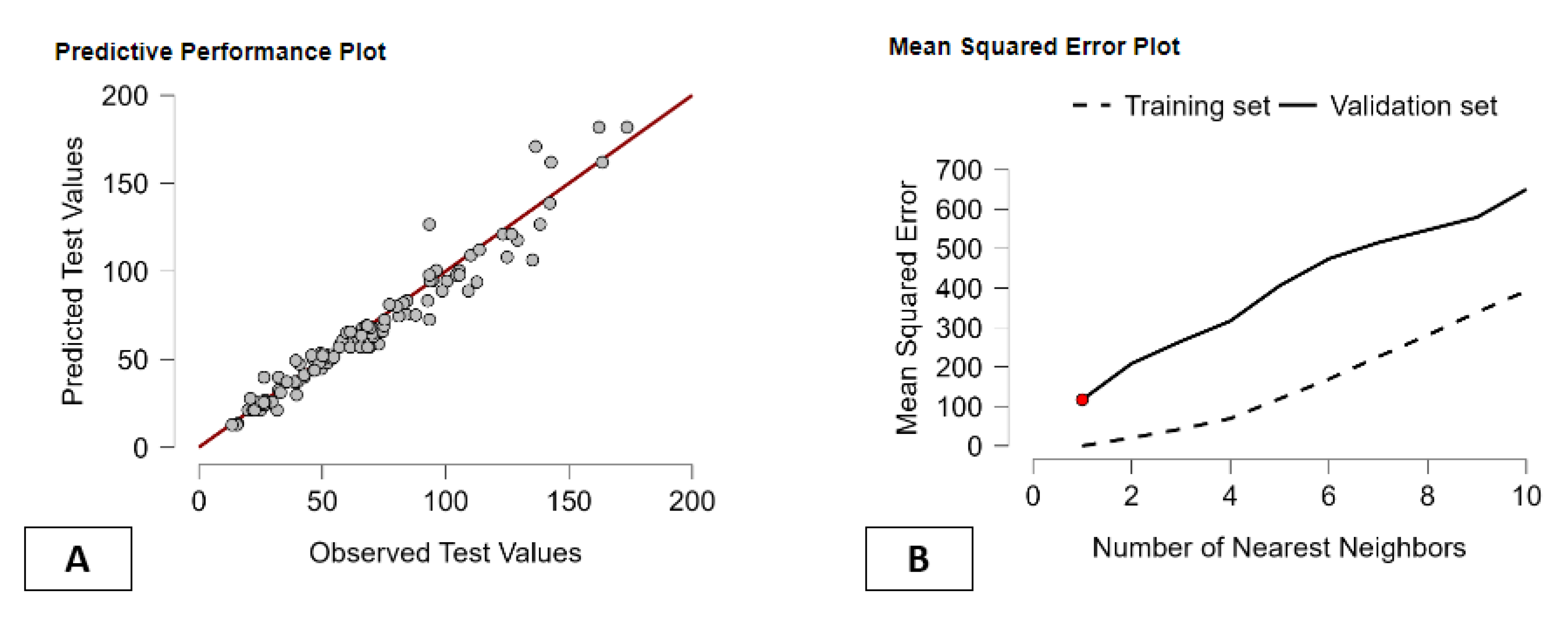
Figure 5.
Optimal Cluster Selection and Social Structure Visualization Using Fuzzy C-Means for the ESG Social Dimension.
Figure 5.
Optimal Cluster Selection and Social Structure Visualization Using Fuzzy C-Means for the ESG Social Dimension.
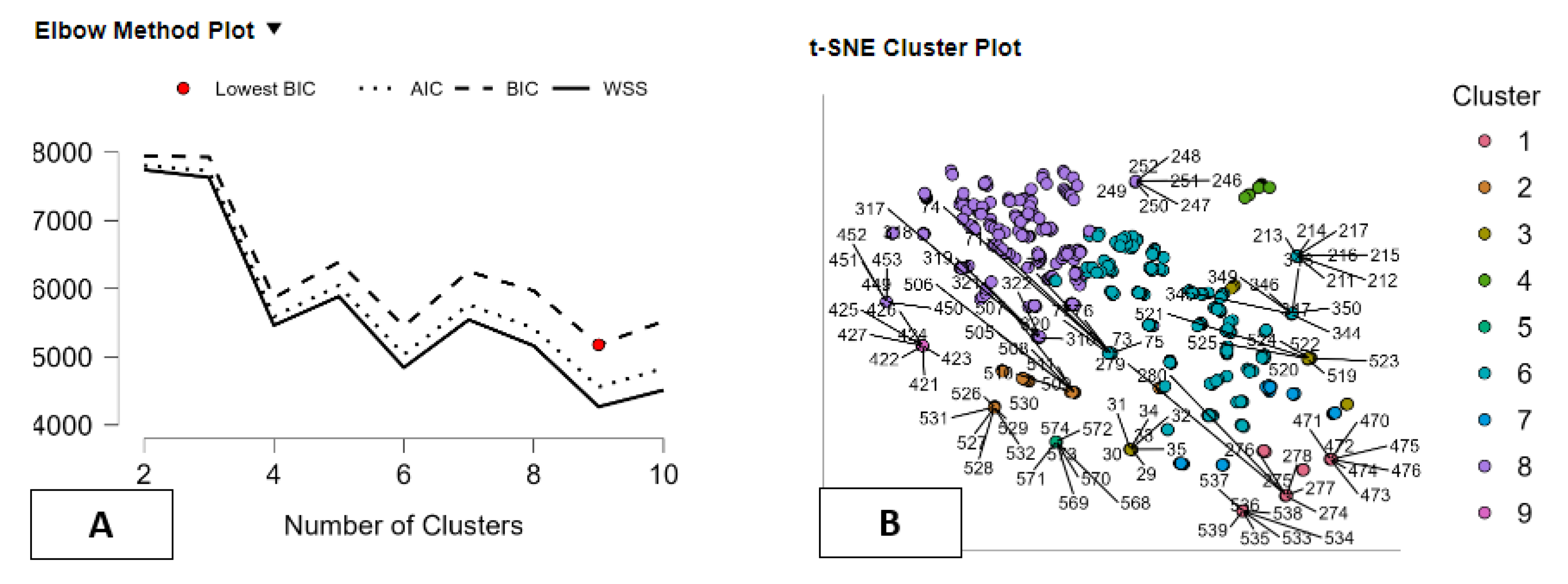
Figure 6.
Network Structure and Centrality Profiles of the Social (S) Dimension in the ESG Framework and Its Relationship with Domestic Credit (DCB).
Figure 6.
Network Structure and Centrality Profiles of the Social (S) Dimension in the ESG Framework and Its Relationship with Domestic Credit (DCB).
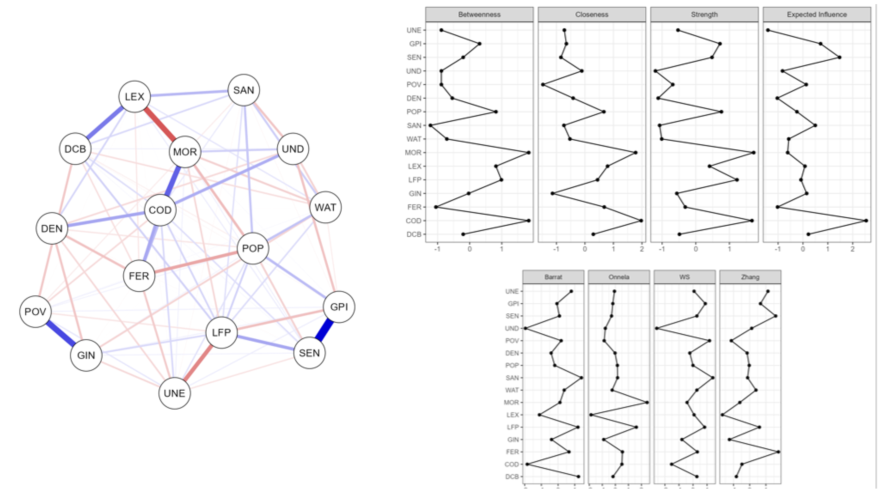
Figure 7.
Predictive Performance and Complexity Diagnostics of the Decision Tree Model for Governance-Based DCB Estimation.
Figure 7.
Predictive Performance and Complexity Diagnostics of the Decision Tree Model for Governance-Based DCB Estimation.
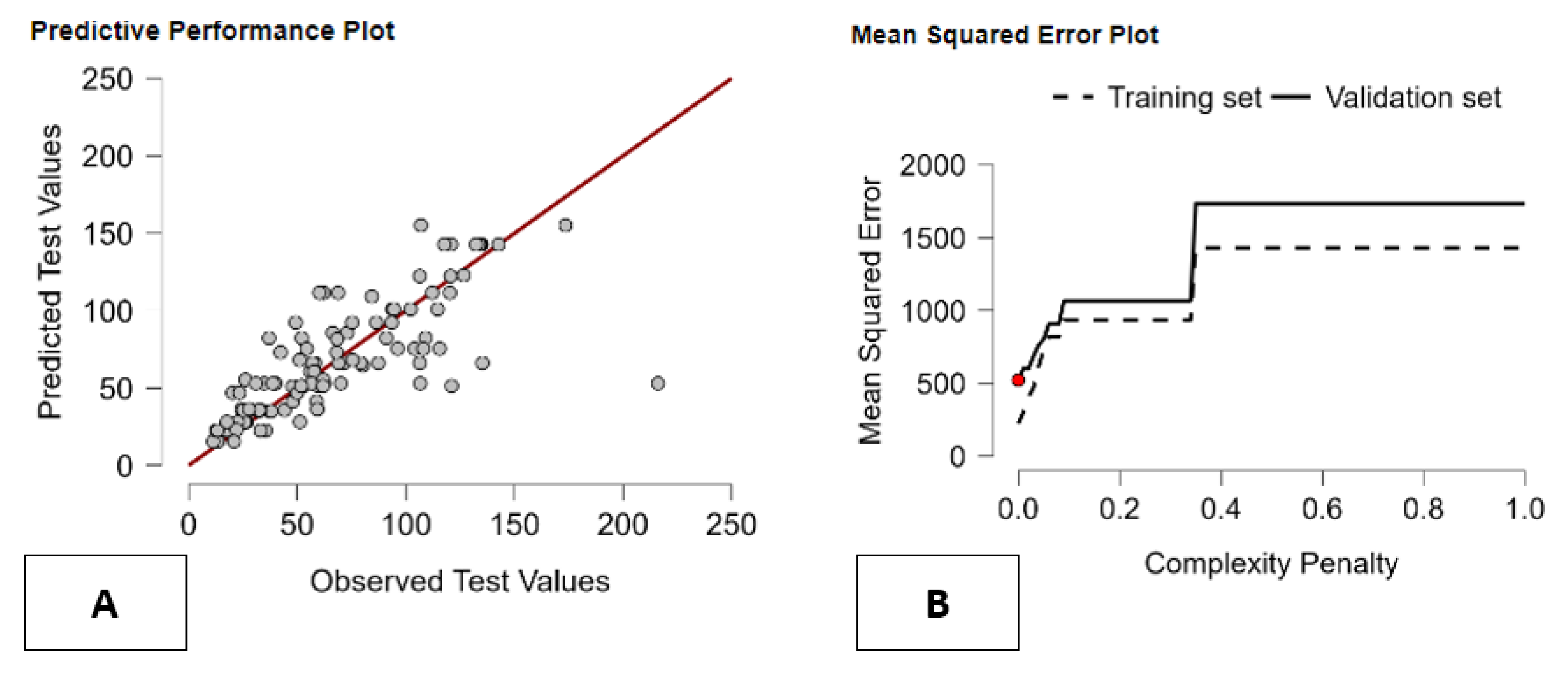
Figure 8.
Governance-Based Decision Tree for Predicting Domestic Credit to the Private Sector (DCB).
Figure 8.
Governance-Based Decision Tree for Predicting Domestic Credit to the Private Sector (DCB).
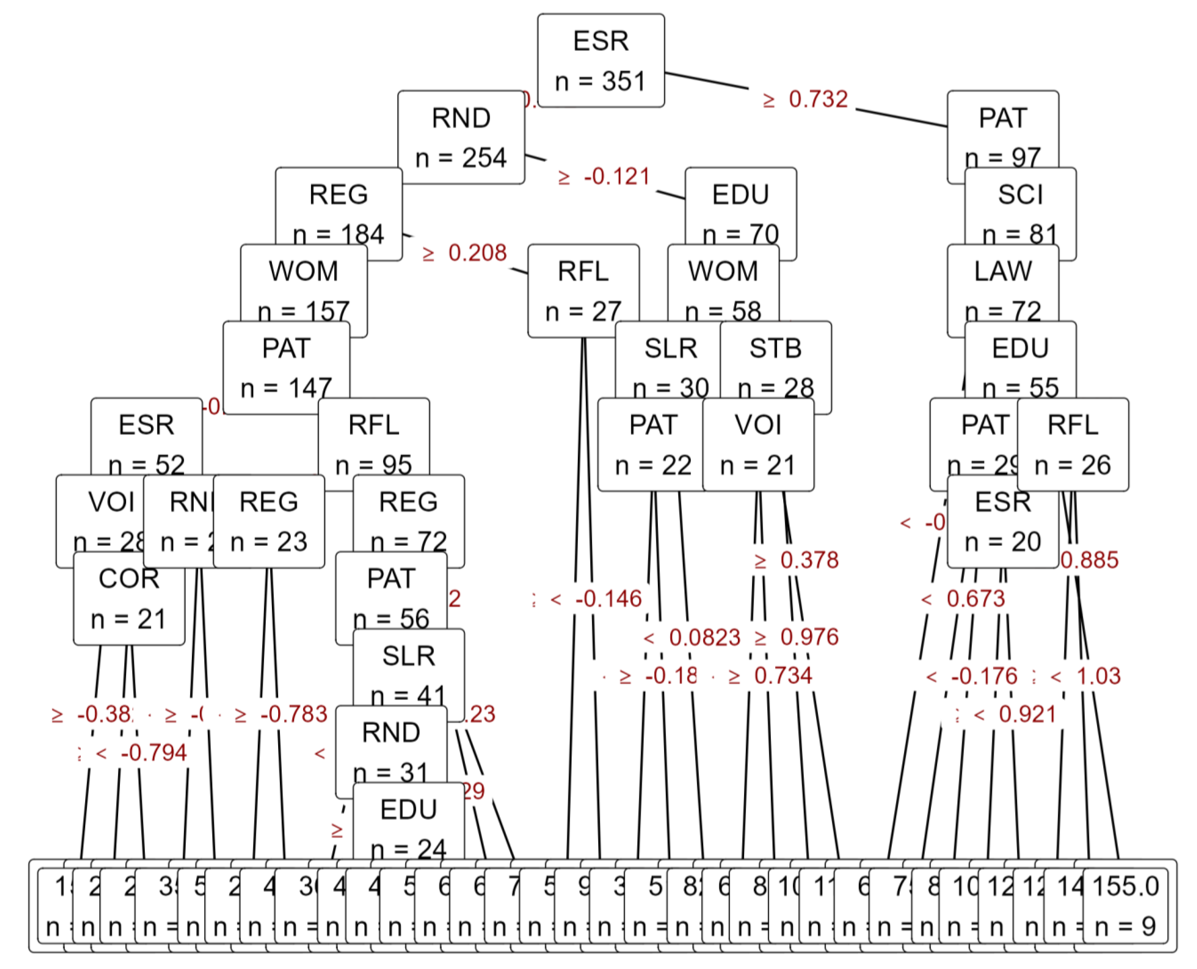
Figure 9.
Hierarchical Clustering Diagnostics for Governance-Based ESG Structures.
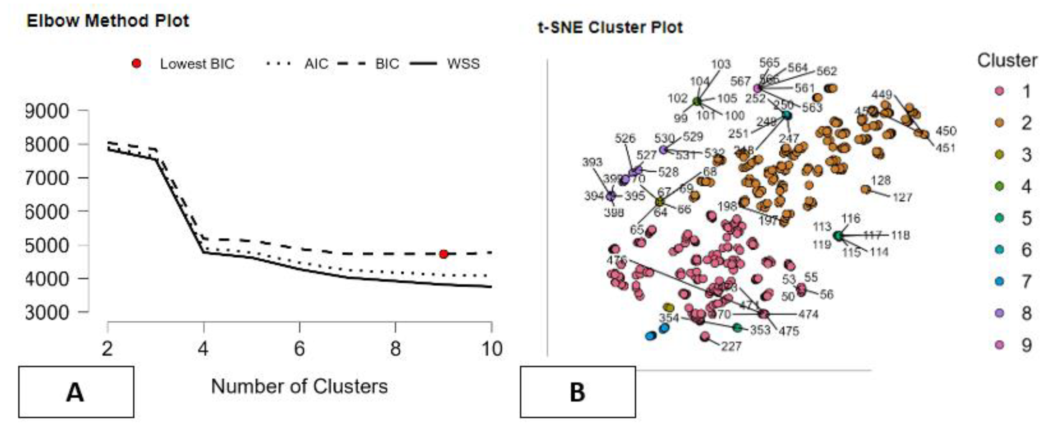
Figure 10.
Governance Network Structure and Centrality Profiles Under the ESG Framework.
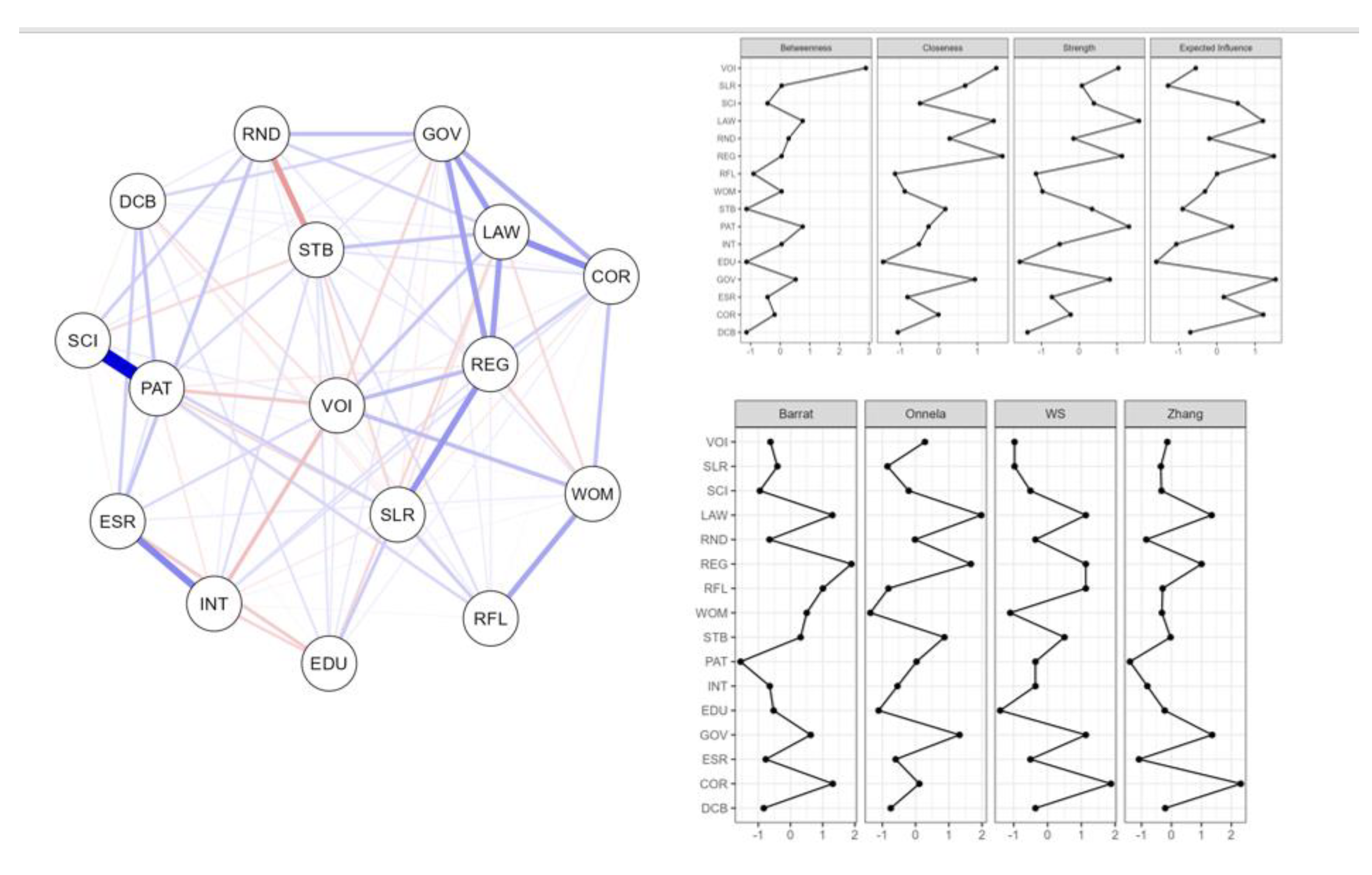
Table 1.
Comparative Summary of ESG Scholarship and Its Financial Implications.
| Macro-Theme | Articles Included | Methodologies Used | Main Findings |
| ESG Performance, Disclosure & Corporate Outcomes | Abdelfattah et al. (2025); Adebiyi et al. (2025); Alhassan et al.; Alvarez-Perez & Fuentes (2024); Capoani (2025); Laborda & Pérez (2025); Lotsu (2024); Malik & Sharma (2025); Parish (2025); Rashid & Aftab (2023); Wei et al. (2024); Zhao, Ngan & Jamil (2025); Zhao, Gao & Hong (2025); ΜAΓΚOΥΦH | Machine learning, firm-level econometrics, case studies, systematic reviews, panel regressions, supply-chain analysis | These papers study ESG performance or disclosure at firm or sectoral levels, showing links between ESG, financial performance, corporate risk, credit rating, or sustainability adoption. Many highlight the role of disclosure, private equity, corporate governance, and sustainability reporting. |
| ESG, Financial Development & Macro-Structural Dynamics | Acharya (2023); Aich et al. (2025); Alharbi (2024); Arnone et al. (2024); Chernykh et al. (2024); Guo & Naseer (2025); Hassani et al. (2024); Lamanda & Tamásné (2025); Lee et al. (2024); McHugh (2023); Mohamed (Egypt); Myronchuk et al. (2024); Subhani et al. (2025); Tan (2022); Trinh & Tran (2025); Xu et al. (2025) | Conceptual frameworks, macro-panel regressions, SEM, bibliometric analyses, policy analysis, case studies, credit-market analysis | These works connect ESG to macroeconomic outcomes—growth, financial depth, political stability, SDG financing, access to credit in specific regions. Often ESG is treated as dependent on financial development, institutional capacity, or inclusion. Others focus on policy instruments like green bonds or sovereign risk ratings. |
| Sustainable Finance Instruments, Markets & Regulation | Boström & Hannes (2024); Del Sarto & Ozili (2025); Kandpal et al. (2024); Pineau et al. (2022); Varney (2025); Wang & Zhao (2025); Shmatov & Castelli (2022); Soares (2024); Taušová et al. (2025); Yang et al. (2025) | Regulatory analysis, bibliometrics, policy evaluation, quantitative ESG metrics, credit rating models, market-level econometrics | Focus on green finance instruments (green bonds, sustainable financing frameworks), regulatory systems, FinTech, and how ESG shapes sovereign ratings, credit costs, or investment decisions. Strong emphasis on financial products and market structures. |
Table 2.
Instrumental Variables for the Estimation of DCB and the Environmental (E) Component of the ESG Framework.
Table 2.
Instrumental Variables for the Estimation of DCB and the Environmental (E) Component of the ESG Framework.
| Y | Domestic Credit to Private Sector by Banks | DCB |
| X | Access to clean fuels and technologies for cooking (% of population) | CFC |
| Adjusted savings: natural resources depletion (% of GNI) | ELE | |
| CO2 emissions (metric tons per capita) | CO2 | |
| Z | Economic and Social Rights Performance Score | ESR |
| GDP growth (annual %) | GDP | |
| Government expenditure on education, total (% of government expenditure) | EDU | |
| Patent applications, residents | PAT | |
| Regulatory Quality: Estimate | REG | |
| Rule of Law: Estimate | LAW | |
| Scientific and technical journal articles | SCI | |
| Individuals using the Internet (% of population) | INT | |
| Strength of legal rights index (0=weak to 12=strong) | SLR |
Table 3.
IV Estimation Results for Environmental Determinants of Domestic Credit (DCB).
| Statistic | CFC | ELE | CO2 | _cons |
| Coeff. (FD–IV) | 2.414805 | -1.533968 | -2.310756 | -0.9481893 |
| Coeff. (2SLS) | 1.383526 | -1.333478 | 1.207316 | 69.82275 |
| Coeff. (RE–IV) | 2.854203 | -3.860742 | -0.3478323 | 199.9138 |
| Std. Err (FD–IV) | 1.0422 | 1.248874 | 0.841417 | 0.4148102 |
| Std. Err (2SLS) | 0.206584 | 0.478682 | 0.390698 | 33.2518 |
| Std. Err (RE–IV) | 0.8635945 | 1.798736 | 0.6879378 | 119.8354 |
| z (FD–IV) | 2.32 | -1.23 | -2.75 | -2.29 |
| z (2SLS) | 6.70 | -2.79 | 3.09 | 2.10 |
| z (RE–IV) | 3.31 | -2.15 | -0.51 | 1.67 |
| P>|z| (FD–IV) | 0.021 | 0.219 | 0.006 | 0.022 |
| P>|z| (2SLS) | 0.000 | 0.005 | 0.002 | 0.036 |
| P>|z| (RE–IV) | 0.001 | 0.032 | 0.613 | 0.095 |
| 95% CI (FD–IV) | 0.3721–4.4575 | -3.9817–0.9138 | -3.9599–-0.6616 | -1.7612–-0.1352 |
| 95% CI (2SLS) | 0.9786–1.7884 | -2.2717–-0.3953 | 0.4416–1.9731 | 4.6504–134.9951 |
| 95% CI (RE–IV) | 1.1616–4.5468 | -7.3862–-0.3353 | -1.6962–1.0005 | -34.9593–434.7869 |
Table 4.
Comparative Model Diagnostics for FD–IV, 2SLS, and RE–IV Specifications.
| Category | Statistic / Info | FD–IV | 2SLS | RE–IV |
| Model type | Specification | First-Differenced Panel IV (FD–IV) | Instrumental Variable Regression (2SLS) | Random-Effects Panel IV (RE–IV) |
| Obs / Groups | Observations | 467 | 548 | 548 |
| Number of groups | 80 | — | 81 | |
| Fit / R2 | Within R2 | 0.0111 | — | 0.0040 |
| Between R2 | 0.1368 | — | 0.0167 | |
| Overall R2 | 0.0289 | Centered R2 = -0.1431, Uncentered R2 = 0.7276 | 0.0255 | |
| Root MSE | — | 41.42 | — | |
| Model tests | Wald χ2 / F | χ2(3) = 14.19, p = 0.0027 | F(3,544) = 37.44, p = 0.0000 | χ2(3) = 14.98, p = 0.0018 |
| corr(u_i, Xb) | -0.7209 | — | 0 (assumed) | |
| sigma_u | 59.779 | — | 42.0705 | |
| sigma_e | 16.396 | — | 9.9306 | |
| rho (intra-class corr.) | 0.930 | — | 0.9472 | |
| Identification tests | Underidentification | — | Anderson LM χ2(9) = 122.525, p = 0.0000 | — |
| Weak identification | — | Cragg-Donald F = 15.435 | — | |
| Overidentification | — | Sargan χ2(8) = 119.769, p = 0.0000 | — | |
| Endogenous vars. | cfc, ele | cfc, ele | cfc, ele | |
| Exogenous vars. | co2, esr, gdp, edu, pat, reg, rnd, law, sci, inst_int, slr | co2, esr, gdp, edu, pat, reg, rnd, law, sci, inst_int, slr | co2, esr, gdp, edu, pat, reg, rnd, law, sci, inst_int, slr | |
| Instruments | Included | — | co2 | — |
| Excluded | esr, gdp, edu, pat, reg, rnd, law, sci, inst_int, slr | esr, gdp, edu, pat, reg, rnd, law, sci, inst_int, slr | — | |
| Error structure | vce(cluster n) | Robust (clustered by n) | Homoskedastic (default) | Cluster-robust (by n) |
| Estimation note | Estimator | GMM (FD IV) | 2SLS IV (ivreghdfe) | G2SLS Random-Effects IV |
Table 5.
Robustness Checks Using IV–2SLS and FD–IV Estimators for Environmental Determinants of DCB.
Table 5.
Robustness Checks Using IV–2SLS and FD–IV Estimators for Environmental Determinants of DCB.
| Variables | (1) IV–2SLS (GMM2S, Cluster Robust) | (2) FD–IV (First-Difference, Cluster Robust) |
| Dependent variable: | dcb | D.dcb |
| cfc | 3.51 (2.51) | 2.41 (1.04)** |
| ele | -5.72 (5.59) | -1.53 (1.25) |
| co2 | 0.33 (1.22) | -2.31 (0.84)*** |
| Constant | 315.47 (335.81) | -0.95 (0.41)** |
| Observations | 548 | 467 |
| Clusters | 81 | 80 |
| F / Wald χ2 | 3.17 | 14.19 |
| Weak ID test (KP rk F) | 14.77 | — |
| Hansen J (p–value) | 0.337 | — |
| Underidentification test (p–value) | 0.0298 | — |
| Model type | Panel IV 2SLS (GMM2S + Fuller, cluster robust) | First-Difference IV (cluster robust) |
Table 6.
Environmental Variables Used for Modelling Domestic Credit to the Private Sector (DCB).
| Y | Domestic Credit to Private Sector by Banks | DCB |
| X | Agricultural land (% of land area) | AGL |
| Terrestrial and marine protected areas (% of total territorial area) | PRA | |
| Nitrous oxide emissions (metric tons of CO2 equivalent per capita) | N2O | |
| Forest area (% of land area) | FAR | |
| Methane emissions (metric tons of CO2 equivalent per capita) | MET | |
| Mammal species, threatened | THM | |
| PM2.5 air pollution, mean annual exposure (micrograms per cubic meter) | PM2 | |
| Renewable energy consumption (% of total final energy consumption) | REN | |
| Adjusted savings: natural resources depletion (% of GNI) | NRD | |
| Energy intensity level of primary energy (MJ/$2017 PPP GDP) | EIN | |
| Annual freshwater withdrawals, total (% of internal resources) | FWW | |
| Standardised Precipitation-Evapotranspiration Index | SPE | |
| Access to clean fuels and technologies for cooking (% of population) | CFC | |
| Food production index (2014-2016 = 100) | FPI | |
| Agriculture, forestry, and fishing, value added (% of GDP) | AGV | |
| CO2 emissions (metric tons per capita) | CO2 | |
| Access to electricity (% of population) | ELE | |
| Net migration | MIG | |
| Tree Cover Loss (hectares) | TCL | |
| Heating Degree Days | HDD | |
| Cooling Degree Days | CDD | |
| Adjusted savings: net forest depletion (% of GNI) | FOD | |
| Heat Index 35 | HI3 | |
| Land Surface Temperature | LST | |
| Level of water stress: freshwater withdrawal as a proportion of available freshwater resources | WST |
Table 7.
Comparative Predictive Performance of Machine-Learning Models for DCB Estimation.
| Model | MSE | MSE(scaled) | RMSE | MAE | MAPE | R2 |
| Boosting | 0.864 | 0.548 | 0.601 | 0.565 | 0.517 | 0.524 |
| Decision Tree | 0.461 | 0.164 | 0.317 | 0.277 | 0.276 | 0.811 |
| KNN | 0.131 | 0.000 | 0.000 | 0.000 | 0.000 | 1.000 |
| Linear Regression | 1.000 | 0.728 | 0.740 | 0.697 | 1.000 | 0.404 |
| ANN | 0.000 | 1.000 | 1.000 | 1.000 | 0.822 | 0.281 |
| Random Forest | 0.473 | 0.126 | 0.324 | 0.366 | 0.397 | 0.915 |
| Regularized Linear | 0.000 | 1.009 | 1.113 | 1.062 | 0.949 | 0.274 |
| SVM | 0.000 | 1.036 | 1.269 | 1.138 | 0.875 | 0.267 |
Table 8.
Mean Dropout Loss Values for Environmental ESG Variables in Predicting DCB.
| Variable | Mean dropout loss | Variable | Mean dropout loss |
| AGL | 15.496 | FPI | 10.758 |
| PRA | 15.442 | AGV | 10.736 |
| N2O | 14.527 | CO2 | 10.623 |
| FAR | 13.569 | ELE | 10.554 |
| MET | 12.815 | MIG | 10.482 |
| THM | 12.668 | TCL | 9.802 |
| PM2 | 12.393 | HDD | 9.594 |
| REN | 11.550 | CDD | 9.536 |
| NRD | 11.528 | FOD | 9.275 |
| EIN | 11.338 | HI3 | 9.255 |
| FWW | 11.300 | LST | 9.250 |
| SPE | 11.150 | WST | 8.820 |
| CFC | 10.882 |
Table 9.
Contribution of Environmental and Climate Variables to Predicted Domestic Credit Values.
| Case | Predicted | Base | CFC | ELE | NRD | FOD | AGL | AGV | FWW | CO2 | CDD | EIN | FPI |
| 1 | 35.410 | 68.222 | -0.725 | 0.114 | 0.541 | 0.533 | -0.771 | -4.416 | 0.530 | -0.391 | -6.326 | 6.087 | -4.273 |
| 2 | 35.754 | 68.222 | -1.427 | 0.189 | 0.493 | 0.143 | -1.027 | -4.538 | 0.512 | -0.192 | -1.462 | 2.121 | -0.469 |
| 3 | 55.972 | 68.222 | 0.894 | 0.394 | 0.725 | 0.352 | -7.782 | -4.163 | 0.482 | 0.139 | -1.324 | 0.650 | 2.786 |
| 4 | 53.257 | 68.222 | 0.417 | 0.342 | 0.402 | 0.550 | -1.818 | -5.763 | 0.507 | -0.441 | -1.504 | 1.297 | 5.070 |
| 5 | 55.972 | 68.222 | 0.192 | 0.419 | 0.455 | 0.828 | -1.818 | -5.987 | 0.530 | -1.267 | -1.169 | 0.356 | 10.888 |
| FAR | HI3 | HDD | LST | WST | THM | MET | MIG | N2O | PM2 | REN | SPE | PRA | TCL |
| -4.244 | -1.214 | 0.229 | -2.683 | -0.602 | 0.327 | -6.170 | -1.252 | -10.183 | 0.788 | -3.276 | 3.759 | 1.445 | -0.640 |
| -6.566 | -1.515 | 0.506 | 0.875 | -0.443 | -0.467 | -7.233 | -0.376 | -8.955 | 1.059 | -3.333 | -1.576 | 1.781 | -0.568 |
| 1.651 | -0.554 | -1.477 | -1.661 | 0.034 | -3.172 | -1.417 | 0.041 | 1.505 | 2.627 | 0.174 | 1.266 | -3.947 | -0.475 |
| 2.667 | -0.544 | -0.835 | -1.985 | -0.081 | -3.618 | -1.755 | 0.008 | 1.035 | -1.617 | 1.155 | -2.090 | -5.907 | -0.457 |
| 2.849 | -0.238 | -0.099 | -7.343 | -0.257 | -3.889 | -1.775 | -0.543 | 0.961 | -1.746 | 1.843 | 0.428 | -5.346 | -0.523 |
Table 10.
Comparative Clustering Performance for Environmental Determinants of Domestic Credit (DCB).
Table 10.
Comparative Clustering Performance for Environmental Determinants of Domestic Credit (DCB).
| Statistics | K-Means | Density-Based | Hierarchical | Model-Based | Random Forest | Fuzzy C-Means |
| R2 | 0.693 | 0.865 | 0.727 | 0.772 | 0.609 | 0.433 |
| AIC | 5.244 | 3.526 | 5.075 | 4.808 | 6.648 | 9.745 |
| BIC | 7.147 | 8.340 | 7.650 | 8.167 | 8.999 | 10.753 |
| Silhouette | 0.220 | 0.290 | 0.300 | 0.240 | 0.160 | 0.010 |
| Maximum diameter | 9.347 | 21.738 | 7.751 | 11.758 | 16.678 | 18.743 |
| Minimum separation | 0.780 | 1.570 | 2.233 | 0.857 | 1.168 | 0.251 |
| Pearson's γ | 0.352 | 0.268 | 0.548 | 0.256 | 0.250 | 0.199 |
| Dunn index | 0.083 | 0.072 | 0.288 | 0.073 | 0.070 | 0.013 |
| Entropy | 2.398 | 3.174 | 1.930 | 2.945 | 2.900 | 2.050 |
| Calinski-Harabasz index | 75.057 | 19.975 | 63.625 | 60.347 | 41.097 | 35.904 |
Table 11.
Hierarchical Clustering Structure and Cohesion Metrics for Environmental Determinants of DCB.
Table 11.
Hierarchical Clustering Structure and Cohesion Metrics for Environmental Determinants of DCB.
| Cluster | 1 | 2 | 3 | 4 | 5 | 6 | 7 | 8 | 9 | 10 | 11 | 12 |
| Size | 286 | 14 | 14 | 81 | 7 | 7 | 9 | 7 | 7 | 35 | 6 | 7 |
| Explained proportion within-cluster heterogeneity | 0.643 | 0.027 | 0.017 | 0.172 | 0.001 | 0.003 | 0.009 | 0.002 | 0.001 | 0.062 | 0.006 | 0.003 |
| Within sum of squares | 2.492 | 106.483 | 67.319 | 669.067 | 5.369 | 12.809 | 34.785 | 6.926 | 5.593 | 238.884 | 21.907 | 11.934 |
| Silhouette score | 0.141 | 0.401 | 0.488 | 0.204 | 0.761 | 0.721 | 0.552 | 0.753 | 0.884 | 0.346 | 0.595 | 0.714 |
| Cluster | 13 | 14 | 15 | 16 | 17 | 18 | 19 | 20 | 21 | 22 | 23 | |
| Size | 7 | 7 | 7 | 7 | 6 | 5 | 1 | 7 | 7 | 7 | 7 | |
| Explained proportion within-cluster heterogeneity | 0.005 | 0.008 | 0.005 | 0.010 | 0.004 | 0.002 | 0.000 | 0.001 | 0.011 | 0.002 | 0.005 | |
| Within sum of squares | 18.227 | 31.087 | 20.880 | 37.602 | 15.525 | 7.942 | 0.000 | 4.886 | 41.838 | 7.325 | 19.851 | |
| Silhouette score | 0.648 | 0.628 | 0.681 | 0.603 | 0.715 | 0.675 | 0.000 | 0.859 | 0.639 | 0.773 | 0.700 |
Table 12.
Environmental–Economic Cluster Means for DCB: Multidimensional Profiles Across 23 Country Groups.
Table 12.
Environmental–Economic Cluster Means for DCB: Multidimensional Profiles Across 23 Country Groups.
| Cluster Means | |||||||||||||
| DCB | CFC | ELE | NRD | FOD | AGL | AGV | FWW | CO2 | CDD | EIN | FPI | FAR | |
| Cluster 1 | 0.254 | -0.283 | -0.550 | 0.347 | -0.079 | -0.063 | -0.283 | 0.226 | -0.169 | -0.147 | -0.237 | -0.138 | 0.274 |
| Cluster 2 | 0.076 | -0.247 | 0.028 | 0.505 | 1.060 | 1.830 | 0.145 | 0.263 | -0.181 | -0.158 | -0.424 | -0.167 | -0.292 |
| Cluster 3 | 1.377 | -0.008 | -0.345 | 0.317 | 0.296 | -1.185 | 0.789 | 0.263 | -1.250 | -0.174 | 0.934 | -0.061 | 0.680 |
| Cluster 4 | -0.184 | 0.624 | 1.084 | -0.441 | -0.701 | -0.119 | -0.377 | -0.005 | 0.881 | -0.013 | 0.089 | -0.157 | -1.086 |
| Cluster 5 | 0.204 | -0.693 | 0.706 | -1.061 | -0.634 | -0.899 | -0.488 | -3.212 | -0.193 | 0.121 | -0.556 | -0.160 | -1.082 |
| Cluster 6 | -0.668 | 0.043 | 1.474 | 0.336 | -0.793 | -0.118 | 0.015 | 0.229 | 1.532 | -0.174 | 0.322 | -0.169 | -1.201 |
| Cluster 7 | 0.460 | -0.346 | -0.515 | -3.895 | -0.109 | -0.217 | 0.363 | 0.154 | -0.002 | -0.174 | -0.010 | -0.137 | 0.169 |
| Cluster 8 | 0.708 | 0.460 | -0.469 | -0.448 | 0.301 | 2.476 | 1.457 | 0.263 | -0.411 | -0.174 | -0.051 | -0.145 | 1.331 |
| Cluster 9 | -1.914 | 1.241 | 1.201 | 0.501 | -0.766 | -1.097 | -0.367 | 0.263 | -1.640 | -0.006 | -0.369 | 8.539 | -0.970 |
| Cluster 10 | -1.631 | -0.756 | -0.744 | 0.505 | 0.370 | 1.393 | 0.187 | 0.263 | 1.645 | -0.174 | -0.517 | -0.154 | 1.237 |
| Cluster 11 | 0.944 | 2.473 | 1.606 | -1.192 | -0.872 | -0.481 | 0.240 | -0.320 | -0.358 | 0.003 | 0.946 | -0.118 | -0.941 |
| Cluster 12 | -0.403 | 1.655 | 1.524 | -0.397 | -0.800 | -0.952 | -0.459 | 0.062 | 0.995 | -0.174 | 0.568 | -0.157 | -1.217 |
| Cluster 13 | 0.358 | 3.343 | 1.578 | -3.075 | -1.138 | -0.957 | 0.786 | -3.733 | -1.306 | 1.361 | -0.302 | -0.147 | -1.197 |
| Cluster 14 | 1.578 | 1.492 | -0.755 | -1.732 | 0.116 | -0.537 | 1.463 | -0.095 | -1.158 | -0.174 | 2.285 | -0.168 | 2.354 |
| Cluster 15 | -1.874 | -0.679 | 2.407 | 0.505 | 2.069 | -0.095 | 1.647 | 0.263 | -1.642 | -0.172 | 2.560 | -0.034 | -1.219 |
| Cluster 16 | -1.789 | -1.055 | 2.397 | 0.505 | 5.338 | 0.801 | 1.667 | 0.263 | -1.642 | -0.174 | 2.933 | 0.352 | -1.192 |
| Cluster 17 | -1.444 | -0.327 | -0.905 | -0.386 | 1.083 | -0.397 | 2.530 | 0.246 | 1.008 | -0.174 | 0.346 | -0.168 | 3.156 |
| Cluster 18 | -2.066 | -1.102 | 2.133 | 0.505 | 0.416 | 1.363 | -0.830 | 0.263 | -0.454 | -0.174 | 1.475 | -0.073 | -1.227 |
| Cluster 19 | 1.920 | -0.598 | -0.048 | -0.168 | 0.320 | -0.213 | 1.932 | -1.556 | -0.888 | -0.174 | -0.799 | -0.120 | -0.756 |
| Cluster 20 | -1.836 | -0.938 | 2.604 | 0.505 | 2.976 | 0.185 | 0.829 | 0.263 | -1.404 | -0.174 | 0.917 | 1.744 | -1.205 |
| Cluster 21 | 1.537 | 3.848 | 0.808 | -3.861 | -1.190 | -1.456 | 4.426 | -6.714 | -1.005 | 8.287 | 0.700 | -0.168 | -1.225 |
| Cluster 22 | 1.994 | 0.285 | -0.293 | 0.505 | -0.831 | -1.120 | -0.712 | 0.248 | -1.034 | -0.174 | -0.721 | -0.165 | -0.691 |
| Cluster 23 | 0.139 | -0.913 | -0.373 | 0.505 | 1.753 | -0.448 | 0.322 | 0.263 | 0.161 | -0.174 | -0.113 | -0.152 | 0.814 |
| HI3 | HDD | LST | WST | THM | MET | MIG | N2O | PM2 | REN | SPE | PRA | TCL | |
| Cluster 1 | -0.287 | -0.321 | -0.303 | -0.070 | -0.109 | -0.400 | -0.289 | 0.198 | -0.189 | -0.134 | -0.261 | -0.418 | -0.145 |
| Cluster 2 | -0.096 | 0.295 | 2.572 | 0.576 | 3.099 | -0.094 | -1.032 | 1.273 | -0.122 | 0.250 | 0.323 | 0.526 | -0.248 |
| Cluster 3 | -0.259 | -0.151 | 0.595 | -0.268 | -0.170 | 3.007 | 0.105 | -0.842 | -1.104 | -0.469 | -0.304 | -0.293 | -0.052 |
| Cluster 4 | 0.129 | 0.742 | -0.286 | -0.009 | -0.421 | 0.024 | 0.112 | -0.243 | 0.370 | 0.133 | -0.028 | 0.689 | -0.187 |
| Cluster 5 | -0.296 | 1.303 | -0.224 | -0.193 | 0.436 | -0.309 | 0.258 | 1.159 | 0.254 | -0.031 | -0.305 | -0.327 | -0.270 |
| Cluster 6 | -0.265 | 0.767 | 0.286 | 0.167 | 0.289 | 0.022 | -0.669 | 1.037 | 1.434 | -1.149 | 4.562 | 2.026 | -0.270 |
| Cluster 7 | -0.296 | -0.064 | -0.384 | -0.556 | -0.201 | -0.436 | 0.033 | 0.741 | -0.329 | -0.025 | -0.298 | -0.414 | -0.045 |
| Cluster 8 | -0.092 | -0.294 | -0.425 | -1.319 | -0.377 | -0.279 | 1.968 | -0.085 | -0.438 | 0.672 | 0.451 | 1.787 | -0.051 |
| Cluster 9 | -0.167 | 1.596 | -0.525 | -0.370 | -0.629 | 0.575 | 3.232 | -0.375 | -0.894 | -1.005 | -0.305 | -0.088 | 0.436 |
| Cluster 10 | -0.256 | -1.499 | -0.563 | 0.198 | -0.167 | -0.192 | -0.660 | -0.482 | 0.683 | 0.751 | -0.109 | -0.347 | -0.139 |
| Cluster 11 | 2.353 | 1.164 | -0.597 | -1.740 | -0.654 | -0.217 | 4.429 | -1.065 | 0.670 | 0.874 | -0.107 | 2.469 | 0.072 |
| Cluster 12 | -0.227 | 0.639 | -0.192 | -0.419 | -0.548 | 0.079 | -0.122 | -0.925 | 0.092 | 1.087 | 1.462 | 5.810 | -0.123 |
| Cluster 13 | -0.148 | 1.614 | -0.500 | -0.549 | -0.393 | 0.040 | 0.192 | -0.467 | 2.803 | 1.595 | -0.283 | 0.321 | -0.105 |
| Cluster 14 | -0.296 | -0.779 | 2.230 | -0.164 | 5.403 | 1.871 | 1.145 | 0.237 | -1.014 | -0.556 | -0.295 | -0.327 | -0.263 |
| Cluster 15 | 2.743 | 2.256 | 1.524 | -0.462 | -0.602 | 5.234 | 1.582 | -1.280 | -1.205 | -1.307 | -0.305 | -0.361 | 0.338 |
| Cluster 16 | 5.714 | 1.876 | 5.341 | -0.176 | -0.611 | 1.439 | 3.883 | -0.977 | -1.203 | -0.902 | -0.305 | -0.566 | 2.008 |
| Cluster 17 | -0.296 | -2.638 | 1.445 | 1.767 | -0.280 | 1.461 | -0.661 | -0.704 | -1.019 | -0.057 | 6.730 | 0.457 | -0.259 |
| Cluster 18 | -0.231 | 1.283 | -0.471 | -0.017 | 1.473 | -0.498 | -0.198 | -1.166 | -1.161 | -0.044 | -0.305 | -0.225 | 0.159 |
| Cluster 19 | -0.295 | 0.993 | -0.162 | -5.147 | -0.480 | -0.050 | 0.524 | -0.250 | -0.760 | -1.132 | -0.206 | 0.321 | 0.043 |
| Cluster 20 | 4.896 | 2.340 | 2.513 | -0.259 | -0.631 | 0.832 | 1.564 | -0.109 | -1.181 | -1.178 | -0.305 | -0.429 | 8.414 |
| Cluster 21 | -0.296 | 0.889 | -0.611 | 0.277 | -0.523 | 2.479 | 1.161 | 0.019 | 3.946 | 1.692 | -0.203 | 0.355 | -0.250 |
| Cluster 22 | -0.294 | 0.278 | 2.512 | -0.226 | 2.373 | -0.495 | -0.807 | -1.176 | 2.183 | 0.042 | -0.280 | -0.361 | -0.229 |
| Cluster 23 | -0.241 | -0.473 | 0.359 | 6.472 | 0.215 | -0.422 | -0.944 | 0.624 | -0.633 | 1.184 | 2.547 | 0.662 | -0.131 |
Table 13.
Network Connectivity Measures for Environmental, Energy, and Resource Variables.
| Number of nodes | Number of non-zero edges | Sparsity |
| 26 | 257 / 325 | 0.209 |
Table 14.
Centrality Measures of Environmental, Climate, and Energy Variables in the DCB Network.
| Centrality measures per variable | ||||
| Network | ||||
| Variable | Betweenness | Closeness | Strength | Expected influence |
| AGL | -0.157 | 0.449 | 0.967 | -2.075 |
| AGV | 0.506 | 1.167 | 0.447 | 1.259 |
| CDD | 0.506 | 0.996 | 0.507 | 0.596 |
| CFC | -1.103 | -1.241 | -1.055 | -0.397 |
| CO2 | 1.925 | 1.392 | 1.330 | 0.658 |
| DCB | -1.103 | -1.453 | -1.394 | -0.512 |
| EIN | 0.884 | 1.281 | 0.587 | 0.761 |
| ELE | 0.790 | -0.226 | 0.065 | -1.375 |
| FAR | 0.790 | 0.439 | 0.644 | -1.146 |
| FOD | -0.630 | -0.919 | -0.240 | -0.409 |
| FPI | -1.103 | -2.095 | -1.874 | 0.359 |
| FWW | -0.157 | 0.430 | 0.088 | -0.477 |
| HDD | -0.440 | 0.162 | 0.616 | -0.977 |
| HI3 | 2.682 | 1.358 | 1.972 | 1.676 |
| LST | 0.601 | 0.301 | 0.710 | -1.333 |
| MET | -0.251 | 0.515 | 0.265 | 1.821 |
| MIG | -1.008 | -0.636 | -1.560 | 0.447 |
| N2O | -0.914 | 0.012 | -0.122 | 0.303 |
| NRD | 0.601 | -0.576 | -0.480 | 0.118 |
| PM2 | 0.601 | 1.242 | 1.172 | 0.538 |
| PRA | -1.103 | -1.103 | -1.271 | -0.033 |
| REN | 0.411 | 0.718 | 0.788 | -1.365 |
| SPE | -1.103 | -1.786 | -1.352 | -0.321 |
| TCL | 0.411 | -0.027 | 0.630 | 0.430 |
| THM | -0.535 | -0.352 | -0.565 | 1.411 |
| WST | -1.103 | -0.049 | -0.877 | 0.043 |
Table 15.
Weighted Adjacency Matrix of the Environmental–Financial Interaction Network.
| Weights matrix Network | |||||||||||||
| Variable | DCB | CFC | ELE | NRD | FOD | AGL | AGV | FWW | CO2 | CDD | EIN | FPI | FAR |
| DCB | 0.000 | 0.184 | -0.306 | -0.106 | -0.115 | -0.132 | 0.011 | 0.000 | -0.441 | 0.006 | 0.000 | -0.346 | -0.096 |
| CFC | 0.184 | 0.000 | 0.121 | -0.016 | -0.437 | -0.064 | 0.345 | 0.000 | 0.000 | 0.101 | 0.023 | 0.042 | 0.021 |
| ELE | -0.306 | 0.121 | 0.000 | -0.065 | 0.000 | 0.040 | 0.000 | 0.000 | 0.063 | -0.015 | 0.025 | 0.000 | -0.279 |
| NRD | -0.106 | -0.016 | -0.065 | 0.000 | 0.027 | 0.042 | -0.153 | 0.198 | -0.019 | 0.040 | -0.047 | 0.103 | 0.000 |
| FOD | -0.115 | -0.437 | 0.000 | 0.027 | 0.000 | 0.177 | 0.362 | 0.000 | -0.069 | 0.043 | 0.066 | -0.022 | 0.079 |
| AGL | -0.132 | -0.064 | 0.040 | 0.042 | 0.177 | 0.000 | -0.038 | 0.072 | 0.000 | 0.072 | -0.091 | -0.108 | -0.002 |
| AGV | 0.011 | 0.345 | 0.000 | -0.153 | 0.362 | -0.038 | 0.000 | -0.190 | 0.083 | 0.147 | 0.012 | -0.032 | 0.188 |
| FWW | 0.000 | 0.000 | 0.000 | 0.198 | 0.000 | 0.072 | -0.190 | 0.000 | 0.102 | -0.587 | 0.062 | 0.047 | 0.000 |
| CO2 | -0.441 | 0.000 | 0.063 | -0.019 | -0.069 | 0.000 | 0.083 | 0.102 | 0.000 | -0.016 | 0.000 | -0.229 | -0.167 |
| CDD | 0.006 | 0.101 | -0.015 | 0.040 | 0.043 | 0.072 | 0.147 | -0.587 | -0.016 | 0.000 | -0.023 | 0.000 | -0.090 |
| EIN | 0.000 | 0.023 | 0.025 | -0.047 | 0.066 | -0.091 | 0.012 | 0.062 | 0.000 | -0.023 | 0.000 | -0.098 | 0.024 |
| FPI | -0.346 | 0.042 | 0.000 | 0.103 | -0.022 | -0.108 | -0.032 | 0.047 | -0.229 | 0.000 | -0.098 | 0.000 | 0.000 |
| FAR | -0.096 | 0.021 | -0.279 | 0.000 | 0.079 | -0.002 | 0.188 | 0.000 | -0.167 | -0.090 | 0.024 | 0.000 | 0.000 |
| HI3 | -0.028 | 0.000 | 0.224 | 0.068 | 0.305 | 0.012 | 0.000 | 0.075 | 0.000 | -0.056 | 0.074 | -0.243 | 0.005 |
| HDD | 0.043 | 0.000 | 0.328 | -0.006 | 0.000 | -0.018 | 0.000 | -0.141 | -0.270 | -0.066 | 0.041 | 0.022 | -0.682 |
| LST | 0.077 | 0.000 | 0.000 | 0.037 | 0.291 | -0.062 | 0.000 | 0.012 | -0.102 | -0.045 | 0.000 | 0.000 | -0.029 |
| WST | -9.030×10⁻⁴ | 0.000 | 0.004 | 0.064 | 0.183 | -0.046 | -0.077 | -0.008 | 0.014 | 0.109 | -0.027 | 0.064 | 0.000 |
| THM | 0.015 | 0.128 | 0.046 | -0.003 | -0.059 | 0.042 | -0.003 | 0.000 | 0.000 | -0.043 | 0.097 | 0.014 | 0.108 |
| MET | -0.097 | 0.000 | 0.134 | 0.077 | -0.021 | -0.104 | 0.167 | 0.000 | -0.127 | 0.193 | 0.238 | 0.000 | 0.092 |
| MIG | 0.000 | 0.305 | -0.010 | -0.167 | 0.000 | 0.000 | 0.052 | 0.000 | -0.003 | -0.003 | 0.078 | 0.384 | 0.170 |
| N2O | 0.115 | -0.046 | -0.146 | 0.043 | 0.104 | 0.023 | -0.115 | -0.163 | 0.199 | 0.000 | -0.017 | 0.072 | 0.000 |
| PM2 | -0.124 | 0.172 | 0.031 | -0.146 | -0.239 | 0.000 | -0.090 | -0.276 | 0.133 | 0.088 | -0.003 | 0.000 | -0.064 |
| REN | -0.004 | 0.044 | 0.070 | -0.050 | 0.040 | 0.050 | -0.036 | -0.076 | 0.022 | 0.059 | 0.058 | -0.011 | -0.008 |
| SPE | -0.080 | 0.000 | 0.195 | -0.025 | -0.027 | -0.067 | 0.172 | 0.000 | 0.039 | -0.070 | 0.000 | 0.000 | 0.150 |
| PRA | 0.136 | 0.203 | 0.177 | 0.027 | -0.003 | 0.072 | -0.045 | 0.063 | 0.196 | 0.000 | 0.012 | -0.027 | -0.008 |
| TCL | -0.035 | 0.000 | 0.003 | -0.014 | 0.000 | -0.046 | 0.000 | 0.000 | -0.050 | 0.056 | -0.039 | 0.218 | 0.071 |
| HI3 | HDD | LST | WST | THM | MET | MIG | N2O | PM2 | REN | SPE | PRA | TCL | |
| DCB | -0.028 | 0.043 | 0.077 | -9.030×10⁻⁴ | 0.015 | -0.097 | 0.000 | 0.115 | -0.124 | -0.004 | -0.080 | 0.136 | -0.035 |
| CFC | 0.000 | 0.000 | 0.000 | 0.000 | 0.128 | 0.000 | 0.305 | -0.046 | 0.172 | 0.044 | 0.000 | 0.203 | 0.000 |
| ELE | 0.224 | 0.328 | 0.000 | 0.004 | 0.046 | 0.134 | -0.010 | -0.146 | 0.031 | 0.070 | 0.195 | 0.177 | 0.003 |
| NRD | 0.068 | -0.006 | 0.037 | 0.064 | -0.003 | 0.077 | -0.167 | 0.043 | -0.146 | -0.050 | -0.025 | 0.027 | -0.014 |
| FOD | 0.305 | 0.000 | 0.291 | 0.183 | -0.059 | -0.021 | 0.000 | 0.104 | -0.239 | 0.040 | -0.027 | -0.003 | 0.000 |
| AGL | 0.012 | -0.018 | -0.062 | -0.046 | 0.042 | -0.104 | 0.000 | 0.023 | 0.000 | 0.050 | -0.067 | 0.072 | -0.046 |
| AGV | 0.000 | 0.000 | 0.000 | -0.077 | -0.003 | 0.167 | 0.052 | -0.115 | -0.090 | -0.036 | 0.172 | -0.045 | 0.000 |
| FWW | 0.075 | -0.141 | 0.012 | -0.008 | 0.000 | 0.000 | 0.000 | -0.163 | -0.276 | -0.076 | 0.000 | 0.063 | 0.000 |
| CO2 | 0.000 | -0.270 | -0.102 | 0.014 | 0.000 | -0.127 | -0.003 | 0.199 | 0.133 | 0.022 | 0.039 | 0.196 | -0.050 |
| CDD | -0.056 | -0.066 | -0.045 | 0.109 | -0.043 | 0.193 | -0.003 | 0.000 | 0.088 | 0.059 | -0.070 | 0.000 | 0.056 |
| EIN | 0.074 | 0.041 | 0.000 | -0.027 | 0.097 | 0.238 | 0.078 | -0.017 | -0.003 | 0.058 | 0.000 | 0.012 | -0.039 |
| FPI | -0.243 | 0.022 | 0.000 | 0.064 | 0.014 | 0.000 | 0.384 | 0.072 | 0.000 | -0.011 | 0.000 | -0.027 | 0.218 |
| FAR | 0.005 | -0.682 | -0.029 | 0.000 | 0.108 | 0.092 | 0.170 | 0.000 | -0.064 | -0.008 | 0.150 | -0.008 | 0.071 |
| HI3 | 0.000 | 0.000 | 0.327 | -0.031 | -0.272 | 0.000 | 0.409 | 0.000 | 0.222 | 0.000 | -0.141 | 0.000 | 0.482 |
| HDD | 0.000 | 0.000 | 0.020 | 0.000 | 0.002 | 0.012 | 0.162 | 0.042 | -0.177 | -0.152 | -0.064 | 0.051 | 0.075 |
| LST | 0.327 | 0.020 | 0.000 | 0.000 | 0.651 | 0.138 | -0.014 | -0.031 | 0.088 | -0.014 | 0.211 | -0.016 | 0.000 |
| WST | -0.031 | 0.000 | 0.000 | 0.000 | 0.000 | 0.000 | -0.155 | 0.100 | -0.021 | 0.079 | 0.299 | 0.000 | -0.022 |
| THM | -0.272 | 0.002 | 0.651 | 0.000 | 0.000 | -0.063 | -0.129 | 0.081 | 0.003 | 0.017 | -0.182 | 0.000 | -0.026 |
| MET | 0.000 | 0.012 | 0.138 | 0.000 | -0.063 | 0.000 | 0.000 | -0.028 | -0.102 | -0.101 | -0.010 | 0.000 | -0.110 |
| MIG | 0.409 | 0.162 | -0.014 | -0.155 | -0.129 | 0.000 | 0.000 | 0.004 | -0.191 | -0.026 | -0.105 | 0.030 | -0.195 |
| N2O | 0.000 | 0.042 | -0.031 | 0.100 | 0.081 | -0.028 | 0.004 | 0.000 | 0.000 | -0.086 | 0.000 | 8.237×10⁻⁴ | 0.026 |
| PM2 | 0.222 | -0.177 | 0.088 | -0.021 | 0.003 | -0.102 | -0.191 | 0.000 | 0.000 | 0.068 | 0.000 | -0.099 | -0.075 |
| REN | 0.000 | -0.152 | -0.014 | 0.079 | 0.017 | -0.101 | -0.026 | -0.086 | 0.068 | 0.000 | -0.138 | 0.177 | -0.016 |
| SPE | -0.141 | -0.064 | 0.211 | 0.299 | -0.182 | -0.010 | -0.105 | 0.000 | 0.000 | -0.138 | 0.000 | 0.361 | 0.000 |
| PRA | 0.000 | 0.051 | -0.016 | 0.000 | 0.000 | 0.000 | 0.030 | 8.237×10⁻⁴ | -0.099 | 0.177 | 0.361 | 0.000 | -0.070 |
| TCL | 0.482 | 0.075 | 0.000 | -0.022 | -0.026 | -0.110 | -0.195 | 0.026 | -0.075 | -0.016 | 0.000 | -0.070 | 0.000 |
Table 16.
Variable Classification for the Social–Environmental–Governance Model of Domestic Credit (DCB).
Table 16.
Variable Classification for the Social–Environmental–Governance Model of Domestic Credit (DCB).
| Y | Domestic Credit to Private Sector by Banks | DCB |
| X | Population ages 65 and above (% of total population) | POP |
| Poverty headcount ratio at national poverty lines (% of population) | POV | |
| Unemployment, total (% of total labor force) (modeled ILO estimate) | UNE | |
| Z | Access to clean fuels and technologies for cooking (% of population) | CFC |
| Access to electricity (% of population) | ELE | |
| Adjusted savings: natural resources depletion (% of GNI) | NRD | |
| Adjusted savings: net forest depletion (% of GNI) | FOD | |
| Agricultural land (% of land area) | AGL | |
| Agriculture, forestry, and fishing, value added (% of GDP) | AGV | |
| Annual freshwater withdrawals, total (% of internal resources) | FWW | |
| CO2 emissions (metric tons per capita) | CO2 | |
| Cooling Degree Days | CDD | |
| Energy intensity level of primary energy (MJ/$2017 PPP GDP) | EIN | |
| Food production index (2014-2016 = 100) | FPI | |
| Forest area (% of land area) | FAR | |
| Heat Index 35 | HI3 | |
| Heating Degree Days | HDD | |
| Land Surface Temperature | LST | |
| Level of water stress: freshwater withdrawal as a proportion of available freshwater resources | WST | |
| Mammal species, threatened | THM | |
| Methane emissions (metric tons of CO2 equivalent per capita) | MET | |
| Net migration | MIG | |
| Nitrous oxide emissions (metric tons of CO2 equivalent per capita) | N2O | |
| PM2.5 air pollution, mean annual exposure (micrograms per cubic meter) | PM2 | |
| Regulatory Quality: Estimate | REG | |
| Renewable energy consumption (% of total final energy consumption) | REN | |
| Standardised Precipitation-Evapotranspiration Index | SPE | |
| Terrestrial and marine protected areas (% of total territorial area) | PRA | |
| Tree Cover Loss (hectares) | TCL |
Table 17.
Comparative Regression Results for Social Determinants of Domestic Credit (DCB).
| Models | Variable | pop | pov | une | _cons |
| FE | Coef. | 2,42205 | -0,4642 | 2,1219 | 28,5062 |
| Std.Err | 1,22333 | 0,30362 | 0,79542 | 15,6044 | |
| t | 1,98 | -1,53 | 2,67 | 1,83 | |
| p-values | 0,051 | 0,13 | 0,009 | 0,071 | |
| 2SLS | Coef. | 2,26793 | -1,7757 | -2,7161 | 83,2322 |
| Std.Err | 0,28398 | 0,22617 | 0,5251 | 5,96675 | |
| z | 7,99 | -7,85 | -5,17 | 13,95 | |
| p-values | 0 | 0 | 0 | 0 | |
| CI | 1.7113 – 2.8245 | -2.2190 – -1.3324 | -3.7453 – -1.6869 | 71.5376 – 94.9268 | |
| RE | Coef. | 1,85499 | -0,71425 | 1,84494 | 42,5552 |
| Std.Err | 0,52708 | 0,25413 | 0,75927 | 8,16127 | |
| z | 3,52 | -2,81 | 2,43 | 5,21 | |
| p-values | 0 | 0,005 | 0,015 | 0 | |
| FE-IV | Coef. | 4,0699 | -3,39733 | 3,09677 | 39,8941 |
| Std.Err | 1,9596 | 1,32256 | 0,84219 | 33,1596 | |
| z | 2,08 | -2,57 | 3,68 | 1,2 | |
| p-values | 0,038 | 0,01 | 0 | 0,229 | |
| CI | 0.2291 – 7.9107 | -5.9895 – -0.8052 | 1.4461 – 4.7474 | -25.097 – 104.886 | |
| RE-IV | Coef. | 3,1502 | -3,7619 | 2,72348 | 60,3557 |
| Std.Err | 0,83318 | 0,8783 | 0,97226 | 14,9496 | |
| z | 3,78 | -4,28 | 2,8 | 4,04 | |
| p-values | 0 | 0 | 0,005 | 0 | |
| CI | 1.5172 – 4.7832 | -5.4833 – -2.0405 | 0.8179 – 4.6291 | 31.0550 – 89.6564 |
Table 18.
Model Diagnostics and Goodness-of-Fit Statistics for Social ESG Determinants of Domestic Credit (DCB).
Table 18.
Model Diagnostics and Goodness-of-Fit Statistics for Social ESG Determinants of Domestic Credit (DCB).
| Model Type | IV (2SLS) | Fixed-Effects IV | Random-Effects IV (G2SLS) |
| Number of Observations | 548 | 548 | 548 |
| Number of Groups | - | 81 | 81 |
| R-squared (within) | - | - | 0,055 |
| R-squared (between) | - | 0,1036 | 0,0993 |
| R-squared (overall) | - | 0,104 | 0,1001 |
| Centered R2 | 0,0274 | - | - |
| Uncentered R2 | 0,7683 | - | - |
| Root MSE | 38,21 | - | - |
| Wald chi2(3) | - | 31314.76 (p=0.0000) | 25.96 (p=0.0000) |
| sigma_u | - | 49,929826 | 37,071577 |
| sigma_e | - | 9,1661926 | 9,1465015 |
| rho | - | 0,96739664 | 0,9426195 |
| Underidentification (Anderson LM) | 220.877 (p=0.0000) | - | - |
| Weak identification (Cragg-Donald F) | 13,53 | - | - |
| Sargan test (overid.) | 83.377 (p=0.0000) | - | - |
| Endogenous variables | pop, pov, une | ||
| Instruments | cfc ele nrd fod agl agv fww co2 cdd ein fpi far hi3 hdd lst wst thm met mig n2o pm2 reg ren spe pra tcl | ||
Table 19.
Robustness Check Results for Social ESG Determinants of Domestic Credit: RE-IV vs. 2SLS-CORE.
Table 19.
Robustness Check Results for Social ESG Determinants of Domestic Credit: RE-IV vs. 2SLS-CORE.
| Model | Variable | Coef | Std.Err | z/t | p-value | CI |
| RE-IV | pop | 3,1502 | 0,83318 | 3,78 | 0 | 1.5172 – 4.7832 |
| pov | -3,7619 | 0,8783 | -4,28 | 0 | -5.4833 – -2.0405 | |
| une | 2,72348 | 0,97226 | 2,8 | 0,005 | 0.8179 – 4.6291 | |
| _cons | 60,3557 | 14,9496 | 4,04 | 0 | 31.0550 – 89.6564 | |
| 2SLS-CORE | pop | 4,315175 | 1,205306 | 3,58 | 0 | 1.952819 – 6.677532 |
| pov | -3,01555 | 1,539955 | -1,96 | 0,05 | -6.033807 – 0.0027047 | |
| une | 1,015205 | 4,52367 | 0,22 | 0,822 | -7.851025 – 9.881435 | |
| _cons | 46,41937 | 28,08394 | 1,65 | 0,098 | -8.624142 – 101.4629 |
Table 20.
Model Fit Comparison for RE-IV and 2SLS-CORE Specifications in the Social–ESG Framework.
| Statistic | RE-IV | 2SLS-CORE |
| Observations | 548 | 548 |
| Groups | 81 | - |
| R2 overall | 0,1001 | -0,4068 |
| R2 uncentered | - | 0,6648 |
| Root MSE | - | 45,95 |
| Wald chi2 | 25.96 (p=0.0000) | 21.55 (p=0.0000) |
| sigma_u | 37,07158 | - |
| sigma_e | 9,146502 | - |
| rho | 0,94262 | - |
| Underidentification | - | KP LM = 2.387 (p=0.1223) |
| Weak ID | - | Cragg-Donald = 0.94 |
| Hansen/Sargan | - | Exactly identified |
| Instruments | 30+ | 3 |
Table 21.
Comparative Predictive Performance of Machine-Learning Models for DCB Estimation.
| Boosting | Decision Tree | KNN | Linear Regression | ANN | Random Forest | Regularized Linear | SVM | |
| MSE | 908.931 | 588.42 | 75.529 | 859.542 | 1.499 | 290.163 | 910.385 | 839.009 |
| MSE(scaled) | 0.67 | 0.327 | 0.055 | 0.521 | 1.575 | 0.14 | 0.73 | 0.686 |
| RMSE | 30.148 | 24.257 | 8.691 | 29.318 | 38.727 | 17.034 | 30.173 | 28.966 |
| MAE / MAD | 22.333 | 15.397 | 5.625 | 21.054 | 30.856 | 12.558 | 22.86 | 21.359 |
| MAPE | 41.7% | 25.94% | 8.5% | 39.56% | 57.81% | 27.89% | 42.58% | 40.81% |
| R2 | 0.438 | 0.697 | 0.945 | 0.543 | 0.042 | 0.864 | 0.399 | 0.428 |
Table 23.
Predicted Domestic Credit Levels Under Social ESG Scenarios: Factor Contributions Across Five Cases.
Table 23.
Predicted Domestic Credit Levels Under Social ESG Scenarios: Factor Contributions Across Five Cases.
| Case | Predicted | Base | COD | FER | GIN | LFP | LEX | MOR | WAT |
| 1 | 13.497 | 69.675 | 1.566 | 0.251 | -1.956 | -6.289 | -3.872 | -0.708 | -11.825 |
| 2 | 12.779 | 69.675 | -1.158 | -1.407 | -2.408 | -6.359 | -10.222 | 0.394 | -16.009 |
| 3 | 12.779 | 69.675 | -2.240 | -0.809 | -3.042 | -4.010 | -10.790 | -0.209 | -14.188 |
| 4 | 50.290 | 69.675 | 0.534 | 2.139 | -1.581 | -0.913 | -12.431 | -3.043 | -0.344 |
| 5 | 50.290 | 69.675 | 0.534 | 1.046 | -1.815 | -0.928 | -11.042 | -2.957 | -0.422 |
| Case | Predicted | SAN | POP | DEN | POV | UND | SEN | GPI | UNE |
| 1 | 13.497 | 0.000 | -13.992 | -1.777 | -8.551 | -1.398 | 2.258 | -6.395 | -3.491 |
| 2 | 12.779 | -0.792 | -0.086 | -1.078 | -6.446 | -2.098 | -1.092 | -5.852 | -2.283 |
| 3 | 12.779 | 0.000 | -0.745 | -1.124 | -15.329 | -2.613 | -1.580 | 0.000 | -0.217 |
| 4 | 50.290 | -2.857 | 7.257 | -0.413 | -5.792 | -0.855 | 1.851 | -3.365 | 0.428 |
| 5 | 50.290 | -4.479 | 7.359 | -0.580 | -5.616 | 0.400 | 1.913 | -3.365 | 0.568 |
Table 24.
Cluster Validity Metrics for Social ESG Segmentation Across Six Clustering Algorithms.
| Statistics | Density Based | Fuzzy C-Means | Hierarchical | Model Based | Neigh K-Means | Random Forest |
| Maximum diameter | 8.074 | 11.724 | 9.379 | 10.133 | 9.000 | 12.043 |
| Minimum separation | 0.761 | 0.108 | 2.939 | 0.918 | 0.270 | 0.954 |
| Pearson's γ | 0.578 | 0.442 | 0.695 | 0.208 | 0.459 | 0.319 |
| Dunn index | 0.094 | 0.009 | 0.313 | 0.091 | 0.030 | 0.079 |
| Entropy | 2.539 | 1.614 | 0.955 | 1.652 | 1.999 | 2.163 |
| Calinski-Harabasz index | 69.998 | 68.936 | 66.861 | 64.844 | 113.801 | 56.183 |
Table 25.
Cluster Characteristics of Social ESG Conditions and Their Influence on Cross-Country Differentiation in Domestic Credit.
Table 25.
Cluster Characteristics of Social ESG Conditions and Their Influence on Cross-Country Differentiation in Domestic Credit.
| Cluster | 1 | 2 | 3 | 4 | 5 | 6 | 7 | 8 | 9 |
| Size | 34 | 32 | 21 | 17 | 4 | 183 | 43 | 204 | 10 |
| Explained proportion within-cluster heterogeneity | 0.149 | 0.032 | 0.035 | 0.026 | 0.005 | 0.352 | 0.089 | 0.301 | 0.012 |
| Within sum of squares | 643.502 | 136.486 | 153.016 | 111.969 | 20.289 | 1.521.742 | 386.865 | 1.302.196 | 49.811 |
| Silhouette score | 0.181 | 0.375 | 0.169 | 0.552 | -0.137 | 0.039 | 0.105 | 0.310 | 0.015 |
| Center DCB | -0.254 | 1.671 | -0.160 | -0.432 | 1.366 | -0.503 | -0.130 | 0.799 | 0.274 |
| Center COD | 2.677 | -0.457 | -0.235 | -0.794 | -0.469 | -0.696 | -0.235 | -0.169 | -0.468 |
| Center FER | 0.899 | -0.335 | 0.496 | -0.875 | -0.169 | -0.435 | 0.570 | -0.666 | -0.043 |
| Center GIN | -2.076 | 0.307 | -2.027 | -2.090 | -2.081 | 0.690 | -2.027 | 0.299 | -2.078 |
| Center LFP | -0.995 | 0.898 | -2.191 | -1.763 | 2.158 | 0.336 | -2.199 | 0.445 | 2.077 |
| Center LEX | -2.199 | 1.154 | -0.182 | -0.003 | 0.709 | -0.293 | -0.203 | 0.815 | 0.765 |
| Center MOR | 2.412 | -0.648 | 0.626 | -0.435 | -0.519 | -0.385 | 0.636 | -0.691 | -0.361 |
| Center WAT | -1.799 | -1.737 | 0.157 | 0.530 | 0.731 | 0.661 | 0.174 | 0.685 | 0.737 |
| Center SAN | 0.141 | 0.900 | 0.405 | -0.459 | 1.046 | 0.211 | 0.362 | 0.794 | 0.941 |
| Center POP | -1.134 | 0.397 | -0.778 | 0.389 | -1.848 | 1.216 | -0.811 | 1.235 | -1.853 |
| Center DEN | -0.219 | -0.263 | -0.178 | -0.193 | 0.024 | -0.188 | -0.179 | -0.108 | 0.026 |
| Center POV | -1.191 | -1.158 | 0.251 | -1.198 | -1.195 | 0.798 | 0.251 | 0.328 | -1.193 |
| Center UND | 0.339 | -0.415 | -0.410 | -0.431 | -1.003 | -0.309 | -0.410 | -0.418 | -1.001 |
| Center SEN | 0.023 | 0.080 | 0.781 | -4.551 | 0.187 | -0.463 | 0.790 | 0.383 | 0.237 |
| Center GPI | 0.282 | 0.147 | 0.508 | -3.351 | -3.329 | 0.224 | 0.507 | 0.268 | -3.326 |
| Center UNE | 3.465 | -0.412 | 1.640 | 3.690 | -1.432 | -0.523 | 1.614 | -0.093 | -1.437 |
Table 26.
Social ESG Cluster Profiles and Their Associated Domestic Credit Characteristics Using Fuzzy C-Means Clustering.
Table 26.
Social ESG Cluster Profiles and Their Associated Domestic Credit Characteristics Using Fuzzy C-Means Clustering.
| Cluster | DCB | COD | FER | GIN | LFP | LEX | MOR | WAT | SAN | POP | DEN | POV | UND | SEN | GPI | UNE |
| 1 | 3.286 | -0.817 | -0.085 | 2.150 | -0.496 | -0.431 | -2.308 | -0.679 | 2.848 | -1.439 | -0.823 | -0.923 | 0.074 | 2.088 | 1.121 | -1.726 |
| 2 | -0.230 | 1.324 | -0.062 | -0.588 | 0.315 | 0.256 | 0.433 | 0.682 | -0.250 | -0.437 | -0.917 | -0.052 | 0.205 | 0.141 | -0.683 | -1.812 |
| 3 | -0.441 | -0.515 | -0.154 | 0.050 | -0.767 | 0.302 | -0.370 | -1.183 | 0.407 | -0.771 | -0.161 | 0.045 | 0.152 | -0.419 | 1.092 | -0.508 |
| 4 | -0.647 | -0.562 | -0.109 | -0.536 | -1.140 | -3.367 | -0.420 | -1.122 | -0.255 | 0.272 | -0.892 | -0.182 | -4.573 | -0.146 | 1.064 | 0.355 |
| 5 | -0.254 | 1.505 | 0.070 | -0.023 | -0.793 | -3.367 | 0.044 | 1.598 | 0.253 | -1.341 | -0.913 | 0.232 | 0.534 | -0.248 | -1.244 | 0.226 |
| 6 | -0.190 | -0.675 | -0.179 | -0.014 | 0.611 | 0.181 | -0.405 | 0.012 | 0.033 | -0.010 | 0.685 | -0.546 | -0.003 | 0.028 | 0.022 | -0.138 |
| 7 | 0.069 | -0.633 | -0.187 | 1.246 | -1.144 | 0.225 | -0.765 | -1.650 | 0.753 | -1.170 | -0.034 | -0.808 | 0.374 | 0.514 | -0.178 | -0.350 |
| 8 | -0.239 | 0.702 | 0.244 | -0.477 | -0.043 | 0.303 | 0.907 | 0.445 | -0.666 | 0.713 | -0.173 | 0.820 | 0.212 | -0.432 | -0.175 | 0.778 |
| 9 | -0.254 | 0.722 | 0.066 | 0.031 | -0.830 | -3.367 | 0.137 | 1.676 | 0.330 | -1.351 | -0.903 | 0.181 | 0.464 | -0.236 | -1.291 | 0.203 |
Table 27.
Network Structural Properties of Social ESG Variables Influencing Domestic Credit.
| Number of nodes | Number of non-zero edges | Sparsity |
| 16 | 85 / 120 | 0.292 |
Table 28.
Centrality Measures of Social ESG Variables and the Peripheral Network Position of Domestic Credit (DCB).
Table 28.
Centrality Measures of Social ESG Variables and the Peripheral Network Position of Domestic Credit (DCB).
| Centrality measures per variable | |||||
| Network | |||||
| Variable | Betweenness | Closeness | Strength | Expected influence | |
| COD | 1.839 | 1.974 | 1.669 | 2.541 | |
| DCB | -0.202 | 0.293 | -0.486 | 0.218 | |
| DEN | -0.542 | -0.415 | -1.117 | -1.032 | |
| FER | -1.052 | 0.677 | -0.313 | -1.022 | |
| GIN | -0.032 | -1.140 | -0.564 | 0.149 | |
| GPI | 0.308 | -0.651 | 0.717 | 0.708 | |
| LEX | 0.819 | 0.793 | 0.408 | 0.079 | |
| LFP | 0.989 | 0.442 | 1.224 | -0.079 | |
| MOR | 1.839 | 1.778 | 1.720 | -0.614 | |
| POP | 0.819 | 0.663 | 0.761 | -0.242 | |
| POV | -0.882 | -1.474 | -0.685 | 0.131 | |
| SAN | -1.223 | -0.738 | -1.076 | 0.494 | |
| SEN | -0.202 | -0.843 | 0.481 | 1.471 | |
| UND | -0.882 | -0.110 | -1.199 | -0.823 | |
| UNE | -0.882 | -0.723 | -0.529 | -1.409 | |
| WAT | -0.712 | -0.526 | -1.012 | -0.572 | |
Table 29.
Clustering Coefficients of Social ESG Variables and the Negative Network Influence on Domestic Credit (DCB).
Table 29.
Clustering Coefficients of Social ESG Variables and the Negative Network Influence on Domestic Credit (DCB).
| Clustering measures per variable | |||||
| Network | |||||
| Variable | Barrat | Onnela | WS | Zhang | |
| DCB | 1.222 | -0.181 | 0.274 | -0.823 | |
| COD | -1.849 | 0.502 | -1.525 | -0.478 | |
| FER | 0.653 | 0.541 | 0.308 | 1.777 | |
| GIN | -0.394 | -0.896 | -0.792 | -1.253 | |
| LFP | 1.191 | 1.611 | 0.824 | 0.602 | |
| LEX | -1.118 | -1.869 | 0.074 | -1.686 | |
| MOR | 0.111 | 2.439 | -0.425 | -0.607 | |
| WAT | 0.368 | -0.249 | 0.274 | 0.389 | |
| SAN | 1.401 | 0.168 | 1.407 | -0.128 | |
| POP | -0.199 | 0.155 | -0.002 | -0.028 | |
| DEN | -0.417 | -0.026 | -0.229 | -0.157 | |
| POV | 0.186 | -0.861 | 1.174 | -1.134 | |
| UND | -1.959 | -0.772 | -2.585 | 0.124 | |
| SEN | 0.080 | -0.295 | 0.274 | 1.606 | |
| GPI | -0.069 | -0.196 | 0.874 | 0.668 | |
| UNE | 0.793 | -0.071 | 0.074 | 1.129 | |
Table 30.
Weighted Adjacency Matrix of the Social ESG Network and the Influence Structure Surrounding Domestic Credit (DCB).
Table 30.
Weighted Adjacency Matrix of the Social ESG Network and the Influence Structure Surrounding Domestic Credit (DCB).
| Weights matrix | ||||||||||||||||
| Network | ||||||||||||||||
| Variable | DCB | COD | FER | GIN | LFP | LEX | MOR | WAT | SAN | POP | DEN | POV | UND | SEN | GPI | UNE |
| DCB | 0.000 | 0.092 | 0.244 | 0.235 | 0.000 | 0.000 | 0.000 | 0.113 | 0.430 | 0.000 | -0.100 | 0.058 | 0.089 | 0.221 | 0.105 | -0.004 |
| COD | 0.092 | 0.000 | 0.000 | -0.087 | 0.000 | -0.019 | 0.361 | 0.126 | 0.000 | -0.041 | -0.151 | 0.104 | 0.018 | 0.041 | 0.000 | -0.089 |
| FER | 0.244 | 0.000 | 0.000 | -0.166 | -0.155 | 0.000 | 0.112 | 0.000 | 0.000 | -0.071 | 0.000 | 0.000 | -0.010 | -0.102 | -0.105 | 0.000 |
| GIN | 0.235 | -0.087 | -0.166 | 0.000 | -0.012 | 0.000 | -0.065 | 0.000 | 0.185 | -0.242 | 0.041 | 0.000 | 0.002 | 0.000 | -0.140 | 0.000 |
| LFP | 0.000 | 0.000 | -0.155 | -0.012 | 0.000 | 0.039 | 0.000 | 0.106 | 0.000 | 0.036 | 0.495 | 0.000 | 0.039 | -0.002 | -0.107 | -0.119 |
| LEX | 0.000 | -0.019 | 0.000 | 0.000 | 0.039 | 0.000 | 0.014 | -0.174 | 0.000 | 0.185 | 0.039 | -0.020 | 0.691 | -0.164 | 0.050 | -0.048 |
| MOR | 0.000 | 0.361 | 0.112 | -0.065 | 0.000 | 0.014 | 0.000 | 0.004 | -0.458 | 0.015 | -0.007 | 0.196 | 0.052 | 0.000 | -0.008 | 0.070 |
| WAT | 0.113 | 0.126 | 0.000 | 0.000 | 0.106 | -0.174 | 0.004 | 0.000 | -0.108 | 0.123 | -0.073 | 0.084 | 0.242 | 0.000 | -0.328 | 0.095 |
| SAN | 0.430 | 0.000 | 0.000 | 0.185 | 0.000 | 0.000 | -0.458 | -0.108 | 0.000 | -0.184 | 0.000 | 0.000 | 0.040 | 0.134 | 0.039 | -0.128 |
| POP | 0.000 | -0.041 | -0.071 | -0.242 | 0.036 | 0.185 | 0.015 | 0.123 | -0.184 | 0.000 | 0.036 | 0.154 | -0.124 | 0.000 | 0.079 | 0.165 |
| DEN | -0.100 | -0.151 | 0.000 | 0.041 | 0.495 | 0.039 | -0.007 | -0.073 | 0.000 | 0.036 | 0.000 | -0.052 | 0.000 | 0.000 | 0.069 | 0.015 |
| POV | 0.058 | 0.104 | 0.000 | 0.000 | 0.000 | -0.020 | 0.196 | 0.084 | 0.000 | 0.154 | -0.052 | 0.000 | 0.000 | -0.157 | -0.015 | 0.137 |
| UND | 0.089 | 0.018 | -0.010 | 0.002 | 0.039 | 0.691 | 0.052 | 0.242 | 0.040 | -0.124 | 0.000 | 0.000 | 0.000 | 0.000 | -0.075 | 0.000 |
| SEN | 0.221 | 0.041 | -0.102 | 0.000 | -0.002 | -0.164 | 0.000 | 0.000 | 0.134 | 0.000 | 0.000 | -0.157 | 0.000 | 0.000 | 0.000 | -0.123 |
| GPI | 0.105 | 0.000 | -0.105 | -0.140 | -0.107 | 0.050 | -0.008 | -0.328 | 0.039 | 0.079 | 0.069 | -0.015 | -0.075 | 0.000 | 0.000 | 0.000 |
| UNE | -0.004 | -0.089 | 0.000 | 0.000 | -0.119 | -0.048 | 0.070 | 0.095 | -0.128 | 0.165 | 0.015 | 0.137 | 0.000 | -0.123 | 0.000 | 0.000 |
Table 31.
Variable Structure for the Governance (G) Component of the ESG Framework: Core Governance Predictors (X) and Socio-Demographic and Infrastructure Instruments (Z) for Estimating Domestic Credit (DCB).
Table 31.
Variable Structure for the Governance (G) Component of the ESG Framework: Core Governance Predictors (X) and Socio-Demographic and Infrastructure Instruments (Z) for Estimating Domestic Credit (DCB).
| Y | DCB | Domestic Credit to Private Sector by Banks |
| X | GOV | Government Effectiveness: Estimate |
| EDU | Government expenditure on education, total (% of government expenditure) | |
| REG | Regulatory Quality: Estimate | |
| Z | SAN | People using safely managed sanitation services (% of population) |
| POP | Population ages 65 and above (% of total population) | |
| SEN | School enrollment, primary (% gross) | |
| DEN | Population density (people per sq. km of land area) | |
| POV | Poverty headcount ratio at national poverty lines (% of population) | |
| UNE | Unemployment, total (% of total labor force) (modeled ILO estimate) | |
| GPI | School enrollment, primary and secondary (gross), gender parity index (GPI) | |
| WAT | People using safely managed drinking water services (% of population) | |
| UND | Prevalence of undernourishment (% of population) |
Table 32.
Instrumental-Variable Estimates for the Governance (G) Dimension of ESG: Effects of Government Effectiveness, Education Spending, and Regulatory Quality on Domestic Credit (DCB).
Table 32.
Instrumental-Variable Estimates for the Governance (G) Dimension of ESG: Effects of Government Effectiveness, Education Spending, and Regulatory Quality on Domestic Credit (DCB).
| Variable | gov | edu | reg | _cons | |
| IV-RE | Coeff. | 86.53413 | -2.92485 | -64.59669 | 101.7729 |
| Std. Err. | 21.22021 | 1.304384 | 22.08444 | 19.13632 | |
| z | 4.08 | -2.24 | -2.92 | 5.32 | |
| P>|z| | 0.000 | 0.025 | 0.003 | 0.000 | |
| 95% CI | [44.94328 , 128.125] | [-5.481395 , -0.3683054] | [-107.8814 , -21.31197] | [64.26644 , 139.2795] | |
| IV-FE | Coeff. | 79.58114 | -4.108861 | -78.83008 | |
| Std. Err. | 34.17727 | 1.931216 | 37.46798 | ||
| z | 2.33 | -2.13 | -2.10 | ||
| P>|z| | 0.020 | 0.033 | 0.035 | ||
| 95% CI | [12.59492 , 146.5674] | [-7.893975 , -0.3237458] | [-152.266 , -5.394185] | ||
| 2SLS | Coeff. | 62.36756 | -1.182437 | -37.06533 | 74.45661 |
| Std. Err. | 10.59635 | 0.435674 | 11.49804 | 7.039703 | |
| z | 5.89 | -2.71 | -3.22 | 10.58 | |
| P>|z| | 0.000 | 0.007 | 0.001 | 0.000 | |
| 95% CI | [41.59909 , 83.13603] | [-2.036342 , -0.3285315] | [-59.60108 , -14.52959] | [60.65904 , 88.25417] |
Table 33.
Diagnostic Tests for Instrument Validity and Model Specification in Governance-Based IV Regressions Explaining Domestic Credit (DCB).
Table 33.
Diagnostic Tests for Instrument Validity and Model Specification in Governance-Based IV Regressions Explaining Domestic Credit (DCB).
| Indicator | IV-FE | IV-RE | 2SLS |
| Number of observations | 547 | 548 | 548 |
| Number of groups | 80 | 81 | - |
| R2 within | - | 0,0025 | - |
| R2 between | - | 0,292 | - |
| R2 overall | - | 0,2503 | 0,3608 |
| Wald test | F(3,464)=3.12 (p=0.0257) | χ2(3)=44.01 (p=0.0000) | χ2(3)=239.83 (p=0.0000) |
| Root MSE | 14,99 | 15,008684 | 30,975 |
| Underidentification test | χ2(7)=15.79 (p=0.0271) | - | - |
| Weak ID (Cragg-Donald) | 1,95 | - | - |
| Weak ID (K-P Wald F) | 2,15 | - | - |
| Hansen J test | χ2(6)=5.285 (p=0.5078) | - | - |
| Sigma_u | - | 29,771287 | - |
| Sigma_e | - | 15,008684 | 30,975 |
| Rho | - | 0,79735282 | - |
| Anderson-Rubin F | F(9,458)=5.69 (p=0.0000) | - | - |
| First-stage F (gov, edu, reg) | 2.81 / 1.96 / 3.71 | - | - |
Table 34.
Comparative Predictive Performance of Machine Learning Algorithms for Estimating the Governance (G) Component in Explaining Domestic Credit (DCB).
Table 34.
Comparative Predictive Performance of Machine Learning Algorithms for Estimating the Governance (G) Component in Explaining Domestic Credit (DCB).
| Statistics | Boosting | Decision Tree | KNN | Linear | ANN | Random Forest | Regularized |
| MSE | 859.829 | 680.371 | 115.848 | 1.010 | 850.055 | 285.791 | 512.434 |
| MSE(scaled) | 0.541 | 0.477 | 0.082 | 0.759 | 0.568 | 0.175 | 0.514 |
| RMSE | 29.323 | 26.084 | 10.763 | 31.793 | 29.156 | 16.905 | 22.637 |
| MAE / MAD | 20.255 | 16.301 | 5.82 | 24.43 | 24.328 | 13.341 | 18.431 |
| MAPE | 36.98% | 28.55% | 9.37% | 46.94% | 48.46% | 25.72% | 39.21% |
| R2 | 0.528 | 0.577 | 0.919 | 0.38 | 0.509 | 0.831 | 0.548 |
Table 35.
Governance Variables and Their Feature Importance Metrics in Explaining Domestic Credit to the Private Sector.
Table 35.
Governance Variables and Their Feature Importance Metrics in Explaining Domestic Credit to the Private Sector.
| Category | Variable Description | Code | Relative Importance | Mean Dropout Loss |
| Dependent Variable | Domestic Credit to Private Sector by Banks | DCB | — | — |
| Governance Variables | Control of Corruption: Estimate | COR | 9.280 | 14.985 |
| Economic and Social Rights Performance Score | ESR | 16.743 | 28.515 | |
| Government Effectiveness: Estimate | GOV | 9.122 | 14.954 | |
| Government expenditure on education (% of government expenditure) | EDU | 4.006 | 22.915 | |
| Individuals using the Internet (% of population) | INT | 1.629 | 14.954 | |
| Patent applications, residents | PAT | 5.415 | 27.367 | |
| Political Stability and Absence of Violence/Terrorism: Estimate | STB | 0.820 | 15.752 | |
| Proportion of seats held by women in national parliaments (%) | WOM | 3.266 | 18.593 | |
| Ratio of female to male labor force participation (%) | RFL | 7.543 | 18.880 | |
| Regulatory Quality: Estimate | REG | 4.818 | 23.590 | |
| Research and development expenditure (% of GDP) | RND | 11.608 | 31.760 | |
| Rule of Law: Estimate | LAW | 12.262 | 22.184 | |
| Scientific and technical journal articles | SCI | 4.867 | 19.836 | |
| Strength of legal rights index (0=weak to 12=strong) | SLR | 3.096 | 17.393 | |
| Voice and Accountability: Estimate | VOI | 5.523 | 15.355 |
Table 36.
Additive Feature Explanations for Governance-Based Predictions of Domestic Credit to the Private Sector (DCB).
Table 36.
Additive Feature Explanations for Governance-Based Predictions of Domestic Credit to the Private Sector (DCB).
| Case | Predicted | Base | COR | ESR | GOV | EDU | INT | PAT |
| 1 | 15.491 | 69.252 | 0.000 | -6.909 | 0.000 | 0.000 | 0.000 | -7.730 |
| 2 | 15.491 | 69.252 | 0.000 | -6.909 | 0.000 | 0.000 | 0.000 | -7.730 |
| 3 | 41.263 | 69.252 | 0.000 | 5.731 | 0.000 | 0.000 | 0.000 | -8.279 |
| 4 | 142.767 | 69.252 | 0.000 | -1.680 | 0.000 | 11.066 | 0.000 | 8.541 |
| 5 | 109.107 | 69.252 | 0.000 | -3.976 | 0.000 | -13.395 | 0.000 | 0.000 |
| STB | WOM | RFL | REG | RND | LAW | SCI | SLR | VOI |
| 0.000 | -1.943 | 0.000 | -17.492 | -16.255 | 0.000 | 0.000 | 0.000 | -3.432 |
| 0.000 | -1.494 | 14.455 | -32.611 | -16.255 | 0.000 | 0.000 | 0.000 | -3.218 |
| 0.000 | -1.267 | -11.405 | 0.260 | -13.029 | 0.000 | 0.000 | 0.000 | 0.000 |
| 0.000 | 0.000 | 0.510 | 0.000 | 18.434 | 38.610 | -1.965 | 0.000 | 0.000 |
| 10.994 | 15.790 | 0.000 | 0.000 | 18.434 | 0.000 | 0.000 | 12.009 | 0.000 |
Table 37.
Key Governance Splitting Rules and Improvement Contributions in the Decision Tree Model for Predicting Domestic Credit to the Private Sector.
Table 37.
Key Governance Splitting Rules and Improvement Contributions in the Decision Tree Model for Predicting Domestic Credit to the Private Sector.
| Variables | Obs. in Split | Split Point | Improvement | Variables | Obs. in Split | Split Point | Improvement |
| ESR | 351 | 0.732 | 0.346 | EDU | 24 | -0.660 | 0.317 |
| RND | 254 | -0.121 | 0.218 | RFL | 27 | -0.146 | 0.592 |
| REG | 184 | 0.208 | 0.194 | EDU | 70 | 0.378 | 0.273 |
| WOM | 157 | -1.616 | 0.179 | WOM | 58 | 0.151 | 0.373 |
| PAT | 147 | -0.182 | 0.174 | SLR | 30 | 0.082 | 0.644 |
| ESR | 52 | -0.412 | 0.505 | PAT | 22 | -0.181 | 0.764 |
| VOI | 28 | -0.382 | 0.620 | STB | 28 | 0.976 | 0.543 |
| COR | 21 | -0.794 | 0.417 | VOI | 21 | 0.734 | 0.451 |
| RND | 24 | -0.508 | 0.571 | PAT | 97 | -0.182 | 0.216 |
| RFL | 95 | 0.539 | 0.260 | SCI | 81 | 0.885 | 0.206 |
| REG | 23 | -0.783 | 0.450 | LAW | 72 | 0.673 | 0.347 |
| REG | 72 | -1.232 | 0.352 | EDU | 55 | -3.861×10⁻⁴ | 0.489 |
| PAT | 56 | -0.184 | 0.331 | PAT | 29 | -0.176 | 0.297 |
| SLR | 41 | -0.129 | 0.578 | ESR | 20 | 0.921 | 0.408 |
| RND | 31 | -0.272 | 0.397 | RFL | 26 | 1.030 | 0.374 |
Table 38.
Cluster Validity Metrics for Governance-Based Clustering Models in Explaining Domestic Credit to the Private Sector (DCB).
Table 38.
Cluster Validity Metrics for Governance-Based Clustering Models in Explaining Domestic Credit to the Private Sector (DCB).
| Statistics | Density Based | Fuzzy C-Means | Hierarchical | Model Based | K-Means | Random Forest |
| Maximum diameter | 10.202 | 11.829 | 7.321 | 9.113 | 6.752 | 12.594 |
| Minimum separation | 0.739 | 0.236 | 1.613 | 0.654 | 0.338 | 1.217 |
| Pearson's γ | 0.343 | 0.373 | 0.577 | 0.326 | 0.449 | 0.360 |
| Dunn index | 0.072 | 0.020 | 0.220 | 0.072 | 0.050 | 0.097 |
| Entropy | 1.857 | 2.162 | 1.244 | 1.927 | 2.119 | 2.117 |
| Calinski-Harabasz index | 20.697 | 85.760 | 87.067 | 81.519 | 124.540 | 81.249 |
Table 39.
Hierarchical Clustering Results for Governance Profiles: Cluster Sizes, Homogeneity Levels, and Silhouette Scores.
Table 39.
Hierarchical Clustering Results for Governance Profiles: Cluster Sizes, Homogeneity Levels, and Silhouette Scores.
| Cluster | 1 | 2 | 3 | 4 | 5 | 6 | 7 | 8 | 9 |
| Size | 223 | 251 | 9 | 7 | 9 | 7 | 14 | 21 | 7 |
| Explained proportion within-cluster heterogeneity | 0.486 | 0.458 | 0.007 | 0.003 | 0.009 | 4.585×10⁻⁴ | 0.007 | 0.029 | 5.632×10⁻⁴ |
| Within sum of squares | 1.856 | 1.747 | 25.197 | 10.515 | 34.529 | 1.750 | 28.603 | 111.401 | 2.150 |
| Silhouette score | 0.128 | 0.184 | 0.535 | 0.813 | 0.516 | 0.844 | 0.623 | 0.396 | 0.878 |
Table 40.
Cluster Means for Governance Profiles and Domestic Credit Performance.
| Cluster | DCB | COR | ESR | GOV | EDU | INT | PAT | STB | WOM | RFL | REG | RND | LAW | SCI | SLR | VOI |
| 1 | -0.866 | -0.541 | 0.047 | -0.468 | -0.908 | -0.497 | -0.934 | -0.165 | -0.873 | -0.485 | -0.641 | -0.207 | 0.074 | -0.838 | -0.675 | -0.102 |
| 2 | 0.793 | 0.510 | -0.137 | 0.680 | 0.826 | 0.570 | 0.842 | -0.089 | 0.827 | 0.414 | 0.550 | -0.054 | -0.044 | 0.773 | 0.802 | 0.181 |
| 3 | 0.083 | -0.796 | 0.451 | -2.698 | -0.365 | -1.297 | -0.211 | -0.184 | -0.188 | 0.631 | -1.009 | -0.367 | -0.149 | 1.084 | 0.067 | -1.266 |
| 4 | -0.552 | 2.476 | -0.411 | 1.105 | 0.027 | -0.573 | -0.703 | 8.365 | -1.111 | 0.633 | 0.988 | 6.390 | -1.019 | -0.758 | -2.178 | -0.141 |
| 5 | -0.034 | -0.357 | 2.978 | 0.019 | -0.490 | -0.233 | -0.164 | -0.184 | -0.259 | -0.385 | -0.729 | -0.365 | 1.394 | 0.695 | 0.632 | 0.937 |
| 6 | 0.464 | -0.068 | 0.497 | 0.761 | 0.920 | 0.539 | 0.617 | -0.174 | 0.837 | 0.914 | 3.490 | -0.212 | 0.049 | -1.531 | 0.363 | 0.004 |
| 7 | -1.381 | -1.207 | 0.270 | -2.685 | -1.313 | -3.200 | -0.963 | -0.183 | -1.233 | 1.284 | -1.041 | -0.358 | 0.397 | -1.487 | -0.950 | 0.148 |
| 8 | 0.357 | 0.297 | -0.552 | -0.825 | 0.315 | 1.020 | 0.297 | -0.184 | 0.131 | -1.477 | -0.424 | -0.346 | -1.348 | 0.661 | -1.690 | -0.931 |
| 9 | 0.867 | -0.448 | 0.012 | -0.036 | 1.125 | 0.722 | 1.181 | 1.656 | 1.100 | 0.573 | 1.794 | 5.048 | 1.829 | -0.023 | 0.655 | -0.182 |
Table 41.
Network Structural Metrics for the Governance–DCB Institutional Architecture.
| Number of nodes | Number of non-zero edges | Sparsity |
| 16 | 98 / 120 | 0.183 |
Table 42.
Centrality Metrics of Governance Variables in the Institutional Network Shaping Domestic Credit Development.
Table 42.
Centrality Metrics of Governance Variables in the Institutional Network Shaping Domestic Credit Development.
| Network | ||||
| Variable | Betweenness | Closeness | Strength | Expected influence |
| COR | -0.193 | -0.010 | -0.225 | 1.214 |
| DCB | -1.142 | -1.066 | -1.369 | -0.693 |
| EDU | -1.142 | -1.449 | -1.575 | -1.584 |
| ESR | -0.430 | -0.815 | -0.722 | 0.180 |
| GOV | 0.519 | 0.937 | 0.810 | 1.538 |
| INT | 0.044 | -0.516 | -0.517 | -1.061 |
| LAW | 0.756 | 1.425 | 1.584 | 1.207 |
| PAT | 0.756 | -0.267 | 1.317 | 0.392 |
| REG | 0.044 | 1.653 | 1.132 | 1.493 |
| RFL | -0.905 | -1.138 | -1.144 | 0.005 |
| RND | 0.282 | 0.280 | -0.152 | -0.197 |
| SCI | -0.430 | -0.492 | 0.390 | 0.544 |
| SLR | 0.044 | 0.682 | 0.070 | -1.278 |
| STB | -1.142 | 0.169 | 0.338 | -0.897 |
| VOI | 2.892 | 1.492 | 1.037 | -0.552 |
| WOM | 0.044 | -0.886 | -0.974 | -0.311 |
Table 43.
Clustering Coefficients of Governance Variables in the ESG Network and Their Structural Position Relative to Domestic Credit (DCB).
Table 43.
Clustering Coefficients of Governance Variables in the ESG Network and Their Structural Position Relative to Domestic Credit (DCB).
| Network | |||||
| Variable | Barrat | Onnela | WS | Zhang | |
| DCB | -0.830 | -0.747 | -0.358 | -0.208 | |
| COR | 1.312 | 0.112 | 1.876 | 2.315 | |
| ESR | -0.768 | -0.599 | -0.507 | -1.085 | |
| GOV | 0.627 | 1.323 | 1.131 | 1.358 | |
| EDU | -0.525 | -1.113 | -1.401 | -0.226 | |
| INT | -0.645 | -0.544 | -0.358 | -0.805 | |
| PAT | -1.550 | 0.028 | -0.358 | -1.386 | |
| STB | 0.313 | 0.868 | 0.501 | -0.030 | |
| WOM | 0.503 | -1.361 | -1.103 | -0.317 | |
| RFL | 1.006 | -0.817 | 1.131 | -0.294 | |
| REG | 1.891 | 1.664 | 1.131 | 1.005 | |
| RND | -0.653 | -0.018 | -0.358 | -0.842 | |
| LAW | 1.300 | 1.976 | 1.131 | 1.340 | |
| SCI | -0.951 | -0.206 | -0.507 | -0.332 | |
| SLR | -0.406 | -0.846 | -0.975 | -0.354 | |
| VOI | -0.623 | 0.281 | -0.975 | -0.138 | |
Table 44.
Weighted Governance Interaction Matrix for the ESG Framework: Pairwise Institutional Linkages Affecting Domestic Credit (DCB).
Table 44.
Weighted Governance Interaction Matrix for the ESG Framework: Pairwise Institutional Linkages Affecting Domestic Credit (DCB).
| Network | ||||||||||||||||
| Variable | DCB | COR | ESR | GOV | EDU | INT | PAT | STB | WOM | RFL | REG | RND | LAW | SCI | SLR | VOI |
| DCB | 0.000 | 0.038 | 0.051 | 0.000 | 0.256 | 0.093 | 0.359 | -0.004 | 0.152 | -0.023 | 0.000 | 0.000 | -0.067 | 0.088 | 0.045 | 0.194 |
| COR | 0.038 | 0.000 | 0.092 | 0.162 | 0.136 | 0.000 | 0.047 | 0.193 | 0.000 | -0.058 | 0.063 | -0.047 | -0.062 | -0.035 | -0.101 | 0.000 |
| ESR | 0.051 | 0.092 | 0.000 | -0.164 | 0.069 | -0.133 | -0.126 | 0.000 | 0.000 | 0.000 | 0.000 | -0.025 | 0.163 | 0.087 | 0.063 | 8.251×10⁻⁴ |
| GOV | 0.000 | 0.162 | -0.164 | 0.000 | 0.000 | 0.381 | 0.000 | 0.090 | -0.013 | 0.000 | 0.184 | -0.048 | 0.005 | 0.000 | 0.122 | 0.056 |
| EDU | 0.256 | 0.136 | 0.069 | 0.000 | 0.000 | 0.016 | 0.314 | 0.000 | 0.302 | 0.056 | 0.207 | 0.058 | -0.050 | 0.079 | -0.132 | 0.000 |
| INT | 0.093 | 0.000 | -0.133 | 0.381 | 0.016 | 0.000 | 0.000 | -0.075 | 0.098 | -0.028 | 0.057 | 0.000 | -0.065 | 0.110 | -0.199 | 0.030 |
| PAT | 0.359 | 0.047 | -0.126 | 0.000 | 0.314 | 0.000 | 0.000 | -0.019 | 0.310 | -0.016 | 0.143 | 0.000 | -0.085 | 0.189 | 0.179 | -0.114 |
| STB | -0.004 | 0.193 | 0.000 | 0.090 | 0.000 | -0.075 | -0.019 | 0.000 | -0.068 | 0.129 | 0.000 | 0.811 | -0.114 | 0.118 | -0.170 | -0.032 |
| WOM | 0.152 | 0.000 | 0.000 | -0.013 | 0.302 | 0.098 | 0.310 | -0.068 | 0.000 | 0.054 | -0.025 | 0.000 | 0.335 | 0.067 | 0.214 | -0.132 |
| RFL | -0.023 | -0.058 | 0.000 | 0.000 | 0.056 | -0.028 | -0.016 | 0.129 | 0.054 | 0.000 | 0.063 | -0.073 | 0.157 | 0.104 | 0.059 | 0.281 |
| REG | 0.000 | 0.063 | 0.000 | 0.184 | 0.207 | 0.057 | 0.143 | 0.000 | -0.025 | 0.063 | 0.000 | 0.155 | -0.039 | -0.319 | 0.061 | 0.076 |
| RND | 0.000 | -0.047 | -0.025 | -0.048 | 0.058 | 0.000 | 0.000 | 0.811 | 0.000 | -0.073 | 0.155 | 0.000 | 0.146 | -0.118 | 0.065 | -0.007 |
| LAW | -0.067 | -0.062 | 0.163 | 0.005 | -0.050 | -0.065 | -0.085 | -0.114 | 0.335 | 0.157 | -0.039 | 0.146 | 0.000 | -0.121 | -0.026 | 0.021 |
| SCI | 0.088 | -0.035 | 0.087 | 0.000 | 0.079 | 0.110 | 0.189 | 0.118 | 0.067 | 0.104 | -0.319 | -0.118 | -0.121 | 0.000 | 0.101 | 0.000 |
| SLR | 0.045 | -0.101 | 0.063 | 0.122 | -0.132 | -0.199 | 0.179 | -0.170 | 0.214 | 0.059 | 0.061 | 0.065 | -0.026 | 0.101 | 0.000 | 0.206 |
| VOI | 0.194 | 0.000 | 8.251×10⁻⁴ | 0.056 | 0.000 | 0.030 | -0.114 | -0.032 | -0.132 | 0.281 | 0.076 | -0.007 | 0.021 | 0.000 | 0.206 | 0.000 |
Disclaimer/Publisher’s Note: The statements, opinions and data contained in all publications are solely those of the individual author(s) and contributor(s) and not of MDPI and/or the editor(s). MDPI and/or the editor(s) disclaim responsibility for any injury to people or property resulting from any ideas, methods, instructions or products referred to in the content. |
© 2025 by the authors. Licensee MDPI, Basel, Switzerland. This article is an open access article distributed under the terms and conditions of the Creative Commons Attribution (CC BY) license (http://creativecommons.org/licenses/by/4.0/).
Copyright: This open access article is published under a Creative Commons CC BY 4.0 license, which permit the free download, distribution, and reuse, provided that the author and preprint are cited in any reuse.


