Submitted:
27 November 2025
Posted:
28 November 2025
You are already at the latest version
Abstract
Nowadays, the optimization methods are widely used to adjust controller parameters to tune their optimal values in order to enhance the efficiency and performance of dynamic systems. In this study, the parameters of a linear PI controller were optimized by using five different optimization algorithms such as Artificial Tree Algorithm (ATA), Particle Swarm Optimization (PSO), Differential Evolution Algorithm (DEA), Constrained Multi-Objective State Transition Algorithm (CMOSTA), and Adaptive Fire Forest Optimization (AFFO). The optimized controllers were implemented in real time for temperature control of a Heat-Flow System (HFS) under various step and time-varying reference signals. In addition, the Ziegler–Nichols (Z-N) method was also applied to the system as a benchmark to compare the temperature tracking performance of the proposed optimization methods. To further evaluate the performance of each optimization algorithm, Mean Absolute Error (MAE) values were calculated and improvement ratios were obtained. The experimental results showed that the proposed optimization methods provided more successful reference tracking and enhanced controller performance as well.
Keywords:
heat flow system
; optimization methods
; temperature control
; optimization-based linear control
1. Introduction
In recent years, substantial research efforts have focused on heat flow systems and the development of advanced control strategies for their efficient temperature control. In industrial systems, any malfunction in temperature control can lead to significant financial losses and even endanger human life. Therefore, temperature regulation in both civilian and industrial applications should not be left to human intervention but must be managed by autonomously operating, software-based control mechanisms. Due to their simple structure and reliance on only two or three parameters, PI controllers have become one of the most widely used control methods in industrial applications. However, despite its relatively simple structure compared to other linear control methods, the parameters of a PI controller must be optimized according to the dynamics of the specific system. For this reason, the literature contains a substantial number of academic studies on PI parameter optimization. For instance, Adrian has investigated the optimization of heat transfer paths between a volume and a single point, showing that when heat can travel through multiple channels, the most efficient configuration for minimizing overall resistance under steady-state conditions is a tree-like structure [1]. The optimization of such tree-shaped flow patterns, combining conduction and convection effects, has been demonstrated in two-dimensional fin systems. This study illustrates both the natural emergence of organized structures and the potential of engineering approaches that transcend disciplinary boundaries. Cermak et al., have examined sap flow in mature tree trunks by employing a heat transfer measurement technique [2]. Their method allowed for continuous, automated monitoring of sap transport across long periods and across many specimens. Davoud and Ellips, on the other hand, have presented various applications of particle swarm optimization (PSO) and provided a taxonomy of its algorithmic variants [3]. Rao and Patel, have applied PSO to thermodynamic optimization of heat exchangers, benchmarking it against genetic algorithms, and studied the impact of PSO parameter adjustments on convergence and solution quality [4]. Vakili and Gadala, have explored the use of PSO for inverse heat conduction problems [5]. They evaluated computational requirements for three PSO variants (standard, impulsive, and fully impulsive), concluding that the method is effective even in noisy conditions. Manoharan et al., have introduced Forest Fire Optimization (FFO) for wireless sensor networks constrained by node energy [6]. Their findings demonstrated both scalability and robustness, establishing FFO as a competitive solution. Sayah and Zehar, have compared Differential Evolution (DE) method with other evolutionary methods and highlighted its capacity to solve complex, non-linear, and multi-modal functions [7]. Using multiple generator cost scenarios, they validated the effectiveness of the proposed optimization algorithm. Babu and Jehan, have also addressed two multi-objective optimization problems a simple test problem and an engineering problem involving cantilever design, solved using Differential Evolution (DE), a population-based search algorithm considered an improved form of the GA [8]. Simulations include: as a first part solving both problems using the penalty function method, and secondly, solving the first problem using the weighting factor method and obtaining a Pareto-optimal set. The results show that DE is robust, fast, and efficient. To further demonstrate its effectiveness, the classical Himmelblau function with bounded variables is solved using both DE and GA. The DE has achieved the exact optimum value in fewer generations compared to the basic GA. Wang et al., have proposed an exergy-based optimization model is developed to reduce the energy consumption and operating costs of AEP [9]. A new multi-objective state transition algorithm is proposed for the complex multi-objective problem, including archiving and infeasible solution modification mechanisms. Thanks to the new operators, the algorithm achieves Pareto optimal solutions quickly, accurately, and in a balanced manner, and has yielded successful results in both benchmark tests and industrial applications. Woźniak et al., have studied a plant where hot water was circulated through two heat exchangers using controlled pumps [10]. The system was calibrated using Polar Bear Optimization, and the results were compared with PSO method. Comparisons with non-optimal parameters revealed that applying the correct settings resulted in significant improvements. Yang et al., have combined Sliding Mode Control (SMC) with Model Predictive Control (MPC) to evaluate fault-tolerant control for discrete-time systems with time delays [11]. The optimization process was enhanced with PSO method to avoid local minima and improve control performance.
Similarly, Khadraoui and Nounou, have studied robust controller design for input-constrained linear systems using frequency-domain data [12]. In this context, they introduced a data-driven control approach in which controllers are designed based directly on measurement data. They have also aimed to develop a nonparametric controller design method based on frequency-domain data, considering input constraints. Furthermore, Li et al., have developed a new bionic algorithm called artificial tree (AT) algorithm inspired by the law of tree growth [13]. The calculation process of AT is achieved by simulating the transportation of organic matter and the updating of tree branches. They found that AT is very effective in dealing with various problems. Deng et al., have developed a differential evolution algorithm augmented with mutation operators and adversarial learning strategies [14]. This method uses a generalized adversarial learning mechanism to select the superior performing solution from the current solution and the adversarial solution to improve the initial population and efficiently approach the global optimum. This approach allows the direction of convergence to be oriented, thereby accelerating the algorithm’s convergence rate, improving computational efficiency, enhancing the stability of the solution process, and significantly reducing the likelihood of premature convergence. It is demonstrated that the proposed algorithm exhibits higher convergence accuracy, faster convergence speed and superior optimization capacity in the optimization of high-dimensional and complex functions. As another example on literature, Ledezma et al., have focused on the problem of connecting a heat-generating volume to a point heat sink using a finite amount of highly conductive material that can be distributed throughout the volume [15]. In their work, a comprehensive study was carried out on the problem of optimizing the thermal access between a finite volume and the point, i.e., minimizing the thermal resistance. It was demonstrated that the optimal design is characterized by a tree-like distribution of high-conductivity material. Furthermore, the geometry, operating mechanism, and minimum thermal resistance of this tree structure can be precisely determined, and the constrained optimization of access paths corresponds to macroscopic structures observed in nature.
In this paper, the controller parameters of a HFS have been obtained by using ATA, PSO, DEA, CMOSTA and AFFO optimization methods, and then tested in real-time experimental setup. The obtained results have been compared with Z-N method and analyzed in detail in terms of rise time, reference tracking success and improvement rate, etc. In addition, the reference tracking success of the all optimization methods compared to Z-N, has also been analyzed numerically by calculating their MAE values by using real-time data, as well. The experimental results demonstrate that the proposed optimization methods have provided superior reference tracking performance compared to the classical Z–N method and significantly enhance the performance of the linear controller.
2. Materials and Methods
2.1. System Modelling and Experimental Setup
The total thermodynamic model of the HFS includes specific optimization models and experiments. Using a heater and a fan, the air temperature is measured from three temperature sensors at selected points on a duct and a model is obtained from the response of the system, and a PI controller is designed to control the system. By applying an analogue step signal to the HFS, the temperature changes at each sensor can be observed. The following formula can be used for the thermodynamic model of system [16,17]:
where is the temperature at the nth sensor, is the voltage applied to the heater, is the voltage applied to the fan, Ta is the ambient temperature and is the distance of the nth sensor to the heater [16]. The operating curves of the system must be obtained from the measurements from each sensor. The first-order model of the system to be derived in this way should be approximately written as follows [16,17]:
where and represent the time constant and steady state gain for the nth sensor [16,17]. Another issue is temperature control. The temperature of the room is maintained using an on-off control and a compensator. The voltage-temperature transfer function of the HFS can be written as given below [16,17].
The PI controller equation for a feedback control system that will control the temperature at the first sensor of the system and reset the steady-state error is as follows [16,17].
2.2. Methods
2.1.1. Particle Swarm Optimization
The PSO is an optimization algorithm based on swarm intelligence, developed by Kennedy and Eberhart in 1995 [18]. It mimics the collective movement logic of real-life bird flocks or fish schools. It is essentially inspired by the social behavior of flocks of birds or fish communities as they search for the best food source [19]. A large number of “particles” move in the search area, updating their positions according to their experiences and the best individual in the swarm [10,11]. This method does not require derivative knowledge, it works even if the system model is not clear. The probability of getting stuck in local minimum is lower than other algorithms. It is suitable for parallel processing and gives fast results. Each particle has a position (the solution) and a speed (how that solution will change). Speed determines how much and in what direction this position changes. Each particle remembers the best solution it has ever reached (its own best). The best solution in the swarm is known by all particles, and others tend towards this solution [19,20,21]. Each particle has a two-dimensional vector [3,4] as given below.
Besides, the velocity update can be written as given below [3,5,22,23],
where pbest (personal best) represents the best position reached by the particle, gbest (global best) represents the best position reached by all particles, w represents the inertia weight, and represents the cognitive and social coefficients, and represent the random numbers in the range [0,1] [23]. Also, the position update can be written as in (8) [24].
At each iteration, particles update their positions and velocities according to these equations, and the best values are continuously refined until convergence.
2.1.2. Constrained Multi-Objective State Transition Algorithm
CMOSTA focuses on determining controller parameters using a dynamic model of the heat flow system. A mathematical model of the system is obtained or estimated from experimental data set. Using the obtained model, the controller parameters are adjusted to optimize a certain performance criterion. Then, the obtained parameters are applied to the real system or tested by simulation. If necessary, the optimization is repeated [12].
The CMOSTA first generates an initial solution candidate randomly or at certain intervals. Each solution is evaluated by a multi-objective fitness function [9]. In the CMOSTA method, firstly the set of Pareto-optimal solutions is found as [23,24];
subject to Here x is the decision vector, m is the objectives, p is the inequality, q is the equality constraints. After that, one can define a feasible region as given below [9,23,24,25,26,27].
Here balances the equality violations. Also, a state that means solution vector can be defined as . Besides, the population at each iteration can be obtained as as well as At keeps Pareto front approximations.
- If x feasible and y infeasible; then
- If both feasible, usual Pareto dominance satisfies the
- If both infeasible, the solution with smaller total violation dominates as given below
On the other hand, let current state x and each operator produces candidate x’. In order to search local around x, the following equation can be used [9].
where is a random matrix, α>0 is the step scale and avoids division by zero. For a directional exploitation,
where β>0 controls step length and a normalized version can be written as given below [9,23,24,25,26,27].
For a global exploration,
with and large Gaussian jump to escape local minima. To pick coordinate index set , then the following equation can be written.
Moreover, the other coordinates remain unchanged and small enough as well. For each generated candidate x’, one must evaluate the objective function f(x’) and the constraint function V(x’), respectively. Optionally, one can use a penalty aggregation for scalarized checks as given below [9,23,24,25,26,27],
where is a scalarizing function and is a penalty coefficient. For a given archive At and candidate x’, the following steps must be satisfied.
- Remove any y ∈ At for which x’ dominates y.
- If no member of At dominates x’, add x’,
- To limit archive size, apply truncation based on diversity metric (crowding distance or grid density).
2.1.3. Artificial Tree Algorithm
The Artificial Tree Algorithm (ATA) is a nature-inspired metaheuristic optimization method that mimics the natural growth and reproduction processes of real trees. The algorithm imitates how trunks, branches, and leaves expand and develop in response to environmental conditions. In this analogy, obtaining the optimal solution within a search space corresponds to a tree growing toward the most favourable light, water or nutrient source. Thus, ATA searches for increasingly better solutions by modelling how real trees adapt and restructure themselves in nature. In heat-flow systems, the relationship between controller parameters and system performance is typically modelled using historical operational data or simulation results [13]. This model allows prediction of appropriate controller parameter values under new or unseen operating conditions. As the system is operated with different controller parameter sets, error signals and performance indicators are collected. These data form input–output pairs where the inputs may include variables such as temperature, flow rate, or previously applied control parameters, while the outputs contain corresponding performance measurements. Based on the collected dataset, a decision-tree model is constructed. Each branch of the tree represents a classification or a regression rule that describes how the system behaves under different parameter combinations [15]. When a new system state is observed, the model traverses the decision tree and recommends the most suitable PI controller parameters corresponding to the given input variables.
In ATA, the solution space is treated as a forest, each individual solution is represented as an artificial tree, and the fitness of a tree is evaluated by the objective function . The algorithm begins with a main stem (root node), which represents an initial pair of randomly generated solutions. For a PI controller design, an initial solution can be expressed as [1,2];
Over time, the artificial tree grows by branching. Each new branch corresponds to a newly generated solution, obtained by applying a deviation from its parent solution. This branching mechanism enables exploration of new regions of the search space. A general branching (growth) operator is described by [15,28];
where is a small step-size parameter and is a standard Gaussian random variable. To enable learning from the best solution, ATA updates solutions by moving them toward the current global best [15,28];
Here, is the current solution, is the best solution found so far and is the learning rate. Finally, similar to the natural dispersal of seeds, ATA introduces new candidate solutions by randomly planting trees in the feasible region,
where ensuring broad global exploration.
2.1.4. Differential Evolution Algorithm Optimization Method
Differential Evolution Algorithm (DEA) is an evolutionary optimization algorithm capable of performing global optimization without requiring explicit mathematical models or analytical gradients. It is widely used in complex and nonlinear systems, particularly in parameter tuning problems. DE is well suited for optimizing controller parameters in delayed and dynamic environments such as heat flow systems, based on either experimental data or simulation results [14]. DEA mimics natural evolutionary processes. Its main idea is to exploit the differences between existing high-quality solutions to generate new, potentially better candidate solutions. A population of random parameter vectors is first initialized within the parameter space. The system is then simulated, or data are collected from the real plant. A performance (cost) function is defined to evaluate controller quality. Differential Evolution improves individuals in the population iteratively by applying mutation, crossover, and selection. The parameter set that minimizes the performance function is ultimately chosen as the optimal controller [29,30].
For each target vector , three distinct individuals from the population are randomly selected. A mutant vector is generated as [7,8,29,30,31,32];
where are randomly chosen and mutually different individuals, is the mutation (differential weight) factor, and is the mutant vector, as well.
For crossover, the trial vector is generated by mixing components of the target vector and the mutant vector according to a crossover probability [7,8,29,30,31,32];
where is the crossover probability, , and ensures that at least one component is always taken from Finally, DEA applies a greedy selection to determine the next-generation individual [[7,8,29,30,31,32];
This ensures that the population never deteriorates from one generation to the next.
2.1.5. Adaptive Fire Forest Algorithm Optimization Method
The Adaptive Forest Fire Optimization (AFFO) method analyzes the incremental functional responses of a system such as temperature variations in heat flow processes to identify and model its dynamic characteristics. By examining the functional growth curve of the system output, the AFFO method extracts essential dynamic parameters such as delay time and time constant. Using experimental data, these dynamic characteristics are estimated and used for controller design [33]. AFFO is inspired by the natural forest fire cycle. Although forest fires appear destructive, they ultimately promote long-term ecological renewal. This concept is translated into optimization as follows: eliminate poor solutions (“burned trees”), intensify the spread of promising solutions (“fire spread”), and explore new regions of the search space through regeneration. In this manner, the algorithm simultaneously performs exploration and exploitation while maintaining population diversity [6,33,34,35,36,37].
For initialization, a population of N trees (candidate solutions) is randomly generated as;
where is the ith solution at iteration t, d is the dimensionally of the decision vector, l and u are the lower and upper bounds of the search space. Each solution generates sparks-new candidate solutions around itself [33,34,35,36,37];
Here, is the adaptive burning radius, is the adaptive scaling factor, and is a uniformly distributed random vector. The burning radius decreases over time to shift from exploration to exploration as given below [33,34,35,36,37].
The worst solutions (burned trees) are replaced with new random solutions;
where is the regeneration ratio. Besides, the adaptive scaling factor in (31) is updates using the following equation [33,34,35,36,37].
where is the decay rate of the function. In addition, the renewal probability, which governs random regeneration events, is defined as given below.
For the AFFO algorithm, the defined penalty-based fitness function can be defined using Deb’s Constraint Dominance Principle [33,34,35,36,37];
where are the inequality constraints, are the equality constraints, and is the penalty weight, respectively. Furthermore, the population for the next iteration is selected from the union of current solutions, sparks, and regenerated ashes [33,34,35,36,37].
The operator BestN selects the N best individuals with respect to the penalized fitness function F(x).
3. Experimental Results
In this section, the experimental results of all optimization methods have been presented. The lower and upper bound values of the controller parameters are selected as and , respectively. Also, the controller parameter values obtained from all optimization methods are presented in Table 2.
In Figure 2, a step + sinusoidal reference signal is applied to the HFS. For the step part of the reference signal, all optimization methods have exhibited nearly the same rise time, with the exception of the Z–N method. As can be seen in the figure, the AFFO method have reached the reference signal faster than the other optimization methods. However, although the AFFO method achieved the shortest settling time, it also exhibited a larger overshoot magnitude value compared to the other optimization techniques. Examining the performance of the Z–N method, it is observed that the reference signal is reached at approximately the 11th second, after which the method continued to track the reference with a noticeable overshoot.
Furthermore, although all methods except Z–N followed the reference with slight oscillations, the DEA method has demonstrated the best temperature tracking performance among them. For the sinusoidal part of the reference signal, the Z–N method is observed to have difficulty tracking the reference signal, exhibiting large tracking errors and frequent overshoots. In addition, the AFFO method followed the reference signal with more pronounced oscillations compared to the other optimization methods, with CMOSTA showing the closest performance to it. Furthermore, similar to the behavior observed in the step part of the reference signal, the DEA method has demonstrated superior performance in tracking the smoothly varying sinusoidal reference signal compared to the other methods.
In Figure 3, the error signals for all optimization methods. As can be seen from the figure, the Z–N method exhibited the highest reference-tracking error. In addition, although the temperature tracking errors of the methods other than Z–N are of nearly the same magnitude, as can be seen from the figure, the DEA method appears to have a lower temperature tracking error throughout the reference signal.
In Figure 4. the control signals of all optimization methods have been depicted. For each method, the amplitude of the control signal applied to the system for temperature tracking, is kept within the range of 0–5 V. As illustrated in the figure, the AFFO method produced the highest amplitude and most oscillatory control signal along the reference trajectory compared to the other methods. Although the Z–N method generates the least oscillatory control signal, the control effort produced by the controller parameters obtained with this method, is insufficient for effective reference temperature tracking. In contrast, the DEA method, which provided the best temperature tracking performance, has produced one of the lowest amplitude control signals, together with CMOSTA.
Moreover, the MAE values obtained from the experimental results to analyse the reference temperature tracking performance of all optimization methods, are presented in Table 2. For the step part of the reference signal, the DEA method has the lowest MAE value of approximately 0.6188, which shows that it is the optimization method with the highest tracking accuracy. After that, the DEA is followed by AFFO with 0.6291, PSO with 0.6416, CMOSTA with 0.6602 and ATA with 0.6650, respectively. Furthermore, the highest MAE value, 1.3471, is observed for the Z–N method, indicating that it exhibited the worst reference-tracking performance for the step part of the reference signal. When analysing the MAE values for the sinusoidal part of the reference signal, it is seen that all optimization methods have almost the same MAE value, but the method with the lowest MAE value belongs to the DEA method with approximately 0.0901. Besides, it is observed that this method is followed by CMOSTA with 0.1011, PSO with 0.1098, ATA with 0.1107, AFFO with 0.1307 and Z-N with 0.2930, respectively. Additionally, it was observed that the DEA achieved the lowest overall MAE value for the entire reference signal, approximately 0.2055, indicating the best tracking performance, while the Z-N recorded the highest MAE value, around 0.4898.

Table 2.
The MAE values of all optimization methods for step + sinusoidal reference signal.
| Methods | Step | Sinusoidal | Step + Sinusoidal |
| Z-N | 1.3471 | 0.2930 | 0.4898 |
| PSO | 0.6416 | 0.1098 | 0.2091 |
| ATA | 0.6650 | 0.1107 | 0.2428 |
| DEA | 0.6188 | 0.0901 | 0.2055 |
| CMOSTA | 0.6602 | 0.1011 | 0.2526 |
| AFFO | 0.6291 | 0.1307 | 0.2751 |
In Figure 5, the experimental results of all optimization methods have been depicted for step + square reference signal. Examining the step part of the reference signal, it is observed that the CMOSTA, DEA, and PSO methods exhibited nearly similar rise time performance, whereas the AFFO method displayed the largest overshoot compared to the other techniques. In addition, the AFFO and CMOSTA methods showed more pronounced oscillations during reference tracking relative to the remaining methods. In contrast, the performance of the Z–N method indicated that the reference signal is reached at approximately the 11th second, after which the method continued to track the reference with a noticeable overshoot. In the time-varying portion of the reference signal, a square temperature signal form has been applied to evaluate how the controller parameters respond to sudden changes. As illustrated in the figure, the DEA, AFFO, and CMOSTA methods responded more rapidly to the sudden changes in the square reference than the other methods. However, the AFFO method exhibits the highest overshoot, and together with CMOSTA, produced larger oscillations during reference tracking compared to the other approaches. Furthermore, in the decreasing phase of the square reference, the Z–N method showed the highest overshoot, while the DEA method followed the reference temperature with performance comparable to CMOSTA, ATA, and PSO.
In Figure 6, the error signals of all optimization methods throughout the step + square reference signal have been depicted. In the step part of the reference signal, the DEA method exhibited a lower reference-tracking error compared to the other methods. In contrast, the AFFO method showed some error oscillations with amplitudes ranging from -2 to 1. Similar oscillatory behavior is observed in the CMOSTA method. The PSO and ATA methods exhibited nearly the same error amplitudes. When examining the Z–N method performance, while the other methods maintained the error values around approximately 0, the error magnitude for Z–N varied within the range of -0.5 to 0.5 throughout to the square reference signal. For the time-varying part of the reference signal, it is observed that under sudden changes, the AFFO method produced higher error values (-1 to 1) compared to the other methods, whereas the Z–N method exhibited errors due to overshoot. Moreover, the PSO method showed the next highest error oscillations following AFFO, followed by CMOSTA, ATA, and DEA, with the DEA method achieving the lowest error magnitude overall.
In Figure 7, the control signals of all optimization methods have been given. In the step part of the reference signal, the AFFO method produced a higher amplitude control signal compared to the other methods. The method with the next highest control signal amplitude was ATA, followed by CMOSTA, PSO, and DEA, in that order. Although the Z–N method generated the least oscillatory control signal, the controller parameters obtained with this method result in the poorest temperature tracking performance. For the square reference signal, the control signal amplitudes showed a similar trend: the AFFO method exhibited the highest amplitude and oscillations, followed by ATA, CMOSTA, PSO, and DEA. Notably, although the DEA method produced the lowest amplitude control signal, it achieved the lowest error magnitude, as also illustrated in the error graph in Figure 6.
Besides, the MAE values obtained from the experimental results for the step + square temperature signal, used to evaluate the temperature tracking performance of all optimization methods, are presented in Table 3. For the step portion of the reference signal, the DEA method exhibited the lowest MAE of approximately 0.6006, indicating the highest tracking accuracy among the methods. It is followed by ATA (0.6443), PSO (0.6468), CMOSTA (0.6537), AFFO (0.7966), and Z–N (1.3655). For the square part of the reference signal, all methods showed relatively similar MAE values, with DEA again achieving the lowest value of approximately 0.7014. This is followed by CMOSTA (0.7107), ATA (0.7150), AFFO (0.7357), PSO (0.7483), and Z–N (0.7651). Considering the overall reference tracking performance across the entire signal, the DEA method again achieved the best result with a MAE of 0.7005, followed by ATA (0.7018), CMOSTA (0.7100), AFFO (0.7192), PSO (0.7294), and Z–N (0.8772). These results indicate that the controller parameters obtained using DEA provided the most accurate reference tracking performance.
In Figure 8, the experimental results of all optimization methods have been depicted for step + sawtooth reference signal. For the step part of the reference signal, the PSO method reached the reference signal most quickly, followed by CMOSTA, AFFO, ATA, and DEA, respectively. Additionally, the AFFO method exhibited the highest overshoot, while the PSO and DEA (excluding Z–N) displayed the lowest overshoot, and the remaining methods showed nearly similar overshoot magnitudes. All methods tracked the reference temperature signal with slight oscillations throughout the step part, with the largest oscillations observed in AFFO. In contrast, the Z–N method reached the reference at approximately the 12th second and continued tracking with overshoot thereafter.
For the sawtooth part, which includes both abrupt and smooth changes, the AFFO method again showed the highest overshoot, followed by CMOSTA, DEA, PSO, and ATA. All methods attempted to track the slowly varying portion of the sawtooth reference with slight oscillations, and nearly all optimization methods exhibited similar reference-tracking performance and amplitude profiles. Additionally, the Z–N method responded very slowly to the sudden change and continued to track the reference with overshoot.
In Figure 9, the error signals of all optimization methods under step + sawtooth reference signal have been given. For the step part, the Z–N method exhibited the highest initial error, followed by DEA, ATA, CMOSTA, AFFO, and PSO, respectively. Additionally, the AFFO method, which has the largest overshoot, showed an error value approaching -nearly 2, with the other methods following. The Z–N method, due to its delayed response and subsequent overshoot, exhibited error values fluctuating between -0.5 and 0.5, whereas the error values of the other optimization methods quickly converged nearly toward zero. For the sudden-change part of the sawtooth reference signal, the highest error is observed in the AFFO method, followed by DEA, PSO, ATA, and CMOSTA. The error amplitudes of all methods varied approximately between -0.5 and 0.5 and subsequently converged nearly toward zero. In contrast, the Z–N method failed to converge to zero throughout the sawtooth signal, with the error magnitude continuously fluctuating due to overshoot. Overall, the DEA method demonstrated relatively superior reference-tracking performance compared to the other methods.
Figure 10 presents the control signals obtained from all optimization methods. For the step part of the reference signal, the AFFO and CMOSTA methods produced the highest control signal amplitudes, followed by PSO, ATA, and DEA, in that order. Although the control signal generated by the AFFO method has had a higher amplitude, its reference tracking performance has been found to be lower compared to the other methods. Additionally, the control signal of the Z–N method exhibited minimal oscillation and varied approximately between 0 and 4 V.
For the sawtooth part of the reference signal, the AFFO method again produced the highest amplitude control signal, followed by PSO, ATA, CMOSTA, and DEA. Despite ATA, CMOSTA, and AFFO generating relatively higher control signal amplitudes, the DEA method achieved comparatively more effective reference tracking performance. It is also observed that the control signals reached their maximum value of 5 V at points corresponding to sudden changes in the reference signal, while their amplitudes were significantly lower in regions characterized by smoother changes.
Besides, Table 4 presents the MAE values obtained from the experimental results of the step + square temperature signal to analyze the temperature monitoring performance of all optimization methods. Firstly, it was observed that the highest MAE value for the step part of the reference signal was obtained with the Z-N method with approximately 1.3413. On the other hand, it was observed that the best temperature tracking in the step part of the reference signal was obtained with the controller parameters combined with the DEA method having lowest MAE value with approximately 0.6434. Secondly, it was observed that the lowest MAE value for the part of the reference signal containing time-dependent changes was obtained with DEA, approximately 0.2603, while the highest value was obtained with Z-N, again 0.3334. Thus, it was observed that the controller parameters obtained with DEA have followed the saw reference signal with less error than other methods. Finally, it was observed that the method with the best reference tracking performance and minimum MAE value throughout the entire reference belongs to the controller parameters obtained by the DEA method with 0.3310, followed by CMOSTA with 0.3442, PSO with 0.3354, ATA with 0.3374, AFFO with 0.3533 and Z-N with 0.5215, respectively.
4. Discussion
In this study, the parameters (Kp and Ki) of the PI controller used in the temperature control of a time-delayed HFS system, were obtained by using Z-N, ATA, AFFO, PSO, CMOSTA and DEA optimization methods and tested in real time for three different step + time-varying reference signals. The results were analyzed both figural and performance analyses were performed by calculating MAE values. As a result, the following findings were obtained.
The first experiment, step + sinusoidal temperature reference signal, was implemented to analyze the reference tracking performances of the controller parameters obtained via mentioned optimization methods, during a smoothly changing signal. Table 5 presents the improvement rates of the PSO, ATA, AFFO, CMOSTA, and DEA methods with respect to the Z–N method. Examination of the table shows that, for the step part of the reference signal, all proposed optimization methods achieved at least a 50% improvement rate in reference-tracking performance over Z–N method. Furthermore, the DEA method demonstrated the highest improvement rate, achieving approximately 54.06% with the obtained controller parameters.
In second experiment, a step + square reference signal was applied to evaluate the controllers’ responses to sudden changes, in contrast to the previous reference signal. Table 6 presents the improvement rates achieved by the optimization methods proposed in this study compared to the Z–N method. For the step portion of the reference signal, the DEA method exhibited the highest improvement rate at approximately 56.01%, followed by ATA (52.81%), PSO (52.63%), CMOSTA (52.12%), and AFFO (41.66%), respectively. Throughout the square reference signal, the controller parameters obtained by using the DEA method achieved the highest improvement rate in reference tracking compared to Z–N, with an improvement rate of approximately 9.5%, followed by CMOSTA with 8.3%, ATA with 7.75%, AFFO with 5.08%, and PSO with 3.45%. As a result, as shown in the table, the controller parameters obtained by using the DEA method, achieved the highest overall reference-tracking improvement of 20.14% compared to the Z–N method across the entire reference signal.
The improvement rates achieved in the final experiment, using the step + sawtooth reference signal, are presented in Table 7. As can be seen from the table, in the step part, the DEA method performed nearly 52% better reference tracking than Z-N, followed by PSO with 51.35%, ATA with 50.84%, CMOSTA with 50.76% and AFFO with 49.92%. Additionally, for the sawtooth part of the reference signal, which includes both sudden and smooth changes, the DEA method outperformed Z–N, achieving an improvement of approximately 21.92%, followed by CMOSTA with 21.50%, ATA with 20.96%, PSO with 20.06% and AFFO with 15.92%. Finally, across the entire reference signal, the DEA method not only achieves a 36.52% improvement in reference tracking compared to Z–N, but also demonstrated the highest overall improvement among all the optimization methods.
5. Conclusions
In this study, the parameters (Kp and Ki) of the linear controller used in the temperature control of a time-delayed HFS system were obtained using the AFFO, PSO, CMOSTA, DEA, and ATA optimization methods and tested in real time for three different steps plus a time-varying reference. The results were analyzed both formally and error analyses were conducted by calculating MAE values. Furthermore, the Z-N method was also used to compare the performances of the proposed optimization methods. The MAE values of the proposed optimization methods were compared with Z-N, and the reference tracking success of each method was analyzed. When the obtained findings were examined, it was observed that the PI controller parameters obtained with the DEA method performed better reference tracking than both the other methods and the widely used classical Z-N method.
In future studies, the number of parameters to be optimized, will be increased by employing a fractional-order PI controller, which offers greater flexibility compared to the classical integer-order PI controller. In addition, it is intended to enhance the efficiency of the PI controller, which is widely used in industry, by employing other up-to-date optimization methods available in the literature.
Author Contributions
Conceptualization, F.K. and K.C.; methodology, F.K.; software, F.K.; validation, F.K. and K.C.; writing—original draft preparation, F.K.; writing—review and editing, F.K. and K.C.; supervision, K.C.; project administration, K.C. All authors have read and agreed to the published version of the manuscript.
Funding
This research was funded and supported by ATATURK UNIVERSITY SCIENTIFIC RESEARCH PROJECTS (grant number FYL-16136). Also, the APC was funded by ATATURK UNIVERSITY SCIENTIFIC RESEARCH PROJECTS (grant number FYL-16136).
Institutional Review Board Statement
Not applicable.
Informed Consent Statement
Not applicable.
Data Availability Statement
Not applicable.
Conflicts of Interest
The authors declare no conflicts of interest.
Abbreviations
The following abbreviations are used in this manuscript:
| PSO | Particle Swarm Optimization |
| DEA | Differential Evolution Algorithm |
| HFS | Heat Flow System |
| ATA | Artificial Tree Algorithm |
| AFFO | Adaptive Fire Forest Algorithm |
| AT | Artificial Tree |
| Z-N | Ziegler-Nichols |
| CMOSTA | Constrained Multi-Objective State Transition Algorithm |
References
- Bejan, A.; ASME, F.; Jones, J. A. From Heat Transfer Principles to Shape and Structure in Nature: Constructal Theory Available to Purchase. Journal of Heat Transfer. 2000, 122(3), 430-449. [CrossRef]
- Cermak, J.; Deml, M.; Penka, M. A. New Method of Sap Flow Rate Determination in Trees. Biologia Plantarum (Praha). 2008, 15(3), 171-178.
- Sedighizadeh, D.; Masehian, E. Particle Swarm Optimization Methods, Taxonomy and Applications. International Journal of Computer Theory and Engineering. 2009, 1(5), 486-502.
- Rao, R.V.; Patel, V.K. Thermodynamic optimization of cross flow plate-fin heat exchanger using a particle swarm optimization algorithm. International Journal of Thermal Sciences. 2010, 49(9), 1712-1721.
- Vakili, S.; Gadala, M. S. Effectiveness and Efficiency of Particle Swarm Optimization Technique in Inverse Heat Conduction Analysis. Numerical Heat Transfer, Part B: Fundamentals. 2009, 56, 119-141.
- Manoharan, J.S.; Vijayasekaran, G.; Gugan, I.; Priyadharshi, P.N. Adaptive forest fire optimization algorithm for enhanced energy efficiency and scalability in wire-less sensor networks. Ain Shams Engineering Journal. 2025, 16(7), 103406.
- Sayah, S.; Zehar, K. Modified differential evolution algorithm for optimal power flow with non-smooth cost functions. Energy Conversion and Management. 2008, 49(11), 3036-3042.
- Babu, B.V.; Jehan, M.M.L. Differential evolution for multi-objective optimization. In Proceedings of the 2003 Congress on Evolutionary Computation, Canberra, ACT, Australia, 08-12 December 2003.
- Wang, Y.; He, H.; Zhou, X.; Yang, C.; Xie, Y. Optimization of both operating costs and energy efficiency in the alumina evaporation process by a multi-objective state transition algorithm. The Canadian Journal of Chemical Engineering. 2015, 94(1), 53-65.
- Woźniak, M.; Ksiażek, K.; Marciniec, J.; Połap, D. Heat production optimization using bio-inspired algorithms. Engineering Applications of Artificial Intelligence. 2018, 76, 185-201.
- Yang, P.; Guo, R.; Pan, X.; Li, T. Study on the sliding mode fault tolerant predictive control based on multi agent particle swarm optimization. International Journal of Control, Automation and Systems. 2017, 15, 2034–2042.
- Khadraoui, S.; Nounou, H. A Nonparametric Approach to Design Fixed-order Controllers for Systems with Constrained Input. International Journal of Control, Automation and Systems. 2018, 16, 2870–2877.
- Li, Q.Q.; Song, K.; He, Z.C.; Li, E.; Cheng, A.G.; Chen, T. The artificial tree (AT) algorithm. Engineering Applications of Artificial Intelligence. 2017, 65, 99-110.
- Deng, W.; Shang, S.; Cai, X.; Zhao, H.; Song, Y.; Xu, J. An improved differential evolution algorithm and its application in optimization problem. Soft Computing. 2021, 25, 5277–5298.
- Ledezma, G. A.; Bejan, A.; Errera, M. R. Contractual tree networks for heat transfer. Journal of Applied Physics. 1997, 82, 89–100.
- Quanser Heat Flow Experimental User Manual, 2005. https://www.quanser.com/wp-content/uploads/2017/03/Heat-Flow-Experiment-Datasheet.pdf.
- Orman, K. Design of a Memristor-Based 2-DOF PI Controller and Testing of Its Temperature Profile Tracking in a Heat Flow System. IEEE Access. 2022, 10, 98384-98390.
- Anu; Singhrova, A. Prioritized GA-PSO Algorithm for Efficient Resource Allocation in Fog Computing. Indian Journal of Computer Science and Engineering (IJCSE). 2020, 11(6), 907-916.
- Bencheikh, G. Metaheuristics and Machine Learning Convergence: A Comprehensive Survey and Future Prospects. 2024, 47 pages.
- Ma, R.J.; Yu, N. Y.; Hu, J.-Y. Application of Particle Swarm Optimization Algorithm in the Heating System Planning Problem. The Scientific World Journal. 2013, 2013(1), 11 pages.
- Kitak, P.; Glotic, A.; Ticar, I. Heat Transfer Coefficients Determination of Numerical Model by Using Particle Swarm Optimization. IEEE Transactions on Magnetics. 2014, 50(2), 4 pages. [CrossRef]
- İlker, G.; Özkan, İ. SADASNet: A Selective and Adaptive Deep Architecture Search Network with Hyperparameter Optimization for Robust Skin Cancer Classification. Diagnostics (Basel). 2025, 15(5):541.
- Bio-Inspired Computing -- Theories and Applications. 10th International Conference, BIC-TA 2015 Hefei, China, 25-28 September, 2015.
- Artificial Intelligence Algorithms and Applications. 11th International Symposium, ISICA 2019, Guangzhou, China, 16–17 November, 2019.
- Geng, J.; Jin, R. Binary Coding and Optimization Method. In: Antenna Optimization and Design Based on Binary Coding. Modern Antenna. Antenna Optimization and Design Based on Binary Coding (Springer). 2022, 11-32. .
- Tringali, A.; Cocuzza, S. Globally Optimal Inverse Kinematics Method for a Redundant Robot Manipulator with Linear and Nonlinear Constraints. Robotics. 2020, 9(3), 24 pages.
- Nahak, C.; Nanda, S. Duality for multiobjective variational problems with invexity. Optimization. 1996, 36(3), 235–248.
- Cornuejols, G.; Tütüncü, R. Optimization Methods in Finance. Carnegie Mellon University: Pittsburgh, PA 15213 USA, 2006; p. 349.
- Cheng, J.; Zhang, G. Improved Differential Evolutions Using a Dynamic Differential Factor and Population Diversity. In Proceedings of the 2009 International Conference on Artificial Intelligence and Computational Intelligence, Shanghai, China, 7-8 November 2009.
- Cheng, L.; Wang, Y.; Wang, C.; Mohamed, A.W.; Xiao, T. Adaptive Differential Evolution Based on Successful Experience Information. IEEE Access. 2020, 8, 164611-164636. [CrossRef]
- He, Y.; Gao, S.; Liao, N.; et al. A nonlinear goal-programming-based DE and ANN approach to grade optimization in iron mining. Neural Comput & Applic. 2016, 27, 2065–2081.
- Zhao, B.; Yan, R.; Jin, Y.; Zheng, H. Application Research of Differential Evolution Algorithm in Resistance Coefficient Identification of Heating Pipeline. Thermal Engineering. 2024, 71, 534–543.
- Storn, R. On the usage of differential evolution for function optimization. In Proceedings of the Conference of the North American Fuzzy Information Processing Society – NAFIPS, Berkley, CA, USA, 19-22 August 2002.
- Atofarati, E.O.; Enweremadu, C.C. Industry 4.0 enabled calorimetry and heat transfer for renewable energy systems. iScience. 2025, 28(7).
- Gong, P. Adaptive Optimization for Forest-level Timber Harvest Decision Analysis. Journal of Environmental Management. 1994, 40(1), 65-90.
- Machesa, M. G. K.; Tartibu, L. K.; Tekweme, F. K.; Okwu, M. O. Prediction of Oscillatory Heat Transfer Coefficient in Heat Exchangers of Thermo-Acoustic Systems. In Proceeding of the ASME 2019 International Mechanical Engineering Congress and Exposition, Salt Lake City, Utah, USA, 11-14 November.
- www.ejge.com/2015/Ppr2015.0318ma.pdf.
Figure 1.
Experimental setup used in real-time experiments [16].
Figure 1.
Experimental setup used in real-time experiments [16].

Figure 2.
Experimental results of all optimization methods under step + sinusoidal reference signal.
Figure 2.
Experimental results of all optimization methods under step + sinusoidal reference signal.
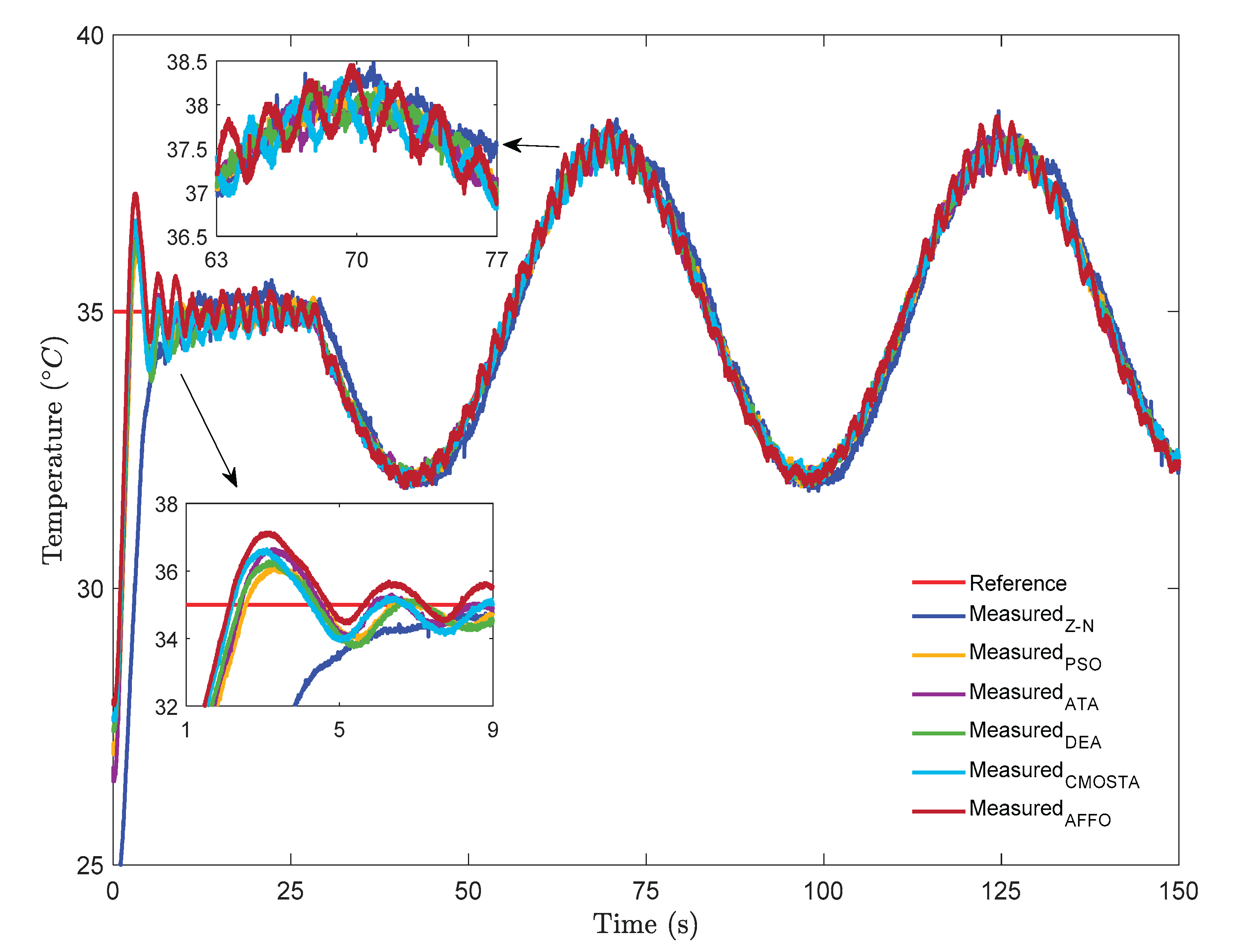
Figure 3.
Error signals of all optimization methods under step + sinusoidal reference signal.
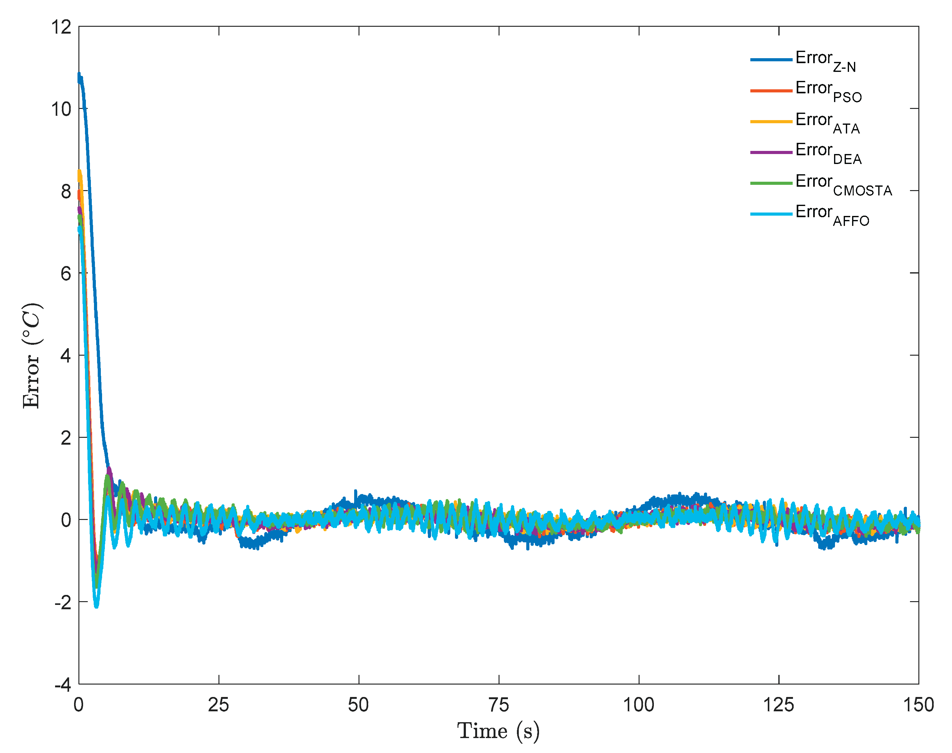
Figure 4.
Control signals of all optimization methods for step + sinusoidal reference signal.
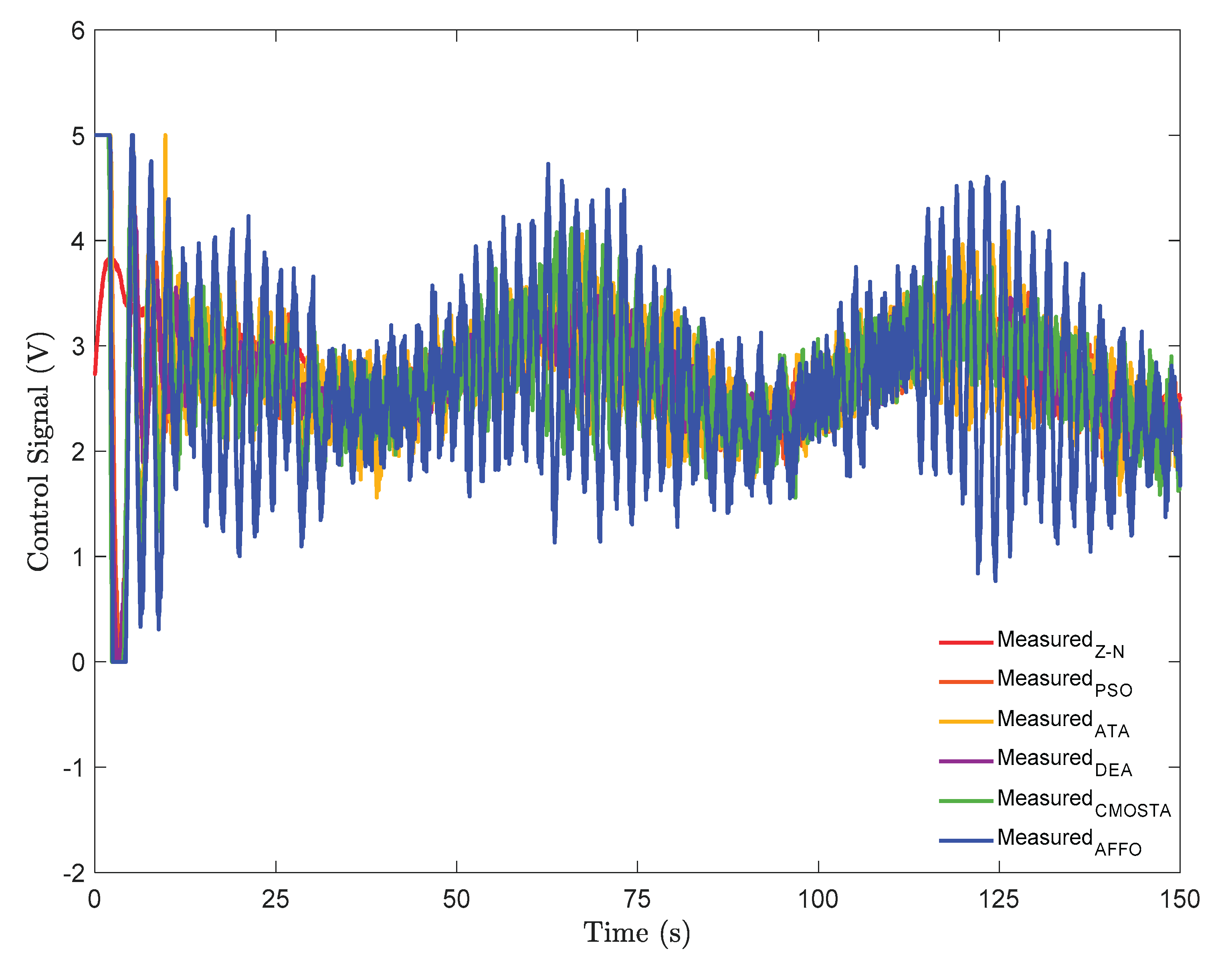
Figure 5.
Experimental results of all optimization methods under step + square reference signal.
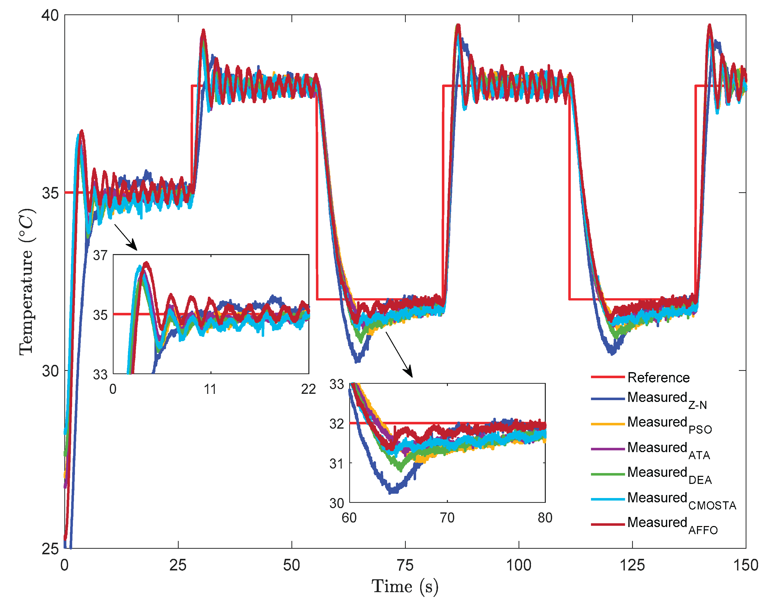
Figure 6.
Error signals of all optimization methods under step + square reference signal.
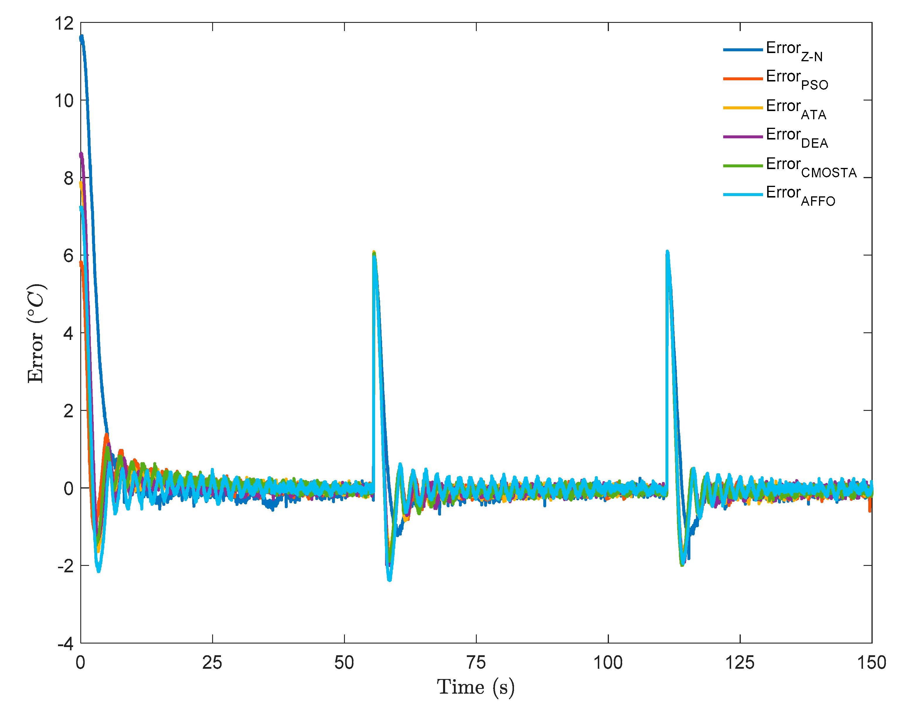
Figure 7.
Control signals of all optimization methods for step + square reference signal.
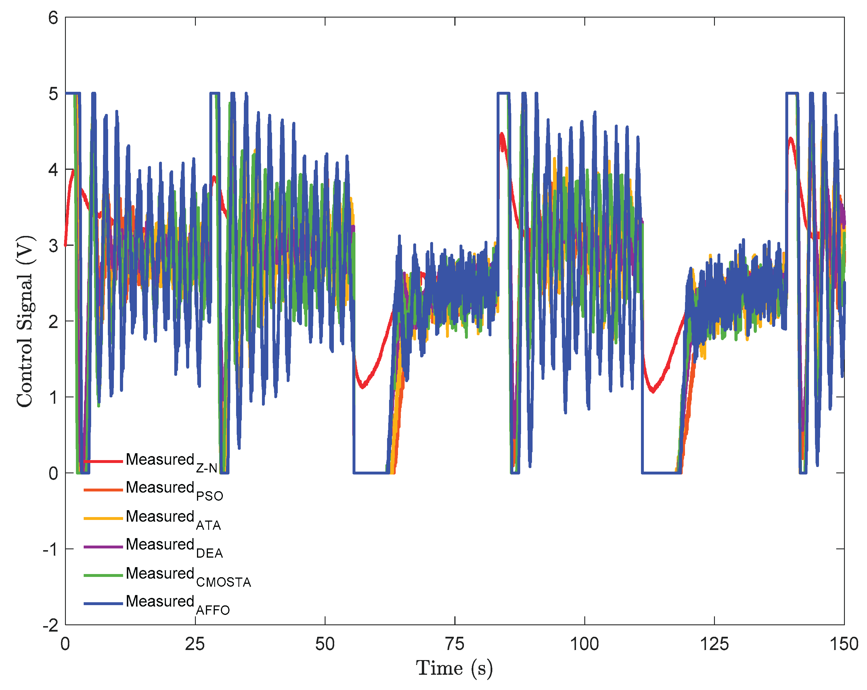
Figure 8.
Experimental results of all optimization methods under step + sawtooth reference signal.
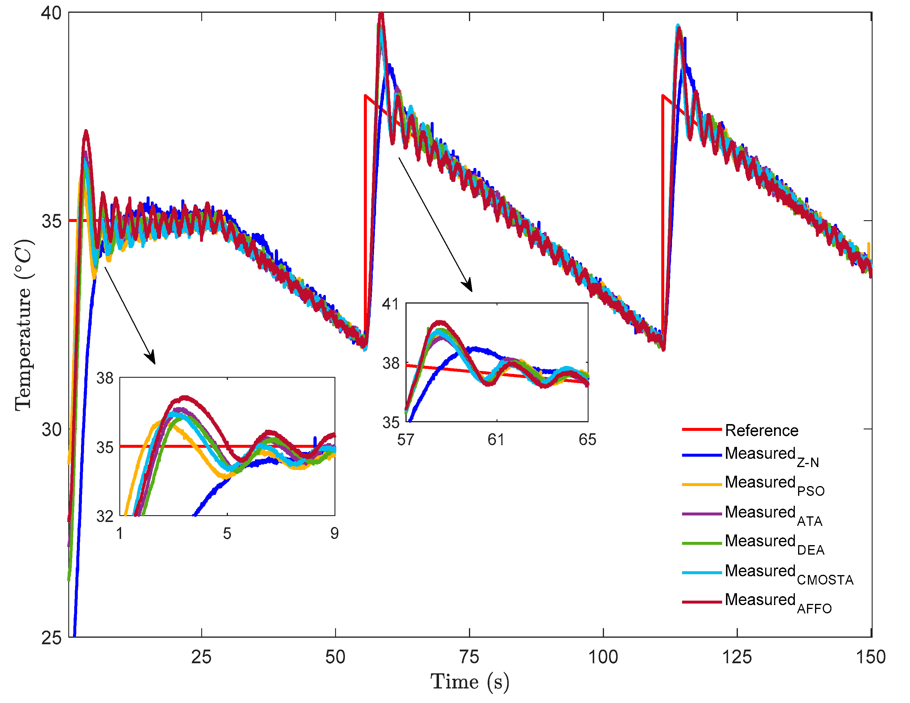
Figure 9.
Error signals of all optimization methods under step + sawtooth reference signal.
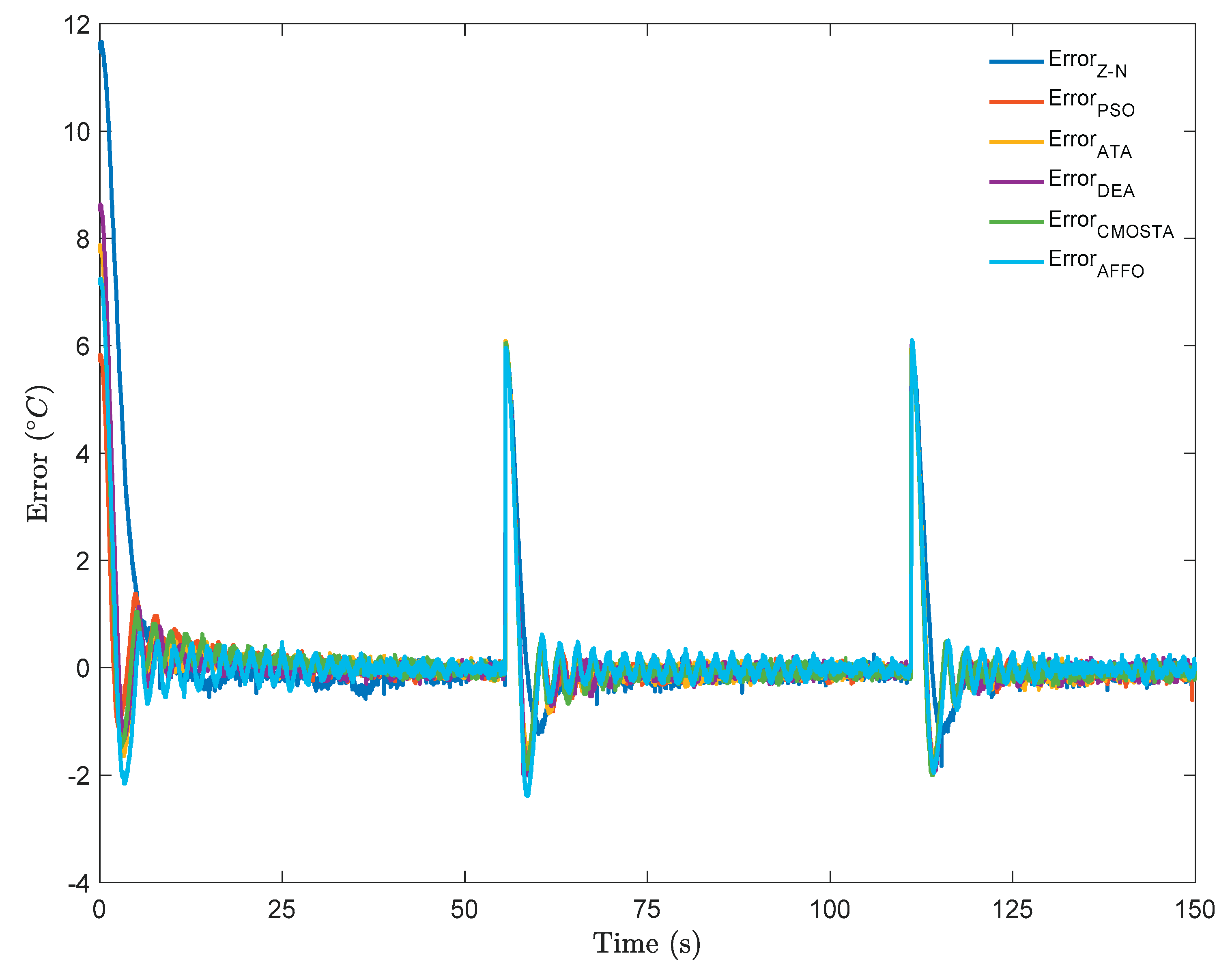
Figure 10.
Error signals of all optimization methods under step + sawtooth reference signal.
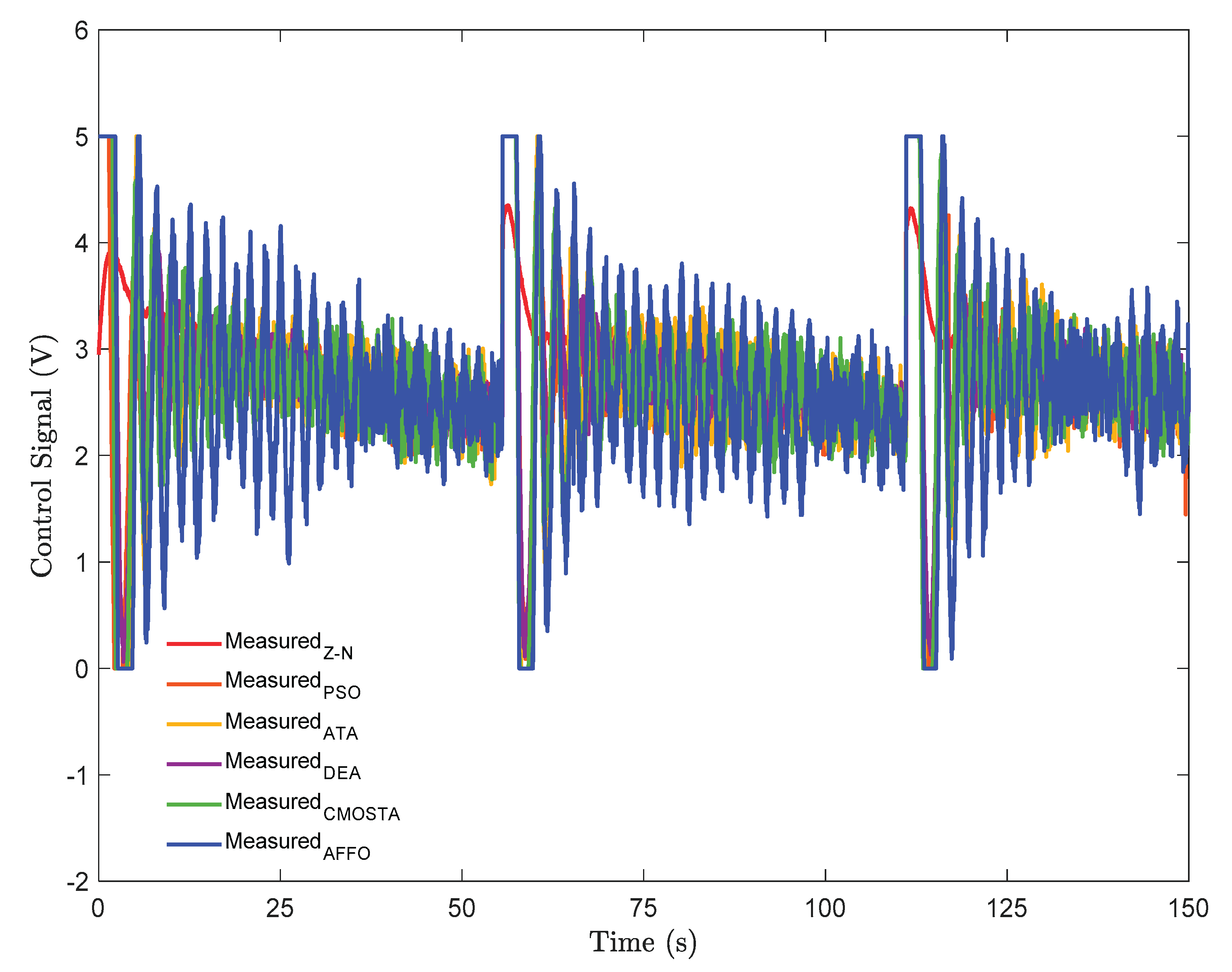
Table 1.
The MAE values of all optimization methods for step + sinusoidal reference signal [16].
Table 1.
The MAE values of all optimization methods for step + sinusoidal reference signal [16].
| Symbol | Description | Value | Unit |
| HFE dimensions | 50x15x10 | cm | |
| HFE mass | 0.5 | kg | |
| Blower nominal input voltage | 6 | V | |
| B | Blower nominal airflow | 36 | CFM |
| Blower nominal airflow (in SI units) |
1.02 | ||
| Max wind speed | 159.4 | m/min | |
| Blower max speed | 2700 | RPM | |
| Heater max power (at 5 V) | 400 | W | |
| Temperature sensor calibration gain |
20 | ||
| A | Cross sectional area | 0.0064 | |
| Current power requirements (maximum current) |
5 | A | |
| Heat flow voltage power requirements |
120-240 | VAC |
W = watt, VAC = volts alternating current, V = volt, s = second, cm = centimeter, m = meter, A = ampere, kg = kilogram.
Table 2.
The controller parameter values obtained via each optimization methods.
| Methods | Kp | Ki |
| Z-N | 0.2550 | 0.0941 |
| PSO | 2.0010 | 0.1902 |
| ATA | 3.1957 | 0.1882 |
| DEA | 1.8180 | 0.1986 |
| CMOSTA | 3.0180 | 0.1730 |
| AFFO | 1.9852 | 0.0347 |
Table 3.
The MAE values of all optimization methods for step + square reference signal.
| Methods | Step | Sinusoidal | Step + Sinusoidal |
| Z-N | 1.3655 | 0.7751 | 0.8772 |
| PSO | 0.6468 | 0.7483 | 0.7294 |
| ATA | 0.6443 | 0.7150 | 0.7018 |
| DEA | 0.6006 | 0.7014 | 0.7005 |
| CMOSTA | 0.6537 | 0.7107 | 0.7100 |
| AFFO | 0.7966 | 0. 7357 | 0.7192 |
Table 4.
The MAE values of all optimization methods for step + sawtooth reference signal.
| Methods | Step | Sinusoidal | Step + Sinusoidal |
| Z-N | 1.3413 | 0.3334 | 0.5215 |
| PSO | 0.6525 | 0.2665 | 0.3354 |
| ATA | 0.6593 | 0.2635 | 0.3374 |
| DEA | 0.6438 | 0.2603 | 0.3310 |
| CMOSTA | 0. 6604 | 0.2617 | 0.3342 |
| AFFO | 0.6716 | 0.2803 | 0.3533 |
Table 5.
The improvement table of all optimization methods for step + sinusoidal reference signal.
| Methods |
Step (wrt. Z-N) |
Sinusoidal (wrt. Z-N) |
Total Improvement (wrt. Z-N) |
| PSO | %52.37 | %62.52 | %57.30 |
| ATA | %50.63 | %62.21 | %50.42 |
| DEA | %54.06 | %69.24 | %58.04 |
| CMOSTA | %50.99 | %65.49 | %48.42 |
| AFFO | %53.29 | %55.39 | %43.83 |
Table 6.
The improvement table of all optimization methods for step + square reference signal.
| Methods |
Step (wrt. Z-N) |
Square (wrt. Z-N) |
Total Improvement (wrt. Z-N) |
| PSO | %52.63 | %3.45 | %16.84 |
| ATA | %52.81 | %7.75 | %19.99 |
| DEA | %56.01 | %9.50 | %20.14 |
| CMOSTA | %52.12 | %8.3 | %19.06 |
| AFFO | %41.66 | %5.08 | %18.01 |
Table 7.
The improvement table of all optimization methods for step + sawtooth reference signal.
| Methods |
Step (wrt. Z-N) |
Sawtooth (wrt. Z-N) |
Total Improvement (wrt. Z-N) |
| PSO | %51.35 | %20.06 | %35.68 |
| ATA | %50.84 | %20.96 | %35.30 |
| DEA | %52.00 | %21.92 | %36.52 |
| CMOSTA | %50.76 | %21.50 | %35.91 |
| AFFO | %49.92 | %15.92 | %32.25 |
Disclaimer/Publisher’s Note: The statements, opinions and data contained in all publications are solely those of the individual author(s) and contributor(s) and not of MDPI and/or the editor(s). MDPI and/or the editor(s) disclaim responsibility for any injury to people or property resulting from any ideas, methods, instructions or products referred to in the content. |
© 2025 by the authors. Licensee MDPI, Basel, Switzerland. This article is an open access article distributed under the terms and conditions of the Creative Commons Attribution (CC BY) license (http://creativecommons.org/licenses/by/4.0/).
Copyright: This open access article is published under a Creative Commons CC BY 4.0 license, which permit the free download, distribution, and reuse, provided that the author and preprint are cited in any reuse.


