
Submitted:
25 November 2025
Posted:
27 November 2025
You are already at the latest version
Abstract
This paper examines advancements in climate modeling, emphasizing integrated, physics-grounded and process-oriented approaches to enhance predictive reliability. It underscores the critical role of multiphase phenomena in atmospheric systems, including interfacial heat and mass transfers, and the integration of empirical data and high-resolution observational networks. Coupled with targeted laboratory and numerical experiments, these elements refine the physical basis of climate models. Efforts focus on addressing model limitations, including feedback uncertainties and challenges in AI/ML integration. A central focus is placed on “Statistical-Induced Uncertainties” (systemic biases introduced by spatio-temporal averaging, data interpolation, and ensemble processing) which propagate across modeling stages and may obscure physical interpretations. By embedding empirical rigor and prioritizing transparency, the study advocates for interdisciplinary collaboration to fill observational gaps, especially in under-observed regions, with statistical approaches aligned with physical interpretability. The paper highlights the value of ensemble modeling and AI, not as substitutes but as complements to physics-driven frameworks, supported by clear interpretive methods that anchor models in fundamental process closure. This integrated approach is essential for advancing climate projections and informing effective responses to global climate challenges.
Keywords:
climate modeling
; Statistical-Induced Uncertainties (SIUs)
; physical process closure
; multiphase energy transfers
; ensemble diagnostics
; AI/ML in climate science
; unified phenomenological calibration
1. Introduction
Since the pioneering General Circulation Models (GCMs) by Manabe (Manabe and Wetherald, 1967), climate science has advanced significantly. Innovations in observational technology and interdisciplinary modeling have transformed our understanding of Earth’s complex climate systems. Much of this progress has relied on a dual movement: the intensification of observational campaigns and the growth of interdisciplinary frameworks combining physics, statistics, and data science. Since the pioneering General Circulation Models (GCMs) by Manabe and Wetherald (1967), climate science has evolved through the convergence of observational advances and interdisciplinary modeling frameworks. A key driver of this progress lies in the refinement and integration of climate indicators—variables that capture long-term variability and anthropogenic trends. Enhanced by high-resolution sensors such as OCO-2 and GOSAT (Reynolds et al., 2002; Hansen et al., 2010; Liang et al., 2019), these indicators are synthesized by global networks (e.g., GAW, NOAA) to strengthen the empirical foundations of GCMs and Earth System Models (ESMs) (Dufresne et al., 2013).
On the other hand, high-resolution satellite missions like MODIS and AIRS have significantly improved the spatial and temporal resolution of climate indicators. Yet, coverage remains uneven, especially in polar and tropical regions with difficult access and limited observational infrastructure (Massom et al., 2018). Addressing these regional disparities is essential to reduce uncertainty in modeling precipitation and cloud variability (IPCC, 2021; Morice et al., 2012), and to enhance the phenomenological representativeness of process-level dynamics.
Managing uncertainty is not a peripheral concern but a structural feature of climate modeling. Reanalysis techniques—such as ERA5 and MERRA-2—play a critical role in harmonizing observational datasets (Balmaseda et al., 2013, Pelosi et al. 2020), improving regional coherence (Monier et al., 2016), and facilitating long-term continuity (Simmons et al., 2017; Hansen et al., 2023). Yet, these tools do not eliminate epistemic limitations, particularly in data-sparse regions where observational gaps amplify uncertainty (Hawkins and Sutton, 2009). Acknowledging these limits is a prerequisite for model transparency and interpretive robustness.
Understanding climate interactions requires a process-level grasp of feedback loops, such as those involving albedo, greenhouse gases, or cloud microphysics (Loeb et al., 2024; Bony et al., 2015). These non-linear dynamics, exemplified by the amplification of Arctic warming through sea-ice reduction (Meier et al., 2014), highlight the structural limits of scale-agnostic modeling. Echoing the argument developed in Chahed (2025), this paper aligns with the call for integrative modeling frameworks that do not obscure small-scale complexity behind aggregate variables (Reichstein et al., 2019).
Complementing physically based approaches, data-driven methods—particularly AI and ML—offer novel avenues for sub-grid parameterization and pattern discovery, especially for localized phenomena (Bolton and Zanna, 2019). These techniques have demonstrated potential in modeling processes like cloud formation and radiative forcing (Baño-Medina et al., 2020; Schneider et al., 2024). However, such methods must be cautiously framed within a physically coherent logic, since their smoothing effects and black-box nature may introduce epistemic opacity (Rolnick et al., 2022).
In line with recent calls for more reflective and responsible uses of climate models—such as Chahed (2025) and Koutsoyiannis (2025), which framed modeling as a practice shaped by epistemological, institutional, and normative considerations—the limitations in transparency and interpretability of many current modeling approaches raise critical concerns, especially in the context of decision-making and scientific validation. Recent philosophical analyses of climate modeling emphasize that assessing a model’s adequacy-for-purpose is essential when such models inform public policy (Winsberg and Harvard, 2024). Beyond technical accuracy, ethical dimensions further complicate the picture, highlighting the need for explicit strategies to manage value-laden judgments and ensure both accountability and democratic legitimacy in modeling practices (Winsberg, 2024). In this context, this article offers a thematically aligned contribution: it shifts the emphasis toward operational diagnostics and data integration strategies designed to enhance the credibility and applicability of climate simulations across scales and contexts.
This article offers a thematically aligned contribution. It shifts the emphasis toward operational diagnostics and data integration strategies designed to enhance the credibility and applicability of climate simulations across scales and contexts. Focusing on process-oriented approaches, structural diagnostics, and storyline-based methods, this work emphasizes modeling strategies that reinforce physical plausibility, interpretability, and robustness. Special attention is given to observationally grounded modeling, combining advanced monitoring networks with field-based calibration in under-observed regions (Newcomer et al., 2023). The article also In line with recent calls for more reflective and responsible uses of climate models—such as Chahed (2025) and Koutsoyiannis, D. (2025), which framed modeling as a practice shaped by epistemological, institutional, and normative considerations,
introduces and elaborates the concept of Statistical-Induced Uncertainty (SIU), highlighting how statistical operations—such as averaging, interpolation, or bias correction—can inadvertently propagate epistemic uncertainty and distort physical coherence. By foregrounding phenomenological accuracy and methodological transparency, this study contributes to an emerging agenda aimed at reconciling statistical processing with physical realism. It addresses persistent sources of structural bias and proposes concrete pathways to improve the trustworthiness of climate models in both scientific and policy arenas.
2. Progress and Challenges Across CMIP Climate Model Generations
2.1. CMIP Climate Models: Benchmarking and Intercomparison Frameworks
Introduced in the early 2000s under the CMIP, Earth System Models (ESMs) were designed to deepen our understanding of climate system interactions by integrating a variety of geophysical, thermodynamic, and dynamic processes. They provide a formal framework for evaluating the structural assumptions and parameterizations that shape climate projections. Synchronized with each major IPCC report cycle, these models support comparative assessments across generations. As emphasized in Chahed (2025), while model outputs are often aggregated into ensemble means, the underlying diversity in structure and process representation demands closer scrutiny. This calls for not just performance benchmarking, but also process-oriented diagnostics (Xie et al., 2022), which enhance transparency and traceability across modeling stages. Each CMIP phase (CMIP3–5–6) introduced notable improvements, yet structural divergences in radiative fluxes, aerosol-cloud interactions, and biosphere feedbacks persist. Differences in spatial resolution, data assimilation, and baseline assumptions continue to influence the robustness of projections (Frölicher et al. 2018; Tierney et al., 2020).
Furthermore, process-oriented evaluations highlighted by Xie et al. (2022) underscore the importance of using intercomparison in the CMIP6 framework to refine parameterizations. Each CMIP phase (CMIP3-5-6) introduced notable improvements in spatial resolution and in the representation of physical and chemical processes (Flato et al., 2014). ESMs simulate exchanges of heat, carbon, and other matter flows between domains (atmosphere, ocean, cryosphere, and biosphere), with an emphasis on key processes like cloud formation, precipitation, and land-atmosphere interactions—critical for capturing climate feedbacks. Advancements in CMIP6, particularly through process-oriented evaluations, have further addressed gaps in parameterization accuracy, as discussed by Meehl et al. (2020). Among these, albedo, water vapor, and cloud cover feedbacks remain pivotal to the global energy budget and projections of surface air temperature (SAT) (IPCC, 2021, Chapter 7; Calisto et al., 2014). Despite structural similarities, ESMs differ significantly in parameterization choices and baseline assumptions, which strongly influence their climate projections. For example, models vary in their representation of specific physical processes, such as solar and infrared radiative fluxes (shortwave radiation, SWR, and longwave radiation, LWR), which are essential for understanding warming mechanisms in the atmosphere and oceans (Frölicher et al. 2018). Differences in spatial and temporal resolution and in data assimilation techniques also contribute to varying projections (Tierney et al., 2020).
Inter-model comparisons in the CMIP framework rigorously test ESMs against historical observations, enhancing their reliability (IPCC, 2021, Chapter 3). However, significant uncertainties persist, particularly in processes such as sea ice formation and ocean heat exchanges. Emulators—simplified models designed to efficiently replicate ESM behavior—complement ESMs by refining projections of future climate conditions and facilitating strategic decision-making. By simulating ESM behavior for key variables like surface temperature and sea level across various scenarios, emulators enhance flexibility and reliability, making climate models more accessible to diverse applications and audiences (IPCC, 2021, Chapter 4).
2.2. Progress and Evolution of Climate Model Performance from CMIP3 to CMIP6
The progression from CMIP3 to CMIP6 shows clear improvement in simulating large-scale variables such as surface air temperature (SAT) and sea level pressure. However, as highlighted in Chahed (2025), persistent challenges in modeling variables like precipitation and cloud feedbacks reveal the limitations of current parameterizations and grid resolutions. Small-scale convective and radiative processes remain under-resolved, even as model accuracy improves for SAT. Figure 1 illustrates this tension between statistical correlation and physical representativity—an issue also explored in the earlier article through the lens of uncertainty epistemology. The dispersion in SAT across models, despite overall improvements, suggests that tuning rather than fundamental process understanding may drive accuracy gains. As Chahed (2025) notes, this raises critical questions on how models achieve predictive skill: through physical realism or statistical compensation. This paper further argues that process-oriented and emulation approaches are essential to clarify such ambiguities and improve interpretability across use cases.
Simulating precipitation accurately remains particularly challenging as it requires capturing detailed convective dynamics and cloud formation processes that exceed the capabilities of current model resolutions (Shin and Hong, 2015; Fathalli et al. 2019). Additionally, global climate models (GCMs) typically perform better in temperature simulations than in predictions of precipitation and hydrological dynamics (Besbes and Chahed, 2023). However, even their temperature projections exhibit limitations when evaluated against long-term observational records. The comparative study by Koutsoyianniset al. (2008), using over a century of temperature and precipitation data revealed that model outputs often diverge significantly from observed trends, even at the climatic 30-year scale.
Figure 1 illustrates the correlation between three generations of climate models (CMIP3-5-6) and observational data for near-surface air temperature (SAT), precipitation, and sea level pressure, with individual models represented by short lines and ensemble averages by longer lines.
Examining Figure 1 reveals key insights into the evolution of climate model accuracy across generations, particularly in capturing nonlinear interactions among climate parameters. While improvements in SAT accuracy are evident, with CMIP6 models nearing near-perfect correlations, similar advancements are lacking for precipitation and sea level pressure, which exhibit lower correlations. This discrepancy highlights the difficulty of capturing complex interactions and feedbacks inherent in the climate system. Furthermore, the increased dispersion in model results, especially for SAT, reflects persistent variability in model predictions despite overall advancements.
Furthermore, the increased dispersion in model results, particularly for SAT, reveals a paradoxical dynamic: while ensemble averages improve, individual model outcomes become more scattered. This dispersion suggests that improvements in SAT accuracy may stem more from ad hoc model tuning than from convergent advances in theoretical understanding. If physical mechanisms were consistently resolved, we would expect systematic progress across all key indicators, not just SAT. This persistent discrepancies across CMIP generations underscore the need for more process-sensitive evaluations of model performance. Climate models remain limited in capturing regional heterogeneity, particularly for precipitation dynamics and cloud radiative feedbacks, where subgrid-scale processes are often inadequately represented. These limitations constrain the reliability of regional climate projections and hinder robust risk assessments. Despite improved spatial resolution, models continue to face challenges with convective cloud formation, aerosol-cloud-radiation coupling, and boundary-layer dynamics. These unresolved processes contribute to structural uncertainties that escape standard validation frameworks, reinforcing the need for diagnostics grounded in physical processes rather than bulk statistical agreement. As highlighted in multiple intercomparison efforts, including CMIP6 evaluations (IPCC, 2021), such biases persist even in ensemble means, limiting the robustness of policy-relevant insights.
In response to these limitations, process-oriented evaluation has gained traction as a promising strategy. It shifts model assessment from statistical averages to comparisons with physically interpretable, mechanism-based metrics. By isolating key dynamics—such as convective initiation, moisture transport, or albedo feedbacks—these diagnostics expose underlying structural biases that ensemble statistics often conceal. This fine-grained analysis complements the broader epistemological critique developed in Chahed (2025), by offering operational tools to enhance model fidelity. In parallel, physically constrained storylines emerge as powerful narrative frameworks that align climate scenarios with plausible dynamic trajectories. These storylines provide actionable insights for regional planning and adaptation, while preserving physical realism without relying on probabilistic assumptions
3. Feedbacks, Interfaces, and Nonlinear Interactions in the Climate System
3.1. Observational Indicators and Multi-Domain Climate Monitoring
A review of key reports and studies from authoritative organizations such as the IPCC and WMO identifies a set of core Essential Climate Variables (ECVs) crucial for climate monitoring. These include Surface Air Temperature (SAT), Sea Surface Temperature (SST), Sea Ice Extent (SIE), Cloud Cover (CC), Shortwave Radiation (SWR), Longwave Radiation (LWR), Wind Patterns (WP), Humidity Levels (HL), Soil Moisture (SM), Ocean Heat Content (OHC), Carbon Dioxide (CO₂), Methane (CH₄), and Precipitation (P).
These indicators are essential not only for observational diagnostics but also for process-level validation and model benchmarking in ESM development. They span all major domains—atmosphere, ocean, cryosphere, and land surface—and are instrumental in representing feedback mechanisms such as the greenhouse effect, the hydrological cycle, and the albedo effect. In the terrestrial domain, enhanced Earth observation (EO) optical data now provide high-precision estimates of surface parameters. When coupled with canopy reflectance models, these observations improve land surface representation and reduce reliance on empirical approximations, (D’Urso et al., 2008). Estimation of land surface parameters through modeling inversion of earth observation optical data. In Advances in Modeling Agricultural Systems (pp. 317-338). Boston, MA: Springer US.
Figure 2 illustrates the core climate indicators and their interconnections, highlighting feedback loops that drive climate processes. These variables serve as critical metrics for capturing the intricate processes driving climate change, (IPCC, 2021; Hansen et al., 2010). This figure shows how these indicators form interlocking feedback loops across subsystems, underscoring the inherently coupled and nonlinear nature of the climate system.
This framing aligns with CMIP’s diagnostic architecture, where accurate representation and evaluation of these ECVs remain pivotal for constraining uncertainties and enhancing interpretability. The selection of these indicators reflects not only physical relevance, but also continuity of long-term records and integration into model-data assimilation frameworks.
Data is sourced from networks that combine terrestrial, aerial, and satellite observations. High-resolution satellite missions and ground-based stations are essential to calibrate and constrain model simulations of key climate indicators. Networks like the Global Atmosphere Watch (GAW) and NOAA’s program provide continuous monitoring of CO₂ and CH₄ levels, which is crucial for tracking atmospheric carbon dynamics and informing carbon cycle models such as Carbon Tracker (IPCC 2021, Chapter 6). Additionally, Pattanaik (2022) emphasizes the value of combining in situ measurements with model outputs, especially in regions sensitive to monsoon variability. Satellite missions such as OCO-2, GOSAT, and CERES provide dense global coverage of carbon fluxes and radiative parameters, facilitating detailed assessments of spatial and seasonal variability (Friedlingstein et al., 2006). Surface temperature datasets (SAT, SST) from HadCRUT, NOAA, and GISTEMP ensure temporal continuity and robustness for model evaluation.
Complementing atmospheric observations, satellite missions and ship-based surveys—such as HadISST and ERSST—monitor sea surface temperature (SST) and energy fluxes across the ocean–atmosphere interface. These benchmark datasets enable robust detection of ocean warming trends. They are further enhanced by reanalysis products like ERA5 and MERRA-2, which assimilate satellite, buoy, and ship-based observations to generate coherent, long-term climate records (Reynolds et al., 2002). Such integrated products are crucial for capturing historical SST variability and calibrating ocean components of Earth System Models.
Cloud Cover (CC) plays a critical role in modulating the Earth’s radiative balance and is quantified via satellite missions such as CALIPSO (Cloud-Aerosol Lidar and Infrared Pathfinder Satellite Observations) and ISCCP (International Satellite Cloud Climatology Project) (Winker, 2023). These missions provide global datasets that feed directly into climate models, enhancing the simulation of radiative forcing and cloud feedbacks.
Aerosols, particularly organic and sulfated particles, also exert major influence on climate dynamics. They act as cloud condensation nuclei, thereby affecting cloud albedo and lifetime (Snoun et al., 2019). These particles originate from complex multiphase chemical and physical processes, often involving both natural and anthropogenic emissions (Bellakhal et al., 2020; Kumar et al., 2024). Their inclusion in Earth System Models improves the representation of indirect radiative effects and feedbacks. These observations are essential for simulating both the energy balance and hydrological cycles within climate models. Their utility is significantly enhanced by reanalysis products such as MERRA-2, which extend spatial and temporal coverage, particularly for cloud-related variables (Winker, 2023).
Shortwave Radiation (SWR) and Longwave Radiation (LWR)—measured by satellite missions like CERES—provide key estimates of solar energy reflection and infrared absorption, critical for understanding atmospheric heating processes. Reanalysis models help correct for regional observational biases, particularly in areas with persistent cloud cover or high elevation, where satellite signals can be obstructed (Stephens et al., 2020).
Precipitation data, essential for water cycle modeling, are compiled from global observational networks such as the GPCC and satellite missions like TRMM. These systems offer near-global rainfall estimates, although their accuracy can be reduced in arid and mountainous regions, where satellite retrievals are often challenged by surface interference and low signal-to-noise ratios (Adler et al., 2003).
Humidity levels, critical for cloud formation and extreme weather modeling, are captured via in situ stations and satellite sensors like AIRS and MODIS. These measurements are synthesized into reanalysis products to generate consistent vertical and temporal profiles of atmospheric moisture, enabling better detection of extreme climate phenomena (IPCC 2021, Chapter 8).
Soil moisture, a key variable for assessing drought risk and heatwave severity, is monitored through missions such as SMOS and ASCAT. These datasets are harmonized using reanalysis systems like GLDAS, which improve the spatial resolution and temporal coherence of moisture trends (Wagner et al., 2007; Albergel et al., 2013).
Sea Ice Extent (SIE), a critical polar climate indicator, is tracked by the National Snow and Ice Data Center and satellite platforms. These observations, often limited by harsh polar conditions, are refined using reanalysis products like ERA5, which fill spatial gaps and ensure continuity in long-term ice cover records (Cavalieri et al., 1984; Massom et al., 2018).
Wind pattern datasets, obtained from global meteorological stations and remote sensing missions such as QuikSCAT and ASCAT, play a pivotal role in characterizing heat and moisture transport across regions. These winds influence large-scale atmospheric circulation, drive ocean-atmosphere interactions, and contribute to the redistribution of energy within the climate system (Hersbach et al., 2020).
By integrating these wind observations with other satellite and in situ data, Earth System Models (ESMs) are supported by a multi-dimensional and highly resolved observational framework. This foundation is strengthened through reanalysis tools (e.g., ERA5, MERRA-2), which allow for greater temporal continuity and spatial coherence. Collectively, this integration enhances the credibility of climate scenarios and deepens understanding of nonlinear feedbacks and cross-domain dynamics in the Earth’s climate system (Dee et al., 2011; Compo et al., 2011).
3.2. Managing Uncertainty and Coherence in Multi-Source Climate Data
Observational data derived from terrestrial, oceanic, and satellite platforms provide the empirical basis for Earth System Models (ESMs) to evaluate climate responses to both natural and anthropogenic forcings. However, these datasets are inherently subject to multiple sources of error, including spatial and temporal resolution constraints, instrument calibration issues, and inconsistencies across methodologies. Mitigating these uncertainties is essential, as initial errors can propagate nonlinearly through simulation chains, thereby skewing model outputs and projections (Caldwell et al., 2016). To address this, Venkatasubramanian et al. (2001) propose diagnostic tools to identify and manage uncertainties, while Popp and Mittaz (2022) emphasize the importance of understanding uncertainty propagation mechanisms across model layers and timescales.
Systematic biases in climate time series—particularly for Surface Air Temperature (SAT), Sea Surface Temperature (SST), Sea Ice Extent (SIE), and greenhouse gas concentrations—often stem from sensor discrepancies, calibration drift, and natural interannual variability. For instance, SST and SIE satellite-derived estimates can be underrepresented in polar and high-altitude regions, leading to mischaracterization of warming patterns and ice loss anomalies (Simmons et al., 2017). Similarly, cloud cover datasets from ISCCP, CALIPSO, and MODIS carry greater uncertainty in equatorial and polar zones due to rapid atmospheric changes and limitations in optical and infrared resolution (Winker, 2023; Zhang et al., 2024). Soil moisture and precipitation data are particularly vulnerable to regional-scale inconsistencies, with precipitation datasets such as GPCC and TRMM often diverging because of heterogeneous sampling methods—especially over mountainous and arid regions where satellite-ground correspondence is weakest (Huffman et al., 2009).
Reanalysis methodologies, which blend observational datasets with numerical model outputs, are essential for constructing internally consistent global climate records. Projects such as ERA-Interim have significantly improved the coherence of long-term climate series by merging heterogeneous data streams—including satellite, ground-based, and radiosonde observations—into unified, gridded datasets (Dee et al., 2011). These methods generate high-resolution spatiotemporal fields for key variables like surface air temperature and precipitation, enabling precise trend analysis and regional anomaly detection. Reanalysis products are extensively employed to track global warming trajectories and serve as foundational tools for IPCC assessments aimed at disentangling anthropogenic signals from natural variability.
3.3. Coupled Feedbacks and Dynamic Interactions in the Climate System
Climate system dynamics emerge from multi-scale interactions that can either amplify (positive feedbacks) or dampen (negative feedbacks) environmental perturbations. For instance, Sea Surface Temperature (SST) strongly influences tropical atmospheric convection, while decreases in polar cloud cover enhance solar energy absorption, intensifying regional warming (Reynolds et al., 2002; Wild, 2020). These coupled mechanisms govern seasonal patterns in temperature and humidity, establishing tight feedbacks between SAT and precipitation (Trenberth and Fasullo, 2012; Bony et al., 2015).
Central to this regulation are Shortwave Radiation (SWR) and Longwave Radiation (LWR), which form the backbone of Earth’s energy exchange. SWR raises diurnal temperatures, while LWR retains nocturnal heat, smoothing diurnal fluctuations (Loeb et al., 2024). These radiative fluxes interact nonlinearly with greenhouse gases like CO₂ and CH₄, which absorb LWR and intensify the greenhouse effect, thus reinforcing surface air temperature (SAT) increases (Andrews et al., 2012).
Atmospheric and soil moisture play a crucial regulatory role in climate dynamics, particularly in modulating temperature and precipitation regimes. Elevated atmospheric humidity functions as a thermal buffer, reducing temperature extremes by trapping outgoing longwave radiation (Soden and Held, 2006). Meanwhile, soil moisture mediates SAT via evapotranspiration processes: moist soils dissipate energy through latent heat, whereas dry soils enhance surface warming (Seneviratne et al., 2010).
The Ocean Heat Content (OHC) acts as a vast thermal reservoir, mitigating abrupt atmospheric changes by absorbing surplus heat. Yet, as oceans warm, their capacity to buffer declines, intensifying both SST and SAT trends (Harzallah and Sadourny, 1995; Cheng et al., 2019). Lastly, wind circulation patterns, such as trade winds, redistribute heat and humidity across regions: they transport warm air toward equatorial zones, thereby regulating SAT and modifying SST through upwelling mechanisms (Hersbach et al., 2020).
3.4. Energy Budgets and Multiphase Transfers Across Climate System Interfaces
The global energy budget constitutes a core diagnostic in Earth System Models (ESMs), as it links key climatic variables such as Surface Air Temperature (SAT), Sea Surface Temperature (SST), and cloud cover. Radiative balances, governed by incoming shortwave solar radiation and outgoing longwave infrared radiation, drive the Earth’s warming trajectory, although substantial uncertainties persist despite improved satellite calibration techniques (Reynolds et al., 2002; Wild, 2020).
Greenhouse gases (GHGs), particularly CO₂ and CH₄, reinforce the greenhouse effect, while Arctic sea ice decline contributes to warming through albedo reduction—a positive feedback that amplifies regional and global energy absorption (Andrews et al., 2012; Trenberth et al., 2003). Additionally, phase change processes, such as evaporation and condensation, are essential for cloud dynamics and thermodynamic regulation, influencing precipitation patterns and model predictability (Trenberth et al., 2009; Bony et al., 2015).
Interactions between climate subsystems generate dynamic feedback loops, whereby perturbations in one domain propagate across others, producing amplifying (positive) or moderating (negative) effects. Feedbacks involving cloud microphysics, aerosols, and surface albedo are particularly sensitive to multiphase interactions occurring across atmospheric layers and interfaces. As highlighted by Stenchikov et al. (2022), current global climate models often fail to capture the early evolution of complex multicomponent systems—such as volcanic clouds composed of ice, SO₂, SO₄, ash, and water vapor—due to limitations in spatial resolution and insufficient physical parameterizations. Furthermore, the underlying dynamic and chemical mechanisms behind the high sensitivity of stratospheric aerosol optical depth (SAOD) to injection height remain largely untested in fully interactive models. Key processes, such as the effects of water vapor injected during eruptions and the chemical aging of volcanic ash are seldom represented in models with comprehensive chemistry and detailed microphysics (. When enhanced to incorporate finer-scale processes and eruption-specific dynamics, regional models can provide critical insights into the dispersion patterns and radiative impacts of such systems, underscoring the value of process-resolving approaches for robust climate feedback analysis. In this context, local analysis of turbulent multiphase flows offers valuable insight into interfacial energy and mass exchanges, influencing convection, condensation, and radiative transfer (Chahed et al., 2003; Ayed et al., 2007).
Recent studies on Arctic cyclone dynamics reveal that multiphase cloud systems accelerate sea ice melt and redistribute latent heat, reshaping local and regional energy budgets (Liang et al., 2019). Moreover, the hydrological cycle, through atmospheric moisture and cloud feedbacks, regulates tropical convection and precipitation intensity. Ice-albedo mechanisms, particularly in polar latitudes, further reinforce regional warming by reducing reflective surfaces (Loeb et al., 2022). Thermodynamic exchanges between SAT and SST, mediated by winds and surface fluxes, structure seasonal cycles and regional variability (Cheng et al., 2019).
The Earth’s energy budget is deeply shaped by phase transition processes, which regulate latent heat exchanges at the interfaces of the atmosphere, ocean, and cryosphere. Evaporation, condensation, and crystallization alter energy fluxes by either releasing or absorbing latent heat, with direct consequences on regional and global thermodynamic balances (Loeb et al., 2024). Capturing these multiscale nonlinear dynamics remains a major challenge for modeling, requiring granular, phenomenologically accurate parameterizations (Jabnoun and Harzallah, 2024; Stubenrauch et al., 2024).
Yet, current representations are constrained by the limited understanding of coupled ice-ocean-atmosphere interactions, especially under extreme or transitional conditions (Reynolds et al., 2002). These limitations are exacerbated by the inherently nonlinear nature of climate feedbacks, which defy simple linear approximations and call for robust, process-aware modeling strategies (Stephens et al., 2022). Such frameworks are necessary to account for the cascading effects and interconnected feedbacks that characterize the functioning of the Earth system.
4. Scientific and Methodological Barriers in Climate Modeling: Nonlinear Feedbacks and Statistical-Induced Uncertainties
4.1. Nonlinear Mechanisms and Mathematical Constraints: A Differential Perspective
Climate models encounter significant limitations when attempting to represent the complexity and nonlinearity of feedback mechanisms operating across the climate system. These complexities arise from multiscale interactions, including aerosol nucleation, phase transitions, and cloud-radiation processes, which can either amplify or dampen atmospheric responses (Loeb et al., 2022). The nonlinear coupling of physical processes across different temporal and spatial scales complicates predictability and increases model sensitivity (Lorenz, 1963; Pierrehumbert, 2010; Lenton et al., 2008).
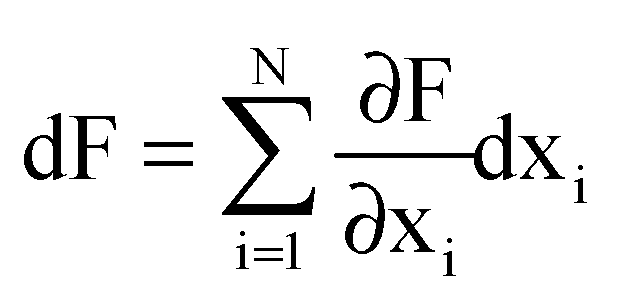
To conceptualize these challenges, one may turn to elementary mathematical formalisms, such as the total differential, which help illustrate the limits of inference and representation in climate science. Consider a parameter F that depends on multiple interdependent parameters Xi, (e.g., temperature, humidity, greenhouse gas concentrations, etc.). Here, the total differential of F expresses its infinitesimal variation based on infinitesimal variations in each parameter Xi:
In this formulation, the partial derivatives indicate the sensitivity of F to changes in each contributing parameter Xi. These derivatives theoretically enable a decomposition of influence across variables. However, in a real-world climate system, such derivatives are often ill-defined or poorly constrained due to the nonlinearity, feedback loops, and dependencies among variables. To analyze the specific influence of a given parameter Xj on F, the total differential can be rearranged to isolate its contribution:
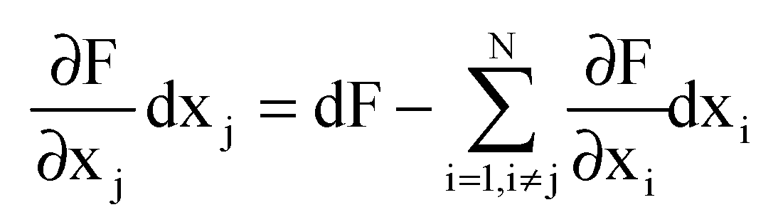
This expression reveals a major methodological challenge: to determine the effect of Xj on F, one must precisely know the partial derivatives and variations of all other variables, which is rarely achievable with observational data alone.
Applying this framework to climate data analysis demonstrates that the uncertainty in partial derivatives and the entanglement of variables make causal attribution difficult. While observational data are vital for model calibration and validation, they often lack the spatial, temporal, and process-level resolution needed to decouple individual drivers. Furthermore, outputs are strongly shaped by initial conditions and embedded in feedback structures that are not yet fully understood.
Addressing these gaps requires the implementation of process-oriented benchmarking, involving case-specific model evaluations under well-defined physical scenarios. This would help reveal alignment or divergence between model outputs and observed processes, thereby illuminating weaknesses in parameterization or model structure. To overcome these challenges, a systematic benchmarking of physical and microphysical processes through carefully designed case studies could illuminate where current models align or diverge from observed phenomena.
4.2. Spatio-Temporal Variabilities and Statistical-Induced Uncertainties in Climate Data Processing
Spatio-temporal averaging is essential for identifying long-term trends in climate systems, as it transforms localized and seasonal signals into global indicators that reflect decadal-scale changes (Brohan et al., 2006; Morice et al., 2012). Yet, these averages carry inherent uncertainties, stemming from non-uniform spatial coverage, temporal gaps, and variable data resolution across regions. To formalize spatiotemporal averaging this process, an instantaneous local climate variable F (e.g., temperature or precipitation) is mathematically decomposed into a mean field and a component f’ representing deviations from the average:
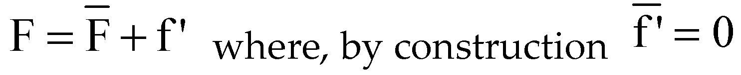
This decomposition helps assess how local short-term variability contributes to or diverges from long-term mean climate behavior. Here, () denotes a spatiotemporal averaging that verifies Reynolds’s rules, which notably include linearity and commutativity with derivatives—a key property in turbulence and climate diagnostics. The standard deviation of F is given by:
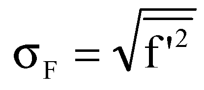
where effectively represents the variance of F, which quantifies its dispersion around the mean. The variance is critical for understanding internal variability, especially when interpreting differences between modeled and observed climate indicators.
To extend this reasoning to multivariate systems, we can express the total differential dF of a variable F (dependent on interrelated parameters xᵢ) in terms of its spatio-temporal mean and fluctuation components. Substituting the decomposition for each variable into the differential, this gives:
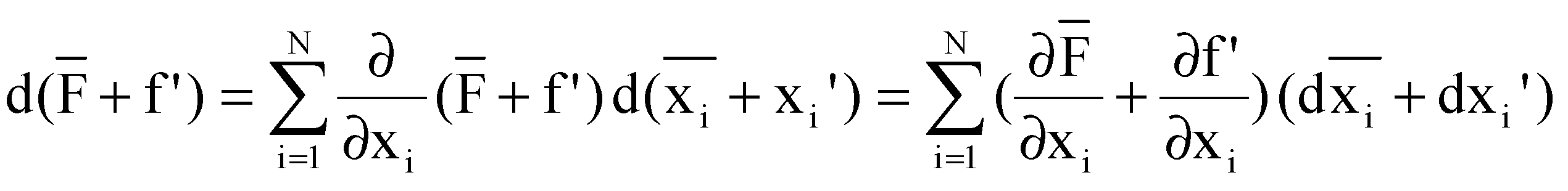
Developing and applying the averaging operator while noting that terms with f’ and xi’ averages are zero, this yields:
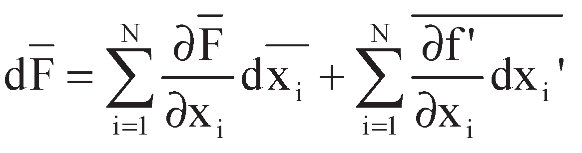
This formulation reveals that averaging nonlinear expressions introduces, besides the differential associated with the mean field of the variables (first term on the right side of the equation), covariances between fluctuations (las term on the right side of the equation), which do not vanish in general and thus alter the relationship between mean variables and their differentials.
Figure 3 visualizes how Statistical-Induced Uncertainties propagate through the pre- and post-processing stages of climate data modeling, particularly in regions with steep spatial gradients or limited observational coverage. This highlights a crucial methodological point: interpreting climate trends based solely on mean values—without accounting for the underlying fluctuations and variances—can introduce systematic misrepresentations. These are referred to as SIUs, and they accumulate across each processing stage, from raw data assimilation to model output interpretation.
5. Refining Climate Modeling Within a Unified Physically-Grounded Research Framework
5.1. Strengths and Limits of Climate Modeling Approaches
Current climate models—notably those developed within the CMIP framework (Eyring et al., 2016)—remain foundational for understanding global climate dynamics. However, the spatio-temporal averaging techniques they rely on, while necessary for long-term assessments, may introduce “Statistical-Induced Uncertainties”, particularly when extrapolated to regions with sparse observational coverage. Interpolation and reanalysis techniques can mitigate some of these limitations, but they rest on simplifying assumptions that introduce additional sources of uncertainty, reinforcing the need for methodological refinement (Cheng et al., 2019).
Ensemble modeling—which combines outputs from multiple climate models—aims to reduce individual-model biases, thereby yielding more robust and smoothed climate projections. The CMIP6 ensemble exemplifies this approach, offering a diverse range of global climate scenarios. Yet, interpreting ensemble outputs poses challenges, particularly due to intermodel dependencies and embedded structural biases. Tebaldi et al. (2021) stress the need for a nuanced interpretation of these ensembles. A fundamental epistemological question arises: should these ensembles be viewed as physical representations of climate systems, or rather as statistical constructs optimized for bias minimization? In practice, ensemble models embody a dual character—they improve global-scale projections, but their reliability at regional or fine scales requires cautious interpretation.
Data-driven approaches, including Artificial Intelligence (AI) and Machine Learning (ML), offer an empirical alternative by leveraging observed data to infer climate patterns. These models excel at detecting correlations and nonlinear relationships, without explicitly modeling physical mechanisms. However, as Loeb et al. (2024) demonstrate, such models may struggle to capture key processes like the radiative impacts of phase transitions. Statistical processing within ML frameworks often propagates uncertainties, especially when extrapolating beyond the scope of training data. Techniques such as regression analysis, empirical orthogonal functions, or Bayesian inference enable useful approximations of climate variable relationships—but they remain limited in capturing fine-scale, multiphase processes central to energy transfer.
Moreover, reliance on historical datasets risks embedding systemic biases, particularly in poorly instrumented regions. Advanced AI techniques, including neural networks and deep learning, can detect hidden patterns in high-dimensional data, yet lack transparency and physical interpretability. Rolnick et al. (2022) emphasize that AI models must be carefully aligned with physical principles to avoid misleading conclusions. Therefore, all data-driven models require rigorous validation and cautious use, particularly in predictive scenarios involving novel or extreme climate conditions.
5.2. Statistical Approaches in Climate Modeling: Reconciling Bias Corrections with Physical Coherence
Ensemble Climate Models: Balancing Bias Reduction and Phenomenological Integrity
Ensemble models combine outputs from multiple simulations to reduce systemic biases and produce more robust probabilistic projections. However, this aggregation may obscure inter-model covariance structures, which are critical for capturing fine-scale interactions and dynamic feedbacks. This underscores a key methodological tension: the trade-off between bias minimization and phenomenological fidelity. In this context, ensemble models are best understood as statistical constructs, optimized for robustness, rather than as faithful physical representations of the climate system.
AI and ML Algorithms: Enhancing Precision While Maintaining Transparency
Artificial Intelligence (AI) and Machine Learning (ML) offer powerful avenues for enhancing the granularity and accuracy of climate predictions, particularly when analyzing large, multidimensional datasets. However, their limited transparency and interpretability raise critical concerns, especially in the context of decision-making and scientific validation. Given the complexity and interdependence of climate processes, AI/ML methods should be used as complementary tools, not substitutes for physically based models. Their application is especially promising in controlled experimental contexts, where specific variables can be systematically isolated and manipulated to refine our understanding of key processes. supporting more physically consistent parameterizations in physics-driven models.
5.3. Enhancing Parameterizations in Physics-Based Models through Controlled Environments and Numerical Simulations
Establishing Global Controlled Testing Environments
Improving the predictive accuracy of physics-based climate models calls for the development of a global network of controlled testing environments, where key climate variables can be examined under well-defined, reproducible conditions. These environments—ranging from structured laboratory facilities to specialized field stations—are vital for investigating critical processes such as cloud microphysics, aerosol dynamics, and boundary-layer interactions. Targeted observational strategies, especially in data-sparse or climatically sensitive regions, are crucial for calibrating and validating feedback mechanisms. By filling key observational gaps, these setups contribute to more robust and transferable parameterizations, reinforcing the physical credibility of climate models. Ultimately, such efforts anchor predictive tools in empirical science, ensuring that fundamental physical insights inform model development and refinement.
Leveraging Numerical Simulations for Parameterization
Numerical simulations grounded in first-principles physics—notably Computational Fluid Dynamics (CFD), Large Eddy Simulations (LES), and Direct Numerical Simulations (DNS)—offer indispensable tools for exploring climate processes beyond empirical reach. In particular, multiphase CFD enables detailed representation of mass, momentum, and energy transfers in turbulent, multiphase environments, providing granular insights into interfacial dynamics (Mrabtini et al., 2017). These simulations allow the investigation of key microphysical processes—condensation, evaporation, nucleation—under conditions inaccessible to direct measurement. Their integration into larger-scale Earth system models strengthens parameterization schemes, especially for nonlinear and scale-coupled feedbacks. Embracing numerical experimentation thus plays a pivotal role in bridging theory, observation, and modeling, enhancing both predictive power and physical realism.
Advancing Research in Under-Observed Regions
Under-observed regions—notably the Arctic, tropics, and parts of the Southern Hemisphere—represent both a major challenge and opportunity for improving climate projections. These zones are often climatically sensitive yet severely lacking in observational coverage. Advancing research in these areas requires dedicated field campaigns, the deployment of cost-effective, adaptive sensor technologies, and the establishment of permanent or semi-permanent observation sites. Such efforts enable direct study of aerosol-cloud interactions, regional energy budgets, and boundary-layer dynamics under extreme or variable conditions. Coupled with high-resolution numerical simulations, this research mitigates spatial biases, strengthens global model calibration, and improves predictive fidelity across latitudinal and seasonal gradients.
5.4. Toward a Process-Oriented Benchmarking Framework for Climate Models
Integrating Observations, Simulations, and Collaboration
Advancing climate modeling demands a unified research architecture that combines empirical observations, high-fidelity simulations, and interdisciplinary collaboration. Central to this effort is the integration of multiphase dynamics, particularly across key system interfaces—cloud–aerosol, ocean–atmosphere, and ice–ocean boundaries—where nonlinear energy and mass exchanges dominate. A coordinated international strategy to refine and benchmark multiphase parameterizations, validated through controlled experimental setups, is crucial to closing the most persistent gaps in climate prediction. This iterative approach fosters productive feedback loops, where enhanced models drive targeted data collection, and new observations refine model assumptions. By prioritizing open access to shared observational platforms and harmonized datasets, this framework strengthens both model adaptability and physical integrity, effectively bridging fundamental science with decision-relevant projections.
Rethinking Model Intercomparison Programs
Model intercomparison programs like CMIP have significantly contributed to the standardization of outputs and the harmonization of evaluation protocols across climate modeling centers. However, their current structure tends to prioritize output alignment over physical realism, often emphasizing bias correction rather than process fidelity. As highlighted by Sherwood (2002), the field must move toward robust, physics-based benchmarks that rigorously test model closures, parameterizations, and the internal consistency of feedback mechanisms. This implies a shift from predominantly output-focused comparisons to process-oriented assessments, capable of revealing where models capture—or fail to capture—key physical dynamics. Such a reframing is essential for identifying structural weaknesses and for guiding the next generation of climate model development.
Fostering International Research Synergies
Building a cohesive global research agenda requires a sustained commitment to shared infrastructures, open data policies, and cross-institutional programs that address the most pressing scientific unknowns. At the heart of this agenda are collaborative benchmark experiments, explicitly designed to test and refine physical representations within climate models—spanning microphysical, dynamical, and radiative processes. Such collective efforts not only improve individual model components but also facilitate the convergence of priorities across disciplines, encouraging synergies between observational science, theoretical modeling, and computational innovation. These synergies are indispensable for promoting process-level fidelity, ensuring that predictive capabilities remain physically sound, globally interoperable, and responsive to evolving scientific insight.
6. Conclusions
This article has underscored the imperative for integrated and physically grounded approaches to improve the fidelity of climate projections. The incorporation of multi-scale and multiphase phenomena is not optional—it is essential for capturing the full complexity of energy and mass exchanges that shape the Earth’s climate system. Progress in this domain depends on synergizing empirical observations with advanced numerical modeling, supported by rigorous experimental validation.
The growing use of data-driven techniques, including AI and machine learning, introduces new possibilities but also brings inherent limitations. Chief among these are the “Statistical-Induced Uncertainties”, which propagate through data preprocessing, model training, and projection stages. Addressing these uncertainties demands not only improved reanalysis methods but also a systematic reinterpretation of model outputs through the lens of physical causality. In this regard, the primacy of physical, deterministic insights must be preserved as the cornerstone of climate science.
To strengthen the scientific credibility of projections, intercomparison programs must evolve. Rather than focusing solely on aligning outputs or reducing biases, these programs should introduce benchmarking protocols that test physical consistency, particularly at key dynamical and thermodynamical thresholds. Such benchmarks must be designed to confront the “verrous scientifiques”—the fundamental bottlenecks that hinder progress in climate model closures and feedback representation.
Moreover, empirical data should not merely serve to calibrate outputs, but to inform and constrain parameterizations, especially in domains like cloud microphysics, surface fluxes, and aerosol–radiation interactions. When properly integrated, data-driven techniques can support—but never replace—the foundation of physics-based model development. Their role is to reveal statistical regularities and complement deterministic structures, ensuring that pattern recognition does not substitute for physical reasoning.
A paradigm shift is required in model comparison efforts. Initiatives like CMIP must evolve to include case-study-based validation campaigns, targeting specific processes (e.g., convective dynamics, polar amplification, hydrological cycle intensification) and conducted under controlled and reproducible conditions. These should be explicitly designed to test process closures and parameterization robustness, moving the focus from ensemble averaging to mechanistic understanding.
The future of climate modeling rests on the systematic development of foundational knowledge, rooted in international research platforms capable of tackling the most critical unresolved challenges. Unlocking these verrous scientifiques—those key barriers that limit model reliability—requires strategic alignment of experimental, observational, and simulation-based programs, within frameworks that can feed into and guide global assessments like the IPCC.
Acknowledgment
Professor Lucien Masbernat, a staunch proponent of the phenomenological approach to modeling physical processes, has consistently emphasized the vital importance of identifying and addressing “verrous scientifiques”—critical, unresolved challenges that serve as keystones in advancing scientific understanding. His unwavering commitment to methodological rigor and intellectual integrity continues to inspire and guide generations of researchers.
Funding
The author declares that no funds, grants, or other support were received during the preparation of this manuscript.
Competing Interests
The author has no relevant financial or non-financial interests to disclose.
Author Contributions
The Manuscript has a single author
Data Availability
The Manuscript has no associated data
References
- Adler, R. F., Huffman, G. J., Chang, A., Ferraro, R., Xie, P., Janowiak, J., … Nelkin, E., 2003: The version-2 global precipitation climatology project (GPCP) monthly precipitation analysis (1979-present: Journal of Hydrometeorology, 4(6), 1147-1167.
- Albergel, C., Dorigo, W., Reichle, R. H., Balsamo, G., de Rosnay, P., Munoz-Sabater, J., ... and Wagner, W., 2013: Skill and global trend analysis of soil moisture from reanalyses and microwave remote sensing. Journal of Hydrometeorology, 14(4), 1259-1277. [CrossRef]
- Andrews, T., Gregory, J. M., Webb, M. J., and Taylor, K. E., 2012: Forcing, feedbacks and climate sensitivity in CMIP5 coupled atmosphere--ocean climate models. Geophysical research letters, 39(9). [CrossRef]
- Ayed, H., Chahed, J., and Roig, V., 2007: Hydrodynamics and mass transfer in a turbulent buoyant bubbly shear layer. AIChE Journal, 53(11), 2742-2753. [CrossRef]
- Balmaseda, M. A., Trenberth, K. E., and Källén, E., 2013: Distinctive climate signals in reanalysis of global ocean heat content. Geophysical Research Letters, 40(9), 1754-1759. [CrossRef]
- Baño-Medina, J., Manzanas, R., and Gutiérrez, J. M., 2020: Configuration and intercomparison of deep learning neural models for statistical downscaling. Geoscientific Model Development, 13(4), 2109-2124. [CrossRef]
- Bellakhal, G., Chaibina, F., and Chahed, J., 2020: Assessment of turbulence models for bubbly flows: Toward a five-equation turbulence model. Chemical Engineering Science, 220, 115425. [CrossRef]
- Besbes, M., and Chahed, J., 2023: Predictability of water resources with global climate models: Case of Northern Tunisia. Comptes Rendus. Géoscience, 355(S1), 465-486. [CrossRef]
- Bolton, T., and Zanna, L., 2019: Applications of deep learning to ocean data inference and subgrid parameterization. Journal of Advances in Modeling Earth Systems, 11(1), 376-399. [CrossRef]
- Bony, S., Stevens, B., Frierson, D. M., Jakob, C., Kageyama, M., Pincus, R., ... & Webb, M. J. (2015). Clouds, circulation and climate sensitivity. Nature Geoscience, 8(4), 261-268. [CrossRef]
- Brohan, P., Kennedy, J. J., Harris, I., Tett, S. F. B., and Jones, P. D., 2006: Uncertainty estimates in regional and global observed temperature changes: A new data set from 1850. Journal of Geophysical Research: Atmospheres, 111(D12:. [CrossRef]
- Caldwell, P. M., Zelinka, M. D., Taylor, K. E., and Marvel, K., 2016: Quantifying the sources of intermodel spread in equilibrium climate sensitivity. Journal of Climate, 29(2), 513-524. [CrossRef]
- Calisto, M., Folini, D., Wild, M., and Bengtsson, L., 2014: Cloud radiative forcing intercomparison between fully coupled CMIP5 models and CERES satellite data. Annales Geophysicae, 32(7), 793-807. [CrossRef]
- Cavalieri, D. J., Gloersen, P., and Campbell, W. J., 1984: Determination of sea ice parameters with the Nimbus 7 SMMR. Journal of Geophysical Research: Atmospheres, 89(D4), 5355-5369. [CrossRef]
- Chahed, J., Roig, V., and Masbernat, L., 2003: Eulerian-Eulerian Two-Fluid Model for Turbulent Gas-Liquid Bubbly Flows. International Journal of Multiphase Flow, 29(1), 23-49.
- Chahed, J. (2025). Advanced climate modeling frameworks: state-of-the-art techniques, uncertainties, and the principle of responsibility. Modeling Earth Systems and Environment, 11(5), 1-17. [CrossRef]
- Cheng, L., Trenberth, K. E., Fasullo, J., Boyer, T., Abraham, J., and Zhu, J., 2019: Improved estimates of ocean heat content from 1960 to 2015. Science Advances, 5(3), eaax0703. [CrossRef]
- Compo, G. P., Whitaker, J. S., Sardeshmukh, P. D., Matsui, N., Allan, R. J., Yin, X., ... and Giese, B. S., 2011: The twentieth century reanalysis project. Quarterly Journal of the Royal Meteorological Society, 137(654), 1-28. [CrossRef]
- Dee, D. P., Uppala, S. M., Simmons, A. J., Berrisford, P., Poli, P., Kobayashi, S., ... and Bechtold, P., 2011: The ERA?Interim reanalysis: Configuration and performance of the data assimilation system. Quarterly Journal of the Royal Meteorological Society, 137(656), 553-597. [CrossRef]
- Dufresne, J. L., Foujols, M. A., Denvil, S., Caubel, A., Marti, O., Aumont, O., ... and Boucher, O., 2013: Climate change projections using the IPSL-CM5 Earth System Model: From CMIP3 to CMIP5. Climate Dynamics, 40(9-10), 2123-2165. [CrossRef]
- D’Urso, G., Gomez, S., Vuolo, F., & Dini, L. (2008). Estimation of land surface parameters through modeling inversion of earth observation optical data. In Advances in Modeling Agricultural Systems (pp. 317-338). Boston, MA: Springer US.
- Eyring, V., Bony, S., Meehl, G. A., Senior, C. A., Stevens, B., Stouffer, R. J., and Taylor, K. E., 2016: Overview of the Coupled Model Intercomparison Project Phase 6 (CMIP6) experimental design and organization. Geoscientific Model Development, 9(5), 1937-1958. [CrossRef]
- Fathalli, B., Pohl, B., Castel, T., and Safi, M. J., 2019: Errors and uncertainties in regional climate simulations of rainfall variability over Tunisia: a multi-model and multi-member approach. Climate Dynamics, 52, 335-361. [CrossRef]
- Flato, G., Marotzke, J., Abiodun, B., Braconnot, P., Chou, S. C., Collins, W., ... and Rummukainen, M., 2014: Evaluation of climate models. In Climate change 2013: the physical science basis. Contribution of Working Group I to the Fifth Assessment Report of the Intergovernmental Panel on Climate Change (pp. 741-866). Cambridge University Press.
- Friedlingstein, P., Cox, P., Betts, R., Bopp, L., von Bloh, W., Brovkin, V., ... and Zeng, N., 2006: Climate-carbon cycle feedback analysis: Results from the C4MIP model intercomparison. Journal of Climate, 19(14), 3337-3353. [CrossRef]
- Frölicher, T. L., Fischer, E. M., and Gruber, N., 2018: Marine heatwaves under global warming. Nature, 560(7718), 360-364. [CrossRef]
- Hansen, J., Ruedy, R., Sato, M., and Lo, K., 2010: Global surface temperature change. Reviews of Geophysics, 48(4).
- Hansen, J. E., Sato, M., Simons, L., Nazarenko, L. S., Sangha, I., Kharecha, P., ... and Li, J., 2023: Global warming in the pipeline. Oxford Open Climate Change, 3(1), kgad008. [CrossRef]
- Harzallah, A., and Sadourny, R., 1995: Internal versus SST-forced atmospheric variability as simulated by an atmospheric general circulation model. Journal of Climate, 8(3), 474-495. [CrossRef]
- Hawkins, E., and Sutton, R., 2009: The potential to narrow uncertainty in regional climate predictions. Bulletin of the American Meteorological Society, 90(8), 1095-1108. [CrossRef]
- Hersbach, H., Bell, B., Berrisford, P., Hirahara, S., Horányi, A., Muñoz-Sabater, J., ... and Simmons, A., 2020: The ERA5 global reanalysis. Quarterly Journal of the Royal Meteorological Society, 146(730), 1999-2049. [CrossRef]
- Huffman, G. J., Adler, R. F., Bolvin, D. T., and Gu, G., 2009: Improving the global precipitation record: GPCP version 2.1. Geophysical Research Letters, 36(17). [CrossRef]
- IPCC, 2021: Climate Change 2021: The Physical Science Basis. Cambridge University Press.
- Jabnoun, R., and Harzallah, A., 2024: Climate evolution in the Mediterranean Sea from an ocean circulation model. Climate Dynamics, 1-23. [CrossRef]
- Koutsoyiannis, D., Efstratiadis, A., Mamassis, N., & Christofides, A. (2008). On the credibility of climate predictions. Hydrological Sciences Journal, 53(4), 671-684.
- Koutsoyiannis, D. (2025). When Are Models Useful? Revisiting the Quantification of Reality Checks. Water, 17(2), 264. [CrossRef]
- Kumar, D., Hegde, P., Arun, B. S., Gogoi, M. M., and Babu, S. S., 2024: Anthropogenic sources and liquid water drive secondary organic aerosol formation over the eastern Himalaya. Science of The Total Environment, 949, 175072. [CrossRef]
- Liang, S., Wang, D., He, T., and Yu, Y., 2019: Remote sensing of earth’s energy budget: Synthesis and review. International Journal of Digital Earth, 12(7), 737-780. [CrossRef]
- Lenton, T. M., Held, H., Kriegler, E., Hall, J. W., Lucht, W., Rahmstorf, S., and Schellnhuber, H. J., 2008: Tipping elements in the Earth’s climate system. Proceedings of the national Academy of Sciences, 105(6), 1786-1793. [CrossRef]
- Loeb, N. G., Mayer, M., Kato, S., Fasullo, J., Zuo, H., Senan, R., ... and Alonso-Balmaseda, M., 2022: Evaluating Twenty-Year Trends in Earth’s Energy Flows from Observations. Authorea Preprints.
- Loeb, N. G., Ham, S. H., Allan, R. P., Thorsen, T. J., Meyssignac, B., Kato, S., ... and Lyman, J. M., 2024: Observational Assessment of Changes in Earth’s Energy Imbalance Since 2000. Surveys in Geophysics, 1-27. [CrossRef]
- Lorenz, E. N., 1963: Deterministic nonperiodic flow. Journal of the Atmospheric Sciences, 20(2), 130-141.
- Manabe, S., and Wetherald, R. T., 1967: Thermal equilibrium of the atmosphere with a given distribution of relative humidity. Journal of the Atmospheric Sciences, 24(3), 241-259.
- Massom, R. A., Scambos, T. A., Bennetts, L. G., Reid, P., Squire, V. A., and Stammerjohn, S. E., 2018: Antarctic ice shelf disintegration triggered by sea ice loss and ocean swell. Nature, 558(7710), 383-389. [CrossRef]
- Meehl, G. A., Senior, C. A., Eyring, V., Flato, G., Lamarque, J. F., Stouffer, R. J., ... and Schlund, M., 2020: Context for interpreting equilibrium climate sensitivity and transient climate response from the CMIP6 Earth system models. Science Advances, 6(26), eaba1981. [CrossRef]
- Meier, W. N., Hovelsrud, G. K., Van Oort, B. E., Key, J. R., Kovacs, K. M., Michel, C., ... and Reist, J. D., 2014: Arctic sea ice in transformation: A review of recent observed changes and impacts on biology and human activity. Reviews of Geophysics, 52(3), 185-217. [CrossRef]
- Monier, E., Xu, L., and Snyder, R., 2016: Uncertainty in future agro-climate projections in the United States and benefits of greenhouse gas mitigation. Environmental Research Letters, 11(5), 055001. [CrossRef]
- Morice, C. P., Kennedy, J. J., Rayner, N. A., and Jones, P. D., 2012: Quantifying uncertainties in global and regional temperature change from 1850: The HadCRUT4 data set. Journal of Geophysical Research: Atmospheres, 117, D08101.
- Mrabtini, H. A., Bellakhal, G., and Chahed, J., 2017: Analysis of the homogeneous turbulence structure in uniformly sheared bubbly flow. Nuclear Engineering and Design, 320, 112-122. [CrossRef]
- Newcomer, M., Leung, L. R., and Rasmussen, K., 2023: Understanding and Predictability of Integrated Mountain Hydroclimate (Workshop Report) (No. DOE/SC-0210). US Department of Energy (USDOE), Washington, DC (United States). Office of Science.
- Pattanaik, D. R., Alone, A., Kumar, P., Phani, R., Mandal, R., and Dey, A., 2022: Extended-range forecast of monsoon at smaller spatial domains over India for application in agriculture. Theoretical and Applied Climatology, 1-22. [CrossRef]
- Pelosi, A., Terribile, F., D’Urso, G., & Chirico, G. B. (2020). Comparison of ERA5-Land and UERRA MESCAN-SURFEX reanalysis data with spatially interpolated weather observations for the regional assessment of reference evapotranspiration. Water, 12(6), 1669. [CrossRef]
- Pierrehumbert, R. T., 2010: Principles of planetary climate. Cambridge University Press.
- Popp, T., and Mittaz, J., 2022: Systematic Propagation of AVHRR AOD Uncertainties—A Case Study to Demonstrate the FIDUCEO Approach. Remote Sensing, 14(4), 875. [CrossRef]
- Reichstein, M., Camps-Valls, G., Stevens, B., Jung, M., Denzler, J., Carvalhais, N., and Prabhat., 2019: Deep learning and process understanding for data-driven Earth system science. Nature, 566(7743), 195-204. [CrossRef]
- Reynolds, R. W., Rayner, N. A., Smith, T. M., Stokes, D. C., and Wang, W., 2002: An improved in situ and satellite SST analysis for climate. Journal of Climate, 15(13), 1609-1625.
- Rolnick, D., Donti, P. L., Kaack, L. H., Kochanski, K., Lacoste, A., Sankaran, K., ... and Bengio, Y., 2022: Tackling climate change with machine learning. ACM Computing Surveys (CSUR), 55(2), 1-96. [CrossRef]
- Schneider, T., Leung, L. R., and Wills, R. C., 2024: Opinion: Optimizing climate models with process knowledge, resolution, and artificial intelligence. Atmospheric Chemistry and Physics, 24(12), 7041-7062. [CrossRef]
- Seneviratne, S. I., Corti, T., Davin, E. L., Hirschi, M., Jaeger, E. B., Lehner, I., and Teuling, A. J., 2010: Investigating soil moisture-climate interactions in a changing climate: A review. Earth-Science Reviews, 99(3-4), 125-161. [CrossRef]
- Sherwood, S., 2002: A microphysical connection among biomass burning, cumulus clouds, and stratospheric moisture. Science, 295(5558), 1272-1275. [CrossRef]
- Shin, H. H., and Hong, S. Y., 2015: Representation of the subgrid-scale turbulent transport in convective boundary layers at gray-zone resolutions. Monthly Weather Review, 143(1), 250-271. [CrossRef]
- Simmons, A. J., Berrisford, P., Dee, D. P., Hersbach, H., Hirahara, S., and Thépaut, J. N., 2017: A reassessment of temperature variations and trends from global reanalyses and monthly surface climatological datasets. Quarterly Journal of the Royal Meteorological Society, 143(702), 101-119. [CrossRef]
- Snoun, H., Kanfoudi, H., Bellakhal, G., and Chahed, J., 2019: Validation and sensitivity analysis of the WRF mesoscale model PBL schemes over Tunisia using dynamical downscaling approach. Euro-Mediterranean Journal for Environmental Integration, 4, 1-10. [CrossRef]
- Soden, B. J., and Held, I. M., 2006: An assessment of climate feedbacks in coupled ocean–atmosphere models. Journal of climate, 19(14), 3354-3360. [CrossRef]
- Stenchikov, G. L., Ukhov, A., Osipov, S., Krotkov, N. A., Gorkavyi, N. (2022). Forward and Inverse Modeling of Fresh Volcanic Clouds. In AGU Fall Meeting Abstracts (Vol. 2022, pp. V36A-04).
- Stephens, G. L., Slingo, J. M., Rignot, E., Reager, J. T., Hakuba, M. Z., Durack, P. J., ... and Rocca, R., 2020: Earth’s water reservoirs in a changing climate. Proceedings of the Royal Society A, 476(2236), 20190458. [CrossRef]
- Stephens, G. L., Hakuba, M. Z., Kato, S., Gettelman, A., Dufresne, J. L., Andrews, T., ... and Mauritsen, T., 2022: The changing nature of Earth’s reflected sunlight. Proceedings of the Royal Society A, 478(2263), 20220053. [CrossRef]
- Stubenrauch, C. J., Kinne, S., Mandorli, G., Rossow, W. B., Winker, D. M., Ackerman, S. A., ... and Zhao, G., 2024: Lessons learned from the updated GEWEX Cloud Assessment database. Surveys in Geophysics, 1-50. [CrossRef]
- Tebaldi, C., Debeire, K., Eyring, V., Fischer, E., Fyfe, J., Friedlingstein, P., ... and Ziehn, T., 2021: Climate model projections from the scenario model intercomparison project (ScenarioMIP) of CMIP6. Earth System Dynamics, 12(1), 253-293. [CrossRef]
- Tierney, J. E., Poulsen, C. J., Montañez, I. P., Bhattacharya, T., Feng, R., Ford, H. L., ... and Zhang, Y. G., 2020: Past climates inform our future. science, 370(6517), eaay3701. [CrossRef]
- Trenberth, K. E., Dai, A., Rasmussen, R. M., and Parsons, D. B., 2003: The changing character of precipitation. Bulletin of the American Meteorological Society, 84(9), 1205-1218.
- Trenberth, K. E., Fasullo, J. T., and Kiehl, J., 2009: Earth’s global energy budget. Bulletin of the american meteorological society, 90(3), 311-324.
- Trenberth, K. E., and Fasullo, J. T., 2012: Climate extremes and climate change: The Russian heat wave and other climate extremes of 2010. Journal of Geophysical Research: Atmospheres, 117(D17). [CrossRef]
- Venkatasubramanian, V., 2001: Process fault detection and diagnosis: Past, present and future. IFAC Proceedings Volumes, 34(27), 1-13. [CrossRef]
- Wagner, W., Blöschl, G., Pampaloni, P., Calvet, J. C., Bizzarri, B., Wigneron, J. P., and Kerr, Y., 2007: Operational readiness of microwave remote sensing of soil moisture for hydrologic applications. Hydrology Research, 38(1), 1-20. [CrossRef]
- Wild, M., 2020: The global energy balance as represented in CMIP6 climate models. Climate Dynamics, 55(3), 553-577. [CrossRef]
- Winsberg, E. (2024). Managing values in science: A return to decision theory. Kennedy Institute of Ethics Journal, 34(4), 389-418. [CrossRef]
- Winsberg, E., Harvard, S. (2024). Scientific models and decision making. Cambridge University Press.
- Winker, D., 2023: 25 Years of CALIPSO. In International Workshop on Space-Based Lidar Remote Sensing Techniques and Emerging Technologies (pp. 15-25: Cham: Springer Nature Switzerland.
- Xie, E., Zhang, X., Lu, F., Peng, Y., Chen, J., and Zhao, Y., 2022: Integration of a process-based model into the digital soil mapping improves the space-time soil organic carbon modelling in intensively human-impacted area. Geoderma, 409, 115599. [CrossRef]
- Zhang, Y., Wagner, N., Goergen, K., and Kollet, S., 2024: Summer evapotranspiration-cloud feedbacks in land-atmosphere interactions over Europe. Climate Dynamics, 1-17. [CrossRef]
Figure 1.
Correlation of Climate Models with Observational Data Across CMIP Generations. Source: IPCC (2021).
Figure 1.
Correlation of Climate Models with Observational Data Across CMIP Generations. Source: IPCC (2021).
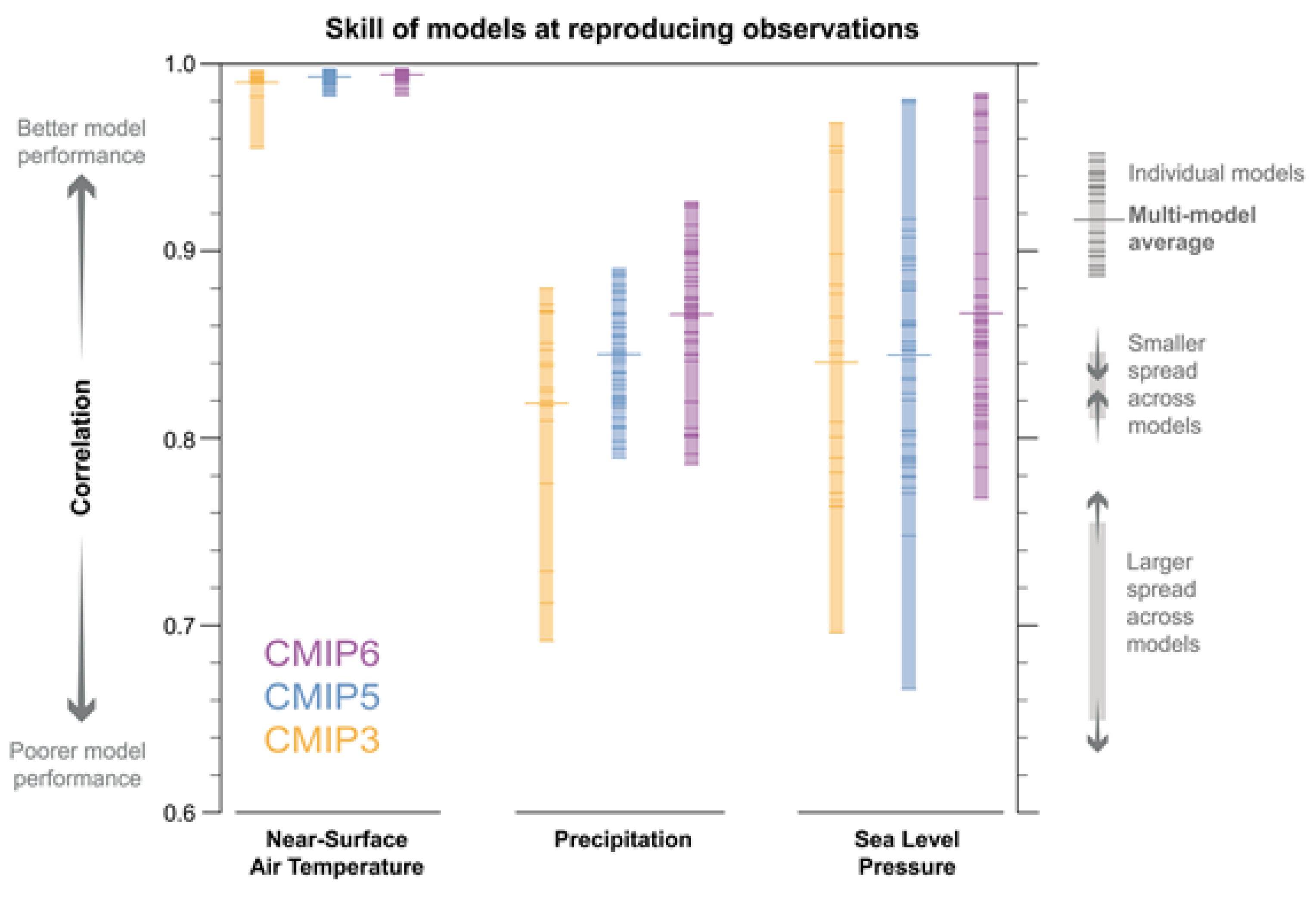
Figure 2.
Climate System Indicators and Feedback Mechanisms. Adapted from IPCC (2001).
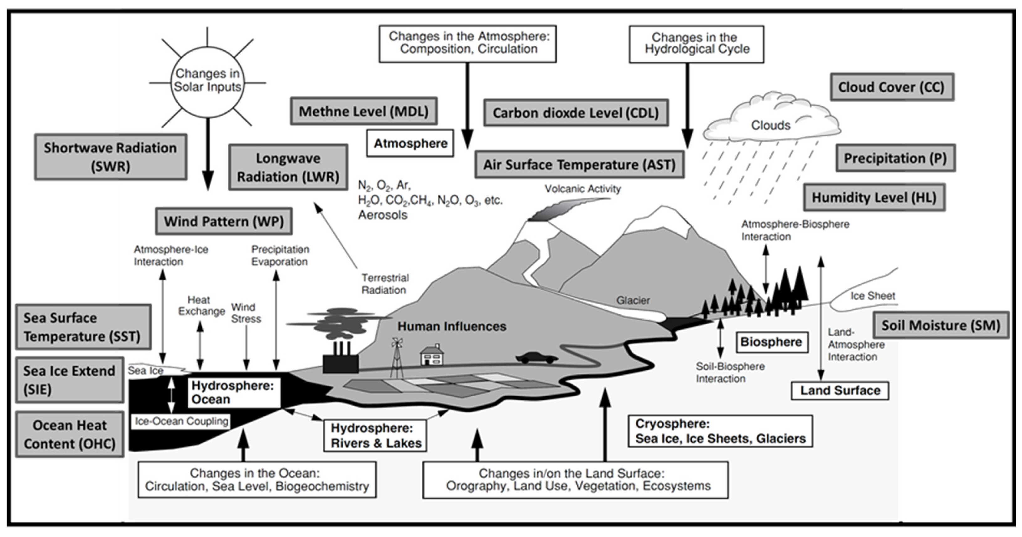
Figure 3.
Propagation of “Statistical-Induced Uncertainties” Through Pre- and Post-Processing Stages in Climate Modeling. Uncertainties in Data acquisition and collection ( UD), Statistical Induced Uncertainties in Input Pre-Processing Data (USIU-IN), Uncertainties in Input Pre-Processing Physics-Driven Models (UPDM), Uncertainties in Output Post-Processing Data (USIU-OUT).
UD), Statistical Induced Uncertainties in Input Pre-Processing Data (USIU-IN), Uncertainties in Input Pre-Processing Physics-Driven Models (UPDM), Uncertainties in Output Post-Processing Data (USIU-OUT).
Figure 3.
Propagation of “Statistical-Induced Uncertainties” Through Pre- and Post-Processing Stages in Climate Modeling. Uncertainties in Data acquisition and collection (UD), Statistical Induced Uncertainties in Input Pre-Processing Data (USIU-IN), Uncertainties in Input Pre-Processing Physics-Driven Models (UPDM), Uncertainties in Output Post-Processing Data (USIU-OUT).
UD), Statistical Induced Uncertainties in Input Pre-Processing Data (USIU-IN), Uncertainties in Input Pre-Processing Physics-Driven Models (UPDM), Uncertainties in Output Post-Processing Data (USIU-OUT).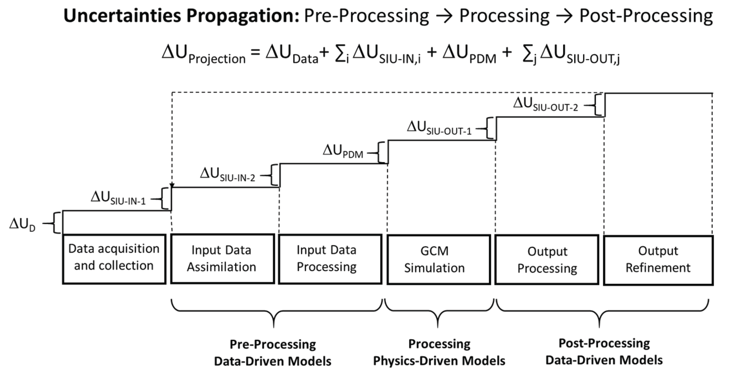
Disclaimer/Publisher’s Note: The statements, opinions and data contained in all publications are solely those of the individual author(s) and contributor(s) and not of MDPI and/or the editor(s). MDPI and/or the editor(s) disclaim responsibility for any injury to people or property resulting from any ideas, methods, instructions or products referred to in the content. |
© 2025 by the authors. Licensee MDPI, Basel, Switzerland. This article is an open access article distributed under the terms and conditions of the Creative Commons Attribution (CC BY) license (http://creativecommons.org/licenses/by/4.0/).
Copyright: This open access article is published under a Creative Commons CC BY 4.0 license, which permit the free download, distribution, and reuse, provided that the author and preprint are cited in any reuse.


