
Submitted:
27 November 2025
Posted:
27 November 2025
You are already at the latest version
Abstract
Two main perspectives exist regarding the interaction between fiscal deficits and expansionary monetary policy. The first perspective argues that fiscal deficits raise interest rates, thereby increasing interest payments and complicating monetary stabilization efforts. The second posits that expansionary monetary policy enhances nominal GDP growth, which in turn reduces the government debt-to-GDP ratio and strengthens the fiscal position. Using panel data from the IMF World Economic Outlook covering advanced economies between 1980 and 2025, this study empirically evaluates which perspective is more consistent with observed data, while accounting for the dynamics of tax revenues, government expenditures, interest rates, and nominal GDP growth. Empirical evidence indicates that moderate monetary expansion—raising nominal GDP—tends to stabilize budget deficits, as government revenues generally outpace expenditures and interest rates do not increase proportionally with nominal growth. These results are further illustrated through case studies of Greece, Italy, Portugal, Spain, Japan, the United Kingdom, and the United States.
Keywords:
monetary policy
; fiscal conditions
; interest rates
; nominal growth
1. Introduction
Two main perspectives characterize the debate on the relationship between fiscal deficits and expansionary monetary policy (Greenlaw et al., 2013). The first argues that fiscal deficits raise interest rates, thereby increasing interest payments and complicating monetary policy’s price stabilization efforts.
The second contends that expansionary monetary policy enhances nominal growth, reduces the government debt-to-GDP ratio, and thereby improves fiscal sustainability.
To assess fiscal deficits, it is crucial to examine the following relationships:
- The relationship between government revenue, nominal GDP, and the inflation rate.
- The relationship between government expenditure, nominal GDP, and the inflation rate.
- The relationship between the interest rate and the nominal growth rate
A budget deficit narrows when government revenues grow faster than expenditures. When , the risk of an unsustainable debt-to-GDP ratio remains low, and fiscal imbalances become less concerning. Recent empirical studies support the empirical regularity of (Blanchard, 2023; Mauro & Zhou, 2020; Checherita-Westphal & Semeano, 2020).
While previous research (Greenlaw et al., 2013) focused on the central bank’s financial position, this paper emphasizes the government’s fiscal situation. We utilize IMF panel data covering 41 countries over 45 years, examining government revenue, government expenditure, g, and r.
Our findings strongly suggest that moderate monetary expansion stabilizes budget deficits, supporting the second perspective. After presenting the general panel-data results, we examine fiscal trends in Greece, Italy, Portugal, Spain, Japan, the United Kingdom, and the United States. The first four countries are noted for challenging fiscal positions. Japan is often cited as fiscally vulnerable, yet no major fiscal crisis has materialized, while the United Kingdom and the United States, with significant financial centers, are highly sensitive to international market conditions.
2. Relationship Between Budget Situation and Monetary Policy
2.1. Relations of Budget Data and Nominal GDP
Let government debt be , net government debt be , the primary budget balance be PB = E − T, the budget balance be B = E − T + interestpayments, government expenditure excluding interest payments be E, government expenditure including interest payments be ER, tax revenue be T, nominal GDP be Y, and the interest rate be r.
Government debt evolves according to
Thus, the period-to-period increase in the government debt, , is
Differentiating the debt-to-GDP ratio, the growth rate of is
Noting and , we obtain
Equation (2) is the basic identity used throughout the paper. Stabilization of the debt-to-GDP ratio requires that
2.2. Relations between Fiscal Stability and Monetary Policy
This paper examines how monetary expansion affects fiscal stability by focusing on the behavior of
Monetary expansion is proxied by nominal GDP growth and increases in the consumer price index (CPI). We discuss the proxy variables latter.
2. Dataset
We collected annual data on ND, PB = E − T, the budget balance B = E – T + interest payments, E(excluding interest payments), .
Interest payments are calculated as the difference between the overall budget deficit and the primary deficit. The economy-wide implied interest rate is calculated as interest payments divided by the previous year’s government debt. Although actual coupon rates vary across instruments, this measure provides a useful proxy for the average cost of government borrowing.
Data are sourced from the IMF World Economic Outlook database and cover 41 advanced economies for 1980–2025, including IMF estimates for 2024–2025. The IMF definition of government employed here is general government, comprising central government, local government, and social security funds. Observations are included only when all required variables are available. However, data availability varies across countries, resulting in an unbalanced panel dataset.
2.1. Data Checks and Exclusions
We verified the computed by comparing it with nominal GDP growth and CPI growth; the comparison is reported in Figure 1. While most observations align, some series display volatility due to data revisions or very small net debt denominators (ND).
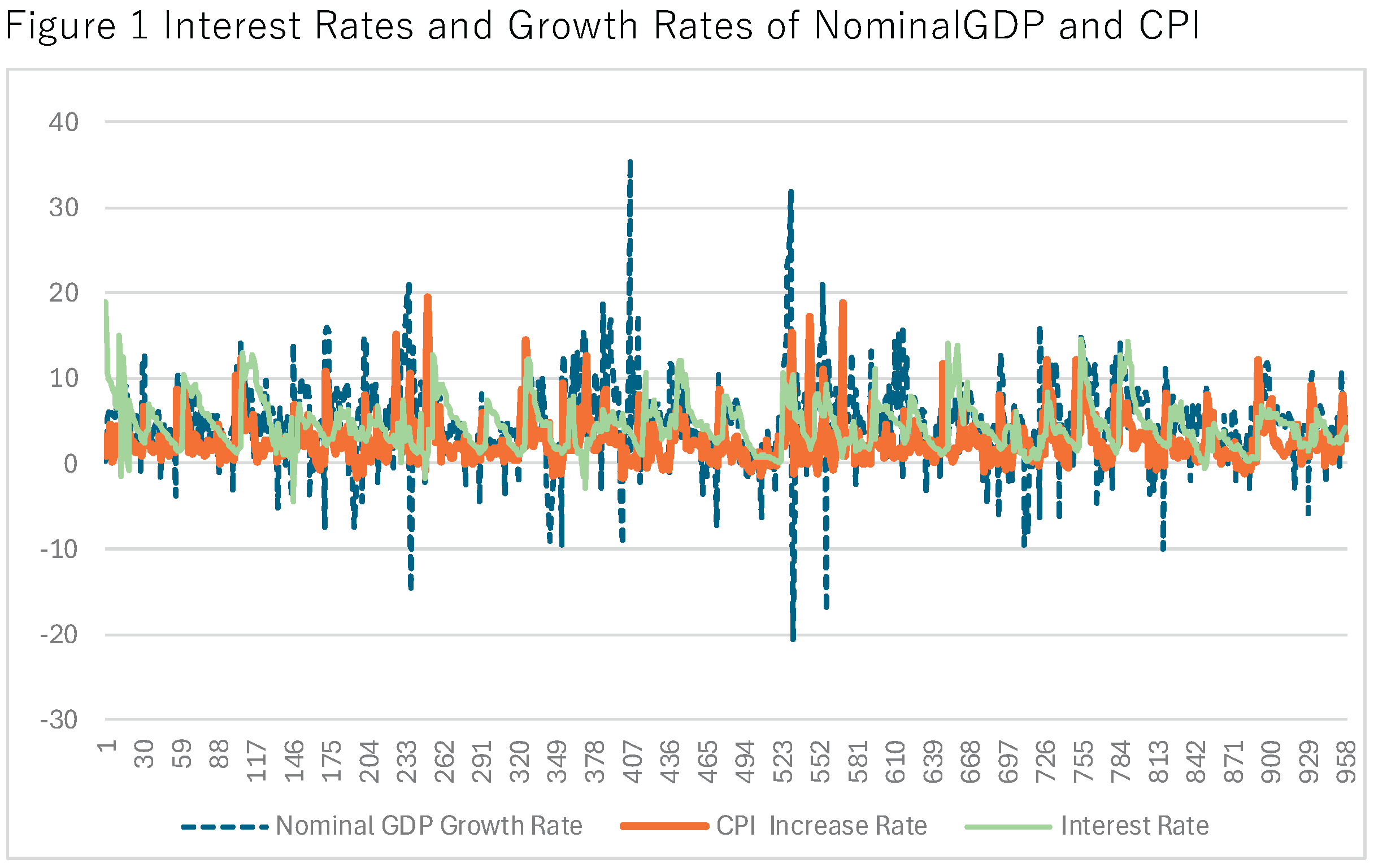
To exclude episodes of fiscal collapse or measurement unreliability, observations with annual CPI growth exceeding 20% or consecutive two-year CPI growth exceeding 15%, and observations with nominal interest rates above 20%, were removed. Monetary expansion is treated as increasing nominal GDP and CPI; monetary contraction has the opposite effect. We analyze how these channels affect net government debt.
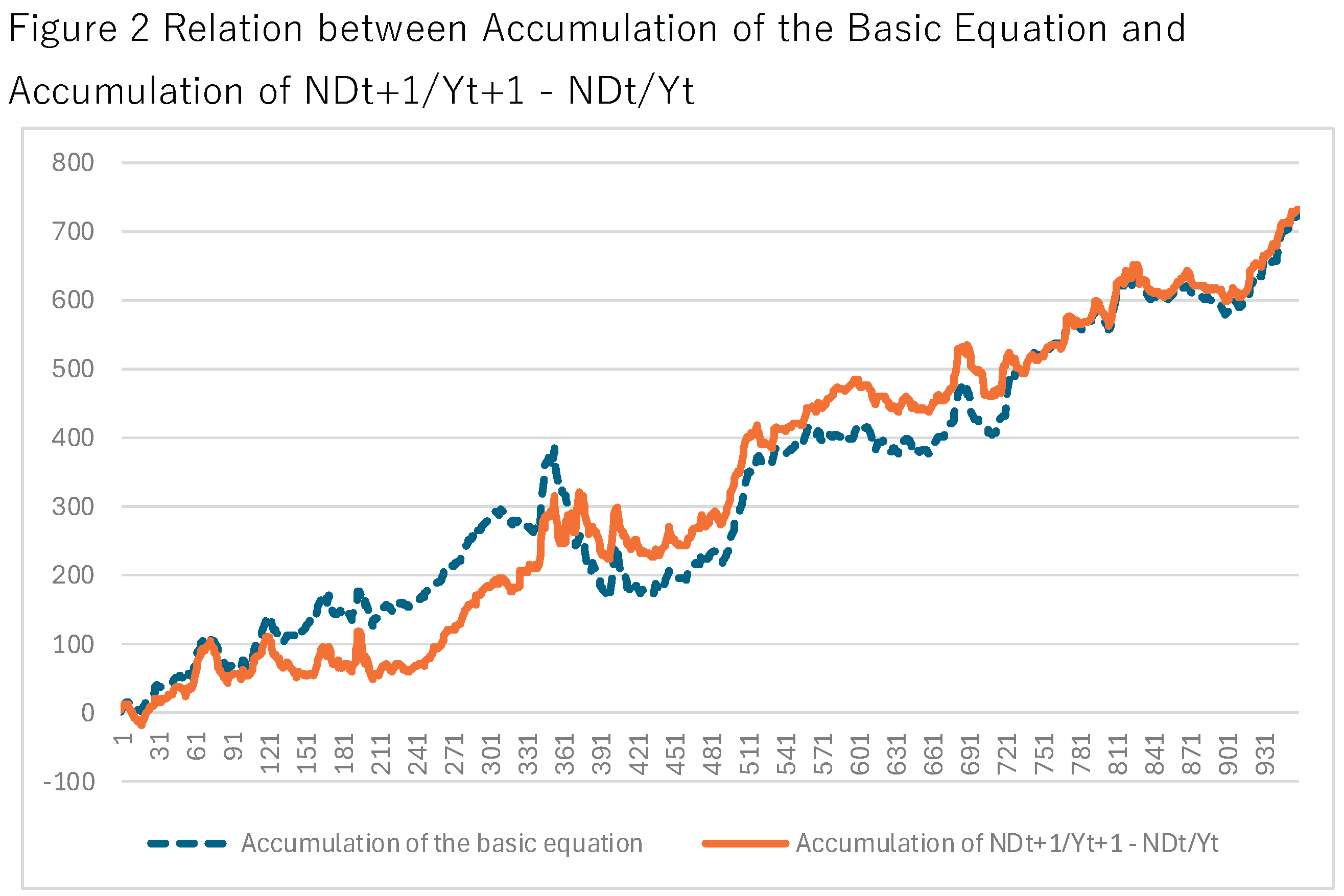
Because is volatile, we compute it as and compare it with. Both series remain volatile in annual frequency; accordingly, we compare their accumulated values. Figure 2 shows that accumulated series move in similar directions.
2.2. Descriptive Statistics
Table 1 presents descriptive statistics and definitions for all variables.
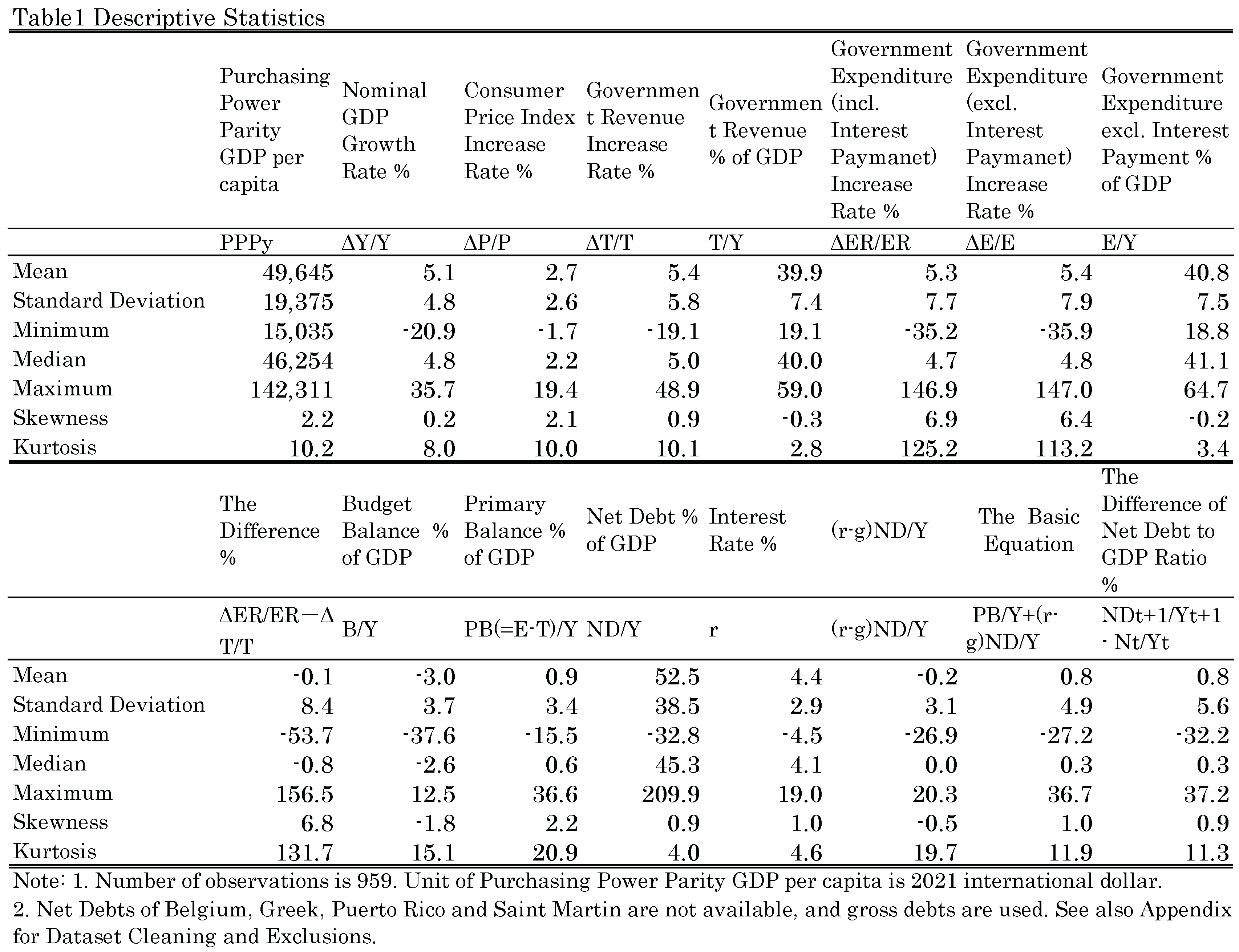
- PPP (Purchasing Power Parity) GDP per capita (2021 international dollars): mean $49,645; minimum $15,035; maximum $142,311, indicating the sample is concentrated in advanced economies.
- CPI inflation: mean 2.7%; minimum −1.7%; maximum 19.4%.
- Nominal GDP growth: mean 5.1%.
- Nominal interest rate: mean 4.4%; the pooled sample therefore exhibits a negative average r %#x2212; g.
The relationship between nominal growth and interest rates has been the subject of extensive debate. Mauro and Zhou (2020) document that, contrary to traditional assumptions, negative differentials have become increasingly common since the 2008 global financial crisis, based on a long historical sample. Nevertheless, marginal government borrowing costs can spike sharply, particularly immediately prior to default. Because the present study excludes high-interest episodes, it focuses on relatively stable periods in which governments exercise substantial control over inflation and interest-rate volatility.
3. Estimation
We estimate the effects of monetary policy on the following dependent variables: the growth rate of government expenditure ; the growth rate of government revenue ; the difference between these two growth rates ; the nominal interest rate ; and the expression ; Monetary policy is captured by the nominal GDP growth rate and the CPI inflation rate .
Figure 3 plots nominal GDP growth against government revenue growth. The horizontal axis represents nominal GDP growth, and the vertical axis represents government revenue growth. As expected, higher nominal GDP growth is generally associated with faster growth in government revenue. The pooled regression line exhibits a positive slope of 0.931. Under a progressive tax system, one would typically anticipate a slope exceeding unity, since nominal wage increases tend to move taxpayers into higher income brackets. The observed slope of 0.931 therefore suggests that, on average, countries adjust tax parameters or otherwise mitigate inflation-induced bracket creep.
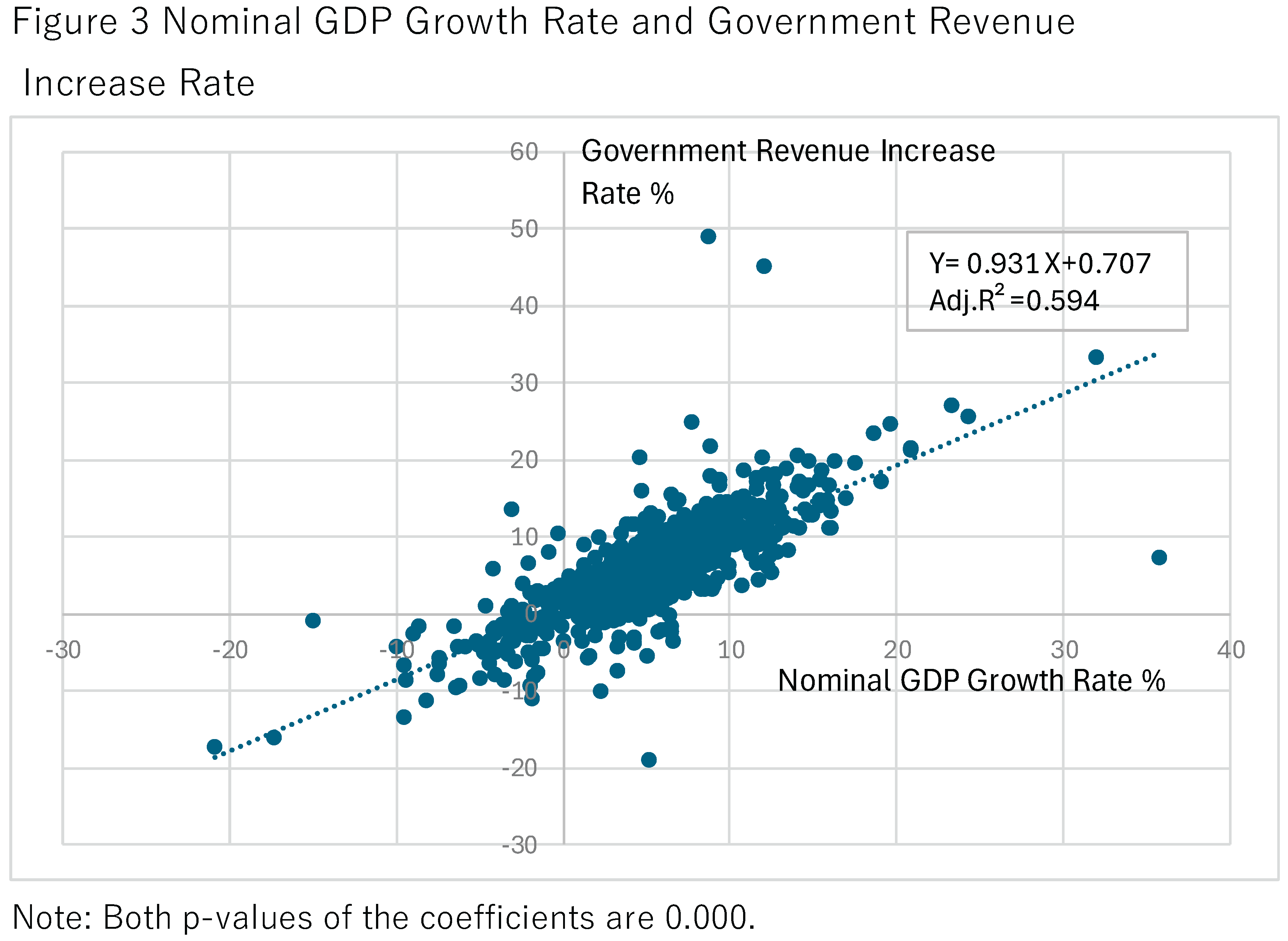
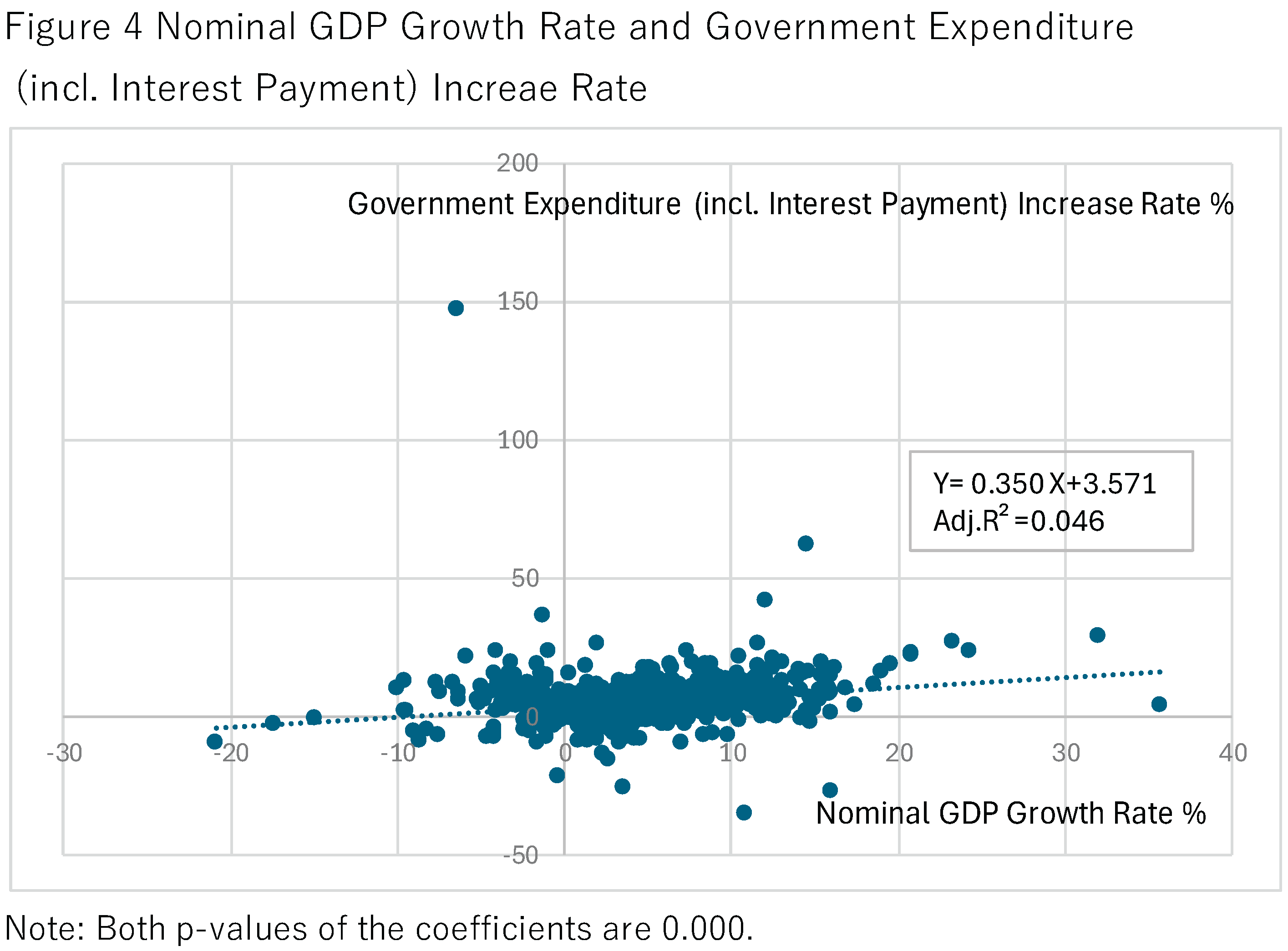
Figure 4 depicts nominal GDP growth against government expenditure growth (including interest payments). When nominal GDP rises, prices, real incomes, and interest rates also tend to increase, raising the prices of goods and services purchased by the government, the wages of public employees, and interest payments on government debt. Accordingly, government expenditure growth typically increases with nominal GDP growth. The pooled regression slope is modest, at 0.350. The difference between the revenue slope (0.931) and the expenditure slope (0.350) implies that budget deficits tend to narrow as nominal GDP rises.
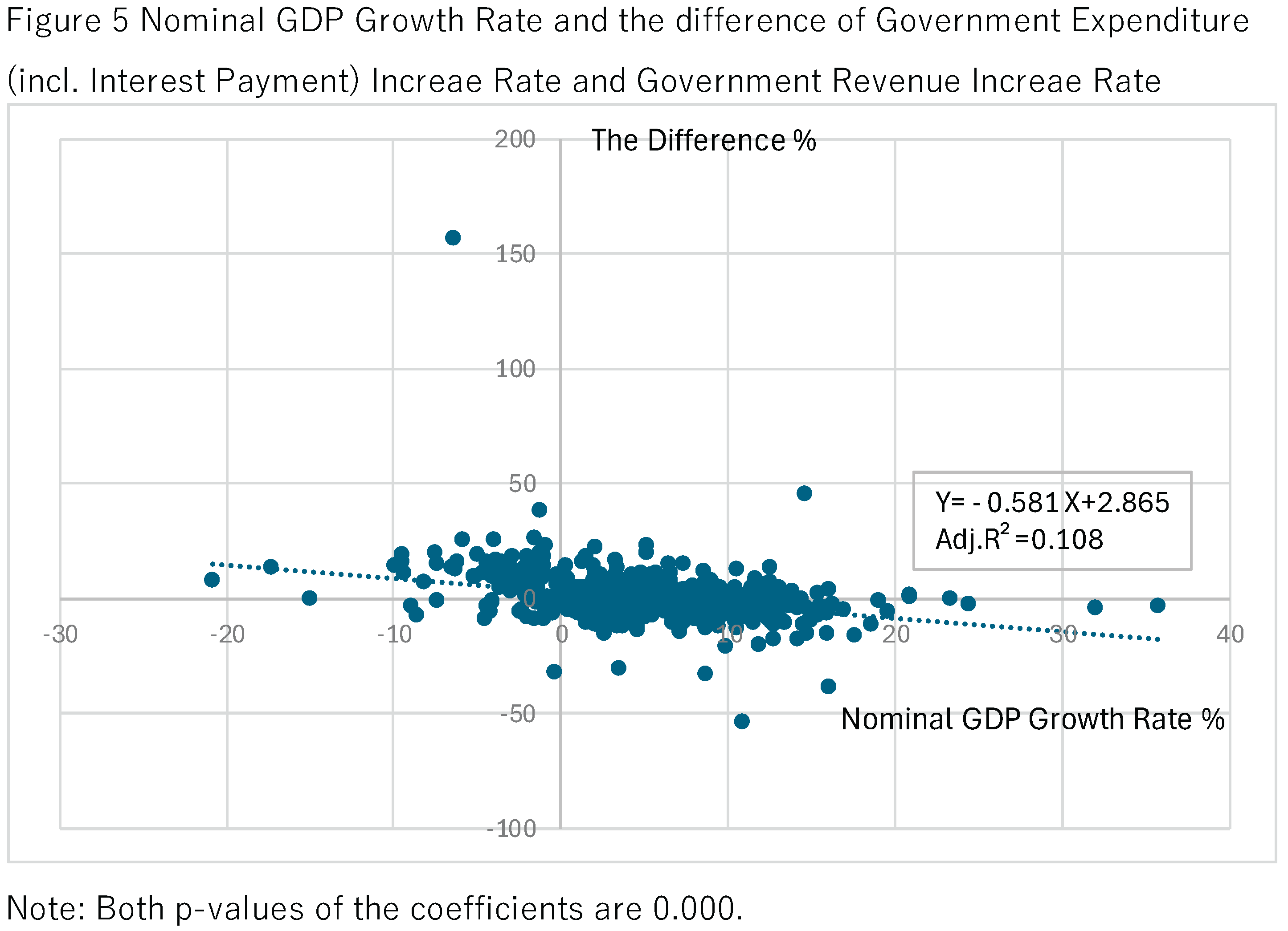
Figure 5 displays the relationship between nominal GDP growth and the growth differential (expenditure minus revenue). The pooled slope of −0.581 confirms that higher nominal GDP growth tends to reduce the fiscal gap.
Results obtained using CPI inflation in place of nominal GDP growth are qualitatively similar. Because these CPI-based figures display nearly identical patterns, they are omitted here; subsequent sections present the formal estimation results.
3.1. Model Selection
The empirical analysis employs country-by-year panel data. We estimate both a country fixed-effects model, which removes time-invariant country heterogeneity, and a two-way fixed-effects model that includes country and year fixed effects to control for common temporal shocks. In all specifications we compute cluster-robust standard errors at the country level to account for within-country serial correlation and heteroskedasticity, thereby improving the reliability of inference.
Model selection proceeded by estimating fixed-effects and random-effects specifications and applying Hausman tests to assess whether country-specific effects are correlated with the regressors. The Hausman tests favor fixed-effects, and consequently the two-way (country and year) fixed-effects specification is adopted for the reported results.
3.2. Estimation Results
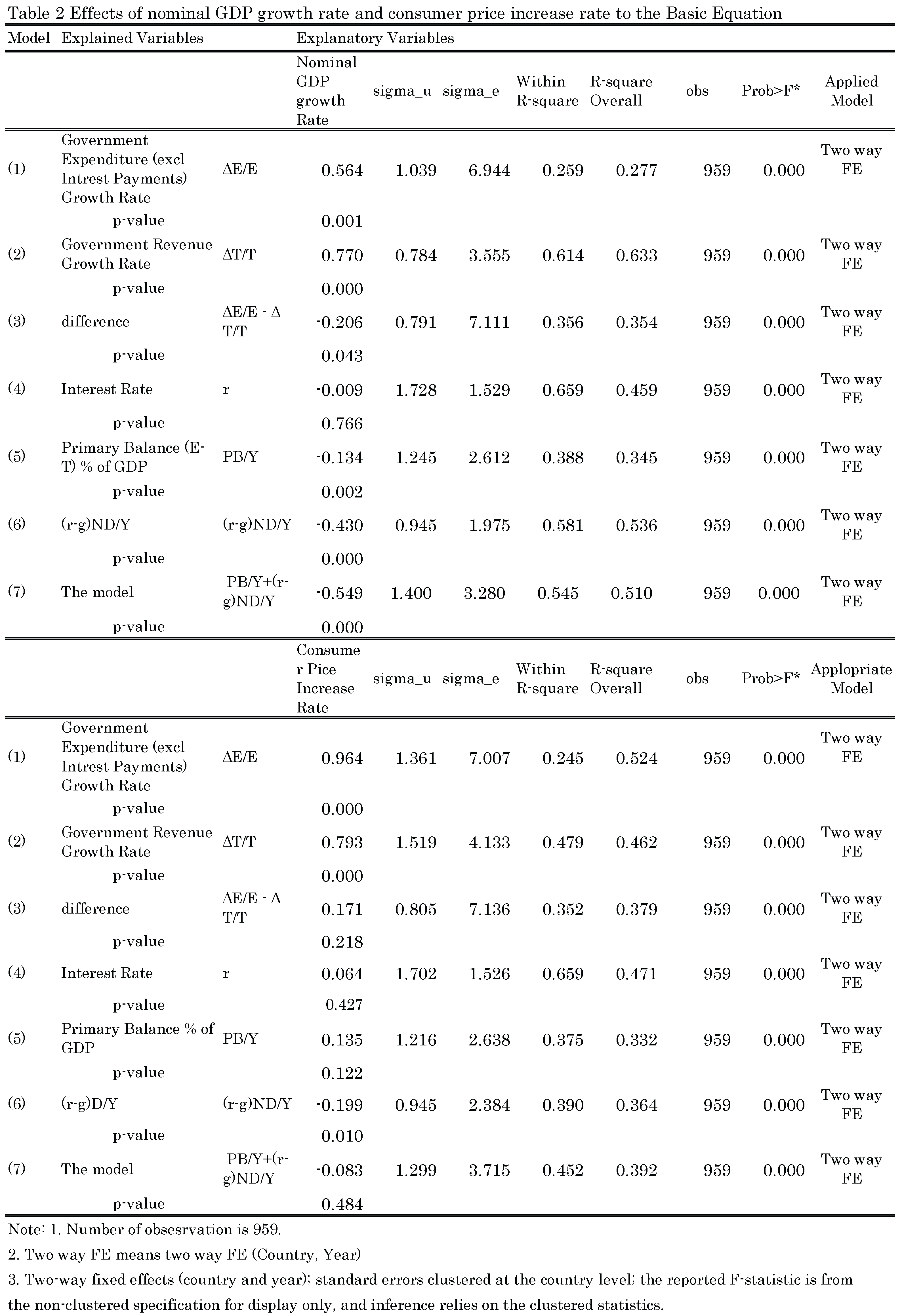
Table 2 reports estimated coefficients for models using nominal GDP growth and consumer price increase rate as the monetary-policy proxy1.
A possible concern is that nominal GDP growth and CPI inflation may be influenced by factors other than monetary policy, making them imperfect proxies. However, McCandless and Weber (1995), using data from 110 countries over 30 years, demonstrate strong positive correlations between money growth and inflation, and—within the OECD subsample—positive correlations between money growth and real GDP. Therefore, nominal GDP and CPI inflation are reasonable indicators of monetary policy stance in this context2.
3.3. Effects of Nominal GDP Growth (Models 1–7)
- Model (1): A one percentage point increase in nominal GDP growth is associated with a 0.564 percentage point increase in government expenditure growth .
- Model (2): A one percentage point increase in nominal GDP growth corresponds to 0.770 percentage point increase in government revenue growth . The estimated coefficient of 0.770 is consistent with the interpretation that many countries adjust tax parameters to limit bracket creep induced by inflation.
- Model (3): A one percentage point increase in nominal GDP growth reduces the gap between government expenditure growth and government revenue growth by 0.206 percentage points, consistent with Models (1) and (2) and implying that higher nominal growth reduces the budget deficit3.
- Model (4): Nominal GDP growth tends to reduce the nominal interest rate, but the estimated effect is small (0.009) and not statistically significant4.
- Model (5): Nominal GDP growth improves the primary balance ratio , consistent with the inference from Model (3).
- Model (6): Nominal GDP growth mitigates the term, meaning nominal growth exceeds interest rates as we discussed before5.
- Model (7): Consolidating the components in Models (5) and (6), nominal GDP growth reduces , a reduction in .
Most coefficients reported are statistically significant at conventional levels (1% or 5%), except in Model (4) explicitly noted.
3.4. Effects of CPI Growth (Models 1–7)
When CPI growth replaces nominal GDP growth as the monetary-policy proxy, results are not necessarily similar.
- Model (1): A one percentage point increase in CPI is linked to a 0.964 percentage point increase in government expenditure growth, indicating that a one percent rise in prices is nearly matched by a one percent increase in government spending.
- Model (2): A one percentage point increase in CPI is positively related to a 0.793 percentage point increase in government revenue growth.
- Model (3): A one percentage point increase in CPI is associated with a 0.171 percentage point increase in the expenditure minus revenue growth differential, implying increase in the budget deficit; however, this coefficient is very small and statistically insignificant.
- Model (4): A one percentage point increase in CPI raises the nominal interest rate by 0.064 percentage points, consistent with a Fisher-type effect; the coefficient is small and statistically insignificant in the short run and may be more relevant over longer horizons6.
- Model (5): CPI growth is estimated to deteriorate the primary balance ratio , and this coefficient is statistically insignificant at the 5% level, aligning with the (weak) findings of Model (3).
- Model (6): CPI growth mitigates the.
- Model (7): CPI growth’s net effect on is statistically insignificant; components increase and decrease different parts of the equation, resulting in an ambiguous net effect in this specification.
3.5. Brief Summary
Using panel data from the IMF World Economic Outlook, the empirical results indicate that nominal GDP growth reduces the debt-to-GDP ratio, whereas CPI inflation alone shows no clear relationship with the debt ratio—suggesting that real growth plays a crucial role in fiscal stabilization. When monetary expansion stimulates both nominal and real GDP growth, the debt-to-GDP ratio tends to decline; when it merely raises prices, the ratio does not necessarily improve.
We also find that nominal GDP growth is positively associated with the output gap in pooled regressions, with the coefficient statistically significant at the 1% level. This finding is consistent with a Phillips-curve relationship within the pooled sample: nominal GDP growth increases the output gap and thereby contributes to debt stabilization.
Overall, moderate monetary expansion stabilizes fiscal positions, as government revenue rises more rapidly than expenditure, while interest rates increase by less than nominal GDP growth. In contrast, price-only inflation fails to improve fiscal balances because energy-price-driven CPI increases typically deteriorate the terms of trade for most advanced economies, depress output and tax revenues, and thereby widen budget deficits.
4. Case Studies
This section examines the fiscal dynamics of seven advanced economies: Italy, Greece, Portugal, Spain, Japan, the United Kingdom, and the United States. The Southern European countries—namely Italy, Greece, Portugal, and Spain—have faced persistent fiscal vulnerabilities, often exacerbated by low growth and elevated sovereign risk premia. Japan represents a distinct case, characterized by prolonged deflationary pressures and unconventional monetary policy responses. The United Kingdom and the United States, while possessing relatively flexible fiscal frameworks, remain highly sensitive to global financial market fluctuations and external shocks.
(1) Greece
In October 2009, a change in government occurred in Greece. Under the newly elected administration, it was revealed that the previous government had significantly understated the fiscal deficit. Contrary to the reported figure of approximately 4% of GDP, the actual deficit was found to be 13%. In response, the new government announced a three-year fiscal consolidation plan aimed at reducing the deficit to below 2.8% of GDP.
However, concerns over sovereign default triggered a sharp deterioration in financial markets: yields on Greek government bonds surged, equity prices declined, and the euro depreciated7. On April 23, 2010, Greece formally requested financial assistance from the International Monetary Fund (IMF), the European Commission, and the European Central Bank (ECB). As a condition for receiving support, Greece committed to implementing austerity measures8.
While many analyses attribute the Greek crisis primarily to unsustainable fiscal policy, this study emphasizes the interaction between nominal GDP growth and fiscal dynamics. As previously discussed, the debt-to-GDP ratio is influenced by the nominal GDP growth rate, the primary balance-to-GDP ratio , and the term . These components are captured in the debt dynamics equation: ,where variable definitions are identical to those in the proceeding section.
Figure 6 illustrates the evolution of these variables. The global financial crisis of 2009 severely impacted the Greek economy, with nominal GDP growth falling from over 5% to −1.8%, and further to −9.0% in 2011. Following 2009, turned negative, indicating a reduction in the primary deficit. However, the term rose to over 20%, exacerbating the overall deficit9.
In 2020, nominal GDP growth declined again, while temporarily increased. Subsequently, both and declined as nominal growth recovered. The sharp increase in government expenditure during this period was largely attributable to the COVID-19 pandemic.
Despite improvements in due to austerity measures, the debt-to-GDP ratio did not begin to decline until 2020. It only fell meaningfully after 2021, coinciding with a recovery in nominal GDP growth. The inverse relationship between nominal GDP growth and before and after 2009 underscores the critical role of nominal growth in reducing fiscal deficits.
The austerity program imposed substantial social costs. The unemployment rate surged to 27.5% in 2013, a level comparable to that experienced during the Great Depression of the 1930s.
(2) Italy
For the remaining countries, we focus on the dynamics of nominal GDP and fiscal indicators rather than detailed historical accounts.
In Italy, nominal GDP growth contracted by −3.6% in 2009 and −7.4% in 2020. Following these contractions, turned negative or declined, while rose to 6.5% in 2012. After 2020, however, fell to −10.9% in 2021, indicating a fiscal improvement.
Figure 7 presents these dynamics. Despite the implementation of austerity measures, the debt-to-GDP ratio did not decline. The ineffectiveness of austerity is attributed to the contraction in nominal GDP growth, which increased the term. Conversely, the recovery in nominal growth contributed to a reduction in the debt ratio.
Critics may argue that monetary tightening was necessary to contain inflation, thereby justifying the decline in nominal growth. However, as shown in Figure 6 and Figure 7, consumer price inflation rates in Greece were 4.7% and 3.1% in 2010 and 2011, respectively, while Italy’s were 2.9% and 3.3% in 2011 and 2012. Meanwhile, unemployment rates increased to 27.5% in Greece and 12.8% in Italy. This evidence raises questions about the necessity of austerity.
Even if higher nominal growth could have supported these economies, monetary policy was controlled by the European Central Bank (ECB), limiting national discretion. The ECB’s policy stance differed markedly across crises: two-year nominal GDP annual growth rates in the euro area after the Global Financial Crisis (GFC) in 2009 and after the COVID-19 crisis were 2.8% and 8.8%, respectively, while monetary base growth rates were 2.3% and 26.7%10. These contrasts reflect different monetary policy responses.
Comparable fiscal dynamics are evident in Portugal and Spain, though their figures are omitted here for brevity.
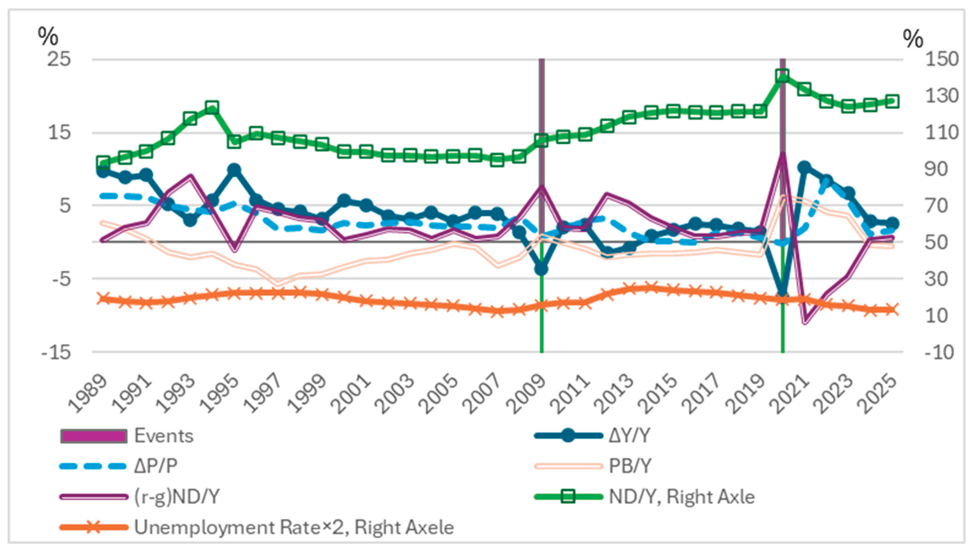
(3) Japan
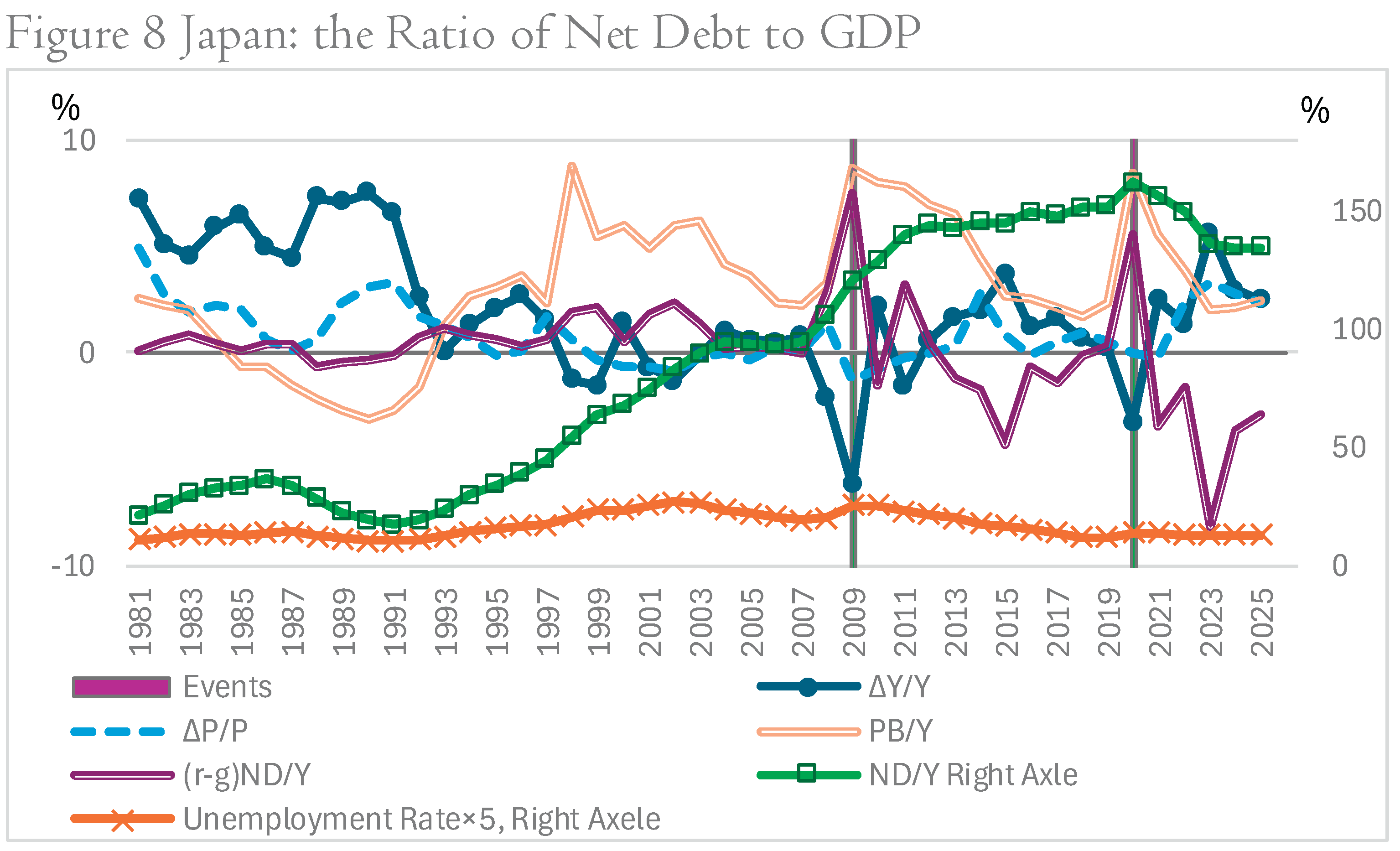
Japan exhibits similar contrastive movements between nominal GDP growth and as observed in Greece and Italy. However, Japan maintained a higher than the other countries, which contributed to a relatively higher . Nevertheless, post-2020 nominal GDP growth ultimately led to a reduction in as nominal GDP grows[11]. Nominal GDP growth contributes to decline of in the latter half of 1980s, and stopping upward trend of the ratio after 2011. Unemployment rate increased as nominal GDP growth declined from 1990s to the early 2000s and it decreased as nominal GDP growth recovered after 2012 except Covid-19 period. Figure 8 presents these trends.
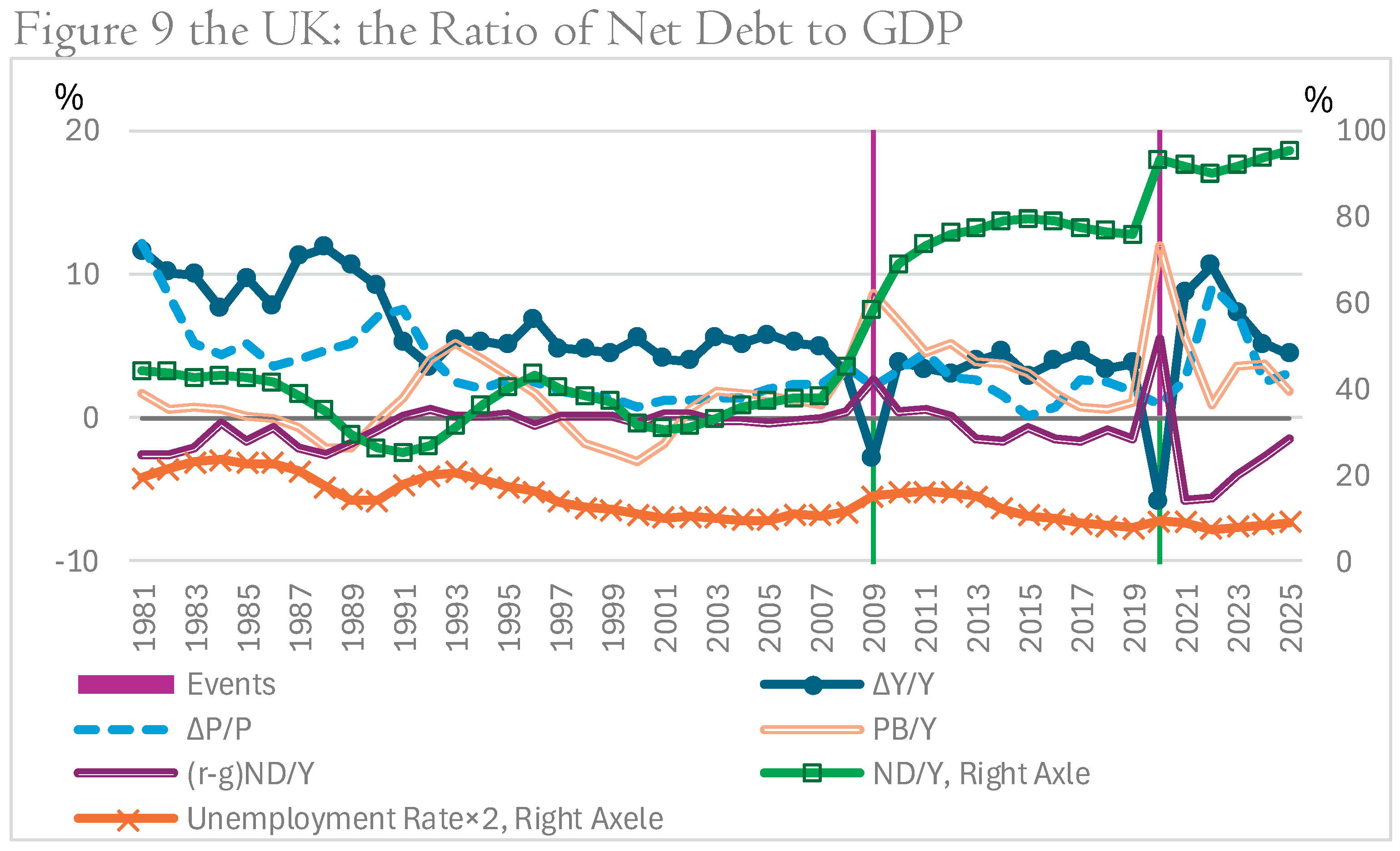
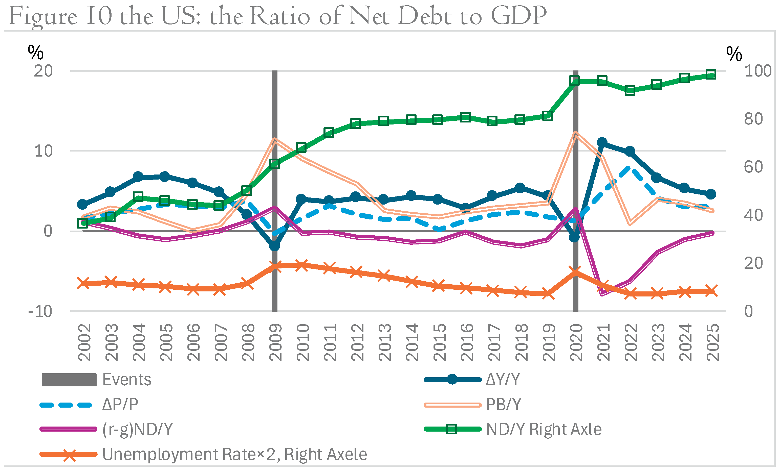
(4) the United Kingdom and the United States
Both countries show patterns in which post–2020 nominal GDP growth contributed to declines in ; their large and globally integrated financial sectors render these economies sensitive to international market conditions and risk premia, but the dominant role of nominal growth in improving debt ratios is evident in the observed trajectories.
Figure 9 and Figure 10 depicts the relevant data.
5. Conclusions
Using IMF panel data for advanced economies, the empirical analysis demonstrates that nominal GDP growth materially contributes to fiscal consolidation. Moderate monetary expansion that raises nominal GDP is associated with reductions in the debt-to-GDP ratio, supporting the second perspective introduced earlier. CPI inflation alone yields more ambiguous effects: when inflation accompanies both real and nominal GDP growth, fiscal outcomes improve; when inflation occurs without corresponding nominal growth, debt ratios may not decline.
Across case studies of Italy, Greece, Portugal, Spain, Japan, the United Kingdom, and the United States, nominal GDP growth improves fiscal and employment conditions, even if it modestly increases inflation. Nevertheless, a moderate inflation rate of a few percent is far preferable to an unemployment rate approaching 30%.
Some may argue that nominal GDP growth merely reflects cyclical fluctuations. While this is partly true, the contrasting nominal GDP growth rates of the euro area following the Global Financial Crisis and after the COVID-19 crisis highlight the importance of monetary policy differences, as discussed in the Italian case.
This analysis omits episodes of extreme inflation or severe sovereign distress by design; results therefore apply to relatively stable periods during which governments retain substantial control over inflation and interest-rate volatility.
6. Appendix for Dataset Cleaning and Exclusions
Taiwan and Singapore are excluded due to missing primary balance data. Austria, Belgium, Hong Kong, Korea, Puerto Rico, and San Marino lack net debt data, so gross debt is used instead. Interest rates in these countries remained stable despite this substitution, likely because government-held financial assets are limited. Macao is excluded as it lacks both net and gross debt data.
Denmark, Finland, Hong Kong, Ireland, and Korea are excluded due to negative interest rates. Norway is excluded because calculated interest rates were anomalously high (16–55%) during 1981–1995.
Interest rates are calculated as net interest payments divided by net government debt. When net interest payments are negative (i.e., governments earn more interest than they pay) while net debt remains positive, the resulting interest rate is negative and considered non-informative, as it reflects idiosyncratic factors rather than genuine financing costs. Such observations are excluded.
Interest rates in Sweden were negative for 2019–2021, reflecting global ultra-low interest conditions; these data are retained. As a result, the final sample comprises 37 countries.
END
We appreciate your kindness for giving us granting a waiver of the submission fee of this paper.
References
- Amadeo, Kimberly, “The Balance — Greek Debt Crisis: Summary, Causes, Timeline, Outlook —,” Updated on , 2019, “https://www.thebalancemoney.com/what-is-the-greece-debt-crisis-3305525. 14 December.
- Blanchard, Olivier (2023). Fiscal Policy under Low Interest Rates, The MIT Press.
- Checherita-Westphal, C. D. , & Semeano, J. D. (2020). “Interest rate-growth differentials on government debt: an empirical investigation for the euro area” European Central Bank.
- Gagliardone, Luca, Mark Gertler, Simone Lenzu, and Joris Tielens (2023), “Anatomy of the Phillips Curve:Micro Evidence and Macro Implications,” Working Paper 31382, National Bureau of Economic Research.
- Greenlaw, D, J. D. Hamilton, P. Hooper, and F.S. Mishkin (2013), “Crunch Time: Fiscal Crises and the Role of Monetary Policy,” Working Paper 19297. National Bureau of Economic Research.
- Mauro, M. P. , & Zhou, J. (2020). “r minus g negative: Can we sleep more soundly?”. International Monetary Fund.
- McCandless, George T. Jr. and Warren E. Weber (1995), “Some Monetary Facts,” Quarterly Review, Federal Reserve Bank of Minneapolis, Summer.
Figure 6.
Greece: the Ratio of Gross Debt to GDP.
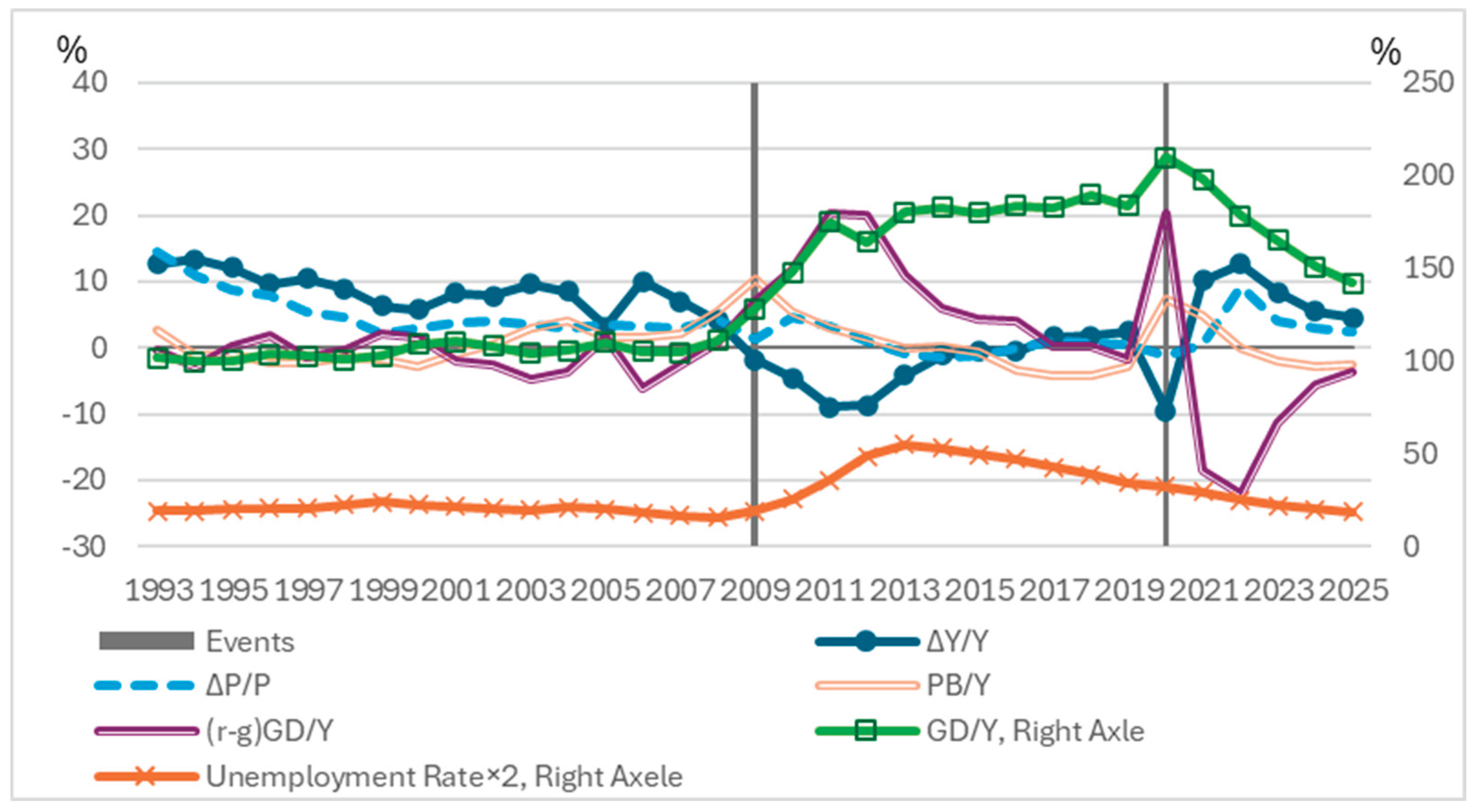
Figure 7.
Italy: the Ratio of Net Debt to GDP.
| [1] | We refrain from simultaneously including the GDP growth rate and the consumer price inflation rate in the models, since nominal GDP growth equals the sum of real GDP growth and the GDP deflator growth, and nominal GDP growth is correlated with the CPI inflation rate. Although the correlation coefficient between the two variables (0.5196) indicates that multicollinearity is not statistically significant, we exclude their joint estimation in light of the theoretical interdependence between them. |
| [2] | Year-specific effects are excluded because the estimation employs a two-way fixed model. For example, the global financial crisis of 2009 lowered nominal GDP growth rates, weakened fiscal positions, and thereby induced a correlation between nominal GDP and fiscal variables. This correlation, however, is absorbed by the year-specific effect. Accordingly, the estimated relationship between nominal GDP and fiscal positions can be interpreted as relatively unbiased with respect to time-specific shocks. |
| [3] | The coefficients reported in Table 2 differ from the simple OLS slopes shown in Figures 3–5 because Figures 3–5 employ expenditure measures that include interest payments and are estimated using pooled OLS, whereas Table 2 presents for a two-way fixed-effect estimates. |
| [4] | The interest rate used here is computed as interest payments divided by the previous year’s government debt, representing an average rate on government bonds issued in prior years. Therefore, this rate is not immediately affected by changes in nominal growth or inflation. |
| [5] | The term (r − g) is largely driven by g, which makes the estimation results intuitive; however, this also distorts the coefficient and its p-value. That said, the coefficient on r in Model (4) is small, confirming that increases in g do not lead to a substantial rise in r. |
| [6] | See also note 4. |
| [7] | The interest rate paid by the government did not surge, it remained around 4.5% in 2009 and 2010. This is because the rate reflects average yields on previously issued bonds. |
| [8] | Regarding the Greek Crisis, we primarily refer to Amadeo (2019). |
| [9] | Net debt data for Greece are unavailable: therefore, gross debt (GD) is used instead. |
| [10] | For nominal GDP: OECD Data Explorer, Annual GDP and components — expenditure approach, Euro area (20 countries). |
| [11] | The Japanese government holds substantial foreign assets, whose value increases when the yen depreciates. As a result, the effect of nominal GDP growth on net debt may be overstated. |
Disclaimer/Publisher’s Note: The statements, opinions and data contained in all publications are solely those of the individual author(s) and contributor(s) and not of MDPI and/or the editor(s). MDPI and/or the editor(s) disclaim responsibility for any injury to people or property resulting from any ideas, methods, instructions or products referred to in the content. |
© 2025 by the authors. Licensee MDPI, Basel, Switzerland. This article is an open access article distributed under the terms and conditions of the Creative Commons Attribution (CC BY) license (http://creativecommons.org/licenses/by/4.0/).
Copyright: This open access article is published under a Creative Commons CC BY 4.0 license, which permit the free download, distribution, and reuse, provided that the author and preprint are cited in any reuse.


