
Submitted:
26 November 2025
Posted:
27 November 2025
You are already at the latest version
Abstract
Urban and peri-urban agriculture (UA) plays an increasingly important role in pro-moting sustainable urban development, delivering socioeconomic, environmental, and educational benefits. However, UA is often associated with nutrient accumulation in soils, as vegetable-growing areas typically receive substantial inputs of organic and inorganic fertilizers. This study examines soil variability in two sections of an urban allotment garden subjected to long-term manure fertilisation for 12 or 16 years at ap-plication rates up to 10–12 kg m⁻² yr⁻¹. Surface soils were analysed for organic and in-organic carbon, total N, available P and K, pH, and elemental composition using port-able X-ray fluorescence (pXRF). Prolonged manure incorporation substantially in-creased soil fertility, evidenced by elevated soil organic carbon, total N, available K, and both total and available P. Marked shifts in mineral composition were also ob-served, including significant increases in total Ca, inorganic C (as calcium carbonate), Sr, and S. Despite the high manure inputs, no accumulation of potentially toxic ele-ments (PTEs) was detected. Nevertheless, pronounced heterogeneity was found among individual plots, reflecting differences in fertilisation intensity and management prac-tices. pXRF proved highly effective for identifying soil compositional changes and pre-dicting nutrient availability, highlighting its potential as a rapid diagnostic tool for precision agriculture management.
Keywords:
compost
; organic amendment
; potentially toxic element
; soil fertility
; soil organic carbon
; urban agriculture
1. Introduction
Urban and peri-urban agriculture (UA) plays an increasingly crucial role in urban development, not only by improving food availability and accessibility but also through its multidimensional contributions to sustainable urban growth, including socioeconomic, environmental, and educational benefits [1]. There are compelling reasons to promote the expansion of UA, such as responding to rapid urbanization, concerns about the impacts of conventional agriculture on climate change, and the need to address food security and accessibility issues [2].
As a more local food production system, UA brings food production closer to consumers, providing access to affordable and nutrient-rich foods, and consequently helping to mitigate the adverse effects associated with the prevailing long-distance food supply chains [2]. Urban agriculture (UA) is a rapidly expanding global practice—driven both by the pace of urban growth and by supportive policies in more developed countries. Municipal and regional governments often encourage UA by providing essential resources such as land, water, irrigation systems, and fencing, while requiring only minimal financial contributions from participating gardeners. In less developed countries, UA is often associated with low-input agriculture and limited productive means.
However, in developed or recently developed countries, UA is frequently linked to the accumulation of soil nutrients, as vegetable-growing soils receive large amounts of organic and inorganic fertilizers [3]. The high nutrient contents often originate from intensive fertilization practices using animal manures [3].
Organic farming (OF) practices are commonly adopted within UA systems. In organic vegetable production, due to the high nitrogen and potassium demands of crops, fertilization management requires external sources of these nutrients such as manures, compost, or organic amendments—preferably derived from OF systems—which are used as base fertilizers [4,5]. Although organic fertilizers can increase greenhouse gas (GHG) emissions, their net effect is a negative carbon balance, as they enhance soil carbon sequestration and reduce fossil fuel use associated with synthetic fertilizer production. Overall, while organic fertilizers pose challenges regarding GHG emissions, their multiple benefits justify careful consideration and strategic implementation in agricultural systems [6].
Manures not only recycle macro- and micronutrients back into the soil but also contribute significant amounts of organic matter and microorganisms [7]. Soil organic matter exerts profound physical (structure, aeration, water retention), chemical (nutrient retention), and biological (biodiversity, disease suppression, biomass) effects, thereby maintaining soil health and crop productivity [7,8].
While the advantages of manure use are well known, its mismanagement can lead to serious problems. This has prompted the European Union and other countries to implement restrictive regulations on its agricultural use, setting limits on application rates, conditions, and methods, primarily to prevent nitrate contamination of water resources, such as through the Nitrates Directive [9].
Despite the long-standing tradition and extensive knowledge of manure use in agriculture, a recent European Union report [7] highlights emerging research priorities that extend beyond the well-documented nitrogen-related adverse effects. These include additional impacts of manures and their derivatives on human health and the environment, such as soil fertility effects derived from manure management, the presence of microcontaminants (e.g., metals and pesticides), and the influence of manure processing on the biogeochemical cycle of phosphorus [7] (pp. 28–29).
Family or allotment gardens are a common UA typology in developed countries [10] and are expanding globally. In these systems, non-professional gardeners cultivate vegetables on small plots, following their own management criteria, albeit often within a set of shared regulations. These gardens are non-commercial in nature, and while organic practices are frequently adopted, certification processes are typically avoided to reduce costs. Organic amendments are commonly used without precise control—often without nutrient content analyses of either the materials applied or the soil itself.
A global issue in urban gardens is the presence of contaminants such as potentially toxic trace elements (PTEs) [11,12], which may eventually reach crops and pose health risks to humans [13]. Soil contamination in urban gardens can result from multiple sources, including nearby housing, road traffic, urban or industrial activities, as well as from the gardeners’ own practices, such as the use of fertilizers, waste materials, or pesticides [14,15].
A recent study indicates that organic residues and tillage practices often induce spatial heterogeneity in soil properties [16]. Understanding soil spatial variability is essential in disciplines such as ecological modelling, natural resource management, precision agriculture, and environmental prediction [17]. Despite its influence on many soil properties, few studies have addressed this variability within urban gardens, and those that have mostly focus on differences between gardens within or across cities [18]. Some intensive sampling studies have focused on lead (Pb) contamination [19,20]. Portable X-ray fluorescence (pXRF) is particularly suitable for such detailed studies [18,21,22]. As Stevenson and Hartemink [22] note, “many studies stated that urban soils are heterogeneous yet did not quantify small-scale spatial patterns or variation. The use of proximal soil sensors such as pXRF can aid in increasing sample density”– and they further indicate that evaluating and summarising spatial variation across different urban land uses remains a key area for future research.
The present study hypothesizes that individually managed plots within urban farms devoted to vegetable production may exhibit soil variability resulting from differences in management practices—particularly from the differential and sustained application of manure by gardeners. To test this, elemental nutrient contents and several PTEs will be determined across multiple plots of an urban garden using pXRF, along with general soil properties, particularly organic matter content. Variations in elemental composition and soil properties will be assessed, and explanatory variable sets will be identified to account for each target variable.
2. Materials and Methods
2.1. Study Site and Soil Sampling
The study was conducted in the urban community garden of Utrera, province of Seville, southwest of Spain, located within Quinto Centenario Park. The site is municipally owned and consists of individual plots allocated for long-term use to retired citizens. Each gardener independently manages their agricultural practices but is required to follow organic farming guidelines, which prohibit the use of synthetic fertilizers and pesticides. Hovewer, the organic farming system is not certified.
All plots are equipped with a common drip irrigation system that provides uniform watering frequency. Gardeners are free to select their crops, typically cultivating two to three growing cycles per year, with approximately ten horticultural species per cycle arranged in parallel rows. This results in a highly fragmented appearance of the garden (Figure 1, photos A and B).
The park contains two adjacent garden areas. Zone 1 (center at 37°11′41.3”N, 5°45′58.9”W) comprises 53 plots of approximately 85 m2 each and has been cultivated since 2008. Zone 2 (center at 37°11′37.1”N 5°46′03.5”W) includes 34 plots of approximately 55 m2 each and was established in 2012.
Geologically, the garden is situated within the Upper Cenozoic Guadalquivir river basin, consisting of Quaternary fluvial terrace deposits [23] overlying Upper Miocene (Messinian, ~5 Ma) sediments [24].
Soil samples were collected between December 2023 and January 2025 from the topsoil (0–15 cm). Each composite sample consisted of 3–5 subsamples taken along a 3-6 m line corresponding to a single crop row. Sampling was conducted at the end of the crop cycle, approximately 4–6 months after the last application of organic amendments.
In Zone 1, a total of 39 samples were collected from 19 plots, with up to six samples taken from several plots to evaluate both intra- and inter-plot variability. In Zone 2, eight soil samples were collected from seven plots. Sampling sites were selected to cover the entire area of both zones, based on both spatial distribution and visual inspection of soil colour differences, which were assumed to indicate variations in organic matter contents.
Additionally, three samples were collected from an adjacent area outside the cultivated plots (Figure 1A, right side). This area corresponds to a former Citrus aurantium (sour orange) orchard that predated the gardens and the park. It has remained untilled for over 25 years, with spontaneous weed vegetation and biannual mowing. These samples were identified as Control soil, as they had not undergone any agricultural management during this period.
Information regarding organic fertilization practices was obtained through personal interviews with gardeners. Sheep, horse, and cattle manure were identified as the primary organic fertilizers. Application rates ranged from 4 to 10 kg m−2 year−1, typically applied prior to the autumn–winter cropping season (late August–early September). Many gardeners performed a second, smaller application (1–2 kg m−2 year−1) before the spring–summer crops. In several plots associated with experiments from the same research team, compost derived from biowaste or commercial manure compost was incorporated during the season immediately preceding soil sampling, at rates of approximately 2–4 kg m−2. A few gardeners also used small quantities, up to 0.5 kg m-2, of vermicompost and concentrated commercial organo-mineral fertilizers. Several samples of the organic amendments applied in 2024 were collected and analysed.
2.2. Soil and Organic Amendment Analyses
Soil samples were dried at 40 °C and sieved through a 2 mm mesh. The air-dried fraction was used for standard soil characterization, including pH, electrical conductivity (EC), inorganic carbon, soil organic carbon (SOC), total nitrogen (total-N), available phosphorus (avail-P), and available potassium (avail-K). Soil organic carbon (SOC) content was determined on a PRIMACS SNC 100 IC-E elemental analyzer (Skalar Analytical B.V., Breda, The Netherlands): soil total carbon (STC) is converted to CO2 after sample combustion, and determined by non-dispersive infrared (NDIR) detection. Soil inorganic carbon (SIC) was determined on the same apparatus by introducing the sample into a reactor at 150 °C, where the SIC is automatically acidified with phosphoric acid to convert carbonates into CO2, the extent of which is determined by NDIR detection. SOC was calculated as the difference between the STC and the SIC (SOC=STC-SIC). SIC is expressed as CaCO3, the most abundant form in these semiarid Mediterranean soils, and reported in this form in the dataset. Total-N was determined in the same instrument. A 1:2.5 aqueous extract was used to measure pH and a 1:5 ratio for EC. Avail-K was determined after extraction with ammonium acetate and avail-P by extraction with sodium bicarbonate (Olsen method).
An aliquot of each sample was further dried at 105 °C and analysed for elemental concentrations using a portable X-ray fluorescence spectrometer (pXRF), (Niton XL3t 950s GOLDD+, Thermo Scientific Inc., Billerica, MA, USA) mounted on a shielded laboratory stand. Analyses followed the USEPA Method 6200 [25], with experimental details as described by [26]. Each soil sample was scanned twice using two pre-calibrated measurement modes, repositioning the sample between scans to cover different portions of the material. The mean value of both measurements was used after verifying their consistency.
Using the pre-calibrated Mining mode, the concentrations of Al, Ca, Fe, Mg, P, and Si were determined. Using the Soil mode, the elements As, Ba, Cu, K, Mn, Ni, Pb, Rb, Sb, Sr, Ti, V, Zn, and Zr were quantified. Additional elements (Cr, V, Sc, U, Th, Au, Se, Co, Hg, W, Cs, Te, Sn, Cd, Ag, and Pd) were analysed but found below the detection limits (LOD) for this technique (10–50 mg kg−1 depending on the element).
The reference sediment material SdAR-M2, produced by the U.S. Geological Survey [27], was analysed to verify instrument performance. It should be noted that XRF analysis provides total elemental concentrations, in contrast to the quasi- or pseudo-total values obtained through acid digestion methods (e.g., aqua regia or nitric acid).
The chemical characterization of organic amendments (pH, EC, total organic carbon, total nitrogen, and C/N ratio) was conducted following standardised European procedures for soil improvers and growing media. Total C and N were determined by dry combustion according to ISO 10694:1995 [28] using a PRIMACS SNC 100 IC-E elemental analyzer (Skalar Analytical B.V., Breda, The Netherlands). Elements extractable in aqua regia were determined following EN 13650:2001 [29], and their concentrations were measured by inductively coupled plasma–optical emission spectrometry (ICP-OES; VARIAN 720-ES, Agilent Technologies, Santa Clara, CA, USA).
provides total elemental concentrations, in contrast to the quasi- or pseudo-total values obtained through acid digestion methods (e.g., aqua regia or nitric acid).
The chemical characterization of organic amendments (pH, EC, total organic carbon, total nitrogen, and C/N ratio) was conducted following standardised European procedures for soil improvers and growing media. Total C and N were determined by dry combustion according to ISO 10694:1995 [28] using a PRIMACS SNC 100 IC-E elemental analyzer (Skalar Analytical B.V., Breda, The Netherlands). Elements extractable in aqua regia were determined following EN 13650:2001 [29], and their concentrations were measured by inductively coupled plasma–optical emission spectrometry (ICP-OES; VARIAN 720-ES, Agilent Technologies, Santa Clara, CA, USA).
2.3. Pollution Indices
Soil contamination factors (CFᵢ) for Ni, Cu, Zn, As, and Pb were calculated as the ratio between the measured concentration (Cᵢ) of each metal i and its corresponding background concentration (CBᵢ) in regional soils [30]:
CFᵢ = Cᵢ / CBᵢ
Background values (CBᵢ) were obtained from geochemical reference data for trace elements reported by [31] for the Guadalquivir River basin.
The overall pollution status was assessed using the Pollution Load Index (PLI) [30] (, calculated as the nth root of the product of n contamination factors:
PLI = (CF1 × CF2 ×…× CFn) 1/n
The maximum value of n was five when concentrations above the LOD were available for all five metals (Ni, Cu, Zn, As, and Pb). The index was also computed when only four or three metals exceeded the detection limit.
2.4. Statistical Analysis
Descriptive statistical analyses were conducted, including the calculation of mean, minimum, maximum, standard deviation, and coefficient of variation. Differences among means were tested using one-way analysis of variance (ANOVA) followed by Tukey’s post hoc test. Data normality was verified using the Shapiro–Wilk test, and homogeneity of variances was evaluated with Levene’s test. When data did not meet normality assumptions, logarithmic transformations were applied prior to analysis.
To evaluate the relationships among the parameters determined in soil samples from the orchard plots (the Control soil was excluded), a principal component analysis was performed, incorporating the results of general soil parameters (pH, EC, CaCO3content, SOC, total N, avail–P and avail–K) and elemental determinations obtained by pXRF, excluding elements with a high number of measurements below the LOD (Ni, As, Mg). A linear model was fitted to predict SOC, avail–K, and avail–P from the remaining parameters using automatic linear modeling. The model was built using a Forward Stepwise procedure with the Corrected Akaike Information Criterion (AICC). All statistical analyses were conducted using SPSS v.29.0.0.0.
3. Results
3.1. Evaluation of the Performance of the X-Ray Fluorescence Instrument
Table 1 shows the results of the performance assessment of the pXRF instrument used. Measurement precision for each element is indicated by the percentage recovery obtained, while the coefficient of variation reflects the reproducibility of the results. As shown, the percentage recovery (ratio of the mean value to the certified value) ranged from 90–110% for As, Cu, Pb, S, Sb, Sr, Zn, K, Fe, and Ca. Among these elements, the coefficient of variation was below 10% for Cu, Pb, S, Sb, Sr, Zn, K, Fe, and Ca.
Percentage recovery was between 100±10 and 100±20% for Ba, Mn, Rb, Th, and Si, with coefficients of variation of 1.6, 3.4, 2.4, 18.1, and 4.4%, respectively. Recovery values ranged from 100±20 to 100±30% for Ag, Cr, and Ti, with coefficients of variation of 12, 19.9, and 6.9%, respectively. Recovery exceeded ±30% for Ni, Mg, Al, and P, with CVs of 8.0, 26.9, 6.5, and 16.8%, respectively.
3.2. Element Concentration and Inter-Plot Variability
Table 2 presents the chemical element concentrations in soils from the urban garden plots. For each element, the mean value, standard deviation (sd), coefficient of variation (CV = sd × 100 / average value, expressed as a percentage), minimum and maximun values were calculated.
In decreasing order of CV, the elements with the highest variability were S > Zn > Ca, all with CV > 35%. The mean concentrations of these elements in the garden soils were higher than those in the Control soil: 3.4-fold for S, 3.0-fold for Zn, and 4.4-fold for Ca. For these same elements, the differences between the minimum and maximum measured values were very large, approaching nearly one order of magnitude for S and Zn. In decreasing order of CV, the elements Pb > P > Sr > Cu > Zr > As > Ba > Fe > Sb > V > Mn > Al and Ni showed intermediate variability. Among these, the mean concentration in the plots was higher than in the Control soil for P (1.8×), Sr (2.9×), and Cu (1.7×), while for the remaining elements the mean concentrations in the plots and the Control soil were relatively similar. Variability was low for Rb, Ti, and Si, with mean Ti and Si values being lower in the plot soils than in the Control.
Figure 2 shows the CF values for Ni, Cu, Zn, As, and Pb, and the PLI for both garden sectors: the Sector 1, cultivated since 2008, and the Sector 2, cultivated since 2012. The CFCu, CFZn, and PLI values were higher in both garden sectors compared to the Control soil, although statistically significant differences were observed only for CFZn and PLI. For CFCu, only one replicate in the Control soil was above the LOD, and consequently, post hoc tests on the means could not be performed. Nevertheless, the difference between the garden soils and the Control soil is clearly evident in the graph. The CFAs value may also be considered significant, as its concentration in the Control soil could not be determined because it was below the LOD of the analytical technique. Mean values of CFCu, CFZn, and PLI in the Control soil were below 1. In contrast, the CFCu, CFAs, and PLI values for both garden sectors were above 1, meanwhile the CFZn and CFNi values in both sectors were close to 1. Finally, CFPb values were similar across all three areas, with values >1. According to Figure 2, considerable dispersion of the concentration values was observed, particularly for Cu, Zn, and As in Sector 1 and for Pb in Sector 2. Furthermore, Ni and As concentrations were frequently undetectable, with numerous soil samples falling below the detection limit. In such cases, CFNi and CFAs values could not be calculated, and therefore the mean CF values for these two elements should be regarded as overestimates.
Table 3 presents the statistical summary of general soil properties for the garden sectors (Sectors 1 and 2) and the Control soil. In general, the Control soil showed SOC and nutrient levels corresponding to low–medium soil fertility. Mean values were higher in Sector 1 than in the Control soil for CaCO3 content, SOC, total-N, and the avail-P, while Sector 2 had higher N and avail-P than Control soil. For EC and avail-K, although statistical differences were not detected, concentrations in both sectors were higher than in the Control soil. Finally, pH was nearly identical in the two sectors and the Control soil, and the C/N ratio was close to 10 in both sectors but higher (16.6) in the Control soil. Regarding variability among plots, CV values were very high (>35%) for EC, avail-P, and avail-K in both sectors, as well as for calcium carbonate in Sector 1. Moderate variability (15–35%) was observed for calcium carbonate in Sector 2 and for SOC and total- N in both sectors. In contrast, pH and the C/N ratio exhibited low variability (CV < 15%) across both sectors.
3.3. Composition of Manures
The characterization of 4 manure samples and 2 compost collected from the gardens is presented in Table 4. Beyond C and N, the elements present at the highest concentrations in the samples were Ca and K, with values ranging approximately from 10 to 20 g kg−1. In the case of biowaste compost, Ca concentrations were higher than in the manures, although this product was used only during a single season in a few plots. Excluding the biowaste compost, Na concentrations in the manures ranged from 1.7 to 7.6 g kg−1, Mg from 2.3 to 6.7 g kg−1, S from 1.5 to 3.9 g kg−1, and P from 2.7 to 5.2 g kg−1.
Regarding PTEs, the observed concentration ranges in the organic amendments were: Mn 90–343 mg kg−1, Zn 41–167 mg kg−1, Cr 10–93 mg kg−1, Cu 8–57 mg kg−1, Ni 5–45 mg kg−1, and Pb 2–24 mg kg−1. Among the more potentially toxic elements As concentrations were below 1 mg kg−1 except in one sample that exceeded 20 mg kg−1, and Cd was <0.3 mg kg−1. Although the manures did not originate from organic farming operations, these values were below the limits established in the European Union Ecolabel [32] for soil amendments with respect to Zn, Cr, Cu, Pb, and Cd. Only Ni slightly exceeded the regulatory limit in one sample. The organic matter content also surpassed the minimum value required for the Ecolabel.
3.4. Factor Analysis
Figure 3 shows the first two components or factors from the principal component analysis (PCA) performed on the dataset of the studied soils. The first factor explains 33.2% of the variance in the data. In the component matrix, the highest loadings in this factor corresponded to Sr (0.935), Ca (0.926), Si (–0.891), calcium carbonate (0.837), total N (0.823), avail-P (0.811), Rb (0.792), and SOC (0.757).
The second factor explains 18.7% of the variance, with the highest loadings observed for Al (0.897), Ba (0.812), Fe (0.684), and V (0.662), and in the opposite direction P (–0.659).
The third factor explains 11.2% of the variance, with the highest loadings corresponding to S (0.732), EC (0.725), Pb (0.558), and Zr (0.534), and in the opposite direction pH (–0.529).
3.5. Prediction of available-K and available-P
Table 5 presents results of the multiple linear regression analyses performed to estimate available P and K concentrations as a function of elemental composition and other soil properties. Only predictors with statistically significant effects are included.
The model for avail-K achieved an accuracy of 73.7%. %. Total K concentration was the most influential predictor, followed—acting with negative coefficients and in decreasing order of importance—by the concentrations of Al, Mn, and Zn, and by soil pH.
The concentration of avai-P was predicted with an accuracy of 83.6%. The predictor with the greatest importance was Sr concentration, followed by Total-P and Al concentrations. In contrast, Rb and Mn acted in the opposite direction, although with lower importance than the aforementioned predictors.
The correspondence between the values predicted by the linear model and the observed values is shown in Figure 4.
3.6. Intra-Plot Variability
Table 6 shows the intra-plot CVs in 3 plots in Zone 1 where several samples (from 3 to 6) were taken, and those for Zone 1 for comparison purposes. In general, the intra-plot CVs were lower than those for Zone 1, although CVs > 30 were observed for avail-K in all three plots, for EC in plots 35 and 45, for calcium carbonate in plot 34, and for SOC in plot 45. The lower intra-plot CVs for available-P, S, Zn, and Ca compared to the zone values are noteworthy.
4. Discussion
4.1. Evaluation of the Performance of the X-Ray Fluorescence Instrument
The assessment of the performance of the measuring instrument is crucial for determining how much of the variability in the measurements can be attributed to the soil itself and how much to deviations inherent to the analytical technique. In addition, it provides the basis for assigning a level of confidence to the various results presented throughout the study. However, the determination of precision and accuracy is not always considered in studies employing pXRF, despite the increasingly widespread use of this technique [33].
The USEPA protocol [25] states that, for calibration verification to be acceptable, the measured value for each target analyte must fall within ±20% of the true value, i.e., a recovery between 80% and 120%. As shown in Table 1, this requirement was met—considering the recovery range (minimum and maximum recovery)—for most of the analysed elements. Specifically, for As, Cu, Pb, S, Sb, Sr, Zn, Fe, Ca, Ba, Mn, Rb, and Si, all verification measurements were satisfactory. Among these, Cu, Pb, S, Sb, Sr, Zn, Fe, and Ca also exhibited low coefficients of variation (CV < 3%), except for Cu and S, which showed CV > 10%; therefore, the stability of their measurements can also be regarded as high. For comparison, [34]) reported a CV of 6.51% for Pb based on seven measurements, whereas the present study yielded a CV of 2.2%.
The elements Ni, Mg, Al, and P displayed recovery values with errors exceeding 50%, but this is attributable to their concentrations in the reference material being close to the LOD of the technique. Poor pXRF performance for light elements has been frequently noted in the literature [33]. In an intermediate situation with respect to recovery (±20 to ±30%) were Ag, Cr, and Ti. For Ag and Cr, their concentrations in the material were also close to the LOD. In the case of Ti, the CV was low, indicating that the deviation must be due to another cause or to a specific interference.
Consistent with these findings, in a study limited to Ni, Cu, Zn, Pb, Cd, As, and Mn, [21], high precision was reported for elements with higher atomic mass, such as Pb, and the opposite for those with lower atomic mass, such as Ni, with decreasing data reliability in the order Pb > Cu > Zn > Cd > Ni. The same authors also noted that the error margins for Pb and Cu were similar to those obtained using the ICP-OES method employed as a reference.
4.2. Variability of Elements in the Soil of the Plots
The elements S, Zn, Ca, P, Sr, and Cu —which exhibited the greatest variability (CV) in the soils of the garden plots (Table 2)— also exhibited the largest increases in mean concentrations relative to the Control soil: S (238%), Zn (201%), Ca (338%), P (79%), Sr (190%), and Cu (69%). Since their CVs (>25%) were far higher than those attributable to analytical deviations or fluctuations (CVs in Table 1, generally on the order of 10% or lower except for P), it can be inferred that the variation in elemental content is likely driven by the incorporation of these elements via the manures or organic amendments used by the gardeners. The lower intra-plot variability of the determined parameters (Table 6) also corroborates that the different fertilisation strategies of each horticulturist are responsible for the inter-plot differences. In the case of P, its concentration in the reference material (345 mg kg−1) was close to the detection limit of the technique, whereas concentrations in the garden soils were higher; therefore, its reproducibility can be assumed to be greater in the garden soils.
Indeed, the analysed manures (Table 4) presented high concentrations of the nutrients such as Ca (12.6–24.3 g kg−1), P (2.7–5.2 g kg−1), and S (1.5–3.9 g kg−1). These concentrations were similar to those reported by other authors for horse manure [35], for farmyard manure [6], and for raw manures from four European countries [7]. Kinoshita et al. [3], also showed that the use of animal manure is an important factor contributing to the high levels of P and Ca observed in peri-urban agricultural fields in Kenya. In all cases, the manure concentrations exceeded those in the Control soil (14.3, 0.14, and 0.04 g kg−1 for Ca, P, and S respectively), indicating that continued manure application has led to the accumulation of these elements in the soil.
This increase, in addition to total P concentration, is also reflected in the available–P fraction, which has increased by nearly one order of magnitude—from 26 mg kg−1 to more than 200 mg kg−1 in both garden areas (Table 3). Losses of P from manures to water bodies, causing eutrophication, are a well-known environmental issue in Europe [7] and other parts of the world. However, in the soils studied here, such losses are unlikely due to their high Ca content, which promotes the precipitation of phosphates as insoluble apatite. From an agronomic standpoint, the available–P (Olsen–P) levels reached in the garden plots exceed the nutritional requirements of most crops by a wide margin [36].
Potassium was also supplied in significant quantities by the manures (5.7–19.4 g kg−1), but it showed only a slight increase in its total soil concentration (from 7 to an average of 7.5 g kg−1). The manure concentrations fall within the lower end of the range reported for European manures (15–157 g kg−1) [7]. Even so, assuming manure application rates of around 100 Mg ha−1, approximately 1000 kg K ha−1 would be added—an amount exceeding the uptake and requirements of most horticultural crops [37]. Although the increase in total–K content was small, the available–K fraction (Table 3) increased markedly in many garden plots (see maximum values in Table 2). Thus, a small fraction of the K supplied by manure has remained in the soil in available forms, while the excess has likely leached into deeper horizons due to the sandy nature of the soil. Similarly, [35] observed increases in available–K, although not statistically significant, following large applications of equine manure.
Three PTEs—Zn, Pb, and Cu—showed wide variability in the soils (Table 2). Of these, Cu and particularly Zn showed an increased concentration compared to the Control soil. Both Cu and Zn are added to animal feed, although regulatory limits exist [7]. The mean Zn contamination factor (CFZn) for both garden areas (Figure 2) was close to 1, indicating no contamination [39], despite the increase relative to the Control soil. This is because the Control soil concentration was below the reference value for this geological domain (56 mg kg−1). Thus, although the amendments analysed contained higher concentrations (41–167 mg kg−1) than the original soil (22 mg kg−1), risk Zn levels were not reached.
A similar situation was observed for Cu, although the CFCu values in both areas were greater than 1 (Figure 2). In this case, the Cu concentration in the original soil (~20 mg kg−1) was close to the geological background (24 mg kg−1). However, the Cu concentrations in the analysed amendments (mean of 28 mg kg−1), including manure+greenwaste and biowaste compost—which showed higher values but are seldom used—do not fully explain the 69% increase observed in the garden soils. The use of Cu-based fungicides authorised in organic farming has likely contributed to this increase. In a previous study [40], a similar rise in Cu was found and attributed to the same cause in a garden in the same province cultivated over a longer period.
The particular case of Pb, with CFPb values > 1 across all zones, indicates the presence of an additional contamination source. The greater dispersion and the higher values observed in Zone 2 (Figure 2) are consistent with traffic-related pollution, as this zone is closer to the urban center and, notably, to a highly frequented church.
Overall, the PLI values for the Control soil were < 1, suggesting contamination levels of PTEs below the local background, likely due to the sandy nature of these soils [40]. In contrast, Zones 1 and 2 presented mean PLI values slightly > 1, indicating that inputs such as manures, fungicides, and traffic emissions have produced mild contamination.
As shown in Table 2, a group of elements—Zr, Sb, Al, Ti, and Si—exhibited lower mean concentrations in the cultivated plots compared with the Control soil. Al, Ti, Zr, and Si are crustal elements commonly found in the Earth’s crust, and Si, Ti, and Zr often form a geochemical association [41] (p. 49). The observed decreases in these elements are likely due to dilution effects associated with increases in Ca concentration or soil organic matter.
The principal component analysis (Figure 3) visually summarizes the associations among variables previously discussed. One-third of the variability in soil properties (explained by Factor 1) is associated with calcium carbonate content, including CaCO3, Ca, and Sr (the latter via isomorphic substitution in Ca-bearing minerals). SOC, total-N, Zn, and P also load positively on this factor, reflecting their shared origin from manure inputs. The Figure 5 shows the relationship between the CaCO3 content of the soil and the SOC. These inputs diluted Si, leading to its negative loading. In a comparable study of urban soils in Ghent, Belgium, Delbecque et al. [42] reported that 17% of the variability was related to soil carbonate content.
Factor 2, accounting for nearly 20% of the variability, is primarily influenced by Al, Ba, V, and Fe concentrations (Figure 3, upper-right quadrant). These elements do not exhibit a clear trend in the soils (Table 2) and display moderate variability (16.6 < CV < 21.5), suggesting that their distribution is largely governed by geological or pedological rather than anthropogenic processes.
Factor 3 explains approximately 11% of the variance and groups variables likely linked to manure-derived inputs but also to soil salinity, as it includes EC, which may partly reflect sulfate content. As noted by Kenny et al. [43], increases in salinity due to manure application can become problematic. The inclusion of Zr in this factor may be related to particle-size distribution, itself governed by lithological driving processes [41].
The structured relationships among the soil variables identified through factor analysis enabled accurate predictions of K and P availability using only a small set of parameters (Table 5; accuracies of 74% and 84%, respectively). The model for available K shows that its availability is, as expected, proportional to total K concentration, while Al, Mn, Zn, and pH exert negative effects. Kabata-Pendias [41] reports antagonistic interactions of Al and Mn with K in plant nutrition, although in this case their negative influence on availability may instead reflect geological characteristics of the parent materials. Increasing pH would be expected to reflect higher Ca content and increased competition for cation-exchange sites.
The model for available P incorporates five elements measurable by pXRF. In addition to total-P, Sr and Al contribute positively to P availability. Sr exerts a positive effect because it is applied along with Ca in manure amendments, similarly to P. In the manures analysed, the Sr content was higher than in the Control soil, and it is possible that the new Ca and Sr carbonates that are forming or that were added to the soils have a different surface adsorption capacity of phosphate that favors its availability. Al may enhance P availability by providing anion exchange sites in clay particles or soil Al oxides which are capable of retaining P. Rb, by contrast, reduces P availability. Although its influence is relatively small, it remains statistically significant given the low CV of this element (Table 2). Rb, like Mn, is considered an antagonist of P [41].
Obviously, the addition of manures has supplied organic matter that has increased the soil SOC and N contents (Table 3). Since zone 1 has been used as an urban garden for a longer period than zone 2 (16 and 12 years, respectively), the mean SOC concentration reached in zone 1 is significantly higher than in zone 2. The SOC content varied widely—by up to a factor of 3 between the maximum and minimum measured values—reflecting the different rates and types of manure applied, with a larger range in zone 1 than in zone 2. The SOC levels attained clearly exceed the usual values in agricultural soils of the area, which rarely surpass 0.6-1.2% [44] due to the semiarid climatic conditions of this Mediterranean region. Despite the variability in SOC, the C/N ratio was relatively stable, with a mean value of 10, which is typical for well-developed agricultural soils [38] (p. 34). Only in 4 out of the 41 samples did the C/N ratio exceed 11. This may indicate that the mineralization of organic materials with an initial C/N ratio greater than 10 occurs rapidly, leading to a situation consistent with stable organic matter. In a study carried out in a nearby soil under the same climatic regime, San Emeterio et al. [45] found that the addition of aged compost could be more beneficial for the soil microbial community, causing a pronounced short-term priming effect that enhanced the decomposition of soil organic matter and reduced the mean residence time of the labile, rapidly mineralizable fraction. From an agronomic perspective, this would result in a soil capable of mineralising amounts of N sufficient to meet the nutritional requirements of vegetables, as is indeed observed from crop growth and yield (not addressed in this study).
5. Conclusions
The continuous incorporation of manure over 12 or 16 years in an allotment garden) has modified the soil, increasing its fertility with notable rises in SOC, N, available K, and total and available P, while also significantly altering its mineral composition, with substantial increases in total Ca, inorganic C (calcium carbonate), Sr, and S. Despite the use of considerable manure rates, no increases in potentially toxic elements (PTEs) that could pose a concern have been detected to date. However, the individual plots have shown considerable variability among them, attributable to the differing fertilization strategies (amount and type of manure) adopted by each gardener.
Although this variability could be problematic from an agronomic management perspective, it provides urban gardens and green spaces with unique characteristics for modelling, dynamics, and the study of processes related to soil chemistry or microbiology, since gradients in various properties can be identified over a common and homogeneous pedological and geological substrate.
The pXRF technique, due to its speed, cost-effectiveness, ease of use, and robust performance, has proven highly satisfactory for studying soil composition and for predicting characteristic parameters traditionally determined through wet chemistry laboratory procedures, such as levels of available nutrients. The combination of the spatial variability detected in small areas such as urban gardens with proximal techniques such as pXRF (or other spectral techniques like NIR or MIR) can provide, at low cost, the necessary tools to support the calibration of fertilization strategies in precision agriculture for soils or agricultural systems of similar nature or characteristics.
Supplementary Materials
Not applicable.
Author Contributions
Conceptualization, R.L.; methodology, R.L., S.R.; formal analysis, R.L., P.M.; investigation, J.M.; resources, P.M., S.R.; data curation, R.L., J.M.; writing—original draft preparation, R.L., P.M.; writing—review and editing, R.L., P.M., S.R.; project administration, R.L.; funding acquisition, R.L. All authors have read and agreed to the published version of the manuscript.”.
Funding
This research was funded by Fundación Española para la Ciencia y la Tecnología (FCT-22-18403, RECICOMP-HUERTOS project).
Data Availability Statement
The original data presented in the study are openly available in the repository DIGITAL.CSIC at https://doi.org/10.20350/digitalCSIC/17725.
Acknowledgments
The authors would like to thank the gardeners of the Utrera Association of Organic Urban Gardeners for their contribution to this study and for facilitating the sampling. They also thank laboratory technicians Cristina García de Arboleya and Patricia R. Puente for their invaluable work in collecting, preparing, and analyzing the samples.
Conflicts of Interest
The authors declare no conflicts of interest. The funders had no role in the design of the study; in the collection, analyses, or interpretation of data; in the writing of the manuscript; or in the decision to publish the results.
Abbreviations
The following abbreviations are used in this manuscript:
| UA | Urban and peri-urban agriculture |
| pXRF | portable X-ray fluorescence |
| SOC | Soil organic carbon |
| MDPI | Multidisciplinary Digital Publishing Institute |
| DOAJ | Directory of open access journals |
| TLA | Three letter acronym |
| LD | Linear dichroism |
References
- Fei, S.; Wu, R.; Liu, H.; Yang, F.; Wang, N. Technological Innovations in Urban and Peri-Urban Agriculture: Pathways to Sustainable Food Systems in Metropolises. Horticulturae 2025, 11, 212. [Google Scholar] [CrossRef]
- Kafle, A.; Hopeward, J.; Myers, B. Modelling the Benefits and Impacts of Urban Agriculture: Employment, Economy of Scale and Carbon Dioxide Emissions. Horticulturae 2023, 9, 67. [Google Scholar] [CrossRef]
- Kinoshita, R.; Takahashi, H.; Kato, T.; Sila, D.; Koaze, H.; Tani, M. Peri-urban agricultural management impacts the soil nutrient status of Nitisols in the central highlands of Kenya. Soil Sci. Plant Nutr. 2025, 71(5), 604–615. [Google Scholar] [CrossRef]
- Stein, S.; Hartung, J.; Zikeli, S.; et al. Status quo of fertilization strategies and nutrient farm gate budgets on stockless organic vegetable farms in Germany. Org. Agr. 2024, 14, 199–212. [Google Scholar] [CrossRef]
- Reimer, M.; Oelofse, M.; Müller-Stöver, D.; et al. Sustainable growth of organic farming in the EU requires a rethink of nutrient supply. Nutr Cycl Agroecosyst 2024, 129, 299–315. [Google Scholar] [CrossRef]
- Badagliacca, G.; Testa, G.; La Malfa, S.G.; Cafaro, V.; Lo Presti, E.; Monti, M. Organic Fertilizers and Bio-Waste for Sustainable Soil Management to Support Crops and Control Greenhouse Gas Emissions in Mediterranean Agroecosystems: A Review. Horticulturae 2024, 10, 427. [Google Scholar] [CrossRef]
- Huygens, D.; Orveillon, G.; Lugato, E.; Tavazzi, S.; Comero, S.; Jones, A.; Gawlik, B.; Saveyn, HGM. Technical proposals for the safe use of processed manure above the threshold established for Nitrate Vulnerable Zones by the Nitrates Directive (91/676/EEC), EUR 30363 EN; Publications Office of the European Union: Luxembourg, 2020. [CrossRef]
- Lal, R. Soils and food sufficiency. A review. Agron. Sustain. Dev. 2009, 29, 113–133. [Google Scholar] [CrossRef]
- European Union. Council Directive 91/676/EEC of 12 December 1991 concerning the protection of waters against pollution caused by nitrates from agricultural sources. Official Journal L 375 , 31/12/1991, 0001 – 0008.
- Orsini, F.; Pennisi, G.; Michelon, N.; Minelli, A.; Bazzocchi, G.; Gianquinto, G. Features and Functions of Multifunctional Urban Agriculture in the Global North: A Review. Front. Sustain. Food Syst. 2020, 4, 562513. [Google Scholar] [CrossRef]
- Meharg, A.A. Perspective: City farming needs monitoring. Nature 2016, 531, S60. [Google Scholar] [CrossRef]
- Rossini-Oliva, S.; López-Núñez, R. Potential Toxic Elements Accumulation in Several Food Species Grown in Urban and Rural Gardens Subjected to Different Conditions. Agronomy 2021, 11, 2151. [Google Scholar] [CrossRef]
- Rossini-Oliva, S.; López-Núñez, R. Is it healthy urban agriculture? Human exposure to potentially toxic elements in urban gardens from Andalusia, Spain. Environ Sci Pollut Res 2024, 31, 36626–36642. [Google Scholar] [CrossRef]
- Alloway, B.J. Contamination of soils in domestic gardens and allotments: A brief overview. L. Contam. Reclam. 2004, 12, 179–187. [Google Scholar] [CrossRef]
- Bidar, G.; Pelfrêne, A.; Schwartz, C.; Waterlot, C.; Sahmer, K.; Maro, F.; Doua, F. Urban kitchen gardens: effect of the soil contamination and parameters on the trace element accumulation in vegetables – a review. Sci Total Environ 2020, 738, 139569. [Google Scholar] [CrossRef]
- Rodríguez-Declet, A.; Rodinò, M.T.; Praticò, S.; Gelsomino, A.; Rombolà, A.D.; Modica, G.; Messina, G. Spatial and Temporal Variability of C Stocks and Fertility Levels After Repeated Compost Additions: A Case Study in a Converted Mediterranean Perennial Cropland. Soil Syst. 2025, 9, 86. [Google Scholar] [CrossRef]
- Lin, H.; Wheeler, D.; Bell, J.; Wilding, L. Assessment of soil spatial variability at multiple scales. Ecol. Model. 2005, 182, 271–290. [Google Scholar] [CrossRef]
- Bechet, B.; Joimel, S.; Jean-Soro, L.; et al. Spatial variability of trace elements in allotment gardens of four European cities: assessments at city, garden, and plot scale. J Soil. Sediment. 2018, 18, 391–406. [Google Scholar] [CrossRef]
- Latimer, J.C.; Van Halen, D.; Speer, J.; et al. Soil Lead Testing at a High Spatial Resolution in an Urban Community Garden: A Case Study in Relic Lead in Terre Haute, Indiana. J Environ Health. 2016, 79, 28–35. [Google Scholar]
- Bugdalski, L.; Lemke, L.D.; McElmurry, S.P. Spatial Variation of Soil Lead in an Urban Community Garden: Implications for Risk-Based Sampling. Risk Anal. 2014, 34, 17–27. [Google Scholar] [CrossRef]
- Romzaykina, O.N.; Slukovskaya, M.V.; Paltseva, A.A.; et al. Rapid assessment of soil contamination by potentially toxic metals in the green spaces of Moscow megalopolis using the portable X-ray analyzer. J Soil. Sediment. 2025, 25, 539–556. [Google Scholar] [CrossRef]
- Stevenson, A.; Hartemink, A.E. Chapter Two - Sampling soils in urban ecosystems—A review, In Advances in Agronomy; Sparks, D.L., Eds.; Academic Press, 2025; Volume 189, pp. 63-136. [CrossRef]
- Sanz de Galdeano, C.; Vera, J.A. Stratigraphic record and palaeogeographical context of the Neogene basins in the Betic Cordillera, Spain. Basin Res. 1992, 4, 21–36. [Google Scholar] [CrossRef]
- Mayoral E, Abad M. 2008. Geología de la Cuenca del Guadalquivir. In Geología de Huelva, Lugares de interés geológico, 2nd ed.; Universidad de Huelva: Huelva, Spain, 2009; pp. 20–2.
- USEPA (United States Environmental Protection Agency). Method 6200: Field Portable X-ray Fluorescence Spectrometry for the Determination of Elemental Concentrations in Soil and Sediment: Rev 0. 2007. Available online: https://www.epa.gov/sites/default/files/2015-12/documents/6200.pdf (accessed on 10 October 2025).
- López-Núñez, R.; Bello-López, M.A.; Santana-Sosa, M.; Bellido-Través, C.; Burgos-Doménech, P. Effect of Particle Size on Compost Analysis by Portable X-ray Fluorescence. Appl. Sci. 2022, 12, 11579. [Google Scholar] [CrossRef]
- International Association of Geoanalysts. Reference Material Data Sheet SdAR-M2 Metal-Rich Sediment; International Association of Geoanalysts: Nottingham, UK, 2015. [Google Scholar]
- ISO 10694: Soil quality — Determination of organic and total carbon after dry combustion (elementary analysis).
- CSN EN 13650; Soil Improvers and Growing Media—Extraction of Aqua Regia Soluble Elements. CEN (European Committee for Standardization): Brussels, Belgium, 2001.
- Tomlinson, D.L.; Wilson, J.G.; Harris, C.R.; et al. Problems in the assessment of heavy-metal levels in estuaries and the formation of a pollution index. Helgolander Meeresunters 1980, 33, 566–575. [Google Scholar] [CrossRef]
- Aguilar-Ruíz, J.; Galán-Huertos, E.; Gómez-Ariza, J. Estudio de Elementos Traza en Suelos de Andalucía. Junta de Andalucía: Seville, Spain.
- . European Union. Commission Decision (EU) 2022/1244 of 13 July 2022 establishing the EU Ecolabel criteria for growing media and soil improvers (notified under document C(2022) 4758) (Text with EEA relevance). Official Journal of the European Union L 190, 19.7.2022, pp. 141-165. https://eur-lex.europa.eu/legal-content/EN/TXT/HTML/?uri=CELEX:32022D1244.
- Jenkins, E.M.; Galbraith, j.; Paltseva, A.A. Portable X-ray fluorescence as a tool for urban soil contamination analysis: accuracy, precision, and practicality. 2025. Soil 2025, 11, 565–582. [Google Scholar] [CrossRef]
- Qu, M., Chen, J., Huang, B., and Zhao, Y.: Resampling with in situ field portable X-ray fluorescence spectrometry (FPXRF) to reduce the uncertainty in delineating the remediation area of soil heavy metals, Environ. Pollut., 2021, 271, 116310. [CrossRef]
- Heckman, J.R.; Besançon, T.; Rabinovich, A. Equine Manure Composition, Soil Fertility and Forage Response. Commun. Soil Sci. Plant Anal. 2025, 56(9), 1348–1355. [Google Scholar] [CrossRef]
- García-Serrano, P.; Lucena-Marotta, J.J.; Ruano-Criado, S.; Nogales-García, M. fosfatada. In Guía práctica de la fertilización racional de los cultivos en España (Practical guide to the rational fertilization of crops in Spain); Ministerio de Medio Ambiente y Medio Rural y Marino: Madrid. Spain, 2010; Volume 1, pp. 75–79. [Google Scholar]
- Ramos Mompó, C.; Pomares García, F. Abonado de los cultivos hortícolas. In Guía práctica de la fertilización racional de los cultivos en España (Practical guide to the rational fertilization of crops in Spain); Ministerio de Medio Ambiente y Medio Rural y Marino: Madrid. Spain, 2010; Volume 2, pp. 181–192. [Google Scholar]
- García-Serrano, P.; Lucena-Marotta, J.J.; Ruano-Criado, S.; Nogales-García, M. fosfatada. In Guía práctica de la fertilización racional de los cultivos en España (Practical guide to the rational fertilization of crops in Spain); Ministerio de Medio Ambiente y Medio Rural y Marino: Madrid. Spain, 2010; Volume 1, pp. 75–79. [Google Scholar]
- Cabrera, F.; L Clemente, L.; Dı́az Barrientos, E.; López, R.; Murillo, J.M. Heavy metal pollution of soils affected by the Guadiamar toxic flood. Sci Total Environ. 1999, 242, 117–129. [Google Scholar] [CrossRef] [PubMed]
- López, R.; Hallat, J.; Castro, A.; Miras, A.; Burgos, P. Heavy metal pollution in soils and urban-grown organic vegetables in the province of Sevilla, Spain, Biol. Agric. Hortic. 2019, 35(4), 219–237. [Google Scholar] [CrossRef]
- Kabata-Pendias, A.; Pendias, H. Trace Elements in Soils and Plants, 3rd ed.; CRC Press LLC, Boca Raton, Fla, 2001.
- Delbecque, N.; Van Ranst, E.; Dondeyne, S.; Mouazen, A.M.; Vermeir, P.; Verdoodt, A. Geochemical fingerprinting and magnetic susceptibility to unravel the heterogeneous composition of urban soils. Sci. Total Environ. 2022, 847, 157502. [Google Scholar] [CrossRef]
- Kenny, L.B.; Westendorf, M.; Willians, C. Managing manure, erosion, and water quality in and around horse pastures. In Horse Pasture Management, 2nd ed.; Sharpe, P.H., Eds.; Academic Press: 2025. pp. 277-295.
- González-García, F. Estudio Agrobiologico de la provincia de Sevilla. Centro de Edafologia y Biologia Aplicada del Cuarto. CSIC, Sevilla, Spain, 1962.
- San-Emeterio, L.M.; De la Rosa, J.M.; Knicker, H.; López-Núñez, R.; González-Pérez, J.A. Evolution of Maize Compost in a Mediterranean Agricultural Soil: Implications for Carbon Sequestration. Agronomy 2023, 13, 769. [Google Scholar] [CrossRef]
Figure 1.
a) View of zone 1 of the urban garden; b) Arrangement of crops in the garden plots.
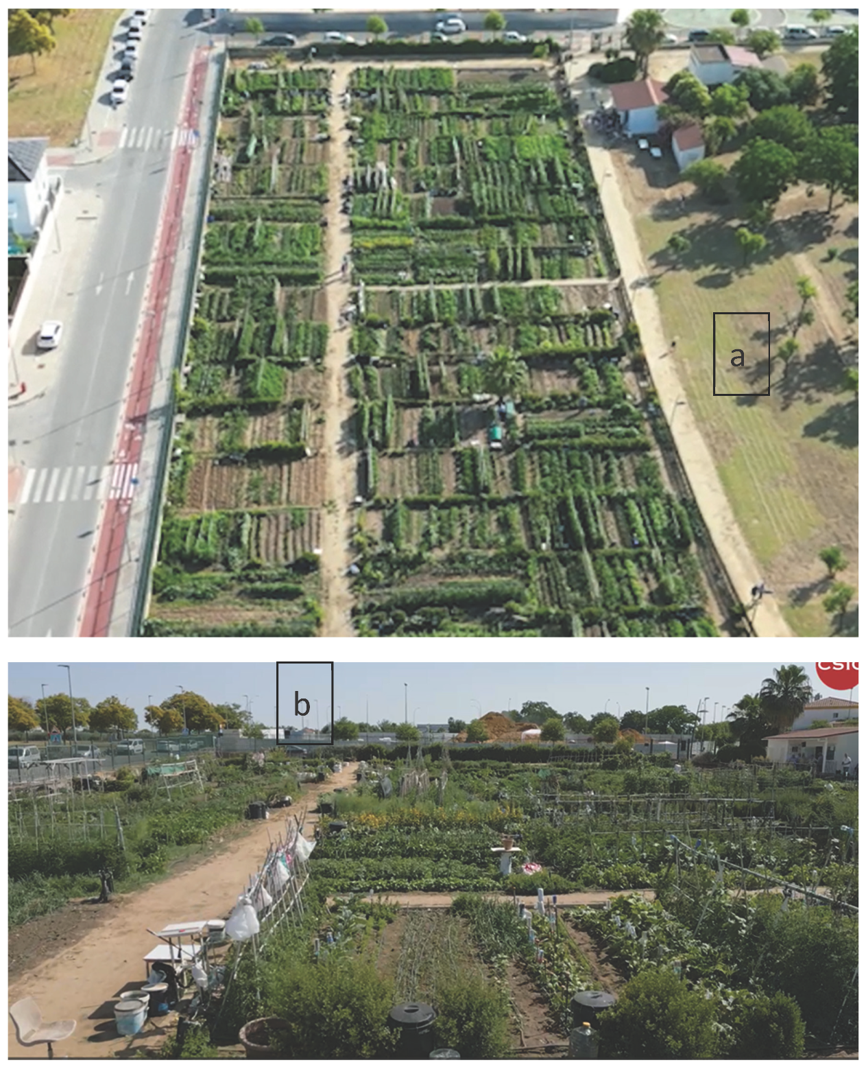
Figure 2.
Concentration factors and Pollution Load Index in both garden zones and in the Control soil.
Figure 2.
Concentration factors and Pollution Load Index in both garden zones and in the Control soil.
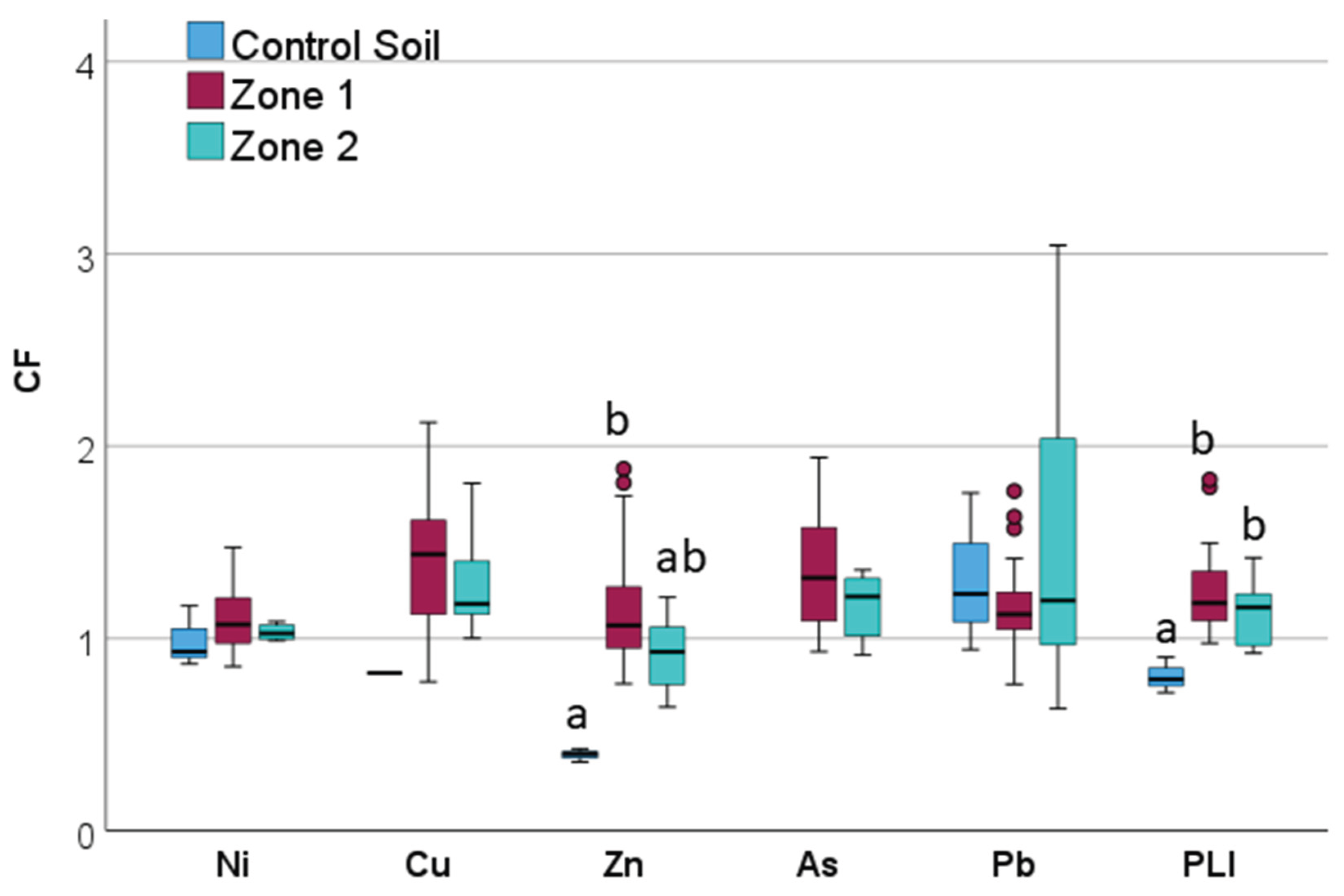
Figure 3.
Principal component analysis of soil properties in plots.
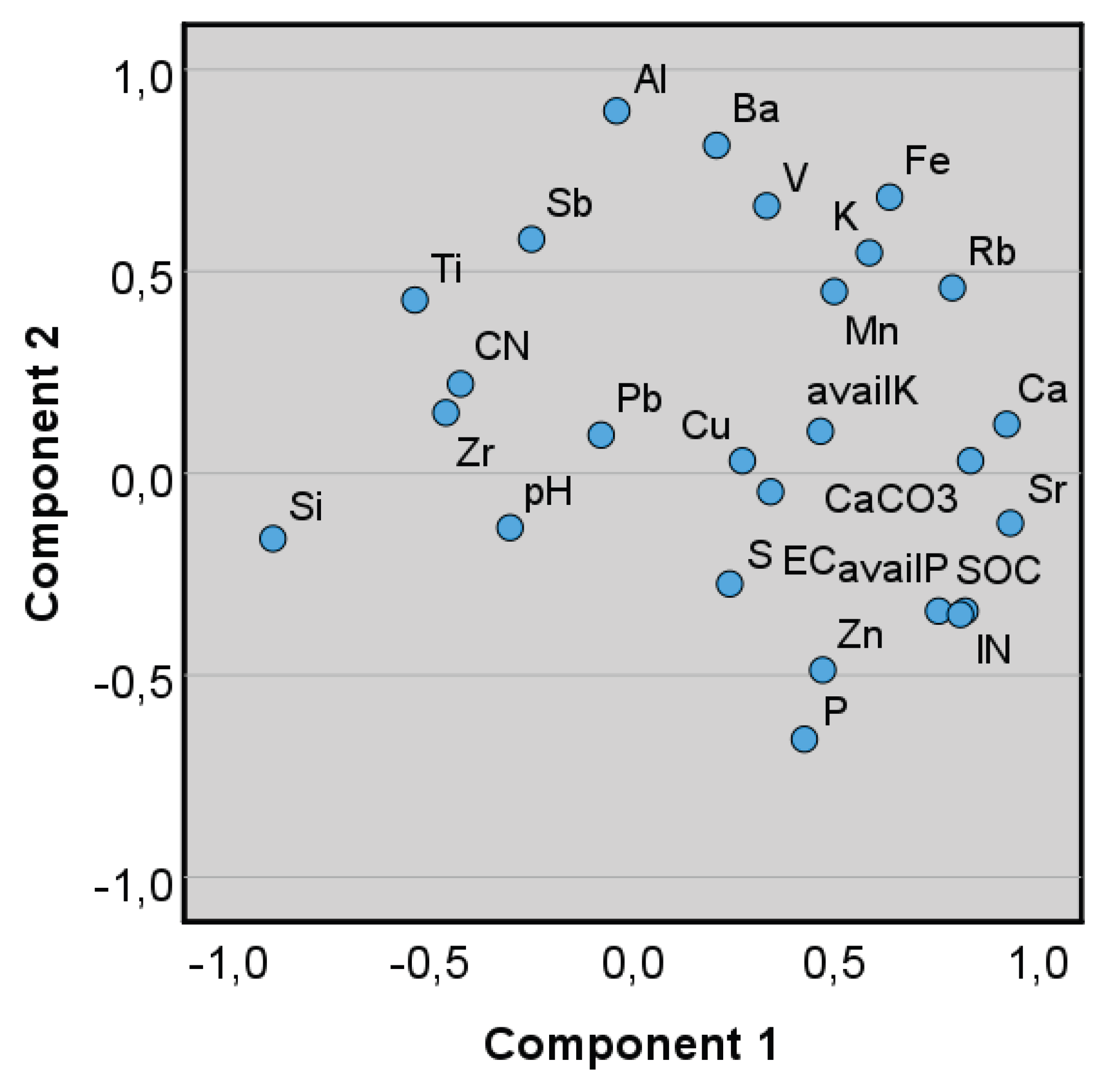
Figure 4.
Predicted values of available-K and available-P by the best linear fits versus the measured results.
Figure 4.
Predicted values of available-K and available-P by the best linear fits versus the measured results.
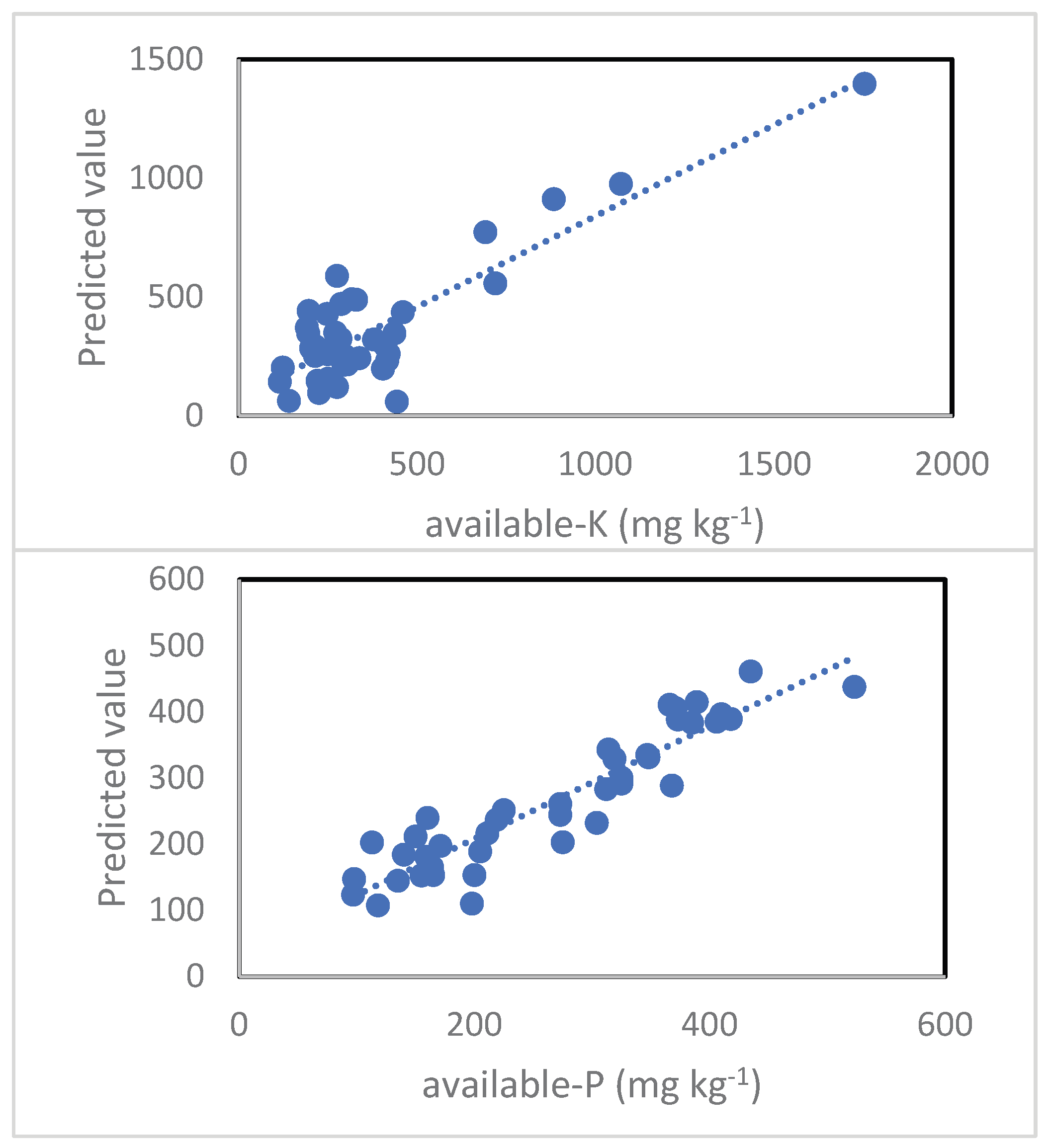
Figure 5.
Relationship between soil carbonate content and soil organic carbon (SOC).
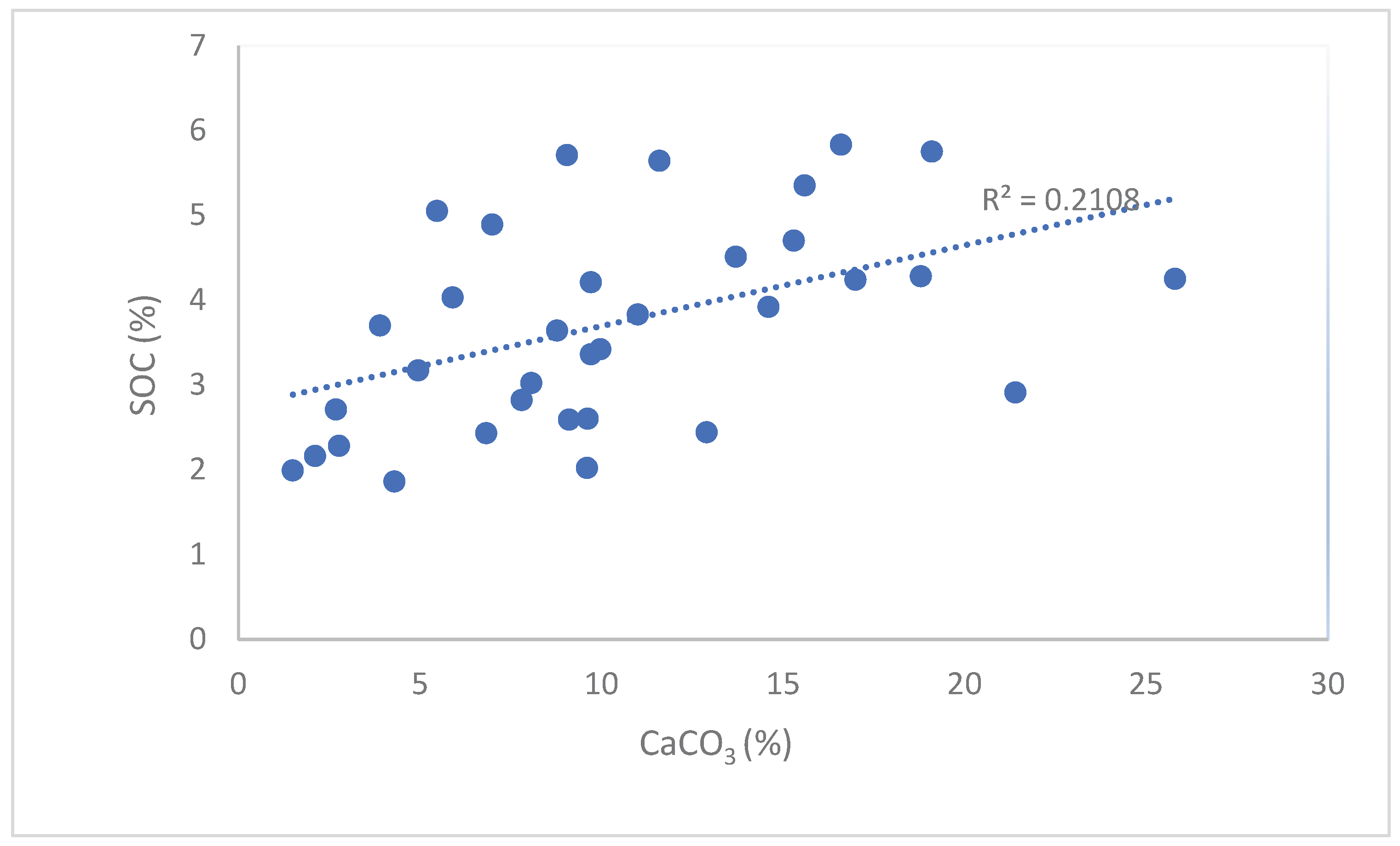

Table 1.
Performance of the instrument: Variations in daily measurements (N=7) of the certified reference material sediment SdAR-M2.
Table 1.
Performance of the instrument: Variations in daily measurements (N=7) of the certified reference material sediment SdAR-M2.
| Certified Value mg kg-1 |
Average value mg kg-1 |
Standard Deviation |
CV % |
Recovery % |
Minimum recovery % |
Maximum recovery % |
|
|---|---|---|---|---|---|---|---|
| Ag | 15 | 19.1 | 2.3 | 12.0 | 127.2 | 105.9 | 148.2 |
| As | 76 | 79.7 | 9.3 | 11.7 | 104.9 | 86.1 | 117.1 |
| Ba | 990 | 871 | 13.7 | 1.6 | 88.0 | 86.1 | 90.2 |
| Cr | 49.6 | 61.1 | 12.2 | 19.9 | 123.2 | 84.6 | 149.6 |
| Cu | 236 | 219 | 13.3 | 6.1 | 92.9 | 86.3 | 99.7 |
| Mn | 1038 | 844 | 28.8 | 3.4 | 81.3 | 76.0 | 84.8 |
| Ni | 48.8 | 76.4 | 6.1 | 8.0 | 156.6 | 134.7 | 177.2 |
| Pb | 808 | 796 | 17.9 | 2.2 | 98.5 | 93.6 | 99.9 |
| Rb | 149 | 133 | 3.2 | 2.4 | 89.5 | 85.5 | 91.6 |
| S | 970 | 1068 | 98.9 | 9.3 | 110.1 | 94.0 | 121.1 |
| Sb | 107 | 103 | 3.2 | 3.1 | 95.9 | 91.8 | 100.1 |
| Sr | 144 | 142 | 3.1 | 2.2 | 98.5 | 95.1 | 101.4 |
| Th | 14.2 | 16.9 | 3.1 | 18.1 | 119.0 | 87.5 | 145.7 |
| Ti | 1798 | 1407 | 97.1 | 6.9 | 78.3 | 67.2 | 83.1 |
| Zn | 760 | 716 | 17.5 | 2.4 | 94.2 | 90.6 | 98.2 |
| K × 10-3 | 41.5 | 37.6 | 2.5 | 6.8 | 90.7 | 78.4 | 96.4 |
| 1Fe × 10-3 | 18.4 | 18.5 | 0.2 | 1.0 | 100.7 | 99.2 | 101.7 |
| 1Ca × 10-3 | 6.00 | 5.88 | 0.14 | 2.4 | 98.0 | 94.1 | 101.5 |
| 1Mg × 10-3 | 2.96 | 4.63 | 1.24 | 26.9 | 156.4 | 92.9 | 205.7 |
| 1Al × 10-3 | 66.0 | 37.5 | 2.43 | 6.5 | 56.8 | 53.5 | 63.3 |
| 1Si × 10-3 | 343 | 292 | 13.0 | 4.4 | 85.1 | 79.9 | 90.7 |
| 1P | 345 | 549 | 91 | 16.8 | 159.1 | 129.9 | 183.8 |
1For these elements measurements were done in the precalibrated Mining mode; For the rest of the elements, the measurements were made with the precalibrated Soil mode.
Table 2.
Statistics of elemental concentrations in urban garden soil samples and elemental concentrations in the Control soil ( the elements are arranged in decreasing order of CV).
Table 2.
Statistics of elemental concentrations in urban garden soil samples and elemental concentrations in the Control soil ( the elements are arranged in decreasing order of CV).
| Control soil mg kg-1 |
Average value mg kg-1 |
Standard Deviation mg kg-1 |
CV1 % |
Minimum mg kg-1 |
Maximum mg kg-1 |
N2 | |
|---|---|---|---|---|---|---|---|
| S | 396 | 1337 | 769 | 57.5 | 598 | 5146 | 46 |
| Zn | 22.0 | 66.2 | 31.1 | 47.0 | 36.0 | 244.3 | 46 |
| 3Ca × 10-3 | 14.3 | 62.7 | 23.6 | 37.6 | 20.1 | 123.4 | 46 |
| Pb | 22.3 | 20.8 | 6.9 | 33.4 | 10.8 | 51.8 | 46 |
| P | 1390 | 2485 | 689 | 27.7 | 1009 | 3961 | 46 |
| Sr | 20.7 | 60.0 | 16.3 | 27.2 | 29.0 | 90.2 | 46 |
| Cu | 19.7 | 33.2 | 8.4 | 25.4 | 18.6 | 51.0 | 44 |
| Zr | 164 | 140 | 34.1 | 24.3 | 76.9 | 233 | 46 |
| As | bd | 7.85 | 1.74 | 22.2 | 5.48 | 11.64 | 25 |
| Ba | 215 | 202 | 43.6 | 21.5 | 104 | 291 | 46 |
| 3Fe × 10-3 | 10.7 | 12.6 | 2.4 | 18.7 | 8.85 | 19.4 | 46 |
| Sb | 23.2 | 18.6 | 3.4 | 18.5 | 12.7 | 26.4 | 38 |
| V | 35.7 | 37.6 | 6.9 | 18.3 | 28.7 | 57.2 | 44 |
| Mn | 166 | 169 | 29.1 | 17.2 | 110 | 257 | 46 |
| 3Al × 10-3 | 19.1 | 15.3 | 2.55 | 16.6 | 10.9 | 21.3 | 46 |
| Ni | 29.7 | 32.8 | 4.9 | 15.0 | 25.6 | 44.2 | 27 |
| 3Mg × 10-3 | bd | 5.13 | 0.76 | 14.7 | 4.47 | 6.30 | 5 |
| Rb | 19.3 | 23.9 | 3.5 | 14.6 | 18.0 | 31.1 | 46 |
| 3K × 10-3 | 7.01 | 7.48 | 1.09 | 14.5 | 5.42 | 10.9 | 46 |
| Ti | 2020 | 1607 | 227 | 14.2 | 1198 | 2172 | 46 |
| 3Si × 10-3 | 245.5 | 208.7 | 24.6 | 11.8 | 157.0 | 274.4 | 46 |
1Coefficient of variation; 2Number of cases above limit of detection; 3For these elements measurements were done in the precalibrated Mining mode, for the rest of the elements, the measurements were made with the precalibrated Soil method.
Table 3.
Fertility soil properties in urban garden and Control soil samples.
| Control soil mg kg-1 |
Average value mg kg-1 |
Standard Deviation mg kg-1 |
CV1 % |
Minimum mg kg-1 |
Maximum mg kg-1 |
N2 | ||
|---|---|---|---|---|---|---|---|---|
| Sector 1 and 2 | ||||||||
| pH | 7.36 | 7.41 | 0.40 | 5.50 | 6.33 | 8.21 | 41 | |
| EC3 | dS m-1 | 0.05 | 0.59 | 0.49 | 83.0 | 0.12 | 2.60 | 41 |
| CaCO3 | % | 1.93 | 9.86 | 5.48 | 55.6 | 1.50 | 25.80 | 41 |
| SOC4 | % | 1.23 | 3.57 | 1.18 | 33.2 | 1.86 | 5.83 | 41 |
| total-N | % | 0.073 | 0.355 | 0.116 | 32.7 | 0.203 | 0.605 | 41 |
| C/N | 16.6 | 10.1 | 1.2 | 12.2 | 8.3 | 13.2 | 41 | |
| avail-P5 | mg kg-1 | 26 | 264 | 108 | 41.0 | 97 | 523 | 46 |
| avail-K6 | mg kg-1 | 113 | 375 | 294 | 78.4 | 116 | 1755 | 41 |
| Sector 1 | ||||||||
| pH | 7.36 | 7.39 | 0.44 | 5.9 | 6.33 | 8.21 | 33 | |
| EC | dS m-1 | 0.05 | 0.57 | 0.39 | 67.7 | 0.12 | 1.67 | 33 |
| CaCO3 | % | 1.93 | *10.64 | 5.8 | 54.3 | 1.5 | 25.8 | 33 |
| SOC | % | 1.23 | *3.78* | 1.20 | 31.7 | 1.99 | 5.83 | 33 |
| total-N | % | 0.073 | *0.377* | 0.118 | 31.3 | 0.203 | 0.605 | 33 |
| C/N | 16.6 | *10.1 | 1.18 | 11.7 | 8.3 | 13.2 | 33 | |
| avail-P | mg kg-1 | 26 | *276 | 110 | 40.0 | 97 | 523 | 38 |
| avail-K | mg kg-1 | 113 | 412 | 315 | 76.4 | 142 | 1755 | 33 |
| Sector 2 | ||||||||
| pH | 7.36 | 7.49 | 0.23 | 3.1 | 7.22 | 7.84 | 8 | |
| EC | dS m-1 | 0.05 | 0.66 | 0.82 | 125 | 0.16 | 2.60 | 8 |
| CaCO3 | % | 1.93 | 6.64 | 2.09 | 31.5 | 3.9 | 9.5 | 8 |
| SOC | % | 1.23 | 2.72* | 0.66 | 24.3 | 1.86 | 3.70 | 8 |
| total-N | % | 0.073 | *0.264* | 0.045 | 17.1 | 0.208 | 0.344 | 8 |
| C/N | 16.6 | *10.2 | 1.52 | 14.9 | 8.6 | 12.4 | 8 | |
| avail-P | mg kg-1 | 26 | *208 | 83 | 39.8 | 113 | 370 | 8 |
| avail-K | mg kg-1 | 113 | 221 | 81 | 36.7 | 116 | 339 | 8 |
Table 4.
General properties and extractable aqua regia contents of manures and compost.
| Horse manure | Horse manure | Horse manure | Cow dung | Commercial compost | Biowaste compost |
||
| Moisture | % | 53.0 | 26.0 | 72.0 | 20.9 | 23.5 | 11.7 |
| pH | 8.85 | 7.88 | 8.14 | 7.58 | 9.05 | 8.51 | |
| E.C.1 | dS m-1 | 1.40 | 1.84 | 1.86 | 4.08 | 1.52 | 3.45 |
| Inorg-C | g kg-1 | 2.25 | 4.48 | 2.29 | 5.94 | 5.95 | 15.0 |
| Org-C | g kg-1 | 404 | 99.6 | 365 | 356 | 121 | 328 |
| OM2 | g kg-1 | 768 | 189 | 693 | 676 | 229 | 607 |
| N | g kg-1 | 13.9 | 9.34 | 14.0 | 22.5 | 12.9 | 32.6 |
| C/N ratio | 29.1 | 10.7 | 26.0 | 15.8 | 9.0 | 10.1 | |
| Ca | g kg-1 | 19.1 | 24.3 | 12.6 | 23.8 | 19.4 | 83.2 |
| K | g kg-1 | 12.0 | 5.68 | 19.4 | 15.1 | 11.3 | 11.4 |
| Mg | g kg-1 | 2.83 | 2.33 | 3.66 | 4.42 | 6.69 | 7.79 |
| Na | g kg-1 | 7.62 | 1.70 | 4.26 | 6.58 | 3.14 | 6.43 |
| S | g kg-1 | 2.66 | 1.55 | 2.53 | 3.90 | 2.55 | 5.52 |
| P | g kg-1 | 3.95 | 2.74 | 3.78 | 4.70 | 5.20 | 6.99 |
| Al | g kg-1 | 1.55 | 7.19 | 2.96 | 2.22 | 8.57 | 5.07 |
| As | mg kg-1 | < 1.0 | < 1.0 | < 1.0 | < 1.0 | 21.9 | 1.02 |
| B | mg kg-1 | 11.9 | 10.7 | 12.2 | 13.8 | 20.7 | 34.4 |
| Ba | mg kg-1 | 39.8 | 53.0 | 69.0 | 34.4 | 67.0 | 49.9 |
| Cd | mg kg-1 | 0.24 | 0.32 | 0.30 | 0.16 | 0.23 | 0.19 |
| Co | mg kg-1 | 0.55 | 2.39 | 0.87 | 1.44 | 3.80 | 1.31 |
| Cr | mg kg-1 | 10.1 | 38.2 | 10.9 | 12.9 | 92.8 | 40.2 |
| Cu | mg kg-1 | 10.8 | 23.6 | 8.1 | 22.1 | 46.6 | 56.7 |
| Fe | mg kg-1 | 1697 | 8286 | 2687 | 2546 | 9297 | 7097 |
| Li | mg kg-1 | 2.01 | 7.70 | 4.09 | 3.31 | 28.3 | 4.57 |
| Mn | mg kg-1 | 95.0 | 123 | 90.0 | 159 | 343 | 207 |
| Mo | mg kg-1 | 1.43 | 0.79 | 2.38 | 1.87 | 2.80 | 3.44 |
| Ni | mg kg-1 | 5.70 | 8.66 | 5.39 | 7.30 | 44.7 | 26.1 |
| Pb | mg kg-1 | 8.0 | 9.5 | 14.5 | 1.9 | 14.9 | 24.1 |
| Sn | mg kg-1 | 0.91 | 0.84 | 0.58 | 0.48 | 1.9 | 13.8 |
| Sr | mg kg-1 | 48.0 | 58.6 | 101.4 | 56.6 | 84.8 | 193 |
| V | mg kg-1 | 4.2 | 14.6 | 6.3 | 5.0 | 16.3 | 10.9 |
| Zn | mg kg-1 | 41.1 | 68.5 | 49.6 | 155.1 | 153.5 | 167 |
1E.C.: Electrical conductivity 1:5 vol/vol extract; 1OM: Organic matter content.
Table 5.
Results of multiple linear regression for the prediction of available-K and available-P.
| Predictor | t | Sig. | Importance |
|---|---|---|---|
| Available-K Accuracy 73.7% | |||
| K | 2.391 | 0.000 | 0.656 |
| Al | -4.275 | 0.000 | 0.133 |
| Mn | -3.097 | 0.004 | 0.070 |
| Zn | -2.896 | 0.007 | 0.061 |
| pH | -2.857 | 0.007 | 0.059 |
| Available-P Accuracy 83.6% | |||
| Sr | 7.403 | 0.000 | 0.436 |
| P | 6.218 | 0.000 | 0.307 |
| Al | 4.001 | 0.000 | 0.127 |
| Rb | -2.554 | 0.015 | 0.052 |
| Mn | -2.397 | 0.021 | 0.046 |
Table 6.
Coefficient of variation (%) of soil properties in selected plots (number in brackets indicates the number of cases).
Table 6.
Coefficient of variation (%) of soil properties in selected plots (number in brackets indicates the number of cases).
| Plot | 35 | 34 | 45 | Zone 1 |
|---|---|---|---|---|
| EC | 56.3 (6) | 16.5 (3) | 57.3 (4) | 67.7 (33) |
| CaCO3 | 21.0 (6) | 32.3 (3) | 15.0 (4) | 54.3 (33) |
| SOC | 14.2 (6) | 16.0 (3) | 32.6 (4) | 31.7 (33) |
| Total-N | 12.8 (6) | 9.1 (3) | 27.3 (4) | 31.3 (33) |
| avail-P | 7.7 (6) | 8.9 (4) | 14.3 (4) | 40.0 (38) |
| avail-K | 55.1 (6) | 34.5 (3) | 40.6 (4) | 76.4 (33) |
| S | 11.3 (6) | 6.9 (4) | 6.4 (4) | 40.8 (38) |
| Zn | 12.1 (6) | 6.4 (4) | 5.5 (4) | 47.8 (38) |
| Ca | 10.3 (6) | 5.8 (4) | 7.3 (4) | 37.1 (38) |
| Pb | 9.1 (6) | 18 (4) | 18.0 (4) | 17.2 (38) |
| Cu | 26.1 (6) | 7.6 (4) | 2.1 (4) | 26.0 (37) |
| Ni | 24.0 (4) | 7.8 (3) | -- | 15.9 (23) |
Disclaimer/Publisher’s Note: The statements, opinions and data contained in all publications are solely those of the individual author(s) and contributor(s) and not of MDPI and/or the editor(s). MDPI and/or the editor(s) disclaim responsibility for any injury to people or property resulting from any ideas, methods, instructions or products referred to in the content. |
© 2025 by the authors. Licensee MDPI, Basel, Switzerland. This article is an open access article distributed under the terms and conditions of the Creative Commons Attribution (CC BY) license (http://creativecommons.org/licenses/by/4.0/).
Copyright: This open access article is published under a Creative Commons CC BY 4.0 license, which permit the free download, distribution, and reuse, provided that the author and preprint are cited in any reuse.


