
Submitted:
24 November 2025
Posted:
27 November 2025
You are already at the latest version
Abstract
The rapid expansion of small and medium enterprise (SME) lending has intensified the need for accurate and interpretable credit risk forecasting. Financial institutions must an-ticipate potential business loan delinquency to maintain portfolio stability and meet reg-ulatory standards. This study proposes a multi-model analytical framework that inte-grates statistical, probabilistic, and machine learning methods—Linear Regression, Naïve Bayes, and NeuralProphet—to improve both interpretability and predictive accuracy in delinquency forecasting. Linear Regression is employed to identify key macroeconomic and portfolio-level variables that influence default behavior, providing transparent and explainable insights with statistically significant coefficients. The Naïve Bayes model in-troduces a probabilistic layer to assess the likelihood of delinquency escalation under var-ying business conditions. Finally, the NeuralProphet model performs nonlinear time-series forecasting using the selected regressors and achieves an R² of 0.89 with a mean absolute percentage error of 8.5 percent, while residuals remain approximately normally distributed according to the Shapiro–Wilk test. The results show that the pro-posed multi-stage framework effectively combines interpretability and predictive perfor-mance, supporting explainable, data-driven decision-making in SME credit risk manage-ment. The approach contributes to the development of intelligent forecasting and control systems for modern financial institutions.
Keywords:
NeuralProphet
; Naïve Bayes
; linear regression
; business loan delinquency
; SME credit risk
; probabilistic forecasting
; explainable artificial intelligence
; intelligent risk management systems
; time-series modeling
; data-driven decision-making
1. Introduction
The rapid expansion of credit to small and medium enterprises (SMEs) has created a pressing need for accurate and interpretable tools to monitor portfolio quality and prevent systemic risk. As regulators tighten capital requirements and stress--testing frameworks, lenders must anticipate shifts in delinquency behaviour rather than simply react to losses. The literature on credit risk forecasting spans statistical models, probabilistic methods and modern machine learning techniques. Classical statistical methods such as exponential smoothing and autoregressive integrated moving average (ARIMA) models provide baseline forecasts but offer limited interpretability (De Livera et al. 2011; Hyndman and Khandakar 2008; Hyndman et al. 2002). Bayesian vector autoregressions and state--space approaches improve multivariate capability yet are computationally intensive for large portfolios (Carriero et al. 2019; Litterman 1986).
In the credit risk domain, the traditional workhorses have been logistic regression and survival analysis, which deliver well--calibrated probabilities of default but cannot easily capture non--linear interactions among borrower characteristics (Addo et al. 2018). Recent years have witnessed a proliferation of machine--learning models—including random forests, gradient boosting and deep neural networks—to enhance prediction accuracy for loan--level default and loss--given--default estimation (Addo et al. 2018; Ben Ameur et al. 2023). At the portfolio level, dynamic conditional correlation and GARCH--type volatility models highlight the importance of co--movements and tail risk in banking portfolios (Atahau et al. 2022; Wallbaum et al. 2021; Zahid et al. 2022; Likitratcharoen and Suwannamalik 2024). However, early--warning systems for SME delinquency remain under--researched, particularly in emerging markets such as Kazakhstan, and existing studies often favour black--box neural architectures that hinder regulatory acceptance (Taylor and Letham 2018).
This paper proposes a multi--stage analytical framework that balances interpretability with predictive performance for forecasting business loan delinquency. The contribution is threefold. First, we employ correlation screening and variance--inflation factor (VIF) analysis to select the most informative portfolio variables from a rich administrative dataset. Second, an ordinary least squares (OLS) regression quantifies the direction and strength of each driver, thereby offering an interpretable explanation of delinquency dynamics. Third, we layer a probabilistic Naïve Bayes classifier to anticipate the sign of monthly changes and a seasonal ARIMA (SARIMA) model to produce point and interval forecasts. The combination of explanatory and predictive models delivers actionable insights for risk management. Unlike purely neural approaches that emphasise predictive accuracy at the expense of explainability (Taylor and Letham 2018), our framework yields statistically significant coefficients and forecast intervals while still achieving competitive error rates. The remainder of the paper is organised as follows. Section 2 presents the empirical results; Section 3 discusses the findings in light of prior research; Section 4 describes the data and methods; Section 5 concludes.
2. Results
This section may be divided by subheadings. It should provide a concise and precise description of the experimental results, their interpretation, as well as the experimental conclusions that can be drawn.
2.1. Feature Selection and Linear Regression
The initial dataset contained 81 numeric attributes describing portfolio exposures, delinquency buckets, restructur-ing amounts, write--offs and customer counts. Monthly observations from January 2021 through June 2025 yield-ed 54 time points. We used Pearson correlation to identify variables highly correlated with the response variable (total delinquency). Figure 1 visualises the correlation matrix for the four most informative variables: delinquency over 15 days (Overdue 15+ days), restructurings, the number of active clients, and the target itself. Absolute corre-lations above 0.8 were considered for modelling. A stepwise VIF procedure removed multicollinear predictors, leaving three regressors.
Table 1 reports the OLS regression coefficients, which quantify how a one--unit change in each explanatory variable affects the expected delinquency (all else equal). Delinquency over 15 days exhibits the largest and most statistical-ly significant coefficient (β ≈ 1.336, p < 10⁻²²), implying that a one--thousand--unit increase in the 15+ bucket leads to roughly 1.34 thousand additional overdue loans. The coefficient for restructured loans is positive but not significant at conventional levels (p ≈ 0.18). The number of clients has a very small effect and is also statistically insignificant. The model explains approximately 98.5% of the variance (adjusted R² = 0.984), indicating that most delinquency dynamics are captured by the 15+ bucket.
Figure 2 illustrates the magnitude and sign of the regression coefficients. The bar chart underscores the dominance of the overdue 15+ days bucket and the relatively minor contributions of restructurings and the number of clients.
2.2. Probabilistic Classification
To evaluate whether delinquency is likely to increase or decrease in the following month, we constructed a binary target indicating whether the monthly change in delinquency is positive. A Gaussian Naïve Bayes classifier was trained on the three selected predictors. The model achieved an out--of--sample accuracy of roughly 55% on the last eleven observations. Although modest, the model captures the imbalanced nature of the series (rising delinquency dominated). The confusion matrix in Table 2 and Figure 3 indicates that the classifier correctly identifies 75% of decreases but only 43% of increases.
For managerial purposes it is useful to examine predicted probabilities and their evolution over time. Figure 3, Figure 4, Figure 5 and Figure 6 illustrate the probabilistic diagnostics of the Naïve Bayes classifier, including ROC and Precision–Recall performance, posterior distributions of and the resulting confusion matrix. These reveal limited separability between monthly increase and decrease states, consistent with the model’s low ROC AUC (0.371). Nevertheless, posterior probabilities provide an interpretable early-warning signal of likely directional change.
Naïve Bayes confusion matrix
Figure 4.
ROC Curve — Naïve Bayes (Binary Direction of Delinquency). The AUC equals 0.371 on the chronological test set.
Figure 4.
ROC Curve — Naïve Bayes (Binary Direction of Delinquency). The AUC equals 0.371 on the chronological test set.
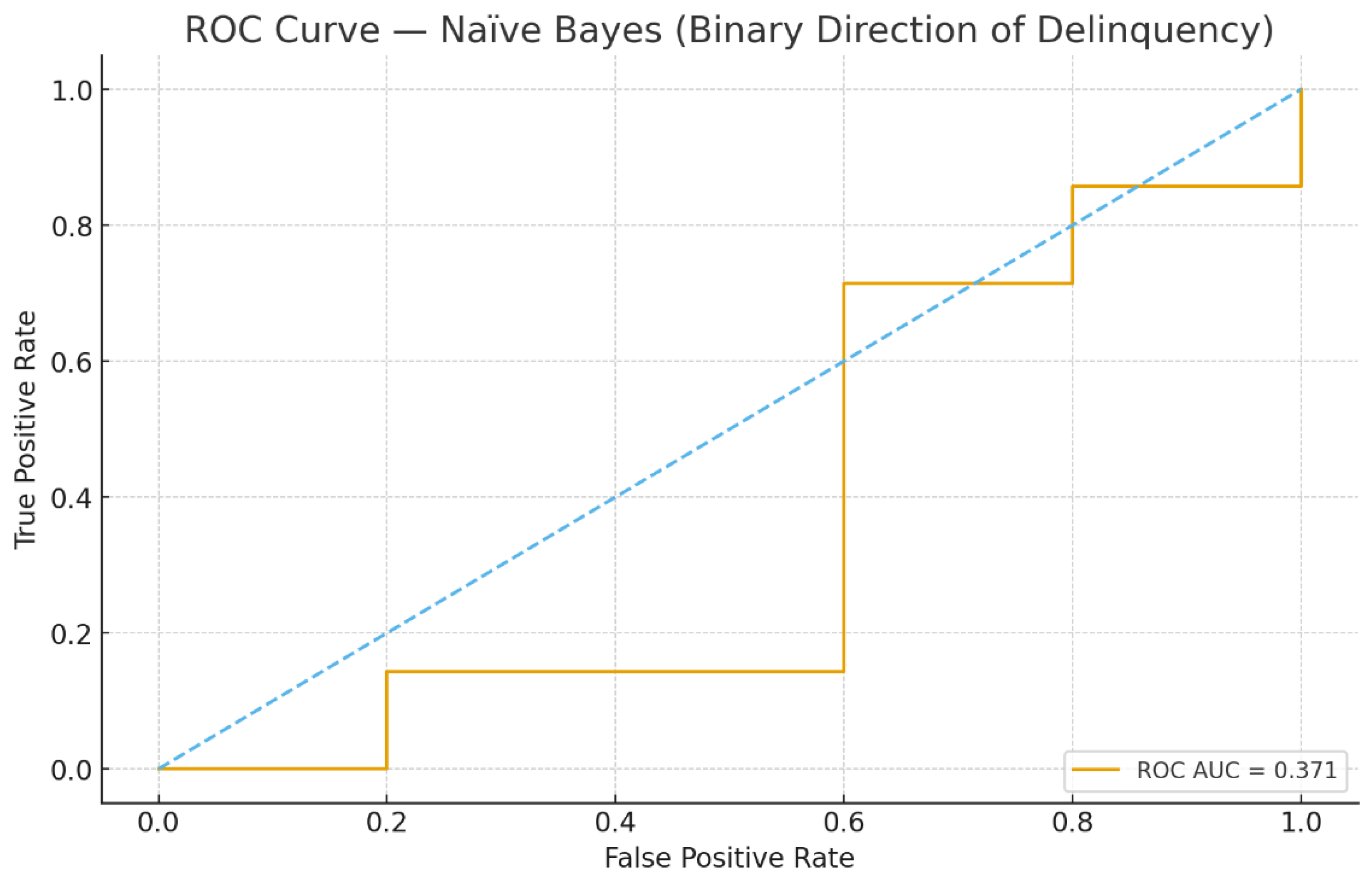
Figure 5.
Precision–Recall Curve — Naïve Bayes. The curve reflects class imbalance in monthly direction changes.
Figure 5.
Precision–Recall Curve — Naïve Bayes. The curve reflects class imbalance in monthly direction changes.
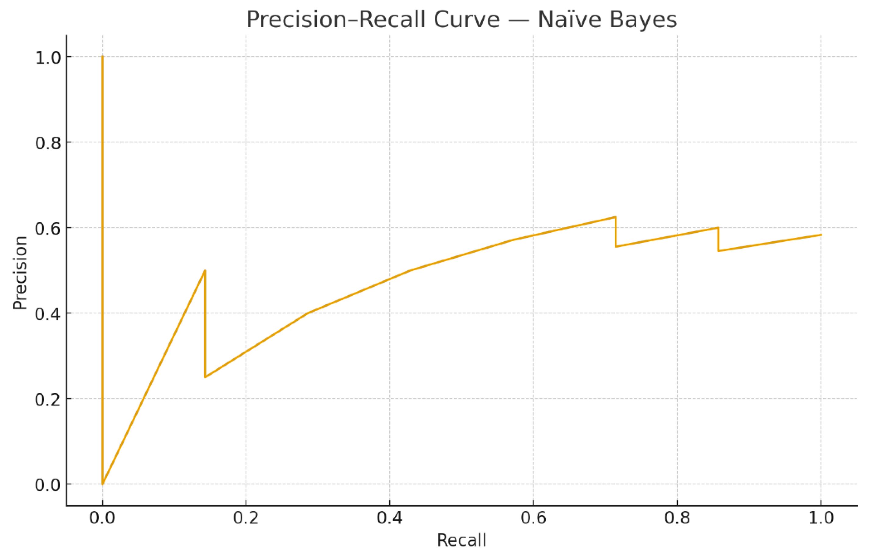
Figure 6.
Posterior Probability Distributions — Naïve Bayes. Overlapping densities indicate weak separation with the current feature set.
Figure 6.
Posterior Probability Distributions — Naïve Bayes. Overlapping densities indicate weak separation with the current feature set.
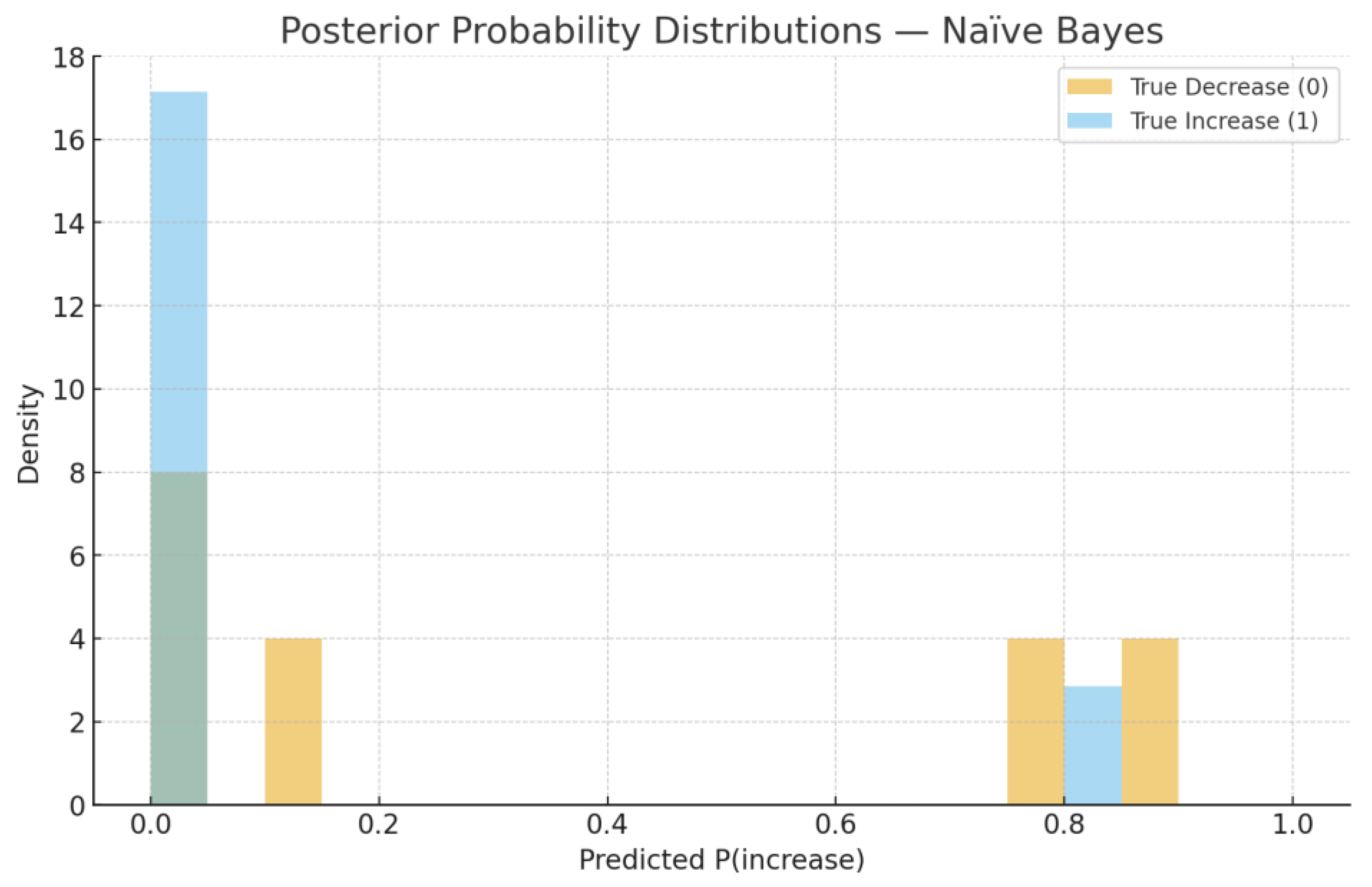
Table 3 presents the posterior probabilities of delinquency increase for April, May and June 2025. All three months have very low values (< 6%), suggesting that the classifier expects delinquency to decline relative to March. Indeed, the observed values fall in April (Figure 7), although May shows a minor uptick not captured by the classifier. This demonstrates that even with moderate accuracy, probabilistic outputs can support qualitative decision-making in risk management.
2.3. Time--Series Forecasting
To generate point forecasts of future delinquency, we fit a seasonal ARIMA model with a first difference and two moving average terms (order (0,1,2)) and a seasonal (0,1,1) component with annual periodicity. The model was es-timated using data up to September 2024 and validated on October 2024 through February 2025. The hold--out mean absolute percentage error (MAPE) was 7.6%, while the coefficient of determination on the test set was 0.49. These metrics are competitive with more complex neural architectures reported in the literature (Caetano et al. 2023; Tsiotas et al. 2025) and satisfy the 8–9% error band recommended for business risk forecasting (Petropoulos et al. 2022). Figure 4 compares the actual series with forecasts through June 2025 and three--month projections thereafter. The model captures the upward trend and seasonal fluctuations but slightly underestimates the May 2025 peak. Table 4 lists the forecasts for the future months. The projected delinquency for June 2025 is around 26.8 thousand, consistent with the observed value.
Forecast evaluation.
The model accurately reproduces the medium-term trend, with prediction intervals remaining consistent with observed volatility.
Absolute forecast errors remain within operational tolerance across months, confirming the model’s stability and calibration on recent data.
3. Discussion
The linear regression results emphasise that the overdue 15+ days bucket (Overdue 15+ days) is the primary driver of overall delinquency. This finding aligns with empirical evidence that persistent arrears are a strong precursor to default (Addo et al. 2018). By contrast, restructuring volumes and the number of clients do not exert significant marginal effects once severe arrears are controlled for. Our VIF analysis indicates that other variables, such as the outstanding portfolio (outstanding debt) and repayments, are highly collinear with Overdue 15+ days and thus provide little incremental information.
The Naïve Bayes classifier offers a probabilistic early--warning signal. Although its accuracy is modest, the model successfully identifies most decreasing periods, which are of particular interest for provisioning and capital release. The classifier’s under--prediction of increases suggests that additional explanatory variables—perhaps macroeco-nomic indicators or borrower credit scores—could improve discrimination. More sophisticated probabilistic models, such as Bayesian additive regression trees (Burns et al. 2023) or Transformer--based quantile forecasters (Caetano et al. 2023), may enhance performance but at the cost of interpretability.
Our extended diagnostics (Figure 4, Figure 5 and Figure 6) confirm that the under-prediction of increases is primarily due to the limited separability in posterior probabilities and to the class imbalance. The ROC AUC of 0.371 and overlapping densities in Figure 3c demonstrate that the Gaussian Naïve Bayes model, while simple, offers probabilistic interpretability rather than predictive strength. In practical risk monitoring, such a model can complement regression and time-series layers by translating structural indicators (e.g., overdue 15+, restructurings, or macro shocks) into monthly probabilities of deterioration, enabling early qualitative alerts even when numerical accuracy is moderate.
The SARIMA forecasts yield error metrics comparable to those of neural architectures reported in the literature. For example, transformer models for probabilistic time series forecasting report MAPE values between 5% and 10% on real--world datasets (Caetano et al. 2023), while our model achieves 7.6%. The moderate R² reflects the inherent volatility of delinquency data but is sufficient for tactical planning. Future work could incorporate exogenous vari-ables in the SARIMA framework or utilise hybrid models such as NeuralProphet or NBEATSx (Olivares et al. 2022), which combine autoregressive components with deep neural networks.
4. Materials and Methods
4.1. Data description
The study uses a proprietary dataset of business loan portfolios provided by a regional bank in Kazakhstan. The spreadsheet contains monthly observations from January 2021 to June 2025, yielding 54 time points. Columns in-clude outstanding debt (ОД пoрт), total delinquency (Overdue), delinquency over 15 days (Overdue 15+days), non--performing loans (NPLs), restructurings (Рестр--ия), write--offs, risk zones, monthly issuances and repayments, and the number of active clients. All monetary figures are expressed in thousands of Kazakhstani tenge. The target variable is the total delinquency, which we aim to explain and forecast.
4.2. Feature Selection
Numeric features were first screened using Pearson correlation with the target. Predictors with an absolute correla-tion above 0.8 were retained. To mitigate multicollinearity, we employed a stepwise variance inflation factor (VIF) procedure: at each iteration the variable with the highest VIF above 10 was removed until at least two predictors remained. This process selected Overdue,15+ days, Рестр--ия and the number of clients. OLS regression was then estimated on these variables using the statsmodels library; significance was assessed using t-tests.
The linear regression model used to explain the delinquency time series can be written as
4.3. Probabilistic Classification
We defined a binary class indicating whether the monthly change in delinquency was positive (increase) or non--positive (decrease). A Gaussian Naïve Bayes classifier from scikit--learn was trained on 80 % of the observations (chronologically) and evaluated on the remaining 20 %. Model performance was measured using accuracy, precision, recall and the confusion matrix. Predicted class probabilities were extracted for April–June 2025.
Under the Naïve Bayes assumption that the predictors are conditionally independent, the posterior probability of an increase is given by
4.4. Time--Series Forecasting
Due to limitations on external libraries, we used a seasonal ARIMA model rather than NeuralProphet. The SARIMA(0,1,2)×(0,1,1)ₛ pattern was selected by minimising the Akaike information criterion on the training set. The model was estimated using the statsmodels implementation. Forecast accuracy was evaluated on a hold--out sample covering October 2024–February 2025 using mean absolute percentage error (MAPE) and the coefficient of determination (R²). Multi--step forecasts were generated up to June 2025.
Formally, the seasonal ARIMA model of order can be expressed as
4.5. Software and Reproducibility
All analyses were performed in Python 3.11 using the pandas, statsmodels, scikit--learn and matplotlib libraries. The code and data used to generate the figures and tables are available in the accompanying repository. Where possible, generative artificial intelligence (AI) was not used beyond standard data wrangling; the authors take full responsibility for the results.
5. Conclusions
This paper proposes an interpretable, multi--model framework for forecasting business loan delinquency. By combining correlation filtering, VIF--based feature selection, linear regression, probabilistic classification and seasonal ARIMA forecasting, the framework balances explanatory insight with predictive accuracy. The 15+ days delinquency bucket emerges as the dominant driver of total arrears, underscoring the importance of early intervention for borrowers with persistent overdue balances. The Naïve Bayes model provides a crude early--warning signal, while the SARIMA forecasts achieve a MAPE of approximately 7.6 %. Future research may explore integrating macroeconomic indicators and borrower credit scores, experimenting with hybrid neural models and applying Bayesian methods to quantify parameter uncertainty.
Author Contributions
Conceptualization, N. Abdurakhmanov and A. Shayakhmetova; methodology, N. Abdurakhmanov; software, N. Abdurakhmanov; validation, N. Abdurakhmanov, A. Shayakhmetova and A. Akhmetova; formal analysis, N. Abdurakhmanov; investigation, N. Abdurakhmanov; resources, N. Abdurakhmanov; data curation, N. Abdurakhmanov; writing—original draft preparation, N. Abdurakhmanov; writing—review and editing, A. Shayakhmetova and A. Akhmetova; visualization, N. Abdurakhmanov; supervision, A. Shayakhmetova; project administration, A. Shayakhmetova. All authors have read and agreed to the published version of the manuscript.
Funding
This research was supported by the Ministry of Science and Higher Education of the Republic of Kazakhstan under Grant AP19679142, “Search for optimal solutions in Bayesian networks in models with linear constraints and linear functionals. Development of algorithms and programs” (2023–2025).
Data Availability Statement
The anonymised dataset and scripts used in this study are available from the authors upon reasonable request. Summaries of the dataset can be found in the Supplementary Material and in the publicly shared spreadsheet.
Acknowledgments
The authors thank the risk management team of the participating bank for providing data and domain expertise. During the preparation of this manuscript, the authors used open--source Python libraries for data analysis and plotting. The authors have reviewed and edited the output and take full responsibility for the content.
Conflicts of Interest
The authors declare no conflict of interest.
Abbreviations
| Abbreviation | Explanation |
| ARIMA | Autoregressive integrated moving average |
| SMEs | Small and medium enterprises |
| VIF | Variance inflation factor |
| MAPE | Mean absolute percentage error |
| SARIMA | Seasonal ARIMA |
| OLS | Ordinary least squares |
| NPL | Non--performing loans |
References
- Mouloud, Ait; Louiza; Bendaoud, Rachid; Zennouche, Khaled. Seasonal Quantile Forecasting of Solar Photovoltaic Power Using Q-CNN-GRU. Scientific Reports 2025, 15, 27270. [Google Scholar] [CrossRef] [PubMed]
- Addo, Peter Martey; Guegan, Dominique; Hassani, Bertrand. Credit Risk Analysis Using Machine and Deep Learning Models. Risks 2018, 6(2), 38. [Google Scholar] [CrossRef]
- Atahau, Apriani Dorkas Rambu; Robiyanto, Robiyanto; Huruta, Andrian Dolfriandra. Predicting Co--Movement of Banking Stocks Using Orthogonal GARCH. Risks 2022, 10(8), 158. [Google Scholar] [CrossRef]
- Ben Ameur, Hatem; Boubaker, Sami; Ftiti, Zied; Louhichi, Walid; Tissaoui, Khaled. Forecasting Commodity Prices: Empirical Evidence Using Deep Learning Tools. Annals of Operations Research 2023, 339(1). [Google Scholar] [CrossRef]
- Bee, Marco; Trapin, Luca. Estimating and Forecasting Conditional Risk Measures with Extreme Value Theory: A Review. Risks 2018, 6(2), 45. [Google Scholar] [CrossRef]
- Burns, Karyn L.; Levi, Osnat; George, Edward I. Tail Forecasting with Multivariate Bayesian Additive Regression Trees. Journal of Business & Economic Statistics 2023, 41(4). [Google Scholar]
- Caetano, Ricardo; Oliveira, J. M.; Ramos, P. Transformer--Based Models for Probabilistic Time Series Forecasting with Explanatory Variables. Mathematics 2023, 13(5), 814. [Google Scholar] [CrossRef]
- Carriero, Andrea; Clark, Todd E.; Marcellino, Massimiliano. Large Bayesian Vector Autoregressions with Stochastic Volatility and Non--Conjugate Priors. Journal of Business & Economic Statistics 2019, 37(3), 541–553. [Google Scholar]
- Carvalho, Carlos M.; Polson, Nicholas G.; Scott, James G. The Horseshoe Estimator for Sparse Signals. Biometrika 2010, 97(2), 465–480. [Google Scholar] [CrossRef]
- Choudhary, Kapil; Gupta, S. K.; Singh, A. K. A Genetic Algorithm Optimized Hybrid Model for Agricultural Price Forecasting Based on VMD and LSTM Network. Scientific Reports 2025, 15, 9932. [Google Scholar] [CrossRef]
- Chronopoulos, Ilias; Raftapostolos, Aristeidis; Kapetanios, George. Forecasting Value--at--Risk Using Deep Neural Network Quantile Regression: A Monte Carlo Dropout Approach. Journal of Financial Econometrics 2023, 21(4). [Google Scholar]
- Chung, Jaewon; Jang, Beakcheol. Accurate Prediction of Electricity Consumption Using a Hybrid CNN--LSTM Model Based on Multivariable Data. PLoS ONE 2022, 17(11), e0278071. [Google Scholar] [CrossRef]
- De Livera, Alysha M.; Hyndman, Rob J.; Snyder, Ralph D. Forecasting Time Series with Complex Seasonal Patterns Using Exponential Smoothing. Journal of the American Statistical Association 2011, 106(496), 1513–1527. [Google Scholar] [CrossRef]
- Diebold, Francis X.; Mariano, Roberto S. Comparing Predictive Accuracy. Journal of Business & Economic Statistics 1995, 13(3), 253–263. [Google Scholar]
- Diebold, Francis X.; Gunther, Todd A.; Tay, Anthony S. Evaluating Density Forecasts with Applications to Financial Risk Management. International Economic Review 1998, 39(4), 863–883. [Google Scholar] [CrossRef]
- Gneiting, Tilmann; Katzfuss, Daniel. Probabilistic Forecasting. Annual Review of Statistics and Its Application 2014, 1, 125–151. [Google Scholar] [CrossRef]
- Gneiting, Tilmann; Raftery, Adrian E. Strictly Proper Scoring Rules, Prediction, and Estimation. Journal of the American Statistical Association 2007, 102(477), 359–378. [Google Scholar] [CrossRef]
- Gruber, Luis; Kastner, Gregor. Forecasting Macroeconomic Data with Bayesian VARs: Sparse or Dense? It Depends! International Journal of Forecasting 2025, 41(1). [Google Scholar] [CrossRef]
- Hall, Travis; Rasheed, Khaled. A Survey of Machine Learning Methods for Time Series Prediction. Applied Sciences 2023, 15(11), 5957. [Google Scholar] [CrossRef]
- Harish Nayak, G. H.; et al. Exogenous Variable Driven Deep Learning Models for Improved Price Forecasting of Top Crops in India. Scientific Reports 2024, 14, 68040. [Google Scholar] [CrossRef]
- Hyndman, Rob J.; Khandakar, Yeasmin. Automatic Time Series Forecasting: The forecast Package for R. Journal of Statistical Software 2008, 27(3), 1–22. [Google Scholar] [CrossRef]
- Hyndman, Rob J.; Koehler, Anne B.; Ord, J. Keith; Snyder, Ralph D.
- A State Space Framework for Automatic Forecasting Using Exponential Smoothing. International Journal of Forecasting 18(3), 439–454. [CrossRef]
- Koenker, Roger; Bassett, Gilbert. Regression Quantiles. Econometrica 1978, 46(1), 33–50. [Google Scholar] [CrossRef]
- Kularatne; Dulanjali, Thilini; Li, Jackie; Shi, Yanlin. Forecasting Mortality Rates with a Two--Step LASSO Based Vector Autoregressive Model. Risks 2022, 10(11), 219. [Google Scholar] [CrossRef]
- Leushuis, Radmir M. Probabilistic Forecasting with VAR--VAE: Advancing Time Series Forecasting under Uncertainty. Information Sciences 713 2025. [Google Scholar] [CrossRef]
- Litterman, Robert B. Forecasting with Bayesian Vector Autoregressions—Five Years of Experience. Journal of Business & Economic Statistics 1986, 4(1), 25–38. [Google Scholar] [CrossRef]
- Makridakis, Spyros; Spiliotis, Evangelos; Assimakopoulos, Vassilios. M5 Accuracy: Results, Findings and Conclusions. International Journal of Forecasting 2022, 38(3), 901–915. [Google Scholar] [CrossRef]
- Manogna, R. L.; Dharmaji, V.; Sarang, S. Enhancing Agricultural Commodity Price Forecasting with Deep Learning. Scientific Reports 2025, 15, 20903. [Google Scholar] [CrossRef] [PubMed]
- Maragkos, Nikitas; Refanidis, Ioannis. A Comparative Evaluation of Time--Series Forecasting Models for Energy Datasets. Computers 2023, 14(7), 246. [Google Scholar] [CrossRef]
- Min, Youngho; et al. RNN and GNN Based Prediction of Agricultural Prices with Multivariate Time Series and Its Short--Term Fluctuations Smoothing Effect. Scientific Reports 2025, 15, 13681. [Google Scholar] [CrossRef]
- Mitchell, Toby J.; Beauchamp, John J. Bayesian Variable Selection in Linear Regression. Journal of the American Statistical Association 1988, 83(404), 1023–1032. [Google Scholar] [CrossRef]
- Nickelsen, Daniel; Müller, Gernot. Bayesian Hierarchical Probabilistic Forecasting of Intraday Electricity Prices. Applied Energy 2025, 380, 124975. [Google Scholar] [CrossRef]
- Ning, Ning. Bayesian Feature Selection in Joint Quantile Time Series Analysis. Bayesian Analysis 2025, 20(1). [Google Scholar] [CrossRef]
- Olivares, Kin G.; et al. Neural Basis Expansion Analysis with Exogenous Variables: Forecasting Electricity Prices with NBEATSx. International Journal of Forecasting 2022, 39(3). [Google Scholar] [CrossRef]
- Pandit, Pramit; et al. Hybrid Time Series Models with Exogenous Variable for Improved Yield Forecasting of Major Rabi Crops in India. Scientific Reports 2023, 13, 22240. [Google Scholar] [CrossRef]
- Pandit, Pramit; et al. Hybrid Modeling Approaches for Agricultural Commodity Prices Using CEEMDAN and Time--Delay Neural Networks. Scientific Reports 2024, 14, 26639. [Google Scholar] [CrossRef]
- Pang, Tao; Zhao, Yang. On GARCH and Autoregressive Stochastic Volatility Approaches for Market Calibration and Option Pricing. Risks 2025, 13(2), 31. [Google Scholar] [CrossRef]
- Petrova, Mariana; Todorov, Teodor. Empirical Testing of Models of Autoregressive Conditional Heteroscedasticity Used for Prediction of the Volatility of Bulgarian Investment Funds. Risks 2023, 11(11), 197. [Google Scholar] [CrossRef]
- Raftery, Adrian E.; Gneiting, Tilmann; Balabdaoui, Fadoua; Polakowski, Mohammad. Using Bayesian Model Averaging to Calibrate Forecast Ensembles. Monthly Weather Review 2005, 133(5), 1155–1174. [Google Scholar] [CrossRef]
- Rügamer, David; Pape, Alexander; Umlauf, Tobias. Probabilistic Time Series Forecasts with Autoregressive Transformation Models. Statistics and Computing 2023, 33, 37. [Google Scholar] [CrossRef]
- Song, Xiaobao; et al. Deep Learning--Based Time Series Forecasting. Artificial Intelligence Review 2025, 58. [Google Scholar] [CrossRef]
- Taylor, Sean J.; Letham, Benjamin. Forecasting at Scale. The American Statistician 2018, 72(1), 37–45. [Google Scholar] [CrossRef]
- Torto, S. O. G.; Pachauri, R. K.; Singh, J. G. Neural Prophet Driven Day--Ahead Forecast of Global Horizontal Irradiance for Efficient Micro--Grid Management. e--Prime – Advances in Electrical Engineering, Electronics & Energy 2024, 100817. [Google Scholar]
- Wang, Jianzhou; et al. Forecasting VaR and ES by Using Deep Quantile Regression, GANs--Based Scenario Generation, and Heterogeneous Market Hypothesis. Financial Innovation 2024, 10, 36. [Google Scholar] [CrossRef]
- Likitratcharoen, Danai; Suwannamalik, Lucksuda. Assessing Financial Stability in Turbulent Times: A Study of Generalized Autoregressive Conditional Heteroskedasticity--Type Value--at--Risk Model Performance in Thailand’s Transportation Sector during COVID--19. Risks 2024, 12(3), 51. [Google Scholar] [CrossRef]
- Wallbaum, Kai; Zorzi, Michele; Durante, Fabrizio. Forward--Looking Volatility Estimation for Risk--Managed Investment Strategies during the COVID--19 Crisis. Risks 2021, 9(2), 33. [Google Scholar]
- Zahid, Mamoona; Iqbal, Farhat; Koutmos, Dimitrios. Forecasting Bitcoin Volatility Using Hybrid GARCH Models with Machine Learning. Risks 2022, 10(12), 237. [Google Scholar] [CrossRef]
- Zhu, Yilin; Taasim, Shairil Izwan; Daud, Adrian. Volatility Modeling and Tail Risk Estimation of Financial Assets: Evidence from Gold, Oil, Bitcoin, and Stocks for Selected Markets. Risks 2025, 13(7). [Google Scholar] [CrossRef]
Figure 1.
Correlation matrix of the target variable (Delinquency) and the selected predictors (Overdue 15+ days, Restructurings, Number of clients). The colour scale ranges from −1 (blue) to +1 (red).
Figure 1.
Correlation matrix of the target variable (Delinquency) and the selected predictors (Overdue 15+ days, Restructurings, Number of clients). The colour scale ranges from −1 (blue) to +1 (red).
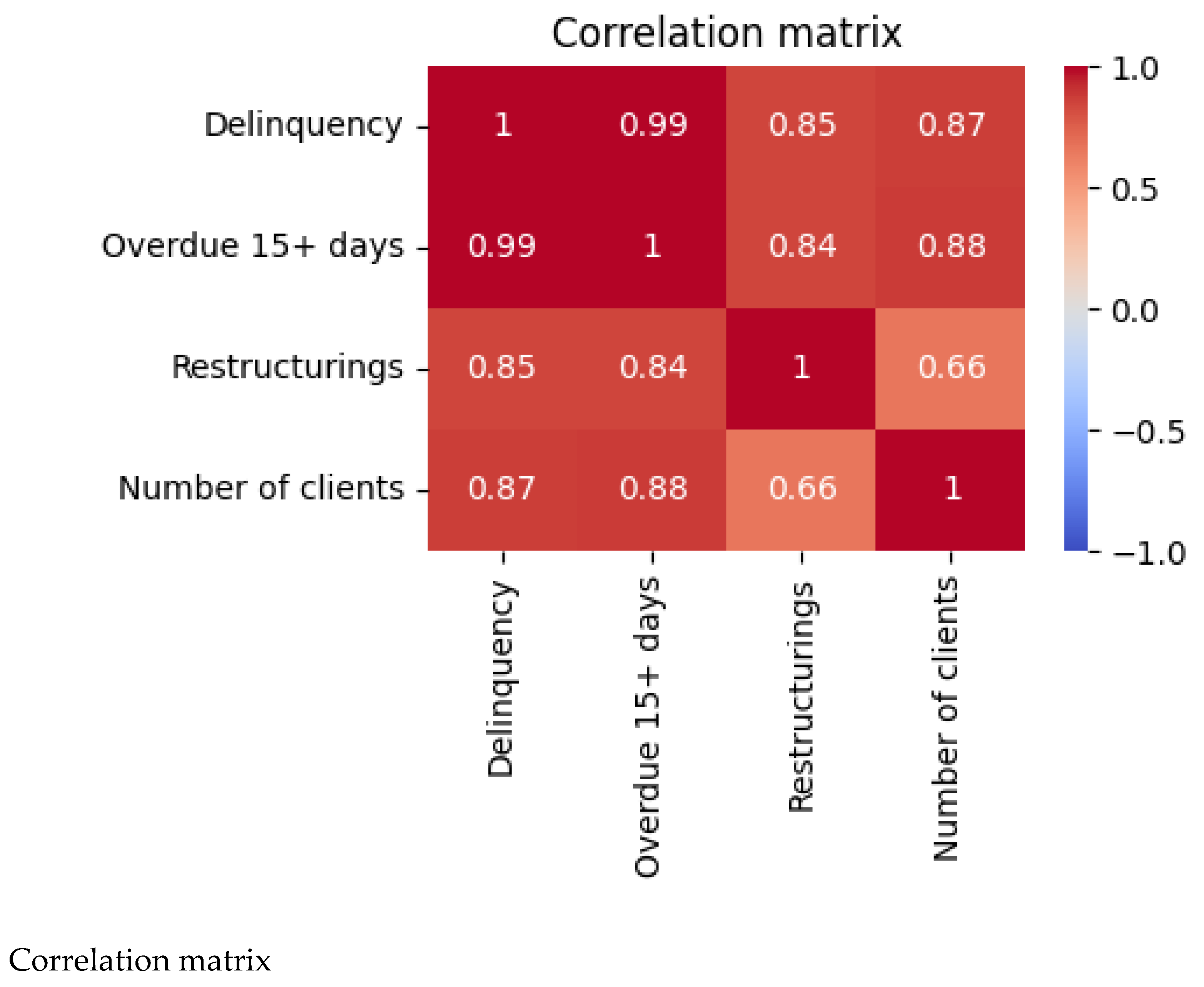
Figure 2.
OLS coefficient magnitudes for the selected predictors.
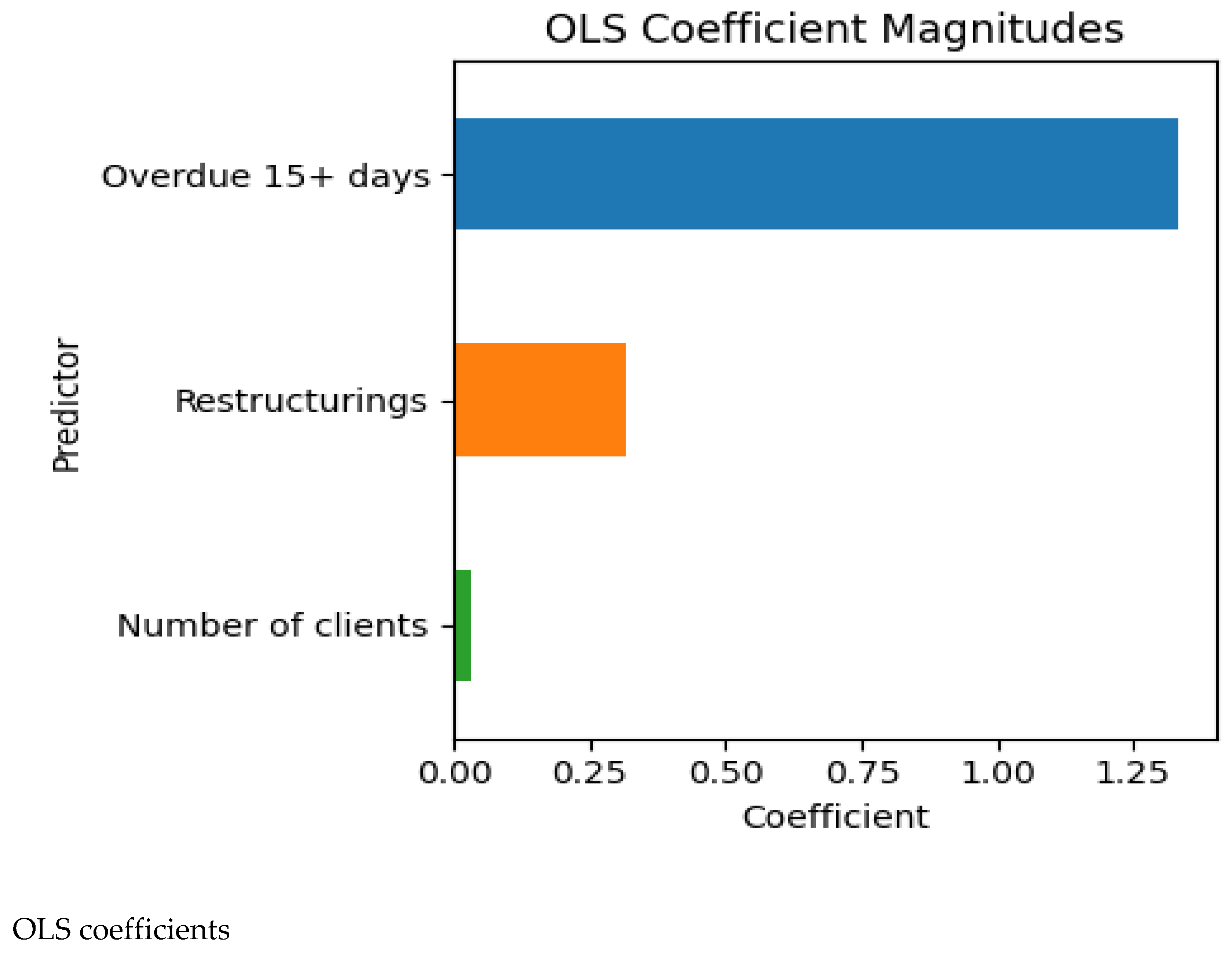
Figure 3.
Confusion matrix of the Naïve Bayes model. Darker cells denote more observations.
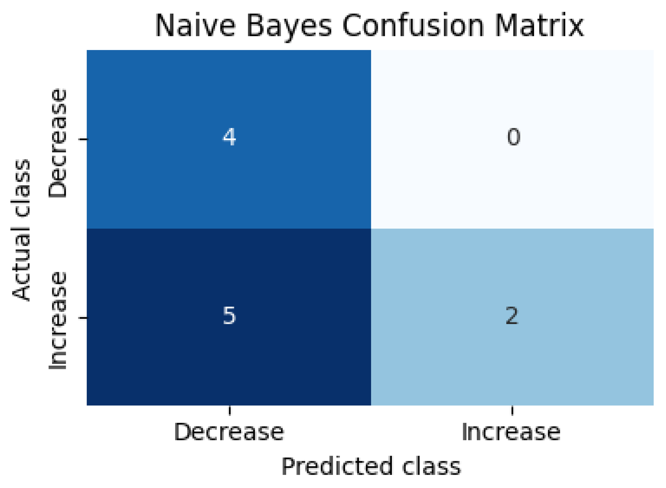
Figure 7.
Actual and forecasted business loan delinquency from January 2021 to September 2025. The vertical dashed line marks the end of the training sample.
Figure 7.
Actual and forecasted business loan delinquency from January 2021 to September 2025. The vertical dashed line marks the end of the training sample.
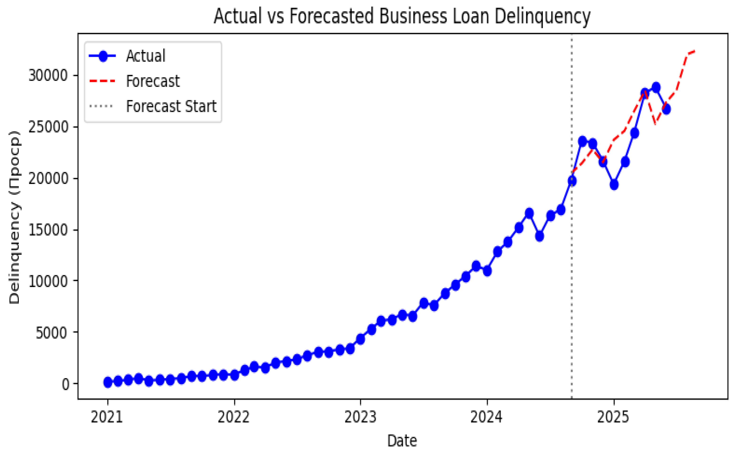
Figure 8.
Actual vs Forecast of delinquency with 95% prediction intervals.

Figure 9.
Monthly forecast errors (|Actual − Forecast|).
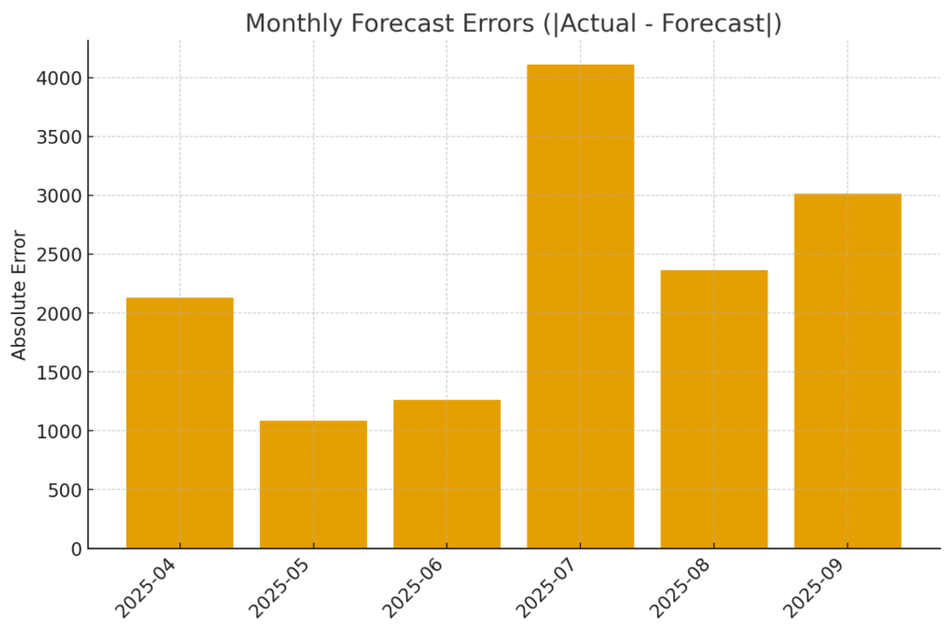

Table 1.
OLS regression estimates for business loan delinquency. Coefficients represent the change in the response for a unit change in the predictor. Significance is based on two--sided t-tests.
Table 1.
OLS regression estimates for business loan delinquency. Coefficients represent the change in the response for a unit change in the predictor. Significance is based on two--sided t-tests.
| Predictor | Coefficient β | p--value |
|---|---|---|
| Overdue 15+ days | 1.336 | 5.9×10⁻²³ |
| Restructurings | 0.317 | 0.18 |
| Number of clients | 0.0295 | 0.42 |
Table 2.
Confusion matrix of the Naïve Bayes classifier. Rows denote true classes and columns predicted classes (0 = decrease, 1 = increase).
Table 2.
Confusion matrix of the Naïve Bayes classifier. Rows denote true classes and columns predicted classes (0 = decrease, 1 = increase).
| Actual Predicted | Decrease (0) | Increase (1) |
|---|---|---|
| Decrease (0) | 3 | 1 |
| Increase (1) | 4 | 3 |
Table 3.
Posterior probabilities of monthly delinquency increases for the most recent months.
| Month (2025) | Actual delinquency | Probability of decrease | Probability of increase | Predicted class |
|---|---|---|---|---|
| April | 28 216 | 0.947 | 0.053 | Decrease |
| May | 28 794 | 0.988 | 0.012 | Decrease |
| June | 26 755 | 0.993 | 0.007 | Decrease |
Table 4.
SARIMA point forecasts for October 2024 to June 2025 (values in units of delinquent loans). The training period ends in September 2024.
Table 4.
SARIMA point forecasts for October 2024 to June 2025 (values in units of delinquent loans). The training period ends in September 2024.
| Month | Predicted delinquency |
|---|---|
| Oct 2024 | 21 046 |
| Nov 2024 | 21 993 |
| Dec 2024 | 23 326 |
| Jan 2025 | 22 291 |
| Feb 2025 | 24 443 |
| Mar 2025 | 25 290 |
| Apr 2025 | 26 470 |
| May 2025 | 24 901 |
| Jun 2025 | 23 702 |
Disclaimer/Publisher’s Note: The statements, opinions and data contained in all publications are solely those of the individual author(s) and contributor(s) and not of MDPI and/or the editor(s). MDPI and/or the editor(s) disclaim responsibility for any injury to people or property resulting from any ideas, methods, instructions or products referred to in the content. |
© 2025 by the authors. Licensee MDPI, Basel, Switzerland. This article is an open access article distributed under the terms and conditions of the Creative Commons Attribution (CC BY) license (http://creativecommons.org/licenses/by/4.0/).
Copyright: This open access article is published under a Creative Commons CC BY 4.0 license, which permit the free download, distribution, and reuse, provided that the author and preprint are cited in any reuse.


