
Submitted:
24 November 2025
Posted:
27 November 2025
You are already at the latest version
Abstract
Due to their complexity and non-linearity, metaheuristic algorithms have become the gold standard in problem solving for those problems that cannot be solved by standard computational solutions. However, the global performance of these algorithms is strongly linked to the population structuring and the mechanism of replacing the worst solutions within the population. In this paper, an Adaptive Artificial Hummingbird Algorithm (AAHA), a new version of the basic AHA, is introduced and designed to enhance performance by studying the impacts of different population initialization methods within a broad and continual migration form. For the initialization phase, four methods: the Gaussian chaotic map, the Sinus chaotic map, the Opposite-based learning (OBL), and the Diagonal Uniform Distribution (DUD) are proposed as an alternative to the random population initialization method. A new strategy is proposed for replacing the worst solution in the migration phase. The new strategy used the best solution as an alternative to the worst solution with simple and effective local search. The proposed strategy stimulates exploitation and exploration when using the best solution and local search, respectively. The proposed AAHA algorithm is tested through various benchmark functions with different characteristics under many statistical indices and tests. Additionally, the AAHA results are benchmarked against other optimization algorithms to assess their effectiveness. The proposed AAHA algorithm outperformed alternatives in both speed and reliability. DUD-based initialization enabled the fastest convergence and optimal solutions. These findings underscore the significance of initialization in metaheuristics and highlight the efficacy of the AAHA algorithm for complex continuous optimization problems.
Keywords:
artificial hummingbird algorithm
; diagonal uniform distribution
; opposition-based learning
; metaheuristic algorithms
; chaotic maps
; population initialization
1. Introduction
In the last few years, metaheuristic optimization algorithms were preferred because they can solve challenging, nonlinear optimization problems that traditional approaches can’t solve. These algorithms are useful in many areas, such as industrial design, process optimization, and intelligent electronics, because they can deal with many non-convex search spaces efficiently [1,2]. By imitating natural processes, metaheuristics help to find a balance between exploration and exploitation during the search process. For instance, Kennedy and Eberhart proposed the particle swarm optimization (PSO) algorithm in 1995 [1], which has become the most widely used example of a metaheuristic for solving real-world optimization problems Meanwhile, Dorigo and Stutzle [2] developed the ant colony optimization (ACO)algorithm, and Karaboga [3] came up with the artificial bee colony (ABC) algorithm. Storn and Price [4] also created the (DE) algorithm. Zhao et al. [5] have recently introduced the Artificial Hummingbird Algorithm (AHA), which is a novel optimization algorithm inspired by nature. Although these algorithms are effective, metaheuristic algorithms continue to face numerous critical challenges, including premature or delayed convergence, the identification of local optima, excess of solutions, and the inability to achieve an optimal balance between exploration and exploitation. The quality of the initial population has a big effect on how well the algorithms work. This affects their ability to explore the search space and stay away from local optima [6,7]. Recent research advances this subject further. Li et al. [8], for example, claim that starting with random values leads to a Gauss-like distribution of people, which means less diversity at first and worse performance. Advanced initialization strategies [7,8] such as Chaotic initialization, which relies on the specific behavior of chaotic coverage become effective alternative solutions. Opposition-Based Learning (OBL) increases the chances of finding solutions near optimal areas by creating the original and its counterpart and then evaluating the two sets of individuals simultaneously [6,9]. Moreover, other techniques were proposed such as Diagonal uniform distribution [7,10] to overcome the crowding and achieve uniform distribution in each dimension. Lastly, Dirichlet-based opposition, which avoids overcrowding and thus achieves successful OBL is another successful method in OBL [10]. Accordingly, new or nature-inspired algorithms with more intelligent and dynamic search mechanisms have been proposed to improve search efficiency [5,6].
The AHA algorithm effectively replicates the flight patterns and foraging behavior of hummingbirds, utilizing three primary feeding processes and three flight skills to maintain an active balance between exploration and exploitation. Despite that AHA effectively identify high-quality solutions, it is like most evolutionary algorithms, employs a fully random population initialization, which constrains individual variety in the early phases and impacts convergence speed. Moreover, the initial migration technique is constrained in its capacity to enhance search scalability in subsequent phases.
This paper provides a new version of AHA that is called the adaptive Artificial Hummingbird Algorithm (AAHA) and it is done by improving the initialization and migration phases of the algorithm. Four initialization approaches are evaluated for initializing the population which are Chaotic–Gauss, Chaotic–Sinus, Opposition Based Learning (OBL), and Diagonal Uniform Distribution (DUD) to ensure the diversity of initial solutions in the initial population. In conventional AHA, is assumed to be the worst solutions of the population that are replaced with other solutions that are randomly initiated in the migration phase. In the proposed adaptive AHA (AAHA) algorithm, the worst solutions are replaced with the best solution in order to increase exploitation by applying a simple local search to increase the exploration property. To ensure a fair comparison, all other elements of the method, including the migration operator, were kept unchanged across all configurations.
2. Related Work
The initialization and updating steps of individuals are crucial variables influencing the effectiveness of metaheuristic algorithms in achieving high-quality solutions. Many studies show that improving the initial distribution of individuals or developing new ways for them to move can greatly improve performance compared to standard random initialization or standard procedures [7,11]. This section analyses the primary research developments related to population initialization and migration methodologies.
2.1. Population Initialization in Metaheuristics
Recent research shows that the initialization phase is critical for any population-based algorithm, as the quality of individual distribution influences the initial diversity in the search space and the algorithm’s ability to avoid local optima [7,8,11]. Sarhani et al. [7] and Agushaka et al. [11] worked on different initialization methods by separating them into three groups namely chaotic-based, opposition-based, and uniform distribution-based. below is summary of the most important methods.
2.1.1. Chaotic Initialization (Gauss Map, Sinus Map)
Chaotic methods use nonlinear dynamic mathematical map functions that shuffle numbers to produce initial vectors with pseudo-random coverage characteristics. Unlike complete randomness, these methods retain more structure. The Gauss map and the Sinus map are two types of functions frequently used. They are effective in increasing variety within a population [8,12].
Kuang et al. [12] presented the Chaotic Artificial Bee Colony (CABC) algorithm, which combines chaotic maps—structured randomizing functions—with the artificial bee algorithm, thus improving the algorithm’s search efficiency for problems involving many peaks. Li et al. [8] claimed that using Gauss and Sinus maps (special types of these functions) for population initialization results in more stable outcomes in various population algorithms, especially when searching in spaces with many dimensions.
This study employed an equivalent chaotic methodology, which is a technique utilizing structured randomizing functions during the initialization phase of the AHA algorithm, aimed at enhancing initial coverage and promoting spatial exploration.
2.1.2. Opposition-Based Learning (OBL)
OBL was presented as an approach to improve convergence by identifying the best candidate through evaluating the spatial relationships of points in the search space. Building on this, later studies combined OBL with chaotic initialization methods. For instance, Kuang et al. [12] used the tent map in addition to OBL to improve the effectiveness of the ABC algorithm. Sarhani et al. [7] demonstrated that OBL is adaptable to multiple evolutionary algorithm stages, including initialization and updating. The proposed technique employs OBL solely during the initialization phase, generating a corresponding point for each individual derived from chaotic maps and selecting the superior one from the pair, thereby improving the quality of the starting population without increasing computing complexity.
2.1.3. Diagonal Uniform Distribution (DUD)
DUD, as a novel initialization strategy, has been proposed to achieve fair distribution of individuals on the optimal diagonals of the search domain. This prevents clustering in given regions and improves the spatial coverage [7,9,10]. On the other hand, Cuevas et al. in [10] examined how diagonal distribution (DD) performs in yielding more uniform initial solutions. Moreover, Agushaka et al. [11] Semi-regularized techniques such as DUD, Sobol sequence (Sobol), and Latin Hypercube Sampling (LHS) outperform completely randomized ones, especially in high dimensions [11].
2.2. Migration Strategy
One of the most significant components of population algorithms is how they move individuals around. They help the algorithm escape local optima and facilitate connections among individuals or sub-groups at a location by allowing them to move or share information across different parts of the search space. Many algorithms have used the principles of physics or biology to develop efficient migration approaches. The Electromagnetism-Like Mechanism (EM) algorithm is an influential model, proposed by Birbil & Fang [13] that employs as a core mechanism the attraction and repulsion between particles as if simulated forces pulling particles in the search space. Here, either attract or repel force, which is respectively the quality of the solutions, is magnitude higher with the fact that superior particles are located in good areas, whereas inferior solutions on bad areas. It has been shown to work well for boosting exploration and preventing local lock-in. The concept of migration, derived from the local search of the EM algorithm with modifications, draws upon the AHA algorithm. It develops an integrated program proposed to enhance the performance of the AHA algorithm. This factor is employed in the later phases of the search, following the completion of the initialization phase, and remains constant across all initialization tests to guarantee that performance variations are exclusively due to differing initialization techniques rather than alterations in the migration mechanism.
3. Materials and Methods
3.1. Artificial Hummingbird Algorithm (AHA)
AHA is a swarm optimizer inspired by hummingbirds’ flight skills, memory, and foraging. In AHA, the food sources represent the solutions, the hummingbirds refer to the agents, and a visit table prioritizes long-unvisited sources according to the fitness function represented by the nectar.
The core steps of each iteration are guided foraging, territorial foraging, and migration foraging [5]. In the guided foraging step, the hummingbirds move toward the target source chosen based on the highest visit level of the food source. The hummingbirds search locally around their current position in territorial foraging. The hummingbird moves to its neighboring region to explore new food sources that may be found as a candidate solution, which may be better than the current one. In the last step of AHA, migrating foraging, the worst solutions are occasionally relocated randomly. In the following subsections, a brief presentation of the main steps of the AHA algorithm is presented, more details are presented in [5].
3.1.1. Guided Foraging
Every hummingbird chooses a target during the guided foraging stage. The food supply is determined by the visit table, with the food source having the highest visit level. This objective determines the direction of travel, enabling the agent to take advantage of potential areas inside the search space.
3.1.2. Territorial Foraging
Each hummingbird explores the surrounding area of its present location during the territorial foraging phase. By making small positional adjustments to the best-found solutions, this behavior improves local exploitation.
3.1.3. Migration Foraging
The purpose of the migration foraging step is to prevent premature convergence and preserve population diversity. To replicate hummingbirds’ propensity to relocate to new areas when food supplies become limited, the worst-performing solutions are swapped out for freshly created ones at random in this step.
3.2. Adaptive Artificial Hummingbird Algorithm (AAHA)
AAHA is an enhanced version of AHA that specifically changes the initialization strategy and the procedure of the migration foraging step, while keeping the guided and territorial foraging steps. Three strategies were presented for initializing the population of the AHA to enhance its performance. The initialization strategies are chaotic initialization with two different mappings (Gaussian map and Sinus map), diagonal uniform distribution, and opposition-based learning [6]. The population was seeded using the best-performing initialization scheme. The significant improvements over baseline AHA for migration using a simple local search. The local search is based on a random movement mechanism for the best solution within the population that is used for replacing the worst solution [5]. The enhancement in the migration foraging stage leads to enforcing the exploitation phase by replacing the worst solution with the best one, while the exploration phase is invoked by moving the best solution randomly in the proposed local search method. The general structure of AAHA is shown in Figure 1. A brief description of the initialization strategies used in the proposed AAHA algorithm shall be discussed in the following subsections.
3.2.1. Chaotic Initialization
Although the chaotic sequence’s nature is easy and fast generation, it is unpredictable and random. Gaussian chaotic sequence generators have been commonly used to enhance the uniform distribution and randomness of the initialized population. The chaotic sequence generator method is an iterative/recursive algorithm that generates a chaotic sequence with numbers in the [0, 1] range distributed uniformly. Many maps can be used in chaotic initialization, such as the Gaussian map, sinus map, logistic map, circle map, tent map, Chebyshev map, and iterative map, among others [7]. In this paper, the population is initialized using chaotic initialization with two different mapping methods, namely the Gaussian map and the sinusoidal map.
A. Gaussian map
The Gaussian map is represented as one of the most common normal distributions that is used in various applications. The Gaussian map in Eq. (1) is used for generating chaotic sequences as individuals of the initial population. The algorithm starts with initializing a random variable in (0,1) for each individual and dimension, then iteratively applies the Gaussian map to produce a chaotic value. After that, the generated chaotic value is used for linearly it to the corresponding decision variable bounds. Repeating this process yields the full initial population. Seeds and iteration counts are fixed and reported for reproducibility; this mechanism mitigates early clustering and supports space-filling diversity [12]. Algorithm 1 explains the pseudo code for initializing a population based on a chaotic strategy using the Gaussian map.
Algorithm 1: Chaotic Initialization using Gaussian map
Input: population size (), problem dimension (), number of Gaussian map iterations (), lower/upper bounries (, where is the decision variable in the individual vector.
Output: population with individual vectors ()
1. for each individual to
2. for each dimension to
3. set ← random (0,1).
4. for to
5. if then
6.
7. else
8.
9. end if
10. end for
11.
10.
11. end for
12. end for
* It is called a floor function, which returns the largest integer less than or equal to a given real number ().
B. Sinus map
The population is seeded using chaotic initialization based on the Sinus (sinusoidal) map as defined in Eq. (2) [7]. The Sinus map iteratively changes a seed in [0, 1] for K steps for each individual and dimension. The final value is then linearly scaled to the corresponding variable bounds to produce the initial coordinate. This process is repeated to create an initial population with less early clustering and better space-filling diversity. The number of seeds and iterations is fixed and reported for reproducibility of 519. It is worth mentioning that the algorithm of chaotic initialization based on the sinus map is like that based on the Gaussian map; thus, it is not presented for brevity. It should be noted that the formula in step 8 in Algorithm 1 is replaced by Eq. (2)
3.2.2. Opposition-Based Learning Method (OBL)
The OBL has been used in artificial neural networks to accelerate both backpropagation and reinforcement learning. OBL is represented as a simple and powerful method for improving population initialization and early exploration in population-based metaheuristic algorithms. In OBL, the opposite solution can be defined as:
where and are the lower and upper boundaries of decision variable (dimension) that belongs to individual vector. is the individual vector in dimension.
The initialization of a population based on the OBL is illustrated in Algorithm 2. At the beginning of the OBL algorithm, a population with an individual vector in Dp dimensions is initialized randomly. Then the opposite population is initiated by computing the opposite solution for each vector using Eq. (3). At this time, a population with individuals is obtained that encompasses the opposite and random populations. After that, the population is truncated by choosing individuals who have better fitness function values among the solutions [8,14].
Algorithm 2: Opposition-Based Learning (OBL) Initialization
Input: population size (), problem dimension (), lower/upper boundaries (, where is the decision variable in the individual vector.
Output: population with individual vectors ()
1. for each to
2. for each dimension to
3.
4.
5. end for
6. end for
7. for each to
8. for each dimension to
9.
10.
11. end for
12. end for
13. select individuals have the better fitness function from to initiate .
3.2.3. Diagonal Uniform Distribution (DUD)
Dividing the search space into subspaces and locating an initial point in each subspace leads for avoiding losing information in the initialization step. In DUD each dimension in the search space is divided evenly into parts. Consequently, search space becomes subspaces. After that, generating the individuals of the population in the diagonal space form. Therefore, the population initialized based on the DUD encompasses much valuable and comprehensive information [9]. The effectiveness of the DUD initialization method is diminished when the dimensionality of optimization problem is increased [11]. The steps of the DUD initializing method are illustrated in Algorithm 3.
Algorithm 3: Diagonal Uniform Distribution (DUD) Initialization
Input: population size (), problem dimension (), lower/upper boundaries (, where is the decision variable in the individual vector.
Output: population with individual vectors ()
1. for each to
2. for each dimension to
3. if > 1 then
4. δ = ( - ) / (- 1)
5. if == 1 then
6. =
7. else if = then
8. =
9. else
10. = + ( - 1) * δ
11. end if
12. else
13. = ( + ) / 2
14. end if
15=
16. end for
17. end for
3.2.4. Replacing Local Search (RLS)
In this paper, another adaptive method is proposed for improving the performance of the AHA in terms of convergence and efficacy of algorithms. A simple local search algorithm was proposed in [5,11] with modifications is used instead of the migration stage to replace the worst solutions in the AHA algorithm. The proposed RLS, without depending on gradient information, is intended to improve alternative solutions by investigating their immediate neighborhood. Searching by neighborhood size within a bounded interval stimulates the exploration property in the proposed AAHA. In the meantime, replacing the worst solution by the best (alternative) solution within the current population stimulates the exploitation property in AAHA. Thus, the proposed local search creates a balance between exploration and exploitation. The search is carried out along individual coordinates for each Solution. To ensure feasibility within the search bounds, a random step of variable length and direction is used to perturb the current value at each coordinate, creating a trial point. The perturbation step size (Length) is computed as follows:
Algorithm 4: Replacing Local Search (RLS) Method
Input: population size (), problem dimension (), lower/upper boundaries (Low / Up), number of local search iterations (LSITER), generation counter (G), step scaling factor (δ), fitness array (F), best solution matrix ()
Output: updated population matrix (X) and fitness values (F)
1. if (G mod (2 * ) == 0) then
2. [bestF, bestIdx] ← min(F)
3. for = 1 to do
4. for k = 1 to ( do
5. counter ← 1
6. while counter ≤ LSITER do
7. Length ← δ * (− )
9. ←
10. ← − h * Length
11. ←
12. ← + h * Length
13. ← clip (, , )
14. ← clip (, , )
15. ← fitness_fun ()
16. ← fitness_fun ()
17. if < then
18. ←
19. ←
20. else
21. ←
22. ←
23. end if
24. if < fitness_fun then
25. ←
26. ←
27. ←
28. counter ← LSITER − 1
29. end if
30. counter ← counter + 1
31. end while
32. end for
33. end for
34. end if
4. Results and Discussion
The outcomes of the comprehensive experimental evaluation comparing the AAHA algorithm with alternative optimizers are objectively presented in this section. The algorithm achieved superior performance on 24 numerical test benchmark functions with various attributes. Furthermore, several of nonparametric statistical tests were applied to evaluate its performance and compare its results with competitors.
4.1. Test Benchmark Functions
As it was stated earlier, a 24 distinct test functions, their details can be found in [5]. These functions have been meticulously designed to evaluate optimization algorithms across various complexities, including unimodal, multimodal, separable, and non-separable characteristics [6]. The benchmark functions and their characteristics are tabulated in Appendix A (Table A1).
The same parameter settings were applied in the AHA algorithm, with the only exception of using DUD, Chaotic–Gauss, Chaotic–Sinus, and OBL initialization approaches for testing the 24 benchmark test functions. The average () and standard deviation () of the best-so-far solutions, according to Equations (5) and (6), are used for the whole benchmark functions in order to explain the effect of the proposed initialization approaches on the performance of the AHA.
The performance of the proposed AAHA was compared against twelve well-known swarm-based optimization algorithms, which are: Artificial Bee Colony (ABC) [3], Cuckoo Search (CS) [15], Differential Evolution (DE) [4], Gravitational Search Algorithm (GSA) [16], Particle Swarm Optimization (PSO) [1], Teaching–Learning-Based Optimization (TLBO) [17], Covariance Matrix Adaptation Evolution Strategy (CMA-ES) [18], Salp Swarm Algorithm(SSA) [19], Whale Optimization Algorithm (WOA) [20], Success-History Based Adaptive Differential Evolution (SHADE) [21], and Butterfly Optimization Algorithm (BOA) [22]. All the optimizers had a population size of 50 and fixed FEs of 50,000. For all the benchmark functions, we repeated the experiment independently 30 times for all of them. All algorithms were compared based on and of the best-so-far solutions. For lower values of Mean and Std, it represents a more consistent and stable optimization process. Table 2 and Table 3 report the and of the 24 benchmark functions for AAHA and the comparison algorithms, respectively, where all numerical figures are rounded to three decimal places for better observation.
It is worth mentioning that the algorithm has lower values is correlated with more stable and reliable outcomes. The and of the 24 benchmark functions for the proposed AAHA algorithm and their competitor are presented in Table 2 and Table 3. According to the aforementioned tables, the proposed AAHA offers better performance than the competitors’ algorithm alongside most benchmark functions.
The results shown in Table 2 and Table 3 demonstrate that the proposed AAHA algorithm superiors most of the compared algorithms, achieving lower and values in most benchmark functions. This proves that it is more accurate and stable when optimized for different types of problems.
The evolutions of the best-so-far curves for selected test functions are presented in Figure 2. to illustrate the convergence behavior and assess the dynamic performance of the AHA and AAHA algorithms. The analysis aimed to evaluate each algorithm’s capacity for rapid and stable convergence to the ideal value. To remain consistent with the minimization goal, the best-so-far was computed as a running minimum over generations. The figure shows that the enhanced AAHA algorithm reduces the chance of getting stuck in a local optimum. It also increases convergence speed by achieving values lower than or equal to those of AHA in most generations. The curves show different patterns. These reflect the nature of the research scenarios and how the algorithms respond to them. Patterns range from steady or gradual convergence in bumpy functions (like F6, F16, and F24) to fast exponential convergence in smooth functions (like F1 and F10).
4.2. Nonparametric Statistical Tests
In general, many nonparametric statistical tests are commonly used to compare the performance of competition algorithms. These tests are useful when data distributions are unknown and rely on ranking results. These tests include pairwise comparisons of two algorithms and multiple comparisons, which compare one or more algorithms to benchmarks or to all pairs [23]. Table 4 lists the key statistical procedures covered in this work, with further explanations provided for each test as well as their subsections in this paper. The Friedman, Friedman Aligned Ranks, and Quade tests were selected because they are appropriate when the assumption of normalcy cannot be ensured and provide valid comparisons across algorithms in such cases. They are non-parametric substitutes for the parametric two-way analysis of variance (ANOVA) “a traditional parametric technique that compares the means of multiple groups under the presumption of a normal distribution.” by ranks.
4.2.1. The Sign Test
The sign nonparametric test is used to compare the algorithms according to the number of wins and losses throughout the benchmark tasks. By counting the number of times one algorithm performs better than another, this nonparametric test ignores the size of the differences and only considers the direction of the differences. A binomial distribution X∼Binomial (, 0.5) governs the number of wins under the null hypothesis of no difference [23], where n is the total number of benchmark functions (in this study, n=24) that were used to compare the algorithms. Table 5 illustrates the pairwise comparison between the proposed AAHA and other algorithms according to the sign test. The sign test shows how the proposed AAHA compares to the other algorithms in Table 5. All comparisons were assessed at a significant level of α = 0.05.
The sign test results in Table 5 demonstrate that the proposed AAHA algorithm achieved a greater number of wins and a reduced number of losses compared to all other algorithms tested, thereby validating its superior and statistically significant performance at the 0.05 significance level.
4.2.2. Multiple Sign Test
The multiple sign test was used to statistically compare the proposed algorithm with other competitors. This test, an extension of the classic sign test, is used when making multiple pairwise comparisons against a single control algorithm simultaneously. The relevant p-values were derived using the binomial distribution X∼Binomial (, 0.5). Here, n is the number of valid cases after removing ties. Wins and losses for each comparison were calculated over all benchmark functions. Holm’s step-down approach was used to control the family-wise error rate. It also adjusted the p-values to account for repeated testing [24].
Table 6 explains the number of wins, losses, and ties, along with the adjusted significance levels (α). These significance levels indicate whether statistically significant differences were found in favor of the suggested approach. This test is valued for its ability to compare several algorithms against control in a distribution-free and straightforward manner, making it a common choice for evaluating overall algorithmic excellence in computational intelligence and machine learning research. All benchmark functions’ wins, losses, and ties are listed in the table along with the p-values derived from the binomial distribution (X ∼ Binomial (, 0.5)). In the final column, significant differences are highlighted at α = 0.05.
The results of the multiple sign test in Table 6 show that the proposed AAHA algorithm frequently won more matches and had statistically significant p-values (≤ 0.05) against all other algorithms. This shows that it works better and more accurately than the other algorithms.
4.2.3. The Friedman Tests
The performance of all algorithms was statistically compared across the benchmark functions using the Friedman test. The last assigns a rank of 1 to the best-performing algorithm and a rank of k to the least-performing algorithm, based on each algorithm’s performance on each task [24]. The calculation of the Friedman statistics is as follows:
In this case, n is the number of benchmark functions, k is the total number of algorithms being compared, and Rj is the sum of the ranks that the jtℎ algorithm gets across all benchmark functions.
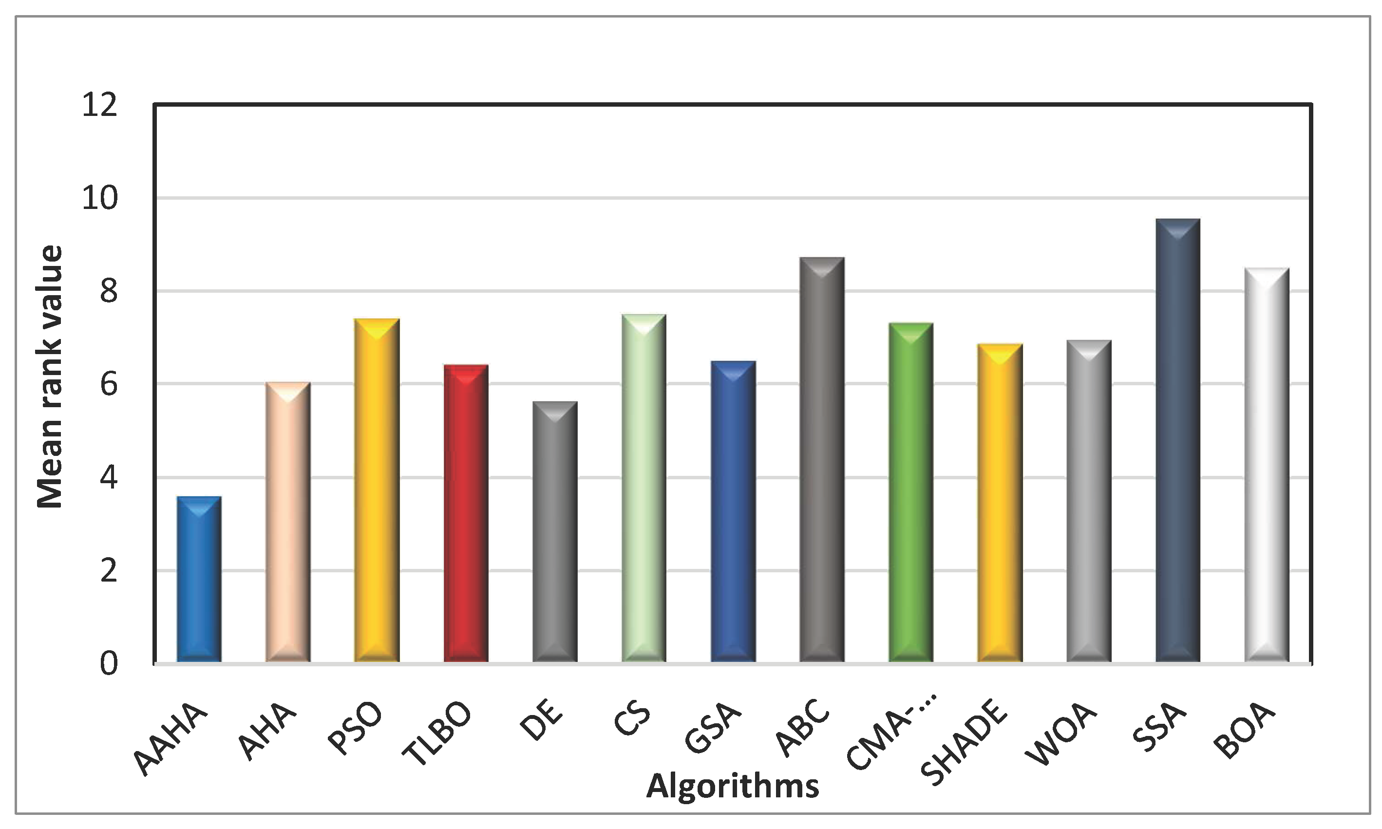
After identifying significant differences, the Holm post-hoc correction was used to pinpoint the precise algorithm pairs exhibiting these differences and to control the family-wise error rate [24]. The total rating, mean rankings, and sum of ranks for each algorithm are shown in Table 7. The Friedman test in Table 7 demonstrates that the proposed AAHA algorithm achieved the best (lowest) mean rank, which means it was the best of all the algorithms that were compared. This result confirms that it is better overall and has statistical significance in performance across the benchmark functions.
Figure 3.
Mean ranks of the comparison algorithms.
4.2.4. Friedman Aligned Ranks Test
The Friedman Aligned Ranks test is a statistical test used for comparing multiple algorithms across different problems. It builds on the standard Friedman test and is designed to increase the sensitivity of detecting differences in algorithm performance. The aligned version eliminates problem-dependent effects by first adjusting all data by aligning them to a common reference, whereas the standard Friedman test ranks methods inside each problem independently [25].
In particular, the average performance of all methods is calculated as a location metric for each problem. Then, the aligned value is calculated as the deviation from this mean for algorithm , where is the algorithm with performance on issue and is the average performance of all algorithms on that problem. After that, all the aligned values are ranked together from 1 to , creating a single global ranking as opposed to rankings for each problem [24]. The Friedman aligned ranks () test described as follows:
The results of the Friedman aligned rank in Table 8 demonstrate that the proposed AAHA algorithm had the lowest mean aligned rank, ranking it first among all algorithms. This supports the idea that it consistently outperformed the other algorithms across the benchmark functions. Table 9 shows that the Friedman Aligned Ranks test provided a p-value of 0.0281 (< 0.05), which means that there was a statistically significant difference between the algorithms that were compared. It indicates that the differences in performance are actual and not just random chance.
4.2.5. Quade Test
Like the Friedman test, the Quade test is a non-parametric multiple comparison test that assigns weights to each benchmark function based on its variability or complexity. Stated differently, issues with more significant algorithmic differences are prioritized. It is especially helpful when: Algorithm performance varies greatly depending on the problem [24,25]. Consider the relative importance of each benchmark function. The quartile means ranks of the algorithms compared for every benchmark challenge. Better overall performance is indicated by lower values, as shown in Table 10.
The Quade tests shown in Table 10 indicate that the proposed AAHA algorithm had the lowest mean rank. This means that it worked more effectively and consistently than the other algorithms across the benchmark functions.
4.2.6. Friedman Test for () Comparisons
Following the rejection of the null hypothesis using the Friedman test, pairwise comparisons were carried out using the Holm post-hoc procedure, as suggested by García et al. [24]. Through this process, the family-wise error rate (FWER) can be controlled while evaluating every conceivable pair of algorithms. The adjusted p-values produced indicate which algorithm pairs differ statistically significantly [24]. The Holm-adjusted p-values for pairwise comparisons between the proposed AAHA algorithm and the remaining algorithms are presented, with statistically significant differences (p-Holm < 0.05) highlighted in bold. The p-Holm values and significance for various optimization algorithms are shown in Table 11.
The suggested algorithm AAHA performs significantly better than CS, GSA, ABC, CMA-ES, SHADE, SSA, and BOA, while the differences with AHA, PSO, TLBO, DE, and WOA are not statistically significant, according to the Friedman post-hoc test with Holm correction (α = 0.05).
5. Conclusions
The present study provided an adaptation of the AHA to examine the effects of greater flexibility in the AHA as described in population initialization influence optimization results. The mechanism used for migration is derived from the EM-like mechanism and four initialization methods: Chaotic, Gauss. Three types of OBL, Chaotic–Sinus, Opposition-Based Learning (OBL), and Diagonal Uniform Distribution (DUD) were constructed and individually assessed. Experimental results showed that the proposed DUD initialization method achieves the best on almost all the benchmark functions, this approach achieved faster convergence and more accurate solutions as comparison to the other evaluated initialization methods. The proposed migration mechanism maintains the balance between exploitation and exploration. These results show that the optimal initial condition AHA will ensure that changes will have an important impact on overall performance without affecting the mechanism of updating. For future studies, the enhanced AHA may be applied to limited or multi-objective optimization problems, and adaptive migration control might be investigated to further improve its search balance and scalability.
Author Contributions
Conceptualization, H.N.H. and D.H.M.; methodology, H.N.H. and D.H.M.; software, H.N.H.; validation, H.N.H. and D.H.M.; formal analysis, H.N.H. and D.H.M.; investigation, H.N.H and D.H.M.; resources, H.N.H and D.H.M.; data curation, H.N.H and D.H.M.; writing—original draft preparation, H.N.H. writing—review and editing, D.H.M.; visualization, H.N.H. and D.H.M.; supervision, D.H.M.; project administration, D.H.M. All authors have read and agreed to the published version of the manuscript.
Funding
This research received no external funding.
Data Availability Statement
Data are contained within the article.
Acknowledgments
The authors would like to thank Mustansiriyah University (www.uomustansiriyah.edu.iq), Baghdad, Iraq, for its support in the present work.
Conflicts of Interest
The authors declare no conflicts of interest.
Appendix A
This section contains all the test benchmark functions used for this paper, including the search domain, category, and the global optimal solution of each function.

Table A1.
Optimization test benchmark functions.
| Category | Name of Function | Test Function | Description | Dimensions | Boundary | Optimal Value | |
| Unimodal and Separable (US) |
F1 | Stepint Function |
5 | [-100, 100] | 0 | ||
| F2 | Step Function | 30 | [-100, 100] | 0 | |||
| Unimodal and Non-separable (UN) |
F6 | Beale Function |
5 | [-4.5, 4.5] | 0 | ||
| F7 | Easom Function |
2 | [-100, 100] | -1 | |||
| F9 | Colville Function | 4 | [-10, 10] | 0 | |||
| F10 | Trid6 Function |
6 | [-36, 36] | 0 | |||
| F16 | Rosenbrock Function | 30 | [-30, 30] | 0 | |||
| Multimodal and Separable (MS) | F18 | Foxholes Function | 2 | [-65.536, 65.536] | 0 | ||
| F19 | Branin Function |
2 | [-5, 10] | 0.398 | |||
| F20 | Bohachevsky1 Function |
2 | [-100, 100] | 0 | |||
| F21 | Booth Function |
2 | [-10, 10] | 0 | |||
| F22 | Rastrigin Function | 30 | [-5.12, 5.12] | 0 | |||
| F24 | Michalewicz2 Function | 2 | [0, π] | -1.8013 | |||
|
Multimodal and Non-separable (MN) |
F27 | Schaffer Function | 2 | [-100, 100] | 0 | ||
| F28 | Six-Hump Camel Back Function | 2 | [-5, 5] | -1.0316 | |||
| F29 | Bohachevsky2 Function |
2 | [-100, 100] | 0 | |||
| F30 | Bohachevsky3 Function |
2 | [-100, 100] | 0 | |||
| F35 | Shekel7 Function | 4 | [0, 10] | -10.4029 | |||
| F39 | Hartman3 Function | 3 | [0, 1] | -3.8628 | |||
| F40 | Hartman6 Function | 6 | [0, 1] | -3.3224 | |||
| F42 | Ackley Function | 30 | [-32, 32] | 0 | |||
| F44 | Penalized2 Function | 30 | [-50, 50] | 0 | |||
| F47 | Langerman10 Function | 10 | [0, 10] | -1.4 | |||
| F48 |
|
FletcherPowell2 Function | 2 | [-100, 100] | 0 | ||
References
- Kennedy, J.; Eberhart, R. Particle Swarm Optimization. In Proceedings of the Proceedings of the IEEE International Conference on Neural Networks; IEEE: Perth, Australia, 1995; pp. 1942–1948. [Google Scholar] [CrossRef]
- Dorigo, M.; Stützle, T. Ant Colony Optimization; MIT Press: Cambridge, MA, 2004. [Google Scholar] [CrossRef]
- Karaboga, Dervis; Akay, B. A comparative study of Artificial Bee Colony algorithm. Appl. Math. Comput. 2009, 214, 108–132. [Google Scholar] [CrossRef]
- Storn, R.; Price, K. Differential Evolution-A Simple and Efficient Heuristic for Global Optimization over Continuous Spaces. J. Glob. Optim. 1997, 11, 341–359. [Google Scholar] [CrossRef]
- Zhao, W.; Wang, L.; Mirjalili, S. Artificial hummingbird algorithm: A new bio-inspired optimizer with its engineering applications. Comput. Methods Appl. Mech. Eng. 2022, 388, 114194. [Google Scholar] [CrossRef]
- Jeffrey O. Agushaka, Absalom E. Ezugwu, Laith Abualigah, and E.I.: Initialization approaches for population-based metaheuristics: A comprehensive survey and taxonomy. Appl. Sci. 2022, 12. [CrossRef]
- Malek Sarhani, Stefan Voß, and R.J.: Initialization of metaheuristics: Comprehensive review, critical analysis, and research directions. Int. Trans. Oper. Res. 2023, 30, 3361–3397. [CrossRef]
- Li, Q.; Bai, Y.; Gao, W. Improved Initialization Method for Metaheuristic Algorithms: A Novel Search Space View. IEEE Access 2021, 9, 121366–121384. [Google Scholar] [CrossRef]
- Hassanzadeh, M.R.; Keynia, F. An overview of the concepts, classifications, and methods of population initialization in metaheuristic algorithms. J. Adv. Comput. Eng. Technol. 2021, 7, 35–54. [Google Scholar]
- Cuevas, E.; Escobar, H.; Sarkar, R.; Eid, H.F. A new population initialization approach based on Metropolis–Hastings (MH) method. Appl. Intell. 2023, 53, 16575–16593. [Google Scholar] [CrossRef]
- Agushaka, J.O.; Ezugwu, A.E.; Abualigah, L.; Alharbi, S.K.; Khalifa, H.A.E.W. Efficient Initialization Methods for Population-Based Metaheuristic Algorithms: A Comparative Study; Springer Netherlands, 2023; Vol. 30. [CrossRef]
- Kuang, F.; Jin, Z.; Xu, W.; Zhang, S. A novel chaotic artificial bee colony algorithm based on Tent map. Proc. 2014 IEEE Congr. Evol. Comput. CEC 2014 2014, 235–241. [Google Scholar] [CrossRef]
- Birbil, Ş.I.; Fang, S.C. An electromagnetism-like mechanism for global optimization. J. Glob. Optim. 2003, 25, 263–282. [Google Scholar] [CrossRef]
- Tizhoosh, H.R. Opposition-Based Learning: A New Scheme for Machine Intelligence. IEEE Comput. Soc. 2005, 1, 695–701. [Google Scholar] [CrossRef]
- Xin-She Yang, S.D. Cuckoo search via Lévy flights.; 2009; pp. 210–214. [CrossRef]
- Esmat Rashedi, Hossein Nezamabadi-pour, S.S. GSA: A gravitational search algorithm. Inf. Sci. (Ny). 2009, 179, 2232–2248. [CrossRef]
- R. V. Rao, V. J. Savsani, D.P.V.: Teaching–Learning-Based Optimization: A novel method for constrained mechanical design. Comput. Des. 2011, 43, 303–315. [CrossRef]
- Hansen, Nikolaus; Ostermeier, A. Completely derandomized self-adaptation in evolution strategies. Evol. Comput. 2001, 9, 159–195. [Google Scholar] [CrossRef] [PubMed]
- Faris;, S.M.A.H.G.S.Z.M.S.S.H.: Salp Swarm Algorithm: A bio-inspired optimizer for engineering design problems. Adv. Eng. Softw. 2017, 114, 163–191. [CrossRef]
- Seyedali Mirjalili, A.L. The Whale Optimization Algorithm. Adv. Eng. Softw. 2016, 95, 51–67. [Google Scholar] [CrossRef]
- Fukunaga, R.T.A. Success-history based parameter adaptation for Differential Evolution. 2013 IEEE Congr. 2013 IEEE Congr. Evol. Comput. 2013, 71–78. [Google Scholar] [CrossRef]
- Sankalap Arora, S.S. Butterfly Optimization Algorithm: A novel approach for global optimization. Soft Comput. 23, 715–734. [CrossRef]
- Derrac, J.; García, S.; Molina, D.; Herrera, F. A practical tutorial on the use of nonparametric statistical tests as a methodology for comparing evolutionary and swarm intelligence algorithms. Swarm Evol. Comput. 2011, 1, 3–18. [Google Scholar] [CrossRef]
- García, S.; Fernández, A.; Luengo, J.; Herrera, F. Advanced nonparametric tests for multiple comparisons in the design of experiments in computational intelligence and data mining: Experimental analysis of power. Inf. Sci. (Ny). 2010, 180, 2044–2064. [Google Scholar] [CrossRef]
- García, Salvador; Molina, Daniel; Lozano, Manuel; Herrera, F.: A study on the use of non-parametric tests for analyzing the evolutionary algorithms’ behaviour: a case study on the CEC’2005 special session on real parameter optimization. J. Heuristics 2009, 15, 617–644. [CrossRef]
Figure 1.
Flowchart of the Proposed AAHA.
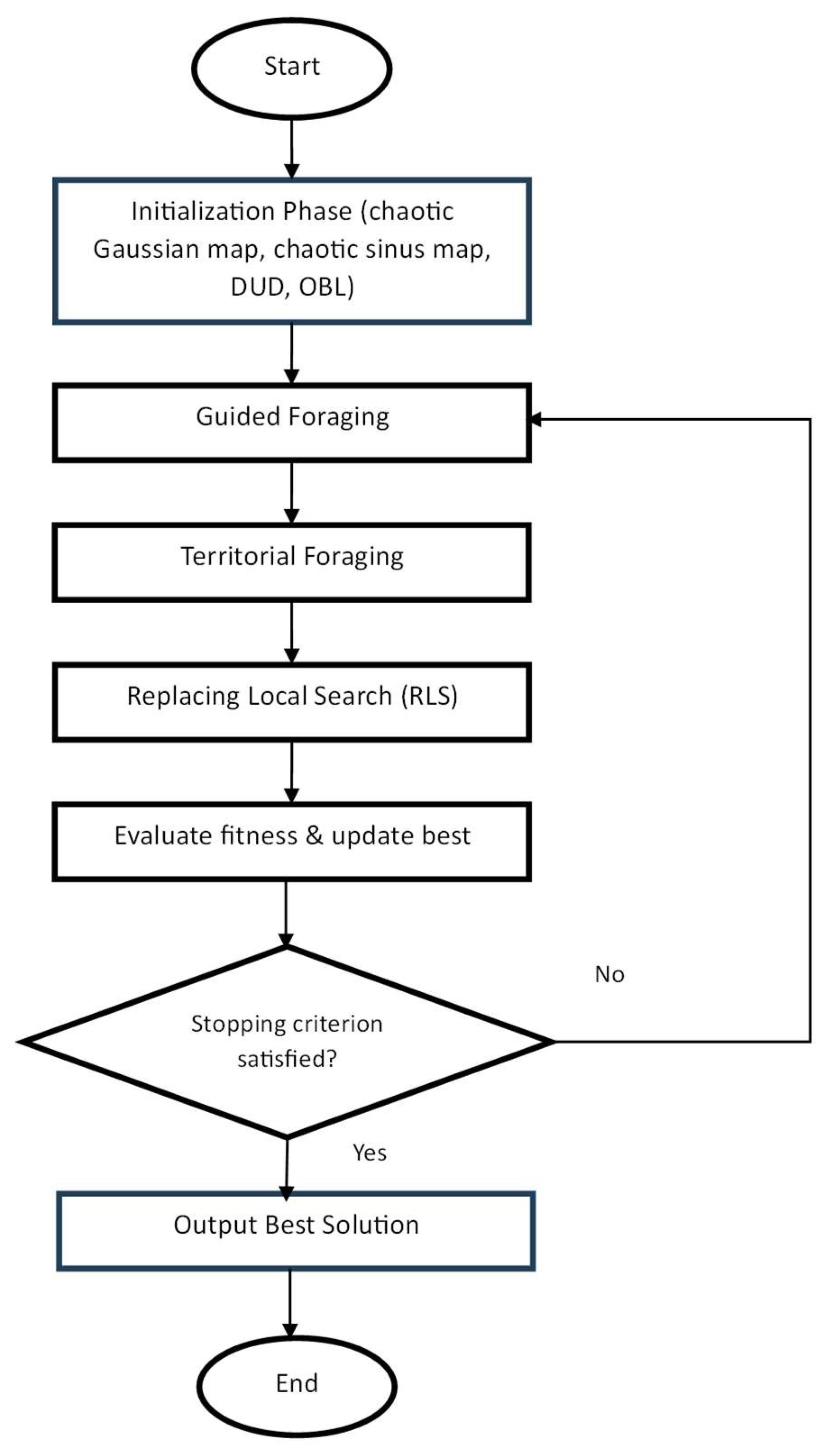
Figure 2.
Convergence performance comparison between AHA and AAHA algorithms for selected benchmark functions.
Figure 2.
Convergence performance comparison between AHA and AAHA algorithms for selected benchmark functions.

Table 1.
The and values for AHA under various initialization approaches for 2 test functions.
| Function | Initialization approaches | |||||||
|---|---|---|---|---|---|---|---|---|
| Gauss | Sine | DUD | BUL | |||||
| F1 | -5 | 0 | -5 | 0 | -5 | 0 | -5 | 0 |
| F2 | 0 | 0 | 0 | 0 | 0 | 0 | 0 | 0 |
| F6 | 0 | 0 | 0 | 0 | 0 | 0 | 0 | 0 |
| F7 | -1 | 0 | -1 | 0 | -1 | 0 | -1 | 0 |
| F9 | 1.0366E-06 | 5.6601E-06 | 9.1862E-26 | 4.8953E-25 | 2.48E-27 | 1.3458E-26 | 2.2803E-21 | 1.2489E-20 |
| F10 | -50 | 7.9255E-14 | -50 | 5.0863E-14 | -50 | 2.293E-14 | -50 | 4.8047E-14 |
| F16 | 24.9025 | 0.1977 | 24.7425 | 0.39202 | 15.8206 | 0.18236 | 24.9495 | 12.0955 |
| F18 | 0.998003 | 0 | 0.998003 | 0 | 0.998003 | 0 | 0.998003 | 0 |
| F19 | 0.397887 | 0 | 0.397887 | 0 | 0.397887 | 0 | 0.397887 | 0 |
| F20 | 0 | 0 | 0 | 0 | 0 | 0 | 0 | 0 |
| F21 | 0 | 0 | 0 | 0 | 0 | 0 | 0 | 0 |
| F22 | 0 | 0 | 0 | 0 | 0 | 0 | 0 | 0 |
| F24 | −1.801303 | 9.03E-16 | −1.801303 | 9.03E-16 | −1.801303 | 9.03E-16 | −1.801303 | 9.03E-16 |
| F27 | 0 | 0 | 0 | 0 | 0 | 0 | 0 | 0 |
| F28 | −1.031628 | 6.65E-16 | −1.031628 | 6.65E-16 | −1.031628 | 6.65E-16 | −1.031628 | 6.65E-16 |
| F29 | 0 | 0 | 0 | 0 | 0 | 0 | 0 | 0 |
| F30 | 0 | 0 | 0 | 0 | 0 | 0 | 0 | 0 |
| F35 | -10.40294 | 1.44E-15 | -10.40294 | 3.2986E-16 | -10.40294 | 0 | -10.40294 | 2.322E-15 |
| F39 | −3.862782 | 2.71E-15 | −3.862782 | 2.71E-15 | −3.862782 | 2.71E-15 | −3.862782 | 2.71E-15 |
| F40 | -3.3144 | 0.030244 | -3.3184 | 0.021764 | -3.3224 | 5.15E-16 | -3.3144 | 0.030244 |
| F42 | 8.88E−16 | 0 | 8.88E−16 | 0 | 8.88E−16 | 0 | 8.88E−16 | 0 |
| F44 | 2.3076E-07 | 1.7294E-07 | 3.117E-07 | 8.6637E-07 | 7.5269E-08 | 7.5985E-08 | 2.0513E-07 | 1.1722E-07 |
| F47 | -3.5982 | 0.31429 | -3.5408 | 0.43675 | -3.6556 | 1.7726E-06 | -3.5982 | 0.3143 |
| F48 | 0 | 0 | 0 | 0 | 0 | 0 | 0 | 0 |
Table 2.
Comparisons of various algorithms’ outcomes for various benchmark functions.
| Function | Index | AAHA | AHA | PSO | TLBO | DE | CS | GSA | ABC | CMA-ES | SHADE | WOA | SSA | BOA |
|---|---|---|---|---|---|---|---|---|---|---|---|---|---|---|
| F1 |
-50 | -50 | -1.66667 0.660895 |
-4.966667 0.182574 |
-50 | -50 | -1.7 0.466092 |
-50 | -0.46667 1.33218 |
-4.23333 2.9206 |
-50 | -3.66667 0.711116 |
-2 1.94759 |
|
| F2 |
Mean | 00 | 00 | 0.066667 0.253721 |
00 | 0.333333 0.844183 |
36.3 10.299481 |
00 | 4.966667 1.449931 |
00 | 00 | 00 | 5.13333 2.93297 |
00 |
| Std | ||||||||||||||
| F6 |
Mean | 00 | 00 | 00 | 00 | 00 | 1.36E-17 3.92E-17 |
4.94E-28 1.90E-27 |
1.85E-14 4.09E-14 |
00 | 1.13E-27 4.30E-27 |
7.11E-14 4.21E-14 |
4.00E-16 3.48E-16 |
1.47E-05 1.43E-05 |
| Std | ||||||||||||||
| F7 |
Mean | -10 | -10 | -10 | -10 | -10 | -1 1.75E-13 |
-0.96667 0.182574 |
-1 6.31E-12 |
-10 | -0.20236 0.40574 |
-1 1.02E-10 |
-1 2.30E-13 |
-0.99999 4.69E-06 |
| Std | ||||||||||||||
| F9 |
Mean | 2.4789E-27 1.3458E-26 |
2.83E-24 2.52E-24 |
7.63E-03 6.49E-03 |
9.99E-08 2.26E-05 |
3.84E-06 2.10E-05 |
1.19E-02 2.04E-02 |
0.697872 0.933509 |
4.62E-02 5.35E-02 |
5.81E-24 3.18E-24 |
1.23E-06 1.69E-06 |
0.15092 0.104465 |
1.52E-10 2.06E-10 |
9.11E-02 9.24E-02 |
| Std | ||||||||||||||
| F10 |
Mean | -50 2.293E-14 |
-50 6.53E-14 |
-50 2.96E-14 |
-50 2.47E-14 |
-50 2.89E-14 |
-50 2.67E-10 |
-50 1.36E-14 |
-50 1.73E-05 |
-50 3.95E-14 |
-50 5.72E-14 |
-50 7.90E-08 |
-50 3.94E-12 |
-50 4.60E-03 |
| Std | ||||||||||||||
| F16 |
Mean | 15.8206 0.18236 |
25.065057 0.278139 |
49.164576 30.081342 |
23.377421 0.703925 |
23.88551 23.616923 |
784.63745 271.3126 |
26.00923 0.201436 |
8717.4121 28778.6436 |
25.95142 33.08219 |
26.06047 0.32561 |
25.119595 0.2677 |
48.64191 48.27414 |
28.668781 3.10E-02 |
| Std | ||||||||||||||
| F18 |
Mean | 0.9980 | 0.9980030 | 0.9980030 | 0.9980030 | 0.998004 2.19E-15 |
3.638354 2.217956 |
0.998138 5.61E-04 |
3.00695 2.4873 |
0.9980030 | 0.998003 1.36E-13 |
0.998003 1.82E-16 |
0.998003 5.42E-08 |
0.9980030 |
| Std | ||||||||||||||
| F19 |
Mean | 0.3978870 | 0.3978870 | 0.3978870 | 0.3978870 | 0.3978870 | 0.397887 2.65E-14 |
0.3978870 | 0.397887 7.36E-09 |
0.400 | 0.44 9.18E-02 |
0.397887 1.72E-09 |
0.40 2.88E-15 |
0.40 2.63E-05 |
| Std | ||||||||||||||
| F20 |
Mean | 00 | 00 | 00 | 00 | 00 | 00 | 00 | 5.10E-10 5.13E-10 |
00 | 61.90491 102.66111 |
00 | 3.52E-12 4.70E-12 |
00 |
| Std | ||||||||||||||
| F21 | Mean | 00 | 00 | 00 | 00 | 00 | 1.38E-23 2.71E-23 |
1.79E-20 2.19E-20 |
2.36E-10 3.25E-10 |
00 | 00 | 4.19E-07 3.25E-07 |
2.52E-15 3.27E-15 |
5.59E-06 6.65E-06 |
| Std | ||||||||||||||
| F22 | Mean | 00 | 00 | 30.845624 7.6342136 |
12.679728 5.5850898 |
153.2381 32.147688 |
109.4123 13.43076 |
14.6259 3.265065 |
188.6345 12.28813 |
165 8.99333 |
115 9.03763 |
00 | 33.79541 14.36489 |
5.79935 31.76315 |
| Std |
Table 3.
comparisons of the optimization outcomes for other benchmark functions.
| Function | Index | AAHA | AHA | PSO | TLBO | DE | CS | GSA | ABC | CMA-ES | SHADE | WOA | SSA | BOA |
|---|---|---|---|---|---|---|---|---|---|---|---|---|---|---|
| F24 |
−1.801303 9.03E-16 |
-1.801303 9.03E-16 |
-1.801303 9.03E-16 |
-1.801303 9.03E-16 |
-1.801303 9.03E-16 |
-1.801303 9.03E-16 |
-1.801303 9.53E-16 |
-1.801303 2.82E-15 |
-1.80127 1.79E-04 |
-1.801303 9.03E-16 |
-1.801303 1.57E-10 |
-1.801303 7.49E-15 |
-1.801206 1.48E-04 |
|
| F27 |
Mean | 00 | 00 | 00 | 00 | 00 | 6.40E-12 2.56E-11 |
1.12E-02 1.24E-02 |
3.99E-06 5.31E-06 |
00 | 5.97E-03 3.24E-02 |
00 | 1.41E-16 2.57E-16 |
00 |
| Std | ||||||||||||||
| F28 |
Mean | −1.031628 6.65E-16 |
-1.031628 6.65E-16 |
-1.031628 6.78E-16 |
-1.031628 6.78E-16 |
-1.031628 6.78E-16 |
-1.031628 5.13E-16 |
-1.031628 5.68E-16 |
-1.031628 7.78E-11 |
-1.03163 6.78E-16 |
-1.03163 6.71E-16 |
-1.03163 1.77E-14 |
-1.03163 1.56E-15 |
-1.03163 1.87E-06 |
| Std | ||||||||||||||
| F29 |
Mean | 00 | 00 | 00 | 00 | 00 | 00 | 00 | 2.92E-09 3.50E-09 |
3.91E-02 0.21426 |
79.93775 110.07691 |
00 | 2.63E-12 2.95E-12 |
1.85E-17 2.66E-17 |
| Std | ||||||||||||||
| F30 |
Mean | 00 | 00 | 00 | 00 | 00 | 00 | 00 | 3.46E-07 3.63E-07 |
00 | 00 | 00 | 1.18E-12 1.38E-12 |
00 |
| Std | ||||||||||||||
| F35 |
Mean | −10.402940 | -10.40294 1.44E-15 |
-9.87415 1.613482 |
-10.22344 0.983192 |
-10.40294 1.68E-15 |
-10.40294 1.39E-06 |
-10.40294 6.60E-16 |
-10.40294 1.27E-13 |
-7.41732 1.92462 |
-10.40294 9.90E-16 |
-10.40294 1.23E-05 |
-9.82871 1.76503 |
-10.29099 7.29E-02 |
| Std | ||||||||||||||
| F39 |
Mean | −3.862782 2.71E-15 |
−3.862783 2.71E-15 |
−3.862784 2.71E-15 |
−3.862785 2.71E-15 |
−3.862786 2.71E-15 |
−3.862787 2.71E-15 |
−3.862788 2.71E-15 |
−3.862789 2.71E-15 |
−3.862790 2.71E-15 |
−3.862791 2.71E-15 |
−3.862792 2.71E-15 |
−3.862793 2.71E-15 |
−3.862794 2.71E-15 |
| Std | ||||||||||||||
| F40 |
Mean | -3.3224 5.15E-16 |
-3.310106 3.63E-02 |
-3.254622 5.99E-02 |
-3.318032 2.17E-02 |
-3.302181 4.51E-02 |
-3.321997 4.69E-07 |
-3.322 1.36E-15 |
-3.322 4.80E-15 |
-3.30989 3.69E-02 |
-3.322 1.36E-15 |
-3.2542 6.04E-02 |
-3.27337 6.06E-02 |
-3.30731 1.19E-02 |
| Std | ||||||||||||||
| F42 |
Mean | 8.88E−160 | 8.88E-160 | 9.97E-02 0.380955 |
6.57E-15 1.77E-15 |
3.99E-08 1.85E-08 |
9.189665 1.819592 |
3.38E-09 4.02E-10 |
0.655145 0.216113 |
8.86E-06 2.60E-06 |
3.55E-04 7.07E-05 |
2.90E-15 2.22E-15 |
1.2144 0.97792 |
3.63E-07 7.41E-08 |
| Std | ||||||||||||||
| F44 |
Mean | 7.5269E-08 7.5985E-08 |
0.669596 0.547843 |
7.69E-03 1.45E-02 |
4.26E-02 4.90E-02 |
1.47E-03 3.80E-03 |
7.714342 2.177475 |
2.17E-18 5.70E-19 |
5657.875 5582.683 |
5.98E-10 4.54E-10 |
4.91E-07 2.30E-07 |
1.94E-03 8.19E-03 |
2.93E-03 4.94E-03 |
4.17E-01 1.40E-01 |
| Std | ||||||||||||||
| F47 | Mean | -3.6556 1.7726E-06 |
-0.568135 0.203332 |
-0.662263 0.181552 |
-0.605597 0.270130 |
-1.128604 0.405098 |
-0.75937 9.88E-02 |
-0.10345 0.111923 |
-1.09223 0.233308 |
-0.73411 0.3812 |
-1.16257 0.28561 |
-0.35923 0.15903 |
-0.49452 0.26391 |
-0.19268 9.87E-02 |
| Std | ||||||||||||||
| F48 | Mean | 00 | 00 | 00 | 00 | 00 | 2.30E-13 4.49E-13 |
2.51E-17 2.15E-17 |
3.80E-10 7.57E-10 |
0.21623 0.69008 |
17.16006 25.83799 |
1.60E-11 5.57E-11 |
8.10E-13 8.72E-13 |
4.96E-03 5.06E-03 |
| Std |
Table 4.
Nonparametric statistical procedures used in this work.
| Type of comparison | Procedures | Subsection |
|---|---|---|
| Pairwise comparisons | Sign test | 4.2.1 |
| Multiple comparisons (1 × ) | Multiple sign test Friedman test Friedman Aligned ranks Quade test |
4.2.2 4.2.3 4.2.4 4.2.5 |
| Multiple comparisons () | Friedman test | 4.2.6 |
Table 5.
Results of pairwise comparisons using the sign test.
| AAHA | AHA | PSO | TLBO | DE | CS | GSA | ABC | CMA-ES | SHADE | WOA | SSA | BOL |
|---|---|---|---|---|---|---|---|---|---|---|---|---|
| Wins (+) | 7 | 12 | 11 | 10 | 14 | 14 | 17 | 13 | 17 | 11 | 19 | 19 |
| Loses (−) | 0 | 0 | 0 | 0 | 0 | 1 | 0 | 2 | 1 | 1 | 1 | 1 |
Table 6.
Multiple sign test results contrast the AAHA with the other algorithms.
| Algorithm | Wins (+) | Losses (−) | Ties | Detected differences | ||
|---|---|---|---|---|---|---|
| AHA | 7 | 0 | 17 | 7 | 0.015625 | α = 0.05 |
| PSO | 12 | 0 | 12 | 12 | 0.000488 | α = 0.05 |
| TLBO | 11 | 0 | 13 | 11 | 0.000977 | α = 0.05 |
| DE | 10 | 0 | 14 | 10 | 0.001953 | α = 0.05 |
| CS | 14 | 0 | 10 | 14 | 0.000122 | α = 0.05 |
| GSA | 14 | 1 | 9 | 15 | 0.000977 | α = 0.05 |
| ABC | 17 | 0 | 7 | 17 | 0.000015 | α = 0.05 |
| CMA-ES | 13 | 2 | 9 | 15 | 0.007385 | α = 0.05 |
| SHADE | 17 | 1 | 6 | 18 | 0.000145 | α = 0.05 |
| WOA | 11 | 1 | 12 | 12 | 0.006348 | α = 0.05 |
| SSA | 19 | 1 | 4 | 20 | 0.000040 | α = 0.05 |
| BOA | 19 | 1 | 4 | 20 | 0.000040 | α = 0.05 |
Table 7.
Friedman tests for every algorithm under comparison.
| AAHA | AHA | PSO | TLBO | DE | CS | GSA | ABC | CMA-ES | SHADE | WOA | SSA | BOA | |
|---|---|---|---|---|---|---|---|---|---|---|---|---|---|
| Sum of ranks | 90.5 | 124 | 171 | 138.5 | 144 | 185.5 | 178 | 216.5 | 174 | 176 | 160.5 | 208.5 | 217 |
| Mean of ranks | 3.771 | 5.167 | 7.125 | 5.771 | 6 | 7.729 | 7.417 | 9.021 | 7.25 | 7.333 | 6.688 | 8.688 | 9.042 |
| Overall Rank | 1 | 2 | 6 | 3 | 4 | 8 | 10 | 13 | 7 | 9 | 5 | 11 | 12 |
Table 8.
Friedman Aligned Ranks of the algorithms.
| Algorithm | Mean aligned rank | Rank |
|---|---|---|
| AAHA | 122.958333 | 1 |
| AHA | 133.020833 | 2 |
| TLBO | 133.791667 | 3 |
| DE | 143.312500 | 4 |
| WOA | 144.250000 | 5 |
| PSO | 155.187500 | 6 |
| BOA | 160.208333 | 7 |
| GSA | 161.770833 | 8 |
| CMA-ES | 171.145833 | 9 |
| SSA | 171.645833 | 10 |
| ABC | 176.812500 | 11 |
| CS | 176.895833 | 12 |
| SHADE | 183.500000 | 13 |
Table 9.
Friedman Aligned Ranks test summary.
| Statistic | df | p-value | Decision (α = 0.05) |
|---|---|---|---|
| χ2_FA | 12 | 0.0281 | Significant |
Table 10.
Quade’s mean ranks of the compared algorithms.
| Algorithm | Quade’s mean rank | Rank |
|---|---|---|
| AAHA | 3.7708 | 1 |
| AHA | 5.1667 | 2 |
| TLBO | 5.7708 | 3 |
| DE | 6.0000 | 4 |
| WOA | 6.6875 | 5 |
| PSO | 7.1250 | 6 |
| CMA-ES | 7.2500 | 7 |
| SHADE | 7.3333 | 8 |
| GSA | 7.4167 | 9 |
| CS | 7.7292 | 10 |
| SSA | 8.6875 | 11 |
| ABC | 9.0208 | 12 |
| BOA | 9.0417 | 13 |
Table 11.
Friedman post-hoc comparison results (Holm correction, α = 0.05).
| Algorithm | p-Holm | Significance |
|---|---|---|
| AHA | 1.0000 | No |
| PSO | 0.0542 | No |
| TLBO | 1.0000 | No |
| DE | 1.0000 | No |
| CS | 0.0020 | Yes |
| GSA | 0.0061 | Yes |
| ABC | 0.0000 | Yes |
| CMA-ES | 0.0261 | Yes |
| SHADE | 0.0121 | Yes |
| WOA | 0.2500 | No |
| SSA | 0.0000 | Yes |
| BOA | 0.0000 | Yes |
Disclaimer/Publisher’s Note: The statements, opinions and data contained in all publications are solely those of the individual author(s) and contributor(s) and not of MDPI and/or the editor(s). MDPI and/or the editor(s) disclaim responsibility for any injury to people or property resulting from any ideas, methods, instructions or products referred to in the content. |
© 2025 by the authors. Licensee MDPI, Basel, Switzerland. This article is an open access article distributed under the terms and conditions of the Creative Commons Attribution (CC BY) license (http://creativecommons.org/licenses/by/4.0/).
Copyright: This open access article is published under a Creative Commons CC BY 4.0 license, which permit the free download, distribution, and reuse, provided that the author and preprint are cited in any reuse.


