
Submitted:
23 November 2025
Posted:
24 November 2025
You are already at the latest version
Abstract
We study a minimum-time (time-optimal) control problem for a nonlinear pendulum-type oscillator, in which the control input is the system’s natural frequency constrained to a prescribed interval. The objective is to transfer the oscillator from a given initial state to a prescribed terminal state in the shortest possible time. Our approach combines Pontryagin’s maximum principle with Bellman’s principle of optimality. First, we decompose the original problem into a sequence of auxiliary problems, each corresponding to a single semi-oscillation. For every such subproblem, we obtain a complete analytical solution by applying Pontryagin’s maximum principle. These results allow us to reduce the global problem of minimizing the transfer time between the prescribed states to a finite-dimensional optimization problem over a sequence of intermediate amplitudes, which is then solved numerically by dynamic programming. Numerical experiments reveal characteristic features of optimal trajectories in the nonlinear regime, including a non-periodic switching structure, non-uniform semi-oscillation durations, and significant deviations from the behavior of the corresponding linearized system. The proposed framework provides a basis for the synthesis of fast oscillatory regimes in systems with controllable frequency, such as pendulum and crane systems and robotic manipulators.
Keywords:
optimal control
; harmonic oscillator
; Bellman optimality principle
; Pontryagin maximum principle
MSC: 49J15
1. Introduction
Minimizing the duration of transient processes in mechanical and oscillatory systems is one of the fundamental problems of modern control theory. Classical optimal control methods, developed within the framework of Pontryagin’s maximum principle and dynamic programming [1,2,3,4], provide a rigorous theoretical foundation for studying the structure of optimal controls. However, their direct application to nonlinear oscillators with bounded parametric control is highly nontrivial.
A large class of contemporary applied problems is associated with swing suppression and fast load transportation in crane systems. In recent years, a wide range of highly efficient command-shaping and active vibration suppression methods has been developed. In particular, [5,6] proposes optimization-based input-shaping and MPC-based control algorithms for overhead cranes. Enhanced swing-suppression strategies, such as Negative Zero-Vibration schemes and low-pass-filter-based methods, are studied in [7,8]. Phase-planning and optimal anti-sway methods for tower and container cranes are presented in [9,10,11]. These results show that controlling the frequency or parameters of the oscillatory dynamics is a key mechanism for accelerating motion while maintaining stability.
In parallel, there has been active development in the analytical and semi-analytical study of nonlinear oscillators. Methods for estimating periods and frequencies, models with fractal–fractional operators, and various refinements of He’s frequency formulation are analyzed in [12,13,14]. Robust and optimal control methods for fractional nonlinear models are presented in [15], while modern variational and Hamiltonian-based computational techniques are discussed in [16]. Despite their high accuracy in describing the dynamics, these approaches generally do not yield a fully analytical solution to the minimum-time problem for nonlinear pendulums with a bounded controllable frequency.
Significant progress has also been achieved in dynamic programming and adaptive dynamic programming (ADP), including value-iteration and constrained-cost schemes for nonlinear systems [17,18]. Applications of ADP to systems with state delays are presented in [19]. Classical works on ADP and reinforcement-learning-based optimal control [20,21] provide powerful numerical tools for solving constrained optimal control problems; however, they do not supply explicit analytical switching conditions either.
Modern optimal control techniques are particularly in demand in power systems, mechatronics, and space engineering. Applications of Neural ODE methods to frequency stabilization in power systems are investigated in [22]; nonlinear frequency regulation in microgrids is studied in [23]; and swing suppression in flexible space structures is addressed in [24]. These directions demonstrate a growing interest in controlling oscillator-like parameters in complex real-world systems.
For linear harmonic systems with parametric excitation and viscous friction, rigorous analytical solutions for the structure of optimal controls have been obtained in [25,26]. However, linear models do not capture all the characteristic features inherent to pendulum-type systems.
Thus, there is a gap between, on the one hand, the highly developed swing-suppression methods for quasi-linear models [5,6,7,8], analytical and semi-empirical techniques for nonlinear oscillators [12,13,14,15,16], and numerical ADP/MPC-based methods [17,18,21,22], and, on the other hand, the absence of a strict analytical solution to the minimum-time control problem for a nonlinear pendulum when the frequency acts as the control parameter.
The aim of this work is to help fill this gap. We consider a nonlinear pendulum-type oscillator whose natural frequency, varying within a prescribed range, serves as the control input, and we study the problem of minimizing the transfer time between two rest states. Based on Pontryagin’s maximum principle and Bellman’s principle of optimality, we rigorously decompose the motion into semi-oscillations, show that the optimal control on each semi-oscillation is bang–bang with at most two switchings, derive analytical formulas for the semi-oscillation duration and switching conditions, and finally reduce the global problem to a finite-dimensional optimization problem.
The structure of the paper is as follows. Section 2 formulates the problem statement. Section 3 is devoted to deriving the structure of the optimal control on a single semi-oscillation. Section 4 investigates the conditions for the existence of a solution and provides analytical expressions for the optimal time. Section 5 constructs the global minimum-time trajectory using Bellman’s principle and presents numerical results together with a comparison to the linear system. The conclusions discuss possible directions for further development of the model.
2. Problem Statement
We consider a nonlinear pendulum-type oscillator with a time-varying natural frequency serving as the control input. Its dynamics are described by
where is the angular displacement (state coordinate), is the angular velocity, and is the (unknown) final time of motion.
The control input is the frequency function , which is subject to the bounds
where and are fixed constants.
The initial and terminal states are specified by
where and . The point is an equilibrium of system (1) for any admissible frequency , since the control enters the equation multiplicatively. Hence a direct transfer through the equilibrium state is impossible and is not considered.
The goal of the study is to transfer the system from the initial state to the terminal state, defined in (3), in minimal time, subject to the constraint (2). The quantities to be determined are the optimal terminal time T and the optimal control . Collecting all conditions together, we arrive at the following minimum-time optimal control problem:
In what follows, we restrict attention to solutions satisfying
This assumption rules out phase wrapping (slipping), so that the equilibrium position remains at .
To solve problem (4), we adopt an approach analogous to that used in [25,26] for optimal control of a linear oscillator. Exploiting the oscillatory nature of the optimal trajectory, the optimal control problem is decomposed into a sequence of similar subproblems, each corresponding to a single semi-oscillation of the optimal trajectory. First, using Pontryagin’s maximum principle [1], we solve the problem for one semi-oscillation. Then, by applying the dynamic programming method [4], we obtain a solution to the global problem.
3. Optimal Control on a Single Semi-Oscillation
Exploiting the oscillatory nature of the trajectories of system (4) for any admissible control and the symmetry with respect to the origin in the phase plane, we decompose the global motion into separate semi-oscillations. By Bellman’s principle of optimality, each semi-oscillation of a globally optimal trajectory must itself be optimal for an appropriately posed two-point boundary-value problem.
In this section, we introduce such an auxiliary problem corresponding to a single semi-oscillation and formulate it as a minimum-time optimal control problem.
We consider a motion that starts at rest at a positive angular displacement and ends at rest at a negative angular displacement, with strictly decreasing angle along the way. This corresponds to one semi-oscillation of the pendulum-like system and leads to the following auxiliary minimum-time optimal control problem:
The monotonicity condition ensures that is strictly decreasing on and indeed describes a single semi-oscillation from the amplitude A to the amplitude B. In other words, the trajectory passes from a right-hand rest position to a left-hand rest position without any additional turning points.
The boundary conditions in (5) prescribe both the coordinate and the velocity at the endpoints (here, zero velocity). They play a crucial role for two reasons:
- They guarantee that individual semi-oscillations can be smoothly concatenated into a single global trajectory of problem (4), with continuity of both state and velocity at the junction points.
Thus, understanding the optimal control for the auxiliary problem (5) is a central step in solving the global minimum-time problem (4). In the next section, we apply Pontryagin’s maximum principle to (5), derive the structure of the optimal control on a single semi-oscillation, and determine the admissible bang–bang switching patterns.
4. Application of Pontryagin’s Maximum Principle to the Single Semi-Oscillation Problem
We apply Pontryagin’s maximum principle [1] to problem (5). To this end, we introduce the notation and rewrite (5) as a system of first-order differential equations:
We write the Pontryagin function:
and denote its upper boundary:
According to PMP if , , and constitute a solution to the optimal control problem (6), then the following three conditions are satisfied:
- (I)
- There exist continuous functions and , which never simultaneously become zero and are solutions to the adjoint system:
- (II)
- For any , the maximum condition is satisfied:
- (III)
- For any , a specific inequality occurs:
Let us show that the case of singular control in Formula (9), specifically when over a non-zero length interval of time, is impossible, assuming the opposite. This means considering the existence of a time interval during which . In such an interval, determining the value of optimal control from the maximum condition would not be feasible.
Given the continuity of the functions and , it is possible either for over some interval or for over a certain time period.
If , then must also be, identically, zero. However, this conclusion, derived from the second equation of the adjoint system (7), implies that , contradicting the maximum principle’s condition (I).
In the scenario where , it follows that . Such a case is deemed impossible, as it contradicts the condition .
This reasoning leads to the formulation of a statement:
Optimal control is limited to only two values, and , dictated by the sign of the product . Considering the case where this product equals zero as non-existent is justified by the fact that the control value at a single point or a finite number of points lacks any impact on the trajectory of the controlled system.
Now, we consider condition (III). It represents the greatest interest at values and .
At , the condition is expressed as
At , the condition becomes
Given the boundary conditions that , and considering that the control value is always positive, with and , the following additional conditions are derived from (10) and (11)
We now investigate the number of possible switching points of the optimal control. From formula (9) we see that a switching is only possible at points where either or . On a single semi-oscillation, the trajectory crosses zero exactly once. We therefore study the function and determine the maximal possible number of its zeros on the interval . Combining system (5) with the adjoint system (7), we obtain the following system of two differential equations, which governs the adjoint variable :
We will show that, on any interval where keeps a constant sign, the function can have at most one zero. Assume the contrary, and suppose that there exist at least two points at which vanishes (see Figure 1). In the absence of switchings, the control is constant, and the solution of the first equation of system (13) is a periodic function. Consider an interval of length equal to half of this period, bounded by two consecutive zeros of (for the auxiliary optimal control problem, we are in fact interested in an even shorter interval, corresponding to one quarter of the period). Note that the second equation of system (13) can also be regarded as an oscillation equation with a time-varying frequency determined by . Accordingly, the minimal distance between consecutive zeros of is achieved at the maximal frequency, that is, at the maximal value of the coefficient (see Sturm–Picone comparison theorem [27]), which corresponds to the minimal possible value of . This implies that, in order to attain the minimal distance between zeros of , its first zero must coincide with a zero of , as shown in Figure 1. This configuration corresponds to the following Cauchy problem:
Note that the condition follows from the symmetry of the first equation with respect to the point and the evenness of the function , while the condition follows from the possibility of normalizing the adjoint variable.
We also note that we are interested in an interval where the control keeps a constant sign. In this case, by the time rescaling one can eliminate from the equations, so we may assume . Hence system (14) depends only on a single unknown parameter . We now study this dependence.
Let denote the first nonzero instant such that , and let denote the first nonzero instant such that (see Figure 1). We compute these quantities as functions of by numerically solving the Cauchy problem (14) and plotting the resulting dependencies.
The numerical results in Figure 2 show that the configuration depicted in Figure 1 is impossible, since the distance between consecutive zeros of is always larger than the distance between consecutive zeros of . Moreover, both distances tend to as , because in this limit the dynamics approach those of the corresponding linear system, for which these distances are equal [25,26]. For larger values of (specifically ) one observes a transition from oscillatory to rotational motion, which is incompatible with the constraint .
Thus, we have shown that in problem (5) the optimal control can have at most one switching in each region where keeps a constant sign, and therefore at most three switchings in total (two at zeros of and one at the zero of ).
Furthermore, the case of three switchings is also impossible: in that situation we would have and , and from conditions (9) and (12) it follows that the optimal control near the initial and terminal segments must take the same value , which contradicts the odd number of switchings.
As a result, taking into account conditions (12), we conclude that the optimal control on a single semi-oscillation can only have one of the patterns shown in Figure 3. The remaining three control types, which do not satisfy all the conditions of the maximum principle, are depicted in Figure 4. Note that this selection of admissible control patterns coincides with the problem studied in [25,26], since the signs of and coincide on the interval .
We have determined the structure of the optimal control on a single semi-oscillation. It remains to identify for which boundary conditions problem (5) admits a solution, and which control type corresponds to the given boundary values.
5. Existence of Solution for One Semi-Oscillation
Let us consider the question of the existence of a solution for one semi-oscillation, i.e., for which boundary values there exists a control that transfers the system from the initial state to the final state in one semi-oscillation.
We transform the first equation of problem taking into account that the control is a piecewise constant function. On an interval where the control is constant, we multiply the equation by :
Noting that and , we obtain the equation:
Integrating the last equation with , we have:
Integrating the obtained equation once more on any interval where the control is constant, we arrive at an expression for time in terms of an elliptic integral (see [28]):
Here we have a minus sign because the function is decreasing. Note also that the function is the upper limit of the elliptic integral, which cannot be evaluated analytically.
The constant h in (15) is determined from the differentiability condition of the function for and the satisfaction of the boundary conditions.
Now, based on what has been said, we determine the missing parameter values (the constant in (15), the switching points ) for the optimal control and optimal trajectory. Let us first consider control type 4 from Figure 3, which also includes type 3 when and type 5 when In this case, the optimal control has the form:
where the switching points and are unknown; it is only known that .
Next, using the form of control (17) and the boundary conditions from (5), we determine the values of the constant h in equation on each interval where the control is constant:
- On the interval we have:
- On the interval we have:
-
On the interval , using the condition , and the continuity and differentiability of the function at the switching points, we have the system:Denoting we write the solution of system (18) in the form:Note that the switching moment is defined implicitly by the second equation of system (19).
Similarly, we consider control type 2 from Figure 3, which includes control type 1 when . We obtain equations for the constant and the switching point :
For the function decreases from A to 0 and the function is monotonically increasing for . For , the function increases from 0 to B and the function is also monotonically increasing (see Figure 5).
From the monotonicity of the function , we obtain that for a fixed value of A, the minimum value of B is achieved on control type 1 from Figure 3 and equals
The case corresponds to a situation where phase slip is possible and is not considered in this work. Thus, the optimal control problem for one semi-oscillation has a solution in the case:
6. Solution of the Optimal Control Problem for One Semi-Oscillation
In the previous section, constraints on the boundary conditions were obtained under which the system is controllable for one semi-oscillation. From the monotonicity of the function , shown in the previous section, we obtain that the type of optimal control and the switching moments are uniquely determined by the boundary conditions.
For the case we have control type 3, 4, or 5 from Figure 3. In this case, from formulas (16) and (19), we obtain the solution of the optimal control problem (5):
Optimal control:
where are determined by formulas (22), and the time T is determined by the formula:
Note that the switching moment is defined implicitly by the last equation in (22), and the optimal trajectory can be found, for example, by numerical integration of the differential equation in (4).
For the case we have control type 1 or 2 from Figure 3. From formulas (16) and (20), we obtain the solution of problem (5):
where T is the optimal time, determined by the formula:
The optimal control is given by the formula:
7. Solution to the Main Optimal Control Problem
Let be an arbitrary trajectory (not necessarily optimal) that fulfills the equation and boundary conditions of the main problem (4) and is composed of an unknown number n of semi-oscillations (Figure 8). The time moments at which the derivative becomes zero are denoted by , with the corresponding amplitudes given by .
According to Bellman optimality principle on each semi-oscillation interval the trajectory must be optimal and be a solution to problem (5). We can write the expression for the total time as the sum of the optimal times for each semi-oscillation, using formulas (24) and (26) from the previous section:
Thus, the problem reduces to an optimization where the objective is to find the quantity of semi-oscillations n and the intermediate amplitude values () that yield the minimal total time, while simultaneously satisfying constraints
where
which guarantee the existence of a trajectory on each of the semi-oscillations (see formula 21).
Thus, the optimal control problem (4) is reduced to a finite-dimensional minimization problem (28–29). Owing to the complexity of the resulting expressions, this minimization problem is addressed using a numerical approach based on dynamic programming.
Let us fix the initial state and solve the problem for various terminal states . We introduce the so-called Bellman function , which is equal to the optimal time in problem (4). To find this function, we will apply the dynamic programming method and consider the following iterative process. Let us define the function
This initial function defines the optimal time for 0 semi-oscillations. Next, for , we define the iterative process by the formula
The function defines the optimal time in problem (4) in no more than k semi-oscillations.
8. Numerical Calculations and Comparison with the Linear Case
We consider the numerical implementation of the iterative method defined by formula (30). The calculations were performed using the Python programming language and the standard libraries numpy and matplotlib. The following parameter values were used: , , along with a fixed initial state . The results of the first ten iterations are shown in Figure 9. The values of the function were approximated by its values at the nodes of a uniform grid on the interval .
Using the dynamic programming method, we can also construct a family of optimal trajectories emanating from a given initial point and terminating at all possible final values , for a prescribed maximum number of semi-oscillations. This is because, at each step of the iterative scheme (30), in addition to the value of the Bellman function, the minimization procedure actually also yields the optimal control (its type and switching times) on the current k-th semi-oscillation.
The computational results for at most three semi-oscillations are shown in Figure 10 (trajectories as functions of time) and Figure 11 (phase portrait of the trajectories). Here, the segments of the trajectories corresponding to the control are highlighted in red, and those corresponding to the control value are highlighted in blue. In the phase portrait (Figure 11), arrows additionally indicate the direction of motion corresponding to increasing time t.
These figures illustrate the overall behavior of the optimal trajectories and the regions of constant control in the phase space.
Next, in order to study in more detail the properties of the optimal control in problem (4), we consider three additional examples for prescribed initial and terminal states.
In the first example we choose , , , . The optimal control and the corresponding optimal trajectory are shown in Figure 12. Note that the types of control on the first and second semi-oscillations do not coincide. On the first semi-oscillation we have a type 2 control, while on the second we have a type 4 control (see Figure 3). The amplitudes of the semi-oscillations also vary non-monotonically. Here we observe a substantial difference from the linear case [25,26], where the control was a periodic function and the amplitudes of the semi-oscillations formed a geometric progression.
In the second example we choose , , , . The optimal control and the corresponding optimal trajectory are shown in Figure 13. In this case, for relatively small values of the variable x we have , and the optimal control, although not strictly periodic, is close to periodic.
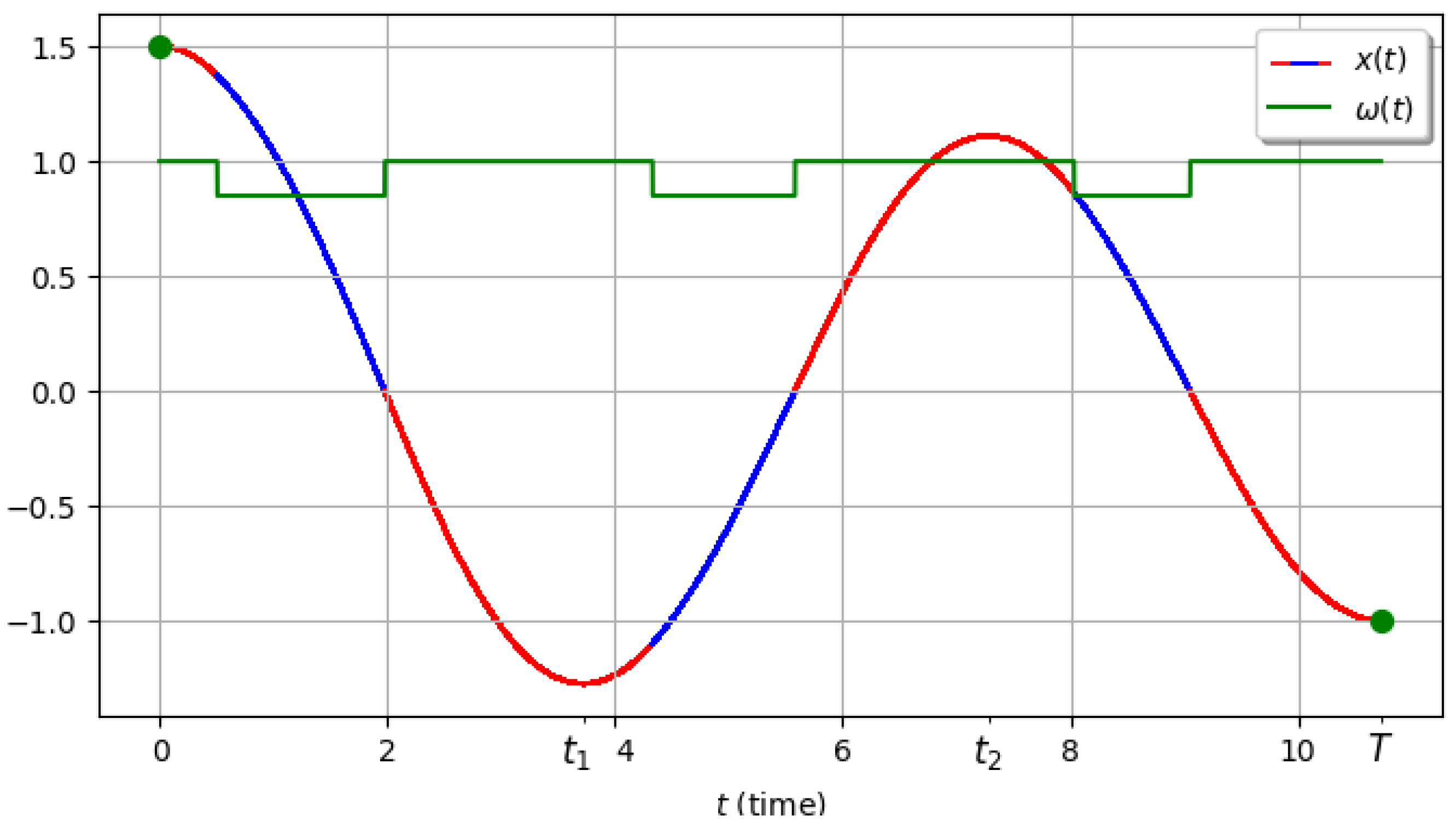
In the last example we choose , , , . The optimal control and the corresponding optimal trajectory are shown in Figure 14. In this case, for relatively large values of the variable x, the optimal control strongly deviates from periodic behavior. There is a noticeable difference in the duration of individual semi-oscillations.
9. Conclusions
In this work, we solved the minimum-time optimal control problem for a nonlinear pendulum-type oscillator, where the control parameter is its natural frequency constrained to the interval . The objective was to transfer the system from one arbitrary rest state to another in the shortest possible time.
By applying Pontryagin’s maximum principle and Bellman’s principle of optimality, we decomposed the original problem into a sequence of similar subproblems corresponding to single semi-oscillations. For each such subproblem, it was rigorously shown that the optimal control is of relay (bang–bang) type and contains no more than two switchings. This, in turn, reduces the dynamics on each semi-oscillation to three segments with constant control.
A key analytical result is the derivation of expressions for the switching times and the total duration of a semi-oscillation in terms of elliptic integrals. This made it possible to reduce the original infinite-dimensional optimal control problem to a finite-dimensional minimization problem, namely the search for an optimal sequence of intermediate semi-oscillation amplitudes. The resulting finite-dimensional problem was solved numerically using dynamic programming, which enabled us to construct the Bellman function (the optimal-time function) and, simultaneously, to recover the optimal control in the original problem.
Numerical examples confirmed the effectiveness of the proposed approach. A particularly important outcome is the demonstration of qualitative differences from the analogous linear problem (where ). In the nonlinear case, the optimal control is generally non-periodic: as the computations show, the duration of semi-oscillations and the control structure (switching type) may vary irregularly with the current amplitude, reflecting the intrinsic nonlinearity of . From a numerical perspective, it is natural to compare the proposed dynamic programming scheme with state-of-the-art direct optimal control and NMPC solvers [29,30,31].
Overall, the paper provides a structurally explicit and computationally efficient solution to the minimum-time frequency control problem for a nonlinear oscillator, combining PMP-based switching analysis with elliptic-integral timing and dynamic programming for multi–semi-oscillation transfers. This work lays a theoretical foundation for further research. The most promising directions include:
- Incorporating dissipative forces into the model, primarily Coulomb and viscous friction, which will complicate the Hamiltonian but bring the model significantly closer to real physical systems.
- Introducing constraints on the rate of change of the control (slew-rate constraints), i.e., , which is more realistic from an engineering point of view.
- Extending the proposed approach to systems with multiple degrees of freedom, such as spherical pendulums or models of robotic manipulators.
Author Contributions
Conceptualization, V.T.; investigation, D.K., V.I., and V.T. All authors have read and agreed to the published version of the manuscript.
Funding
This research received no external funding.
Data Availability Statement
The code that is developed within this paper is available from the corresponding author(s) upon a request.
Conflicts of Interest
The authors declare no conflicts of interest.
Nomenclature
| t | Time variable |
| , | Coordinate function, Velocity, Acceleration |
| Boundary conditions | |
| Control function | |
| , | Lower and upper limits of the control function |
| T | Optimal time |
| , | Control switching points |
| A, B | Boundary conditions for one semi-oscillation |
References
- Pontryagin, L.S. The Mathematical Theory of Optimal Processes; Routledge: London, UK, 1987. [CrossRef]
- Athans, M.; Falb, P. Optimal Control; McGraw–Hill: New York, NY, USA, 1966.
- Bryson, A.E.; Ho, Y.-C. Applied Optimal Control; Hemisphere: Washington, DC, USA, 1975. [CrossRef]
- Bellman, R. Dynamic Programming; Princeton University Press: Princeton, NJ, USA, 1957.
- Tang, W.; Ma, R.; Wang, W.; Gao, H. Optimization-Based Input-Shaping Swing Control of Overhead Cranes. Appl. Sci. 2023, 13, 9637. [CrossRef]
- Tang, W.; Zhao, E.; Sun, L.; Gao, H. An Active Swing Suppression Control Scheme of Overhead Cranes Based on Input-Shaping Model Predictive Control. Syst. Sci. Control Eng. 2023, 11, 2188401. [CrossRef]
- Cao, X.-H.; Meng, C.; Zhou, Y.; Zhu, M. An Improved Negative Zero-Vibration Anti-Swing Control Strategy for Grab Ship Unloader based on elastic wire rope model. Mech. Ind. 2021, 22, 45. [CrossRef]
- Wu, Q.; Wang, X.; Hua, L.; Xia, M. Improved Time-Optimal Anti-Swing Control for Double-Pendulum Systems. Mech. Syst. Signal Process. 2021, 151, 107444. [CrossRef]
- Huang, W.; Niu, W.; Zhou, X.; Gu, W. Anti-Sway Control of Variable Rope-Length Container Crane Based on Phase Plane Trajectory Planning. J. Vib. Control 2024, 30, 1227–1240. [CrossRef]
- Ouyang, H.; Tian, Z.; Yu, L.; Zhang, G. Motion Planning for Payload Swing Suppression in Tower Cranes. J. Frankl. Inst. 2020, 357, 8299–8320. [CrossRef]
- Li, G.; Ma, X.; Li, Z.; Li, Y. Optimal Trajectory Planning for Double-Pendulum Tower Cranes. IEEE/ASME Trans. Mechatron. 2023, 28, 919–932. [CrossRef]
- Tian, D.; Liu, Z. Period/Frequency Estimation of Nonlinear Oscillators. J. Low Freq. Noise Vib. Act. Control 2019. [CrossRef]
- He, C.-H. A Complement to Nonlinear Oscillator Frequency Estimation. J. Low Freq. Noise Vib. Act. Control 2019. [CrossRef]
- Zhang, L.; Gepreel, K.; Yu, J. He’s Frequency Formulation for Fractal–Fractional Nonlinear Oscillators. Front. Phys. 2025, 13, 1542758. [CrossRef]
- Liu, C.; Zhou, T.; Gong, Z.; Yi, X.; Teo, K.L.; Wang, S. Robust Optimal Control of Fractional Nonlinear Systems. Chaos Solitons Fractals 2023, 175, 113964. [CrossRef]
- He, J.-H. Variational Iteration Method–A Kind of Non-Linear Analytical Technique: Some Examples. Int. J. Nonlin. Mech. 1999, 34, 699–708. [CrossRef]
- Wei, Q.; Liu, D.; Lin, H. Value Iteration Adaptive Dynamic Programming for Optimal Control of Discrete-Time Nonlinear Systems. IEEE Trans. Cybern. 2016, 46, 840–853. [CrossRef]
- Wei, Q.; Li, T. Constrained Adaptive Dynamic Programming. IEEE Trans. Neural Netw. Learn. Syst. 2024, 35, 3251–3264. [CrossRef]
- Wang, J.; Zhang, P.; Wang, Y.; Ji, Z. Adaptive Dynamic Programming for Nonlinear Systems with Input Delay. Nonlinear Dyn. 2023, 111, 19133–19149. [CrossRef]
- Lewis, F.L.; Vrabie, D.; Syrmos, V. Optimal Control and Reinforcement Learning; Wiley: Hoboken, NJ, USA, 2012. [CrossRef]
- Bertsekas, D. Dynamic Programming and Optimal Control, 4th ed.; Athena Scientific: Belmont, MA, USA, 2017.
- Gao, S.; Liu, E.; Wu, Z.; Li, J.; Zhang, M. Neural ODE-Based Frequency Stability Assessment and Control of Energy Storage Systems. Appl. Sci. 2025, 15, 12048. [CrossRef]
- Shah, A.A.; Han, X.; Armghan, H.; Almani, A.A. A Nonlinear Integral Backstepping Controller to Regulate the Voltage and Frequency of an Islanded Microgrid Inverter. Electronics 2021, 10, 660. [CrossRef]
- Meng, D.; Lu, W.; Xu, W.; She, Y.; Wang, X.; Liang, B.; Yuan, B. Vibration Suppression Control of Free-Floating Space Robots with Flexible Appendages for Autonomous Target Capturing. Acta Astronaut. 2018, 151, 904–918. [CrossRef]
- Kamzolkin, D.; Ilyutko, V.; Ternovski, V. Optimal Control of a Harmonic Oscillator with Parametric Excitation. Mathematics 2024, 12, 3981. [CrossRef]
- Kamzolkin, D.; Ternovski, V. Time-Optimal Motions of Systems with Viscous Friction. Mathematics 2024, 12, 1485. [CrossRef]
- Diaz, J.B.; McLaughlin, J.R. Sturm comparison theorems for ordinary and partial differential equations. Bulletin of the American Mathematical Society, Bull. Amer. Math. Soc. 75(2), 335-339, (March 1969).
- Abramowitz, M.; Stegun, I.A., Eds. Handbook of Mathematical Functions with Formulas, Graphs, and Mathematical Tables; National Bureau of Standards: Washington, DC, USA, 1964.
- Betts, J.T. Practical Methods for Optimal Control and Estimation Using Nonlinear Programming, 2nd ed.; SIAM: Philadelphia, PA, USA, 2010. [CrossRef]
- Ross, I.M.; Fahroo, F. Pseudospectral Knotting Methods for Solving Optimal Control Problems. J. Guid. Control Dyn. 2004, 27, 397–405. [CrossRef]
- Diehl, M.; Ferreau, H.J.; Haverbeke, N. Efficient Numerical Methods for Nonlinear MPC and Moving Horizon Estimation. In Nonlinear Model Predictive Control; Findeisen, R., Allgöwer, F., Biegler, L.T., Eds.; Springer: Berlin/Heidelberg, Germany, 2009; pp. 391–417. [CrossRef]
Figure 1.
Hypothetical solution to the equations (14), representing the zeros of functions and (red dots). (We have proved that such an arrangement of zeros of the two functions is impossible).
Figure 1.
Hypothetical solution to the equations (14), representing the zeros of functions and (red dots). (We have proved that such an arrangement of zeros of the two functions is impossible).
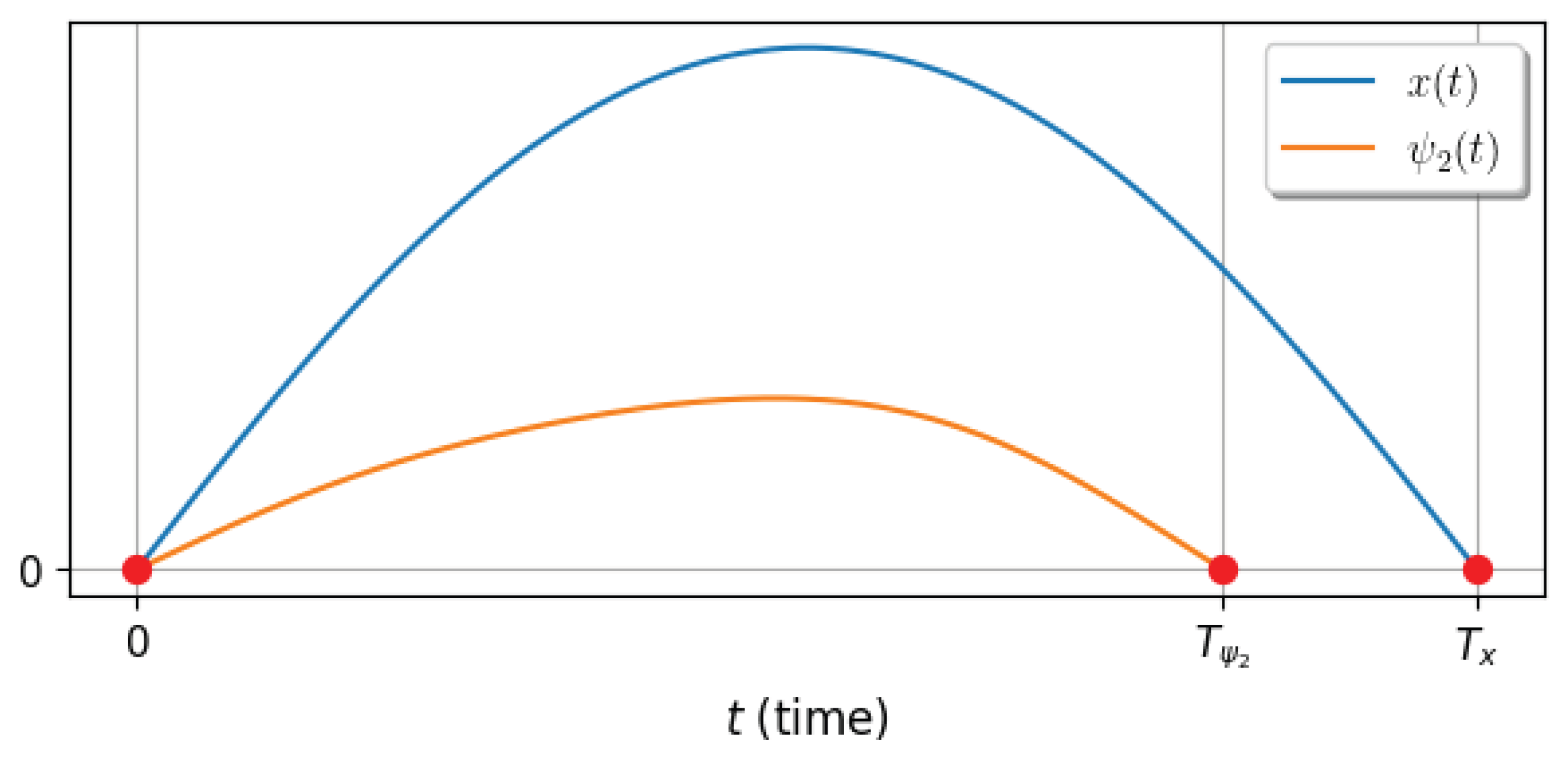
Figure 2.
Distances between zeros of the functions and as functions of the parameter .
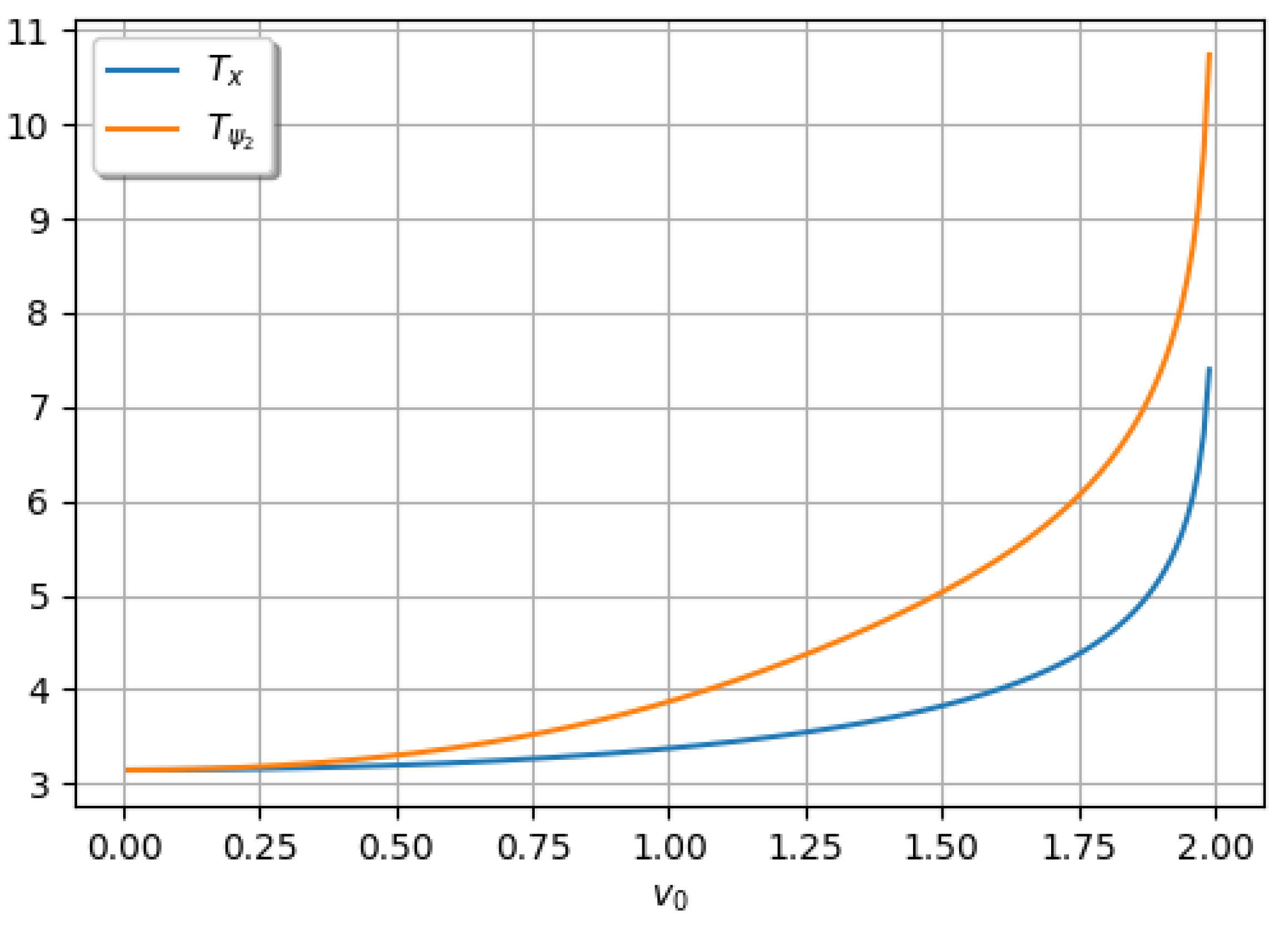
Figure 3.
(1)-(5) – all possible variants of optimal control encountered in problem (5). Here .
Figure 3.
(1)-(5) – all possible variants of optimal control encountered in problem (5). Here .
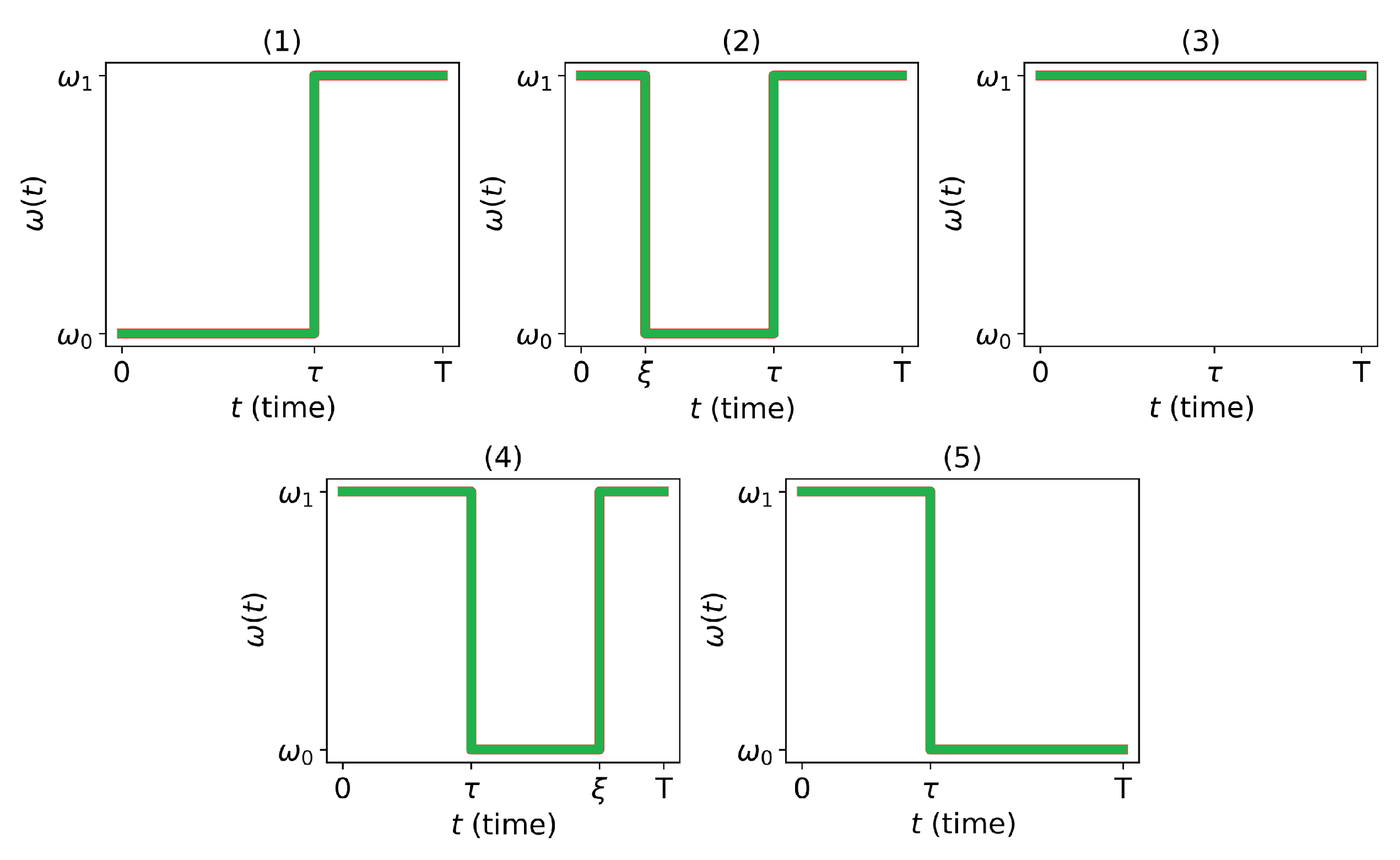
Figure 4.
(1)-(3) – nonoptimal control types encountered while applying PMP to problem (5). Here .
Figure 4.
(1)-(3) – nonoptimal control types encountered while applying PMP to problem (5). Here .
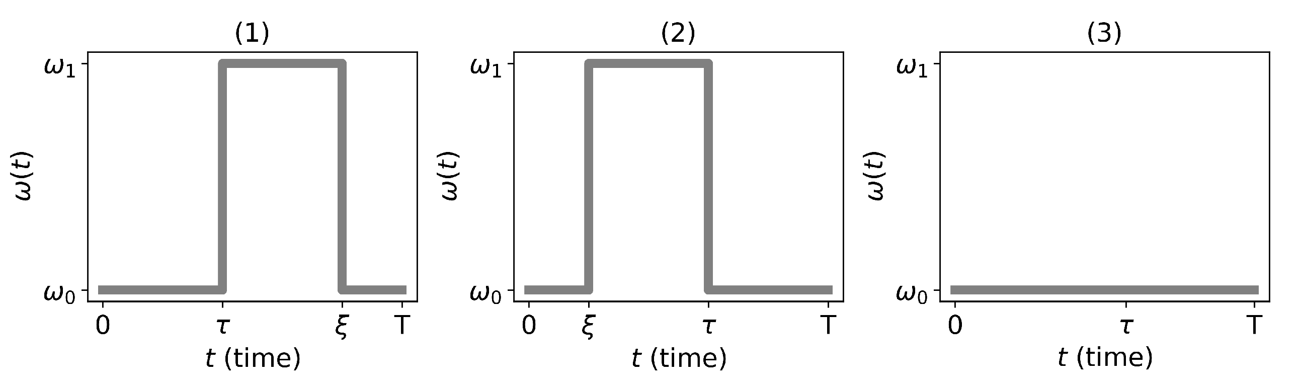
Figure 5.
Plot of the function Here, and the number of semi-oscillations is one.
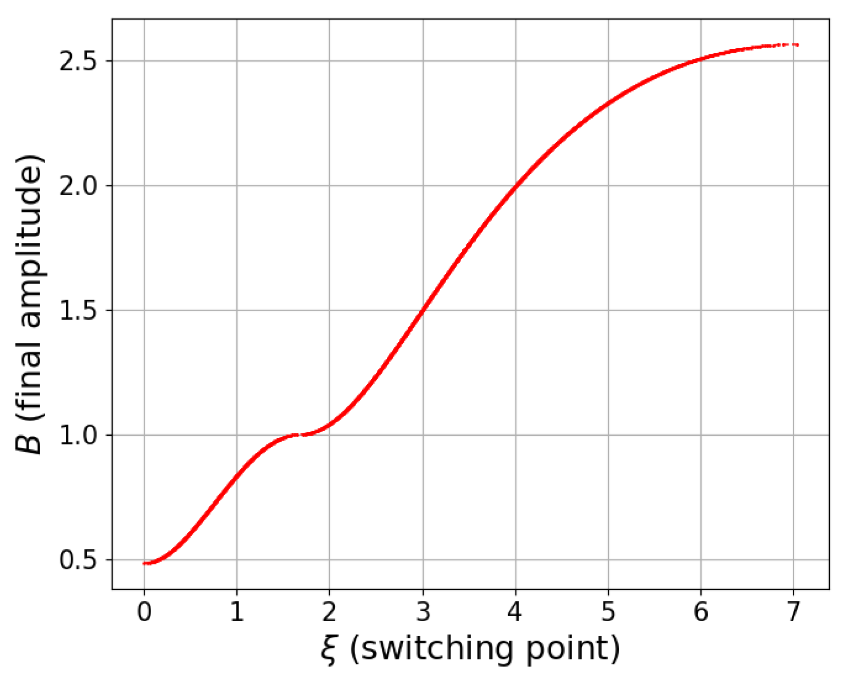
Figure 6.
Domains of values A and B (aquamarine color) for which problem (5) has a solution. (a), , (b), , (c), .
Figure 6.
Domains of values A and B (aquamarine color) for which problem (5) has a solution. (a), , (b), , (c), .
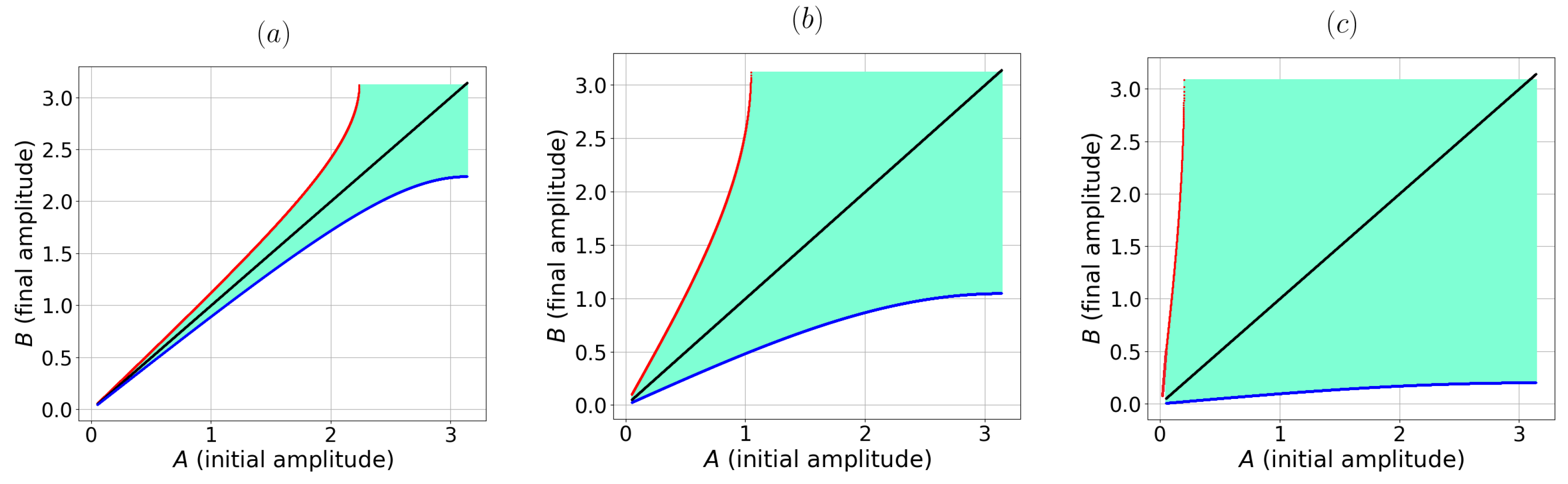
Figure 7.
Plot of optimal process time of one semi-oscillation versus initial and final amplitudes. Here , .
Figure 7.
Plot of optimal process time of one semi-oscillation versus initial and final amplitudes. Here , .
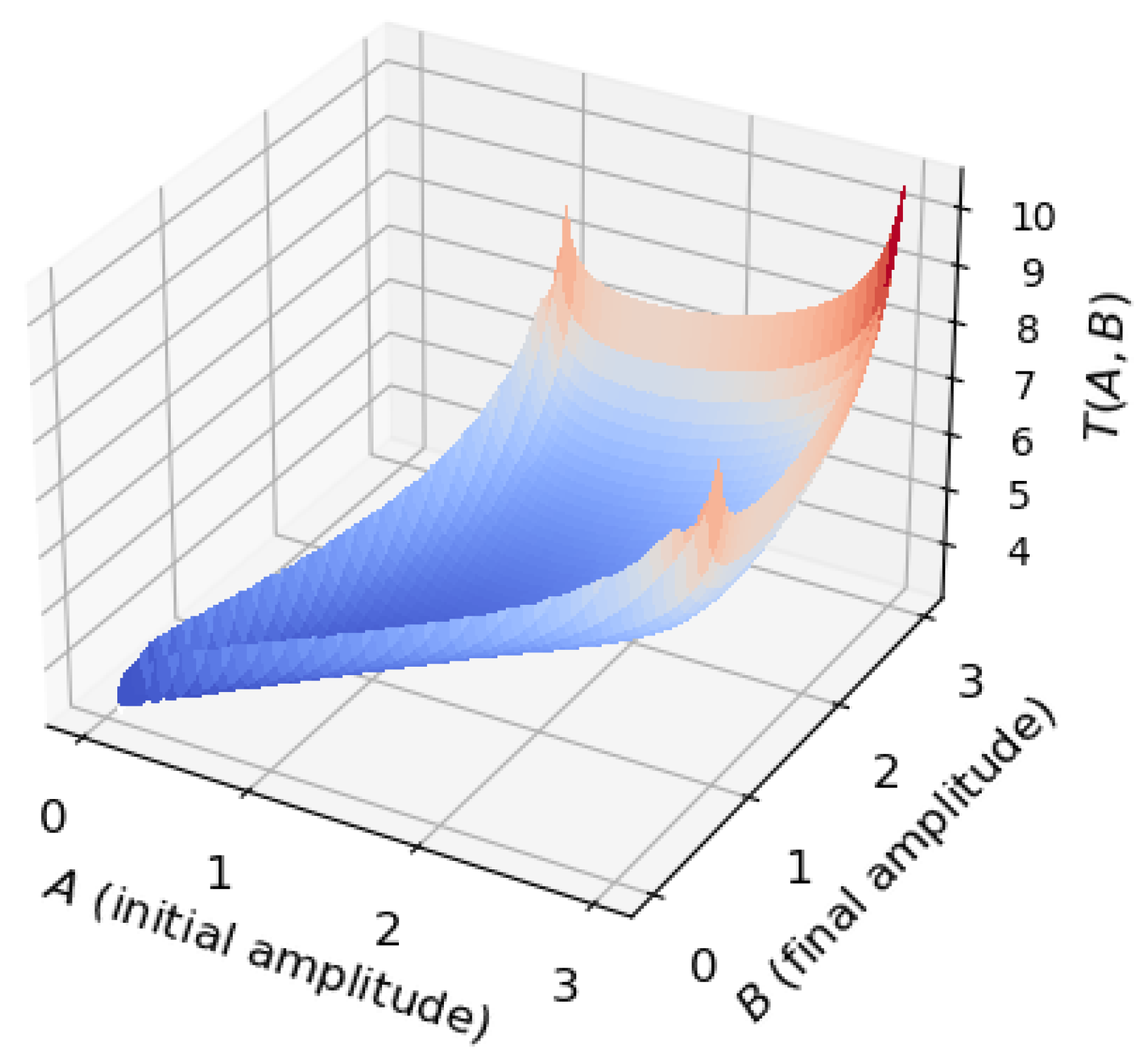
Figure 8.
Decomposition of the trajectory of the controlled system (4) into n semi-oscillations.
Figure 8.
Decomposition of the trajectory of the controlled system (4) into n semi-oscillations.
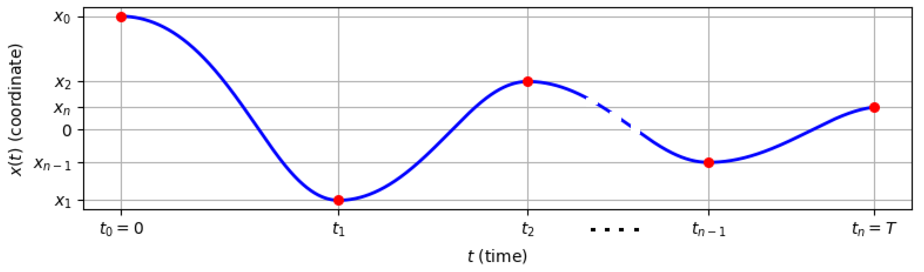
Figure 9.
Plot of the optimal time T in problem (4) versus the terminal state . Here, , , , and the number of semi-oscillations is at most 10.
Figure 9.
Plot of the optimal time T in problem (4) versus the terminal state . Here, , , , and the number of semi-oscillations is at most 10.
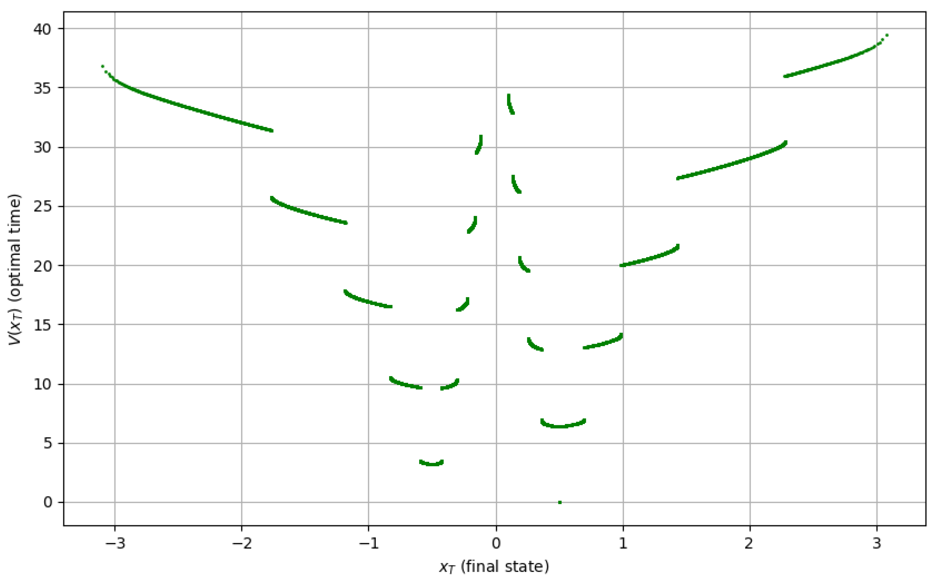
Figure 10.
Family of optimal trajectories starting from the given initial point . The case of all possible terminal states reachable in no more than three semi-oscillations. Here , . Red corresponds to the control value , blue to the control value . Green dots indicate the initial and various terminal states.
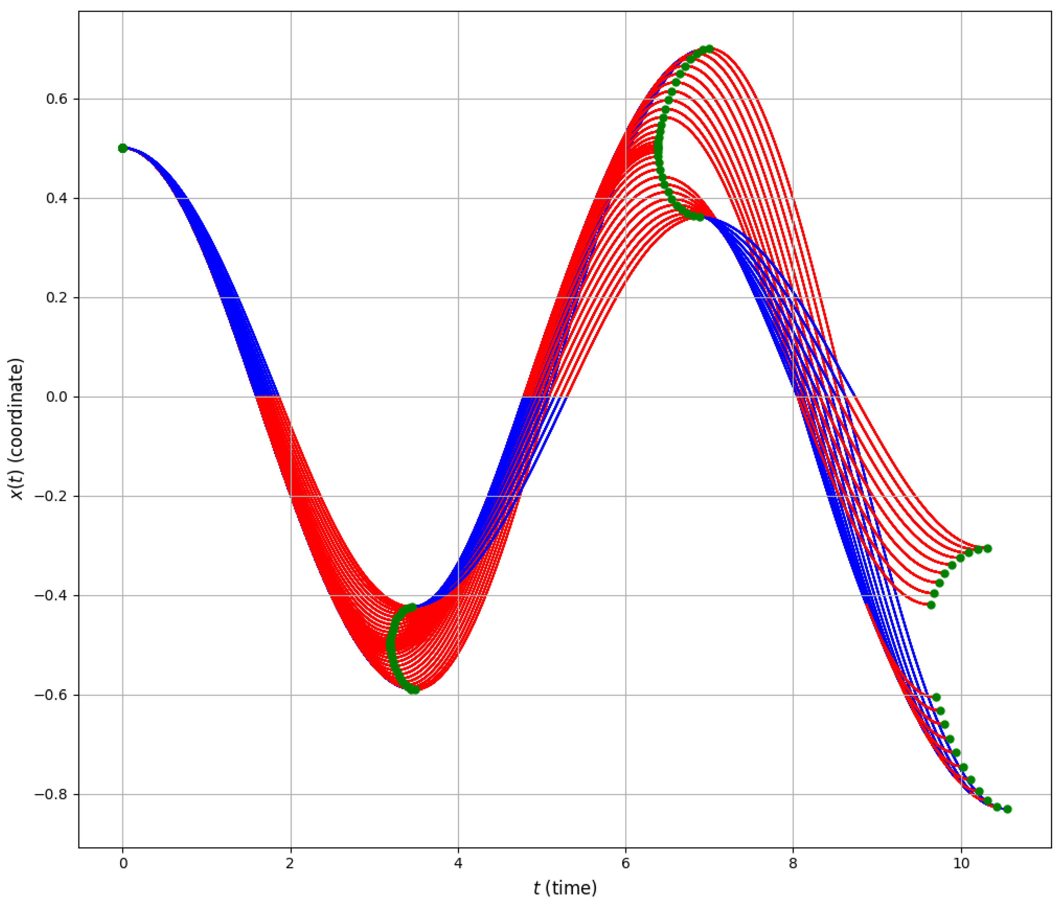
Figure 11.
Phase portrait of optimal trajectories starting from the given initial point . The case of all possible terminal states reachable in no more than three semi-oscillations. Here , . Red corresponds to the control value , blue to the control value . Green dots indicate the initial and various terminal states.
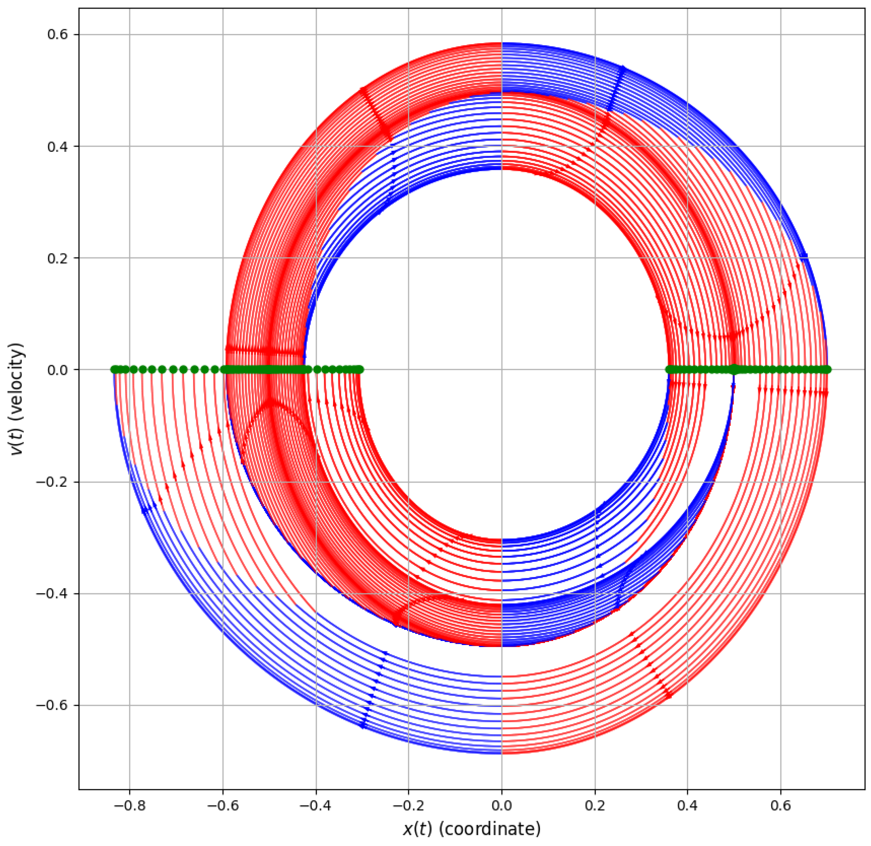
Figure 12.
Plots of the optimal trajectory and the optimal control. Here , , , , , and the number of semi-oscillations is 2. For such close initial and terminal conditions, one can obtain different types of control on the semi-oscillations, which is not typical for the linear case.
Figure 12.
Plots of the optimal trajectory and the optimal control. Here , , , , , and the number of semi-oscillations is 2. For such close initial and terminal conditions, one can obtain different types of control on the semi-oscillations, which is not typical for the linear case.
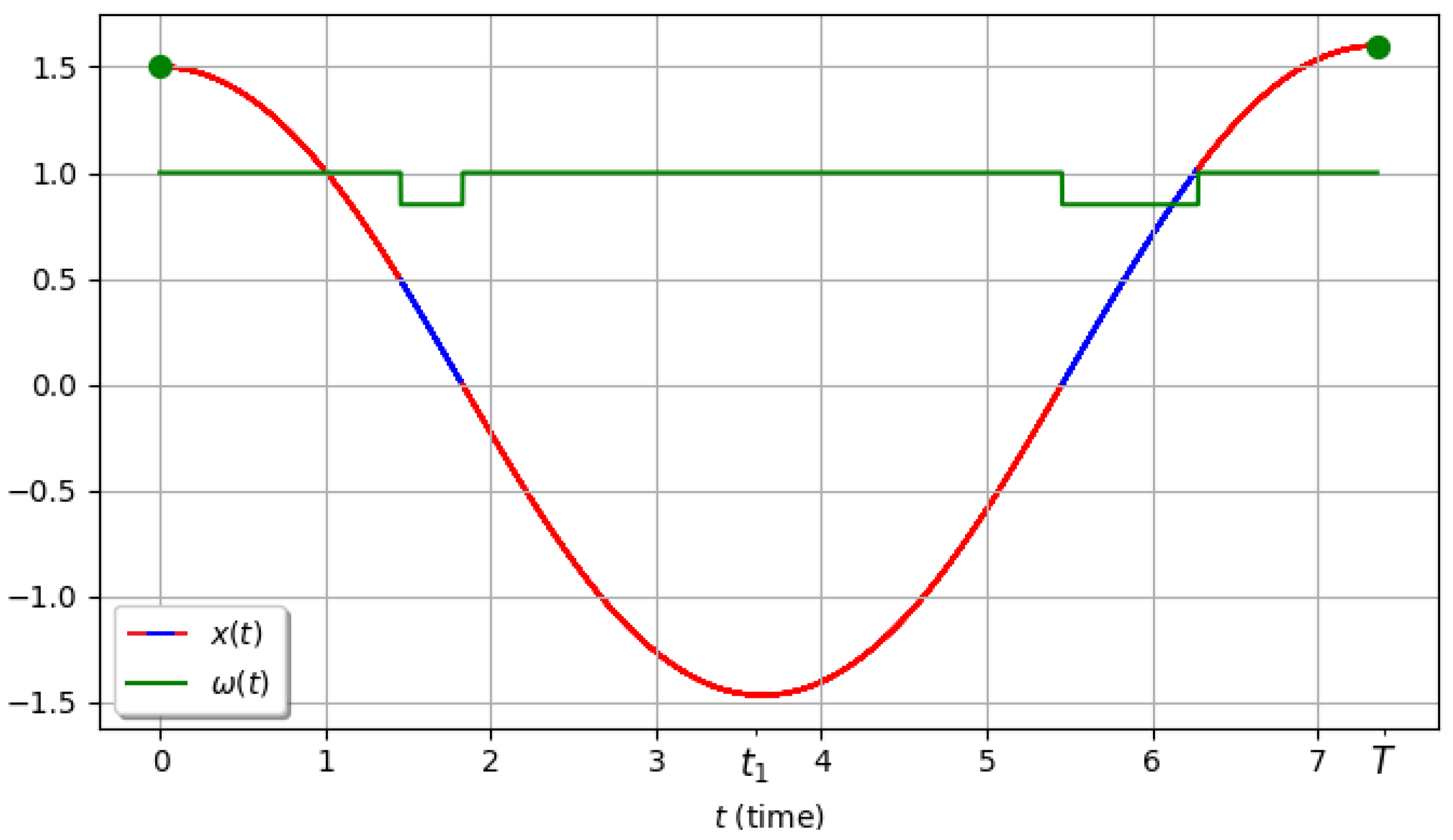
Figure 13.
Plots of the optimal trajectory and the optimal control. Here , , , , , and the number of semi-oscillations is 3. For small values of the variable x, the optimal control is close to periodic: , , .
Figure 13.
Plots of the optimal trajectory and the optimal control. Here , , , , , and the number of semi-oscillations is 3. For small values of the variable x, the optimal control is close to periodic: , , .
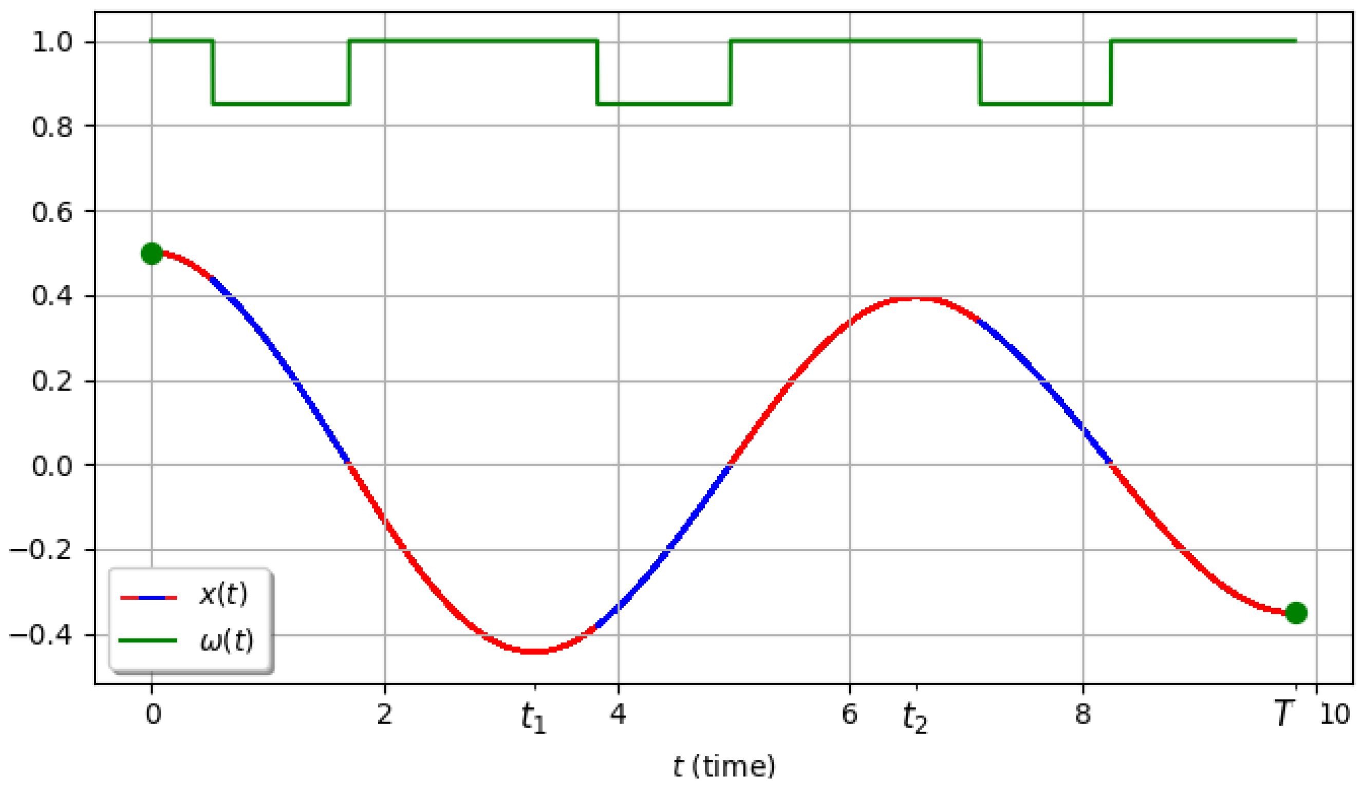
Figure 14.
Plots of the optimal trajectory and the optimal control. Here , , , , , and the number of semi-oscillations is 3. For large values of the variable x, the dynamics of the nonlinear system differ from the linear case, and the optimal control is far from periodic: , , .
Figure 14.
Plots of the optimal trajectory and the optimal control. Here , , , , , and the number of semi-oscillations is 3. For large values of the variable x, the dynamics of the nonlinear system differ from the linear case, and the optimal control is far from periodic: , , .
Disclaimer/Publisher’s Note: The statements, opinions and data contained in all publications are solely those of the individual author(s) and contributor(s) and not of MDPI and/or the editor(s). MDPI and/or the editor(s) disclaim responsibility for any injury to people or property resulting from any ideas, methods, instructions or products referred to in the content. |
© 2025 by the authors. Licensee MDPI, Basel, Switzerland. This article is an open access article distributed under the terms and conditions of the Creative Commons Attribution (CC BY) license (http://creativecommons.org/licenses/by/4.0/).
Copyright: This open access article is published under a Creative Commons CC BY 4.0 license, which permit the free download, distribution, and reuse, provided that the author and preprint are cited in any reuse.


