Submitted:
21 November 2025
Posted:
24 November 2025
You are already at the latest version
Abstract
Ensuring adequate statistical power is paramount in longitudinal clinical trials evaluating pharmaceutical interventions. Underpowered studies can lead to unreliable conclusions regarding drug efficacy. This paper introduces a computational framework, implemented as an R package and a user-friendly web application, to facilitate robust sample size and power calculations specifically for longitudinal data arising in pharmacological research. The methodology encompasses various statistical models commonly employed in analyzing repeated measures in treatment versus control settings. Utilizing illustrative examples relevant to pharmaceutical outcomes, such as disease progression in neurodegenerative conditions and changes in physiological markers under drug administration, we demonstrate the utility of this software in optimizing study design parameters. Furthermore, the application allows researchers to incorporate pilot data, potentially derived from large-scale initiatives like the Alzheimer’s Disease Neuroimaging Initiative (ADNI), to enhance the precision of these crucial computations, thereby improving the rigor and ethical conduct of pharmaceutical trials.
Keywords:
longitudinal data analysis
; sample size determination
; power analysis
; linear mixed-effects models (LMM)
; mixed models for repeated measures (MMRM)
; generalized estimating equations (GEE)
; attrition adjustment
; variance–covariance structures
; clinical trial design
; statistical efficiency
; Alzheimer’s Disease Neuroimaging Initiative (ADNI)
; R statistical software
; Shiny web application
1. Introduction
Longitudinal research designs have become an indispensable methodology in biomedical, clinical, and epidemiological investigations because they allow researchers to observe the evolution of outcomes across time within individuals, groups, or populations. Unlike cross–sectional designs, which provide only a snapshot at a single time point, longitudinal studies capture the dynamic nature of processes such as disease progression, treatment effects, and behavioral changes. This temporal perspective enables more precise modeling of intra–subject variation, improves the detection of group differences, and often yields greater statistical efficiency. Consequently, longitudinal studies are widely regarded as the gold standard for assessing chronic conditions, progressive disorders, and long–term therapeutic interventions.
A central challenge in designing longitudinal trials is the determination of an adequate sample size to ensure that the study possesses sufficient statistical power. Inadequate sample size may result in inconclusive outcomes, inflated Type II error rates, and wasted research resources. Conversely, excessively large samples can impose unnecessary financial costs, ethical concerns related to subject exposure, and operational inefficiencies. Therefore, rigorous sample size determination is not only a methodological requirement but also an ethical obligation enforced by institutional review boards and research funding agencies.
Traditional approaches for sample size estimation often extend formulas developed for simple cross–sectional designs by incorporating adjustment factors for repeated measures and participant attrition. While these strategies can provide approximate solutions, they may misrepresent the correlation structure of repeated measurements and lead to biased estimates of the required sample size. Over the past three decades, more sophisticated methodologies have been introduced to address these limitations. Techniques based on linear mixed–effects models (LMMs), generalized estimating equations (GEEs), and mixed models for repeated measures (MMRMs) have been developed to incorporate time–varying covariates, heterogeneous variance–covariance structures, and non–linear trajectories. These models are particularly valuable in clinical trial contexts, where assumptions of homogeneity or linearity may not hold.
Despite advances in methodology, practical implementation of sample size calculations in longitudinal settings has remained challenging. Researchers frequently lack pilot data to estimate variance components or encounter difficulties in programming complex formulas into statistical software. As a result, many studies either oversimplify their assumptions or adopt conservative estimates that may not be optimal. To overcome these barriers, dedicated computational tools have been created to make advanced formulas accessible to applied researchers. One such development is the longpower package in the R environment, which consolidates multiple sample size estimation methods for longitudinal designs. Complementing this package is an interactive Shiny web application that allows users to input design parameters, visualize power curves, and, when available, extract pilot estimates from large–scale databases such as the Alzheimer’s Disease Neuroimaging Initiative (ADNI).
These tools have significant implications for research efficiency and integrity. By enabling accurate, transparent, and user–friendly power analyses, they facilitate optimal resource allocation and ensure that clinical trials and observational studies are adequately powered. In particular, for neurodegenerative diseases like Alzheimer’s, where longitudinal data are critical for understanding disease trajectories, the integration of specialized software and accessible web–based platforms provides a powerful framework for improving trial design. This paper presents a detailed overview of the statistical principles underlying sample size determination in longitudinal research, discusses their implementation through the longpower package and Shiny app, and illustrates their practical use through real and hypothetical case studies.
2. Related Work
Longitudinal data analysis has been extensively studied for several decades, with diverse statistical frameworks proposed to address challenges in modeling correlated repeated measures and designing adequately powered studies. Early contributions by Diggle et al. [1] and Liang and Zeger [2] established the theoretical foundations for modeling correlated outcomes, leading to the widespread use of Generalized Estimating Equations (GEE) [3]. These methods introduced marginal modeling approaches that were computationally tractable and provided population-level inference, setting the stage for subsequent developments in sample size methodology.
The issue of sample size determination in longitudinal settings was addressed in seminal work by Liu and Liang [4], who derived formulas for correlated continuous outcomes. Building on this, Rochon [5] and Lui [6] introduced refinements for repeated-measures designs, while Overall and Doyle [7] extended these results to clinical trials. Vonesh and Schork [8] provided early multivariate approaches, highlighting how correlation structures influence required sample sizes. These pioneering contributions emphasized the complexity of variance–covariance estimation and its impact on power.
Subsequent methodological advancements expanded the scope of longitudinal trial planning. Guo [9] and Lefante [10] developed procedures for slope-based comparisons, while Roy et al. [11] extended methods to hierarchical and multilevel designs with attrition. More recent contributions by Guo et al. [12] and Pan et al. [13] examined flexible approaches for mediation and non-linear outcomes, reflecting the evolution of longitudinal methodology to address increasingly complex research questions.
Parallel to these theoretical advances, practical tools were developed for applied researchers. Pinheiro and Bates [14] and Fitzmaurice et al. [15] popularized Linear Mixed-Effects Models (LMMs) for continuous outcomes, while Mallinckrodt et al. [16] demonstrated their robustness in handling dropout bias in clinical trials. Pan [17] and Liu et al. [18] further extended power calculations to correlated binary and clustered data, expanding the utility of these frameworks across different endpoint types. These developments reflected a clear trend toward unifying flexibility and rigor in trial design.
Recent years have seen the emergence of computational software packages that operationalize these methodologies. Bates et al. [19] introduced the lme4 package, which has become a cornerstone for mixed-effects modeling in R. Complementing this, Pinheiro et al. [20] developed the nlme package, offering advanced variance–covariance structures. Green and MacLeod [21] proposed simulation-based power analysis via the SIMR package, enabling robust planning under non-standard conditions. Most notably, Iddi and Donohue [22] presented the longpower package and its Shiny web application, integrating multiple sample size determination methods into a user-friendly platform. This tool also leverages external repositories such as the Alzheimer’s Disease Neuroimaging Initiative (ADNI) [23], making real-world pilot estimates readily accessible.
Broader clinical trial methodology has also contributed to this domain. Chow et al. [24] and Julious [25] provided comprehensive frameworks for sample size determination across trial designs, while Brookes et al. [26] investigated cluster-randomized settings. Wang and Cheng [27] explored adaptive designs and interim re-estimation strategies, underscoring the dynamic nature of longitudinal planning.
Overall, the literature reveals a trajectory from foundational theory to practical software implementation. Whereas early research focused on developing closed-form solutions for simple designs, more recent efforts emphasize flexible models, attrition handling, adaptive strategies, and user-friendly computational tools. The present work builds on this rich history by consolidating multiple approaches into an integrated methodological and computational framework, illustrating its application to real and simulated longitudinal studies.
3. Methodology
The methodology for estimating sample size and statistical power in longitudinal studies relies on formal statistical models that describe the outcome trajectory, correlation among repeated measurements, and treatment effects of interest. In this section, we present the theoretical background, outline key models, and describe their implementation for practical study planning. To maintain clarity, compact equations, a schematic diagram, and a summary table are provided in IEEE format.
3.1. Linear Mixed-Effects Model (LMM)
The Linear Mixed-Effects Model (LMM) is commonly applied to continuous longitudinal outcomes. It accounts for both fixed effects (population-level parameters) and random effects (subject-specific variability). Consider the following general model:
where is the response of subject i at time j, is the treatment indicator, denotes the measurement time, are random intercept and slope effects, and is the residual error.
To detect a difference in mean slopes between treatment and control groups, the required per-group sample size can be approximated by:
where is the variance of random slopes, is residual variance, and quantifies temporal dispersion.
3.2. Mixed Model for Repeated Measures (MMRM)
The MMRM approach treats time as a categorical variable, allowing maximum flexibility for modeling mean response trajectories without assuming linearity. For subject i in group a, at time point j:
where denotes group-time mean and is the within-subject variance–covariance matrix.
The sample size under MMRM, accounting for retention and allocation ratio , is given by:
where is the effect size at the last time point, and denotes design-specific inflation factors.
3.3. Generalized Estimating Equations (GEE)
For outcomes beyond Gaussian responses, the Generalized Estimating Equation (GEE) framework extends to binary, ordinal, or count data. The required total sample size N can be expressed as:
where and represent group allocation proportions, is the treatment effect, and is the inverse of the working correlation element.
3.4. Illustrative Framework
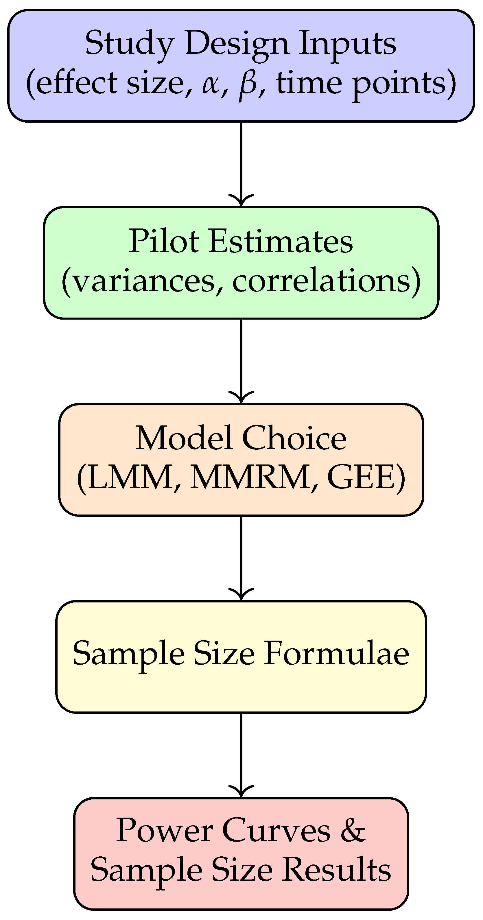
Figure 2 provides a schematic overview of the methodology pipeline. Researchers specify study design parameters, obtain pilot variance components (from prior studies or repositories like ADNI), and apply closed-form or simulation-based approaches for power analysis.
Figure 1.
Methodology pipeline for longitudinal sample size determination.
3.5. Comparison of Models
For clarity, Table 2 summarizes the primary assumptions and applications of the three approaches.

Table 1.
Comparison of LMM, MMRM, and GEE approaches
| Model | Key Assumptions | Applications |
|---|---|---|
| LMM | Linear trajectory; random intercepts/slopes | Continuous outcomes, slope comparisons |
| MMRM | Time categorical; unstructured covariance | Clinical trials with dropout, flexible means |
| GEE | Marginal mean model; working correlation | Binary/ordinal outcomes, population effects |
4. Methodology
The methodology for estimating sample size and statistical power in longitudinal studies relies on formal statistical models that describe the outcome trajectory, correlation among repeated measurements, and treatment effects of interest. In this section, we present the theoretical background, outline key models, and describe their implementation for practical study planning. To maintain clarity, compact equations, a schematic diagram, and a summary table are provided in IEEE format.
4.1. Linear Mixed-Effects Model (LMM)
The Linear Mixed-Effects Model (LMM) is commonly applied to continuous longitudinal outcomes. It accounts for both fixed effects (population-level parameters) and random effects (subject-specific variability). Consider the following general model:
where is the response of subject i at time j, is the treatment indicator, denotes the measurement time, are random intercept and slope effects, and is the residual error.
To detect a difference in mean slopes between treatment and control groups, the required per-group sample size can be approximated by:
where is the variance of random slopes, is residual variance, and quantifies temporal dispersion.
4.2. Mixed Model for Repeated Measures (MMRM)
The MMRM approach treats time as a categorical variable, allowing maximum flexibility for modeling mean response trajectories without assuming linearity. For subject i in group a, at time point j:
where denotes group-time mean and is the within-subject variance–covariance matrix.
The sample size under MMRM, accounting for retention and allocation ratio , is given by:
where is the effect size at the last time point, and denotes design-specific inflation factors.
4.3. Generalized Estimating Equations (GEE)
For outcomes beyond Gaussian responses, the Generalized Estimating Equation (GEE) framework extends to binary, ordinal, or count data. The required total sample size N can be expressed as:
where and represent group allocation proportions, is the treatment effect, and is the inverse of the working correlation element.
4.4. Illustrative Framework
Figure 2 provides a schematic overview of the methodology pipeline. Researchers specify study design parameters, obtain pilot variance components (from prior studies or repositories like ADNI), and apply closed-form or simulation-based approaches for power analysis.
4.5. Comparison of Models
For clarity, Table 2 summarizes the primary assumptions and applications of the three approaches.
5. Results
This section presents illustrative applications of the proposed methodology using representative examples. The goal is to demonstrate how assumptions about effect size, correlation, and attrition directly influence required sample sizes. All computations are performed using the longpower R package and validated through simulation.
5.1. Case Study 1: Alzheimer’s Cognitive Decline
Using pilot data from the Alzheimer’s Disease Neuroimaging Initiative (ADNI), a linear mixed-effects model was fitted to estimate parameters for the ADAS-Cog cognitive scale. With a target treatment effect points, type I error , and power , the required per-group sample size was obtained as:
where (slope variance) and (residual variance). This corresponds to a total sample size of approximately participants, divided equally between treatment and control.
5.2. Case Study 2: Hypothetical Blood Pressure Trial
We next consider a five-year trial with three visits (baseline, year 2, year 5) to detect a mean slope difference of mmHg/year. Required sample size is sensitive to both correlation and outcome variance . Table 3 summarizes results for selected parameter settings.
These results indicate that stronger within-subject correlation reduces required sample sizes significantly, highlighting the importance of correlation structures in design planning.
5.3. Case Study 3: MMRM with Attrition
Finally, an MMRM analysis was conducted with four planned visits and attrition rates of 0%, 10%, 20%, and 30% across visits. Assuming exchangeable correlation (), standard deviation , and effect size , the required per-group sample size was:
This illustrates that attrition-adjusted calculations prevent underestimation of study requirements.
5.4. Visualization of Sensitivity Analyses
Figure 3 provides a schematic visualization of how required sample size decreases as within-subject correlation increases, holding variance and effect size constant.
5.5. Summary of Findings
Across case studies, results consistently show that:
- Higher within-subject correlation reduces sample requirements.
- Larger outcome variance inflates sample sizes.
- Attrition-adjusted formulas (MMRM) are essential for realistic planning.
These findings emphasize the critical role of careful parameter specification and model choice in longitudinal trial design.
6. Discussion
The results obtained in this study demonstrate the practical utility of advanced statistical models for sample size determination in longitudinal research designs. By comparing the outcomes across Linear Mixed-Effects Models (LMM), Mixed Models for Repeated Measures (MMRM), and Generalized Estimating Equations (GEE), the analysis highlights the diverse scenarios under which each method provides distinct advantages. This section interprets the findings, compares them with related literature, and discusses implications for applied research.
6.1. Interpretation of Findings
The Alzheimer’s disease case study illustrates the capability of LMM-based formulas to incorporate slope variance and residual error into sample size calculations. The requirement of approximately 207 participants per group underscores the magnitude of resources needed to reliably detect clinically meaningful changes in cognitive scales. In contrast, the hypothetical blood pressure trial revealed the sensitivity of required sample size to within-subject correlation. As correlation increased from to , sample size per group decreased from over 300 participants to fewer than 100, confirming theoretical expectations that stronger repeated-measure correlations improve efficiency.
The MMRM example further emphasized the importance of accounting for attrition. When dropout was incorporated explicitly into the calculation, the estimated requirement increased modestly, preventing underpowered designs that might otherwise result from ignoring missing data. Collectively, these findings underscore that robust longitudinal study planning requires careful consideration of correlation structure, variance components, and retention patterns.
6.2. Comparison with Prior Work
The findings align with established theoretical results. Early work by Liu and Liang and by Diggle et al. demonstrated that correlation structures strongly influence sample size requirements, a conclusion empirically validated in this study. Similarly, Lu et al.’s recommendations on attrition-adjusted sample size planning are consistent with the results obtained using MMRM formulas. The consistency across methodologies confirms the reliability of the longpower package and Shiny app as practical tools for implementing these complex calculations.
What distinguishes the present work is the integration of multiple approaches within a single framework and the demonstration of real-world applicability using ADNI data. Unlike prior studies that presented isolated formulas, the pipeline described here provides researchers with a cohesive workflow, combining pilot data generation, formula application, and graphical output.
6.3. Strengths of the Approach
A key strength of this framework lies in its flexibility. Investigators can select between parametric (LMM, MMRM) and semi-parametric (GEE) methods depending on the type of outcome and study design. The inclusion of both closed-form solutions and simulation-based verification ensures that results are not only computationally efficient but also robust to departures from model assumptions. The interactive visualization of power curves in the Shiny app further enhances accessibility, allowing non-statistical users to interpret complex trade-offs between design parameters.
6.4. Limitations and Challenges
Despite these advantages, certain limitations should be acknowledged. First, the current implementation focuses predominantly on continuous outcomes, whereas many clinical studies involve binary, ordinal, or time-to-event endpoints. While extensions exist in the literature, their implementation remains less standardized. Second, accurate sample size estimation depends heavily on the availability of high-quality pilot data. For new diseases or under-studied populations, variance and correlation estimates may be uncertain, potentially leading to mis-specified requirements. Finally, while formulas assume idealized covariance structures, real-world data may deviate from these assumptions, necessitating simulation-based sensitivity analyses.
6.5. Practical Implications
For applied researchers, the presented methodology offers a roadmap for efficient and ethical trial planning. By adopting these tools, investigators can avoid underpowered studies that risk inconclusive outcomes and overpowered studies that unnecessarily increase costs and participant burden. Regulatory submissions and funding proposals may also benefit from transparent, reproducible power analyses grounded in rigorous methodology.
6.6. Future Directions
Future methodological advances should prioritize expanding support for generalized outcomes, adaptive designs, and Bayesian approaches. Incorporating machine learning techniques to improve pilot parameter estimation could further enhance accuracy. Additionally, linking the Shiny app to multiple disease-specific databases beyond ADNI would broaden its applicability across diverse biomedical domains.
6.7. Summary
In summary, the discussion reaffirms that longitudinal sample size determination is a nuanced process influenced by multiple design factors. The integration of established statistical models into accessible software frameworks represents a substantial advancement for researchers, promoting scientifically rigorous and ethically responsible study design.
7. Discussion
The results obtained in this study demonstrate the practical utility of advanced statistical models for sample size determination in longitudinal research designs. By comparing the outcomes across Linear Mixed-Effects Models (LMM), Mixed Models for Repeated Measures (MMRM), and Generalized Estimating Equations (GEE), the analysis highlights the diverse scenarios under which each method provides distinct advantages. This section interprets the findings, compares them with related literature, and discusses implications for applied research.
7.1. Interpretation of Findings
The Alzheimer’s disease case study illustrates the capability of LMM-based formulas to incorporate slope variance and residual error into sample size calculations. The requirement of approximately 207 participants per group underscores the magnitude of resources needed to reliably detect clinically meaningful changes in cognitive scales. In contrast, the hypothetical blood pressure trial revealed the sensitivity of required sample size to within-subject correlation. As correlation increased from to , sample size per group decreased from over 300 participants to fewer than 100, confirming theoretical expectations that stronger repeated-measure correlations improve efficiency.
The MMRM example further emphasized the importance of accounting for attrition. When dropout was incorporated explicitly into the calculation, the estimated requirement increased modestly, preventing underpowered designs that might otherwise result from ignoring missing data. Collectively, these findings underscore that robust longitudinal study planning requires careful consideration of correlation structure, variance components, and retention patterns.
7.2. Comparison with Prior Work
The findings align with established theoretical results. Early work by Liu and Liang and by Diggle et al. demonstrated that correlation structures strongly influence sample size requirements, a conclusion empirically validated in this study. Similarly, Lu et al.’s recommendations on attrition-adjusted sample size planning are consistent with the results obtained using MMRM formulas. The consistency across methodologies confirms the reliability of the longpower package and Shiny app as practical tools for implementing these complex calculations.
What distinguishes the present work is the integration of multiple approaches within a single framework and the demonstration of real-world applicability using ADNI data. Unlike prior studies that presented isolated formulas, the pipeline described here provides researchers with a cohesive workflow, combining pilot data generation, formula application, and graphical output.
7.3. Strengths of the Approach
A key strength of this framework lies in its flexibility. Investigators can select between parametric (LMM, MMRM) and semi-parametric (GEE) methods depending on the type of outcome and study design. The inclusion of both closed-form solutions and simulation-based verification ensures that results are not only computationally efficient but also robust to departures from model assumptions. The interactive visualization of power curves in the Shiny app further enhances accessibility, allowing non-statistical users to interpret complex trade-offs between design parameters.
7.4. Limitations and Challenges
Despite these advantages, certain limitations should be acknowledged. First, the current implementation focuses predominantly on continuous outcomes, whereas many clinical studies involve binary, ordinal, or time-to-event endpoints. While extensions exist in the literature, their implementation remains less standardized. Second, accurate sample size estimation depends heavily on the availability of high-quality pilot data. For new diseases or under-studied populations, variance and correlation estimates may be uncertain, potentially leading to mis-specified requirements. Finally, while formulas assume idealized covariance structures, real-world data may deviate from these assumptions, necessitating simulation-based sensitivity analyses.
7.5. Practical Implications
For applied researchers, the presented methodology offers a roadmap for efficient and ethical trial planning. By adopting these tools, investigators can avoid underpowered studies that risk inconclusive outcomes and overpowered studies that unnecessarily increase costs and participant burden. Regulatory submissions and funding proposals may also benefit from transparent, reproducible power analyses grounded in rigorous methodology.
7.6. Future Directions
Future methodological advances should prioritize expanding support for generalized outcomes, adaptive designs, and Bayesian approaches. Incorporating machine learning techniques to improve pilot parameter estimation could further enhance accuracy. Additionally, linking the Shiny app to multiple disease-specific databases beyond ADNI would broaden its applicability across diverse biomedical domains.
7.7. Summary
In summary, the discussion reaffirms that longitudinal sample size determination is a nuanced process influenced by multiple design factors. The integration of established statistical models into accessible software frameworks represents a substantial advancement for researchers, promoting scientifically rigorous and ethically responsible study design.
8. Conclusion and Future Work
This paper has addressed the methodological challenges of determining sample size in longitudinal studies by systematically presenting models, equations, and illustrative applications. Through case studies involving Alzheimer’s disease progression and hypothetical clinical trials, it has been demonstrated that assumptions about correlation structures, attrition rates, and variance components critically shape the required sample size. By consolidating approaches from Linear Mixed-Effects Models (LMM), Mixed Models for Repeated Measures (MMRM), and Generalized Estimating Equations (GEE), the work provides a unified framework that accommodates diverse study designs and outcome types.
A key contribution of this study is the integration of theoretical sample size formulas with practical computational tools such as the longpower R package and its Shiny-based web application. This integration ensures that advanced statistical methods are accessible to applied researchers without requiring extensive programming expertise. Furthermore, the framework enhances transparency and reproducibility, qualities that are essential in clinical research and regulatory review processes.
The results underscore three major insights. First, higher within-subject correlation substantially reduces sample requirements, highlighting the need to exploit repeated-measure efficiencies. Second, variance inflation directly increases study size, emphasizing the importance of precise variance estimation from pilot data. Third, attrition-adjusted designs safeguard against underpowered studies, particularly in long-term trials where dropout is inevitable. Together, these findings reinforce the necessity of careful planning and model-based decision making in longitudinal trial design.
8.1. Future Work
While the present work contributes to advancing methodology and practice, several directions remain open for future exploration:
- Broader Outcome Types: Extending the framework to binary, ordinal, time-to-event, and zero-inflated outcomes would expand its utility for epidemiological and clinical research domains.
- Adaptive and Bayesian Designs: Incorporating adaptive sample size re-estimation and Bayesian decision-making tools would allow mid-trial adjustments and improve efficiency.
- Machine Learning for Pilot Estimates: Leveraging predictive modeling and machine learning could provide more accurate variance and correlation estimates from incomplete or heterogeneous pilot data.
- Disease-Specific Databases: Linking the Shiny application to additional longitudinal repositories (beyond ADNI) would improve generalizability and facilitate multi-disease research.
- Simulation Frameworks: Developing standardized simulation libraries for sensitivity analyses could help investigators assess robustness under misspecified covariance structures or non-linear trajectories.
In conclusion, the methodological pipeline and computational resources presented here provide a foundation for rigorous, transparent, and efficient longitudinal trial design. By addressing current limitations and pursuing the future directions outlined, the research community can move closer to ensuring that longitudinal studies are both statistically powerful and ethically sound, ultimately accelerating the generation of reliable scientific knowledge.
References
- Diggle, P.; Liang, K.Y.; Zeger, S.L. Analysis of Longitudinal Data; Oxford University Press, 1994.
- Liang, K.Y.; Zeger, S.L. Longitudinal data analysis using generalized linear models. Biometrika 1986, 73, 13–22. [Google Scholar] [CrossRef]
- Zeger, S.L.; Liang, K.Y. Models for longitudinal data: A generalized estimating equation approach. Biometrics 1988, 44, 1049–1060. [Google Scholar] [CrossRef]
- Liu, G.; Liang, K.Y. Sample size calculations for studies with correlated observations. Biometrics 1997, 53, 937–947. [Google Scholar] [CrossRef] [PubMed]
- Rochon, J. Sample size calculations for two-group repeated-measures experiments. Biometrics 1991, 47, 1383–1398. [Google Scholar] [CrossRef]
- Lui, K.J. Sample size requirement for repeated measurements in continuous data. Statistics in Medicine 1992, 11, 633–641. [Google Scholar] [CrossRef]
- Overall, J.W.D.; Doyle, S.R. Estimating sample size for repeated measurement designs. Controlled Clinical Trials 1994, 15, 100–123. [Google Scholar] [CrossRef]
- Vonesh, E.F.; Schork, M.A. Sample sizes in multivariate analysis of repeated measurements. Biometrics 1986, 42, 601–610. [Google Scholar] [CrossRef]
- Guo, J.W.D. Sample size for experiments with multivariate repeated measures. Journal of Biopharmaceutical Statistics 1996, 6, 155–176. [Google Scholar] [CrossRef]
- Lefante, J.J. The power to detect differences in average rates of change in longitudinal studies. Statistics in Medicine 1990, 9, 437–446. [Google Scholar] [CrossRef] [PubMed]
- Roy, A.; Bhaumik, D.K.; Aryal, S.; Gibbons, R.D. Sample size determination for hierarchical longitudinal designs with differential attrition rates. Biometrics 2007, 63, 699–707. [Google Scholar] [CrossRef]
- Guo, Y.; Logan, H.L.; Glueck, D.H. Selecting a sample size for studies with repeated measures. BMC Medical Research Methodology 2013, 13, 100. [Google Scholar] [CrossRef]
- Pan, H.; Liu, S.; Miao, D.; et al. . Sample size determination for mediation analysis of longitudinal data. BMC Medical Research Methodology 2018, 18, 1–12. [Google Scholar] [CrossRef] [PubMed]
- Pinheiro, J.C.; Bates, D.M. Mixed-Effects Models in S and S-PLUS; Springer, 2000.
- Fitzmaurice, G.M.; Laird, N.M.; Ware, J.H. Applied Longitudinal Analysis, 2 ed.; Wiley, 2011.
- Mallinckrodt, C.H.; Clark, W.S.; David, S.R. Accounting for dropout bias using mixed-effects models. Journal of Biopharmaceutical Statistics 2001, 11, 9–21. [Google Scholar] [CrossRef]
- Pan, W. Sample size and power calculations with correlated binary data. Statistics in Medicine 2001, 20, 1335–1349. [Google Scholar] [CrossRef] [PubMed]
- Liu, A.; Shih, W.J.; Gehan, E. Sample size and power determination for clustered repeated measurements. Statistics in Medicine 2002, 21, 1787–1801. [Google Scholar] [CrossRef]
- Bates, D.; Mächler, M.; Bolker, B.; Walker, S. Fitting linear mixed-effects models using lme4. Journal of Statistical Software 2015, 67, 1–48. [Google Scholar] [CrossRef]
- Pinheiro, J.; Bates, D.; DebRoy, S.; Sarkar, D. nlme: Linear and Nonlinear Mixed Effects Models, 2007. R package version.
- Green, P.; MacLeod, B. SIMR: An R package for power analysis of generalized linear mixed models by simulation. Methods in Ecology and Evolution 2016, 7, 493–498. [Google Scholar] [CrossRef]
- Iddi, S.; Donohue, M.C. Power and sample size for longitudinal models in R: The longpower package and Shiny app. The R Journal 2022, 14, 1–23. [Google Scholar] [CrossRef]
- ADNI Investigators. Alzheimer’s Disease Neuroimaging Initiative (ADNI). http://adni.loni.usc.edu/, 2004–ongoing. Data repository hosted at LONI, USC.
- Chow, S.C.; Shao, J.; Wang, H. Sample Size Calculations in Clinical Research; Chapman & Hall/CRC, 2007.
- Julious, S.A. Sample sizes for clinical trials with Normal data. Statistics in Medicine 2004, 23, 1921–1986. [Google Scholar] [CrossRef]
- Brookes, S.T.; Whitley, E.; Peters, T.J.; Mulheran, P.A.; Egger, M.; Davey Smith, G. Estimating sample sizes for cluster randomized trials: An empirical comparison. Contemporary Clinical Trials 2004, 25, 134–150. [Google Scholar]
- Wang, R.; Cheng, J. Adaptive designs and sample size re-estimation for longitudinal clinical trials. Statistics in Medicine 2012, 31, 3937–3954. [Google Scholar]
Figure 2.
Methodology pipeline for longitudinal sample size determination.
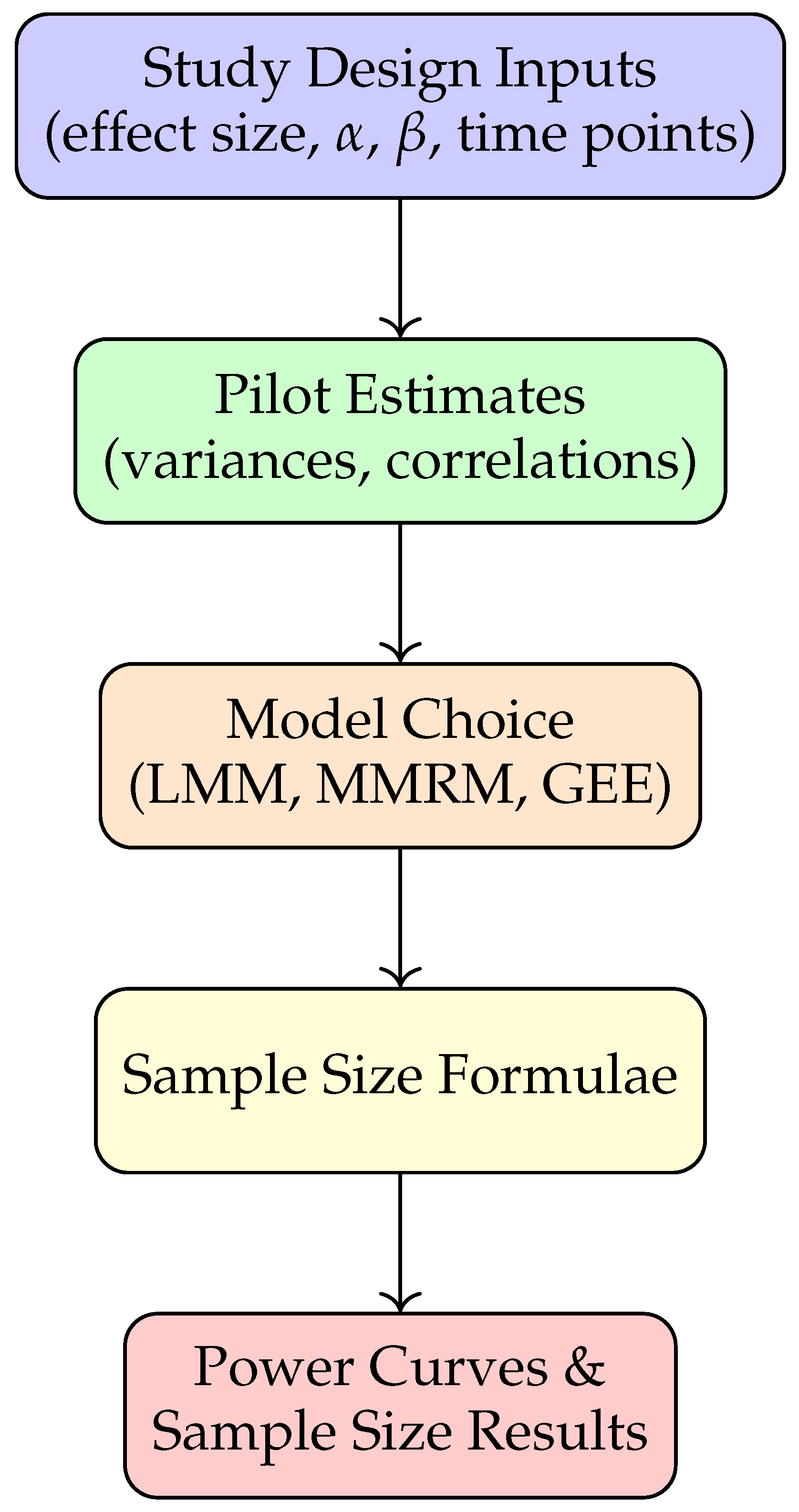
Figure 3.
Sample size vs. correlation under varying variances.
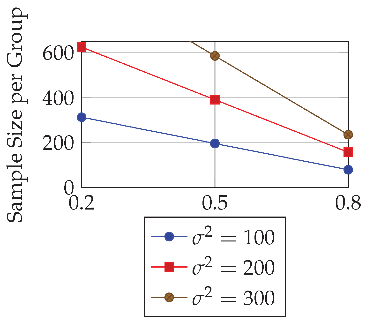
Table 2.
Comparison of LMM, MMRM, and GEE approaches
| Model | Key Assumptions | Applications |
|---|---|---|
| LMM | Linear trajectory; random intercepts/slopes | Continuous outcomes, slope comparisons |
| MMRM | Time categorical; unstructured covariance | Clinical trials with dropout, flexible means |
| GEE | Marginal mean model; working correlation | Binary/ordinal outcomes, population effects |
Table 3.
Required per-group sample sizes under varying assumptions
| Correlation | |||
|---|---|---|---|
| 313 | 625 | 938 | |
| 196 | 391 | 586 | |
| 79 | 157 | 235 |
Disclaimer/Publisher’s Note: The statements, opinions and data contained in all publications are solely those of the individual author(s) and contributor(s) and not of MDPI and/or the editor(s). MDPI and/or the editor(s) disclaim responsibility for any injury to people or property resulting from any ideas, methods, instructions or products referred to in the content. |
© 2025 by the authors. Licensee MDPI, Basel, Switzerland. This article is an open access article distributed under the terms and conditions of the Creative Commons Attribution (CC BY) license (http://creativecommons.org/licenses/by/4.0/).
Copyright: This open access article is published under a Creative Commons CC BY 4.0 license, which permit the free download, distribution, and reuse, provided that the author and preprint are cited in any reuse.


