
Submitted:
23 November 2025
Posted:
24 November 2025
You are already at the latest version
Abstract
The sequence space of all real-valued sequences, denoted Seq(R), is typically investigated through the lens of infinite-dimensional vector spaces, utilizing Banach space norms or Schauder bases. This work proposes a complementary, constructive classification based instead on the asymptotic limit profile encoded by the pair lim infan, lim supan. We demonstrate that this perspective naturally partitions Seq(R) into seven mutually disjoint macroscale blocks, covering behaviors from finite convergence to bounded and unbounded oscillation. For each block, we provide explicit closed-form representative sequences and establish that every constituent class possesses the cardinality of the continuum. Furthermore, we investigate the structural relationships between these blocks at two distinct levels of granularity. At the macroscale, we employ injective mappings to define an idealized connectivity graph, while at the microscale, we introduce a connection relation governed by the Hadamard (pointwise) product. This dual analysis reveals a rich directed graph structure where the block of finite convergent sequences functions as a global attractor with no outgoing connections. Statistical comparisons between the idealized and realized adjacency matrices indicate that the pointwise product structure realizes approximately two-thirds of the theoretically possible macroscale relations. Ultimately, this partition-based framework endows the seemingly chaotic space Seq(R) with a transparent, geometrically interpretable internal structure.
Keywords:
convergent sequences
; divergent sequences
; sequence spaces
; limits
; digraphs
MSC: 40A05; 46A45; 26A03; 05C20
“Mathematics is the science of the infinite, its goal the symbolic comprehension of the infinite with human, that is finite, means.—Hermann K.H. Weyl (1885—1955)
1. Introduction
1.1. Real Valued Sequences
The systematic study of real-valued sequences emerged as a cornerstone of modern real analysis during the nineteenth century. While infinite processes had appeared implicitly in the work of Newton and Leibniz, it was the shift toward rigor, initiated by Cauchy and later clarified by Weierstrass and others, that placed sequences of real numbers at the heart of the theory of limits and convergence (see, e.g., [1,2]). Sequences provided a flexible language to express approximation, to formulate the Cauchy criterion, and to capture completeness properties of the real line. Historical studies of this transition document how the step from intuitive infinitesimals to – arguments was largely mediated by sequences and series [1,2].
In contemporary real analysis, real-valued sequences and their series are treated as one of the primary objects of study, alongside real numbers and real-valued functions. Standard texts typically devote early chapters to basic notions such as boundedness, monotonicity, subsequences, and Cauchy sequences, and then develop fundamental theorems including the Bolzano–Weierstrass theorem and the equivalence between Cauchy and convergent sequences in [3,4,5,6]. These results not only underpin the rigorous development of calculus but also guide later topics such as series, metric spaces, and functional analysis. Introductory treatments by authors such as Tao, Hunter, Deshpande, Loku and Braha, and others all emphasize sequences as the natural setting in which students first encounter the interplay between algebraic structure, order, and completeness [3,4,5,6].
1.2. Motivation
The sequence space of all real-valued sequences on the natural numbers, often denoted or , is an infinite-dimensional vector space with an extremely rich internal structure. As a set of functions , it contains the familiar convergent and Cauchy sequences that encode limits and completeness, but it also hosts a vast collection of divergent, oscillatory, and highly irregular sequences. From the standpoint of cardinality, has the size of the continuum and admits Hamel bases that are necessarily uncountable and nonconstructive; from the analytic standpoint, familiar Banach sequence spaces such as , , and arise as distinguished linear subspaces equipped with norms and (often) countable Schauder bases [3,6].
Because of this breadth, many classical approaches focus on particular “regular” subspaces or impose additional structural conditions: one may restrict attention to bounded or monotone sequences, Cauchy sequences, or sequences belonging to or ; alternatively, one may classify sequences through summability methods (such as Cesàro or Abel summation), through topological properties in metric or product topologies, or through measure-theoretic or probabilistic considerations in the study of random sequences [3,4,5]. These viewpoints have been extremely successful, but they typically either narrow the focus to specific well-behaved classes or rely on infinite expansions with respect to a chosen basis.
The present work proposes a complementary, constructive description of that does not depend on a particular Hamel or Schauder basis. This approach has been previously applied in the case of function space [7]. Instead, we organize sequences according to their asymptotic “limit profile,” encoded by the pair , and show that this perspective leads to a finite partition of into seven macroscale blocks. Within and between these blocks we then investigate finer “connection” relations that reflect how sequences can be transformed into one another while preserving or modifying their limit behaviour. In this way, the enormous and seemingly chaotic space acquires a more transparent, geometrically interpretable structure that complements existing classification schemes based on topology, summability, or basis representations.
1.3. Study Outline
This paper is organized into three main sections. In Section 2 we collect the requisite background from set theory, linear algebra, and the theory of special classes of sequences, providing a common framework for the subsequent analysis. Section 3 develops the central results: we construct a finite partition of the sequence space into seven blocks, supply explicit representatives for each block, and then analyze the relationships between these blocks at both a macroscale and a microscale level using a directed graph viewpoint. Finally, Section 4 offers a discussion of the main findings, highlights the structural insights gained from this partition-based perspective, and outlines several directions for future work.
2. Preliminaries
The reader who has studied linear algebra and real analysis is well equipped with the following set of definition, propositions, theorems and remarks regarding infinite sequences.
2.1. Set-Theoretic Foundations
In this subsection we recall basic set-theoretic notions and standard properties of real-valued sequences that will be used throughout the paper. Our goal is to fix notation and to highlight the central role of the limit inferior and limit superior in describing the long–run behaviour of a sequence.
Definition 2.1
(Sequence space ). We denote by
the set of all real-valued sequences indexed by the natural numbers. When convenient we write as or .
Definition 2.2
(limit profile of the sequence). Let . For each define the tail infimum and tail supremum
The limit inferior and limit superior of a are given by
with values in the extended real line . We will frequently write
Proposition 2.3.
General properties of lim inf and lim sup: Let and define as in Definition 2.2. Then:
- 1.
- The sequence is non-decreasing and is non-increasing.
- 2.
- For every :
- 3.
-
The limitsalways exist in .
- 4.
- We always have the inequality
Theorem 2.4
(Relationship between lim inf, lim sup, and the usual limit). Let and set
Then the following statements hold:
- (i)
- If the (finite) limit exists and is equal to , then
- (ii)
- Conversely, if , then converges to L, that is,
- (iii)
- If , then the sequence does not converge in ; in this case is either divergent to or oscillatory between at least two distinct cluster values.
Remark 2.5.
In the extended real setting, the values and may be equal to . For example, the sequence satisfies while has and These extremal behaviours will play a role in our later classification of into seven macroscale blocks.
2.2. Linear-Algebraic Foundations
We now recall the linear structure of the sequence space and discuss two complementary notions of basis: the algebraic (Hamel) basis and the topological (Schauder) basis. The former captures the purely set-theoretic size of , while the latter reflects more analytic information in classical Banach sequence spaces.
Definition 2.6
(Vector space structure on ). We regard as a real vector space under pointwise operations: for , in and we define
for all . With these operations, is an infinite-dimensional real vector space.
Definition 2.7
(Hamel basis). Let X be a real vector space. A subset is called a Hamel basis (or algebraic basis) of X if:
- (i)
- The elements of B are linearly independent.
- (ii)
- Every element can be written as a finite linear combination of elements of B; that is,for some , scalars , and distinct .
- If such a set B exists, the cardinality is called the (Hamel) dimension of X.
Remark 2.8
(Cardinality of a Hamel basis of ). It is a classical result in set-theoretic linear algebra (assuming the Axiom of Choice) that the Hamel dimension of as a vector space over is equal to the cardinality of the continuum:
In particular, no countable Hamel basis of exists. From the point of view of concrete analysis, any Hamel basis for is therefore necessarily highly non-constructive.
Definition 2.9
(Schauder basis). Let X be a Banach space over . A sequence is called a Schauder basis of X if for every there exists a unique sequence of scalars such that
with convergence taken in the norm of X. The coefficients are called the (Schauder) coordinates of x with respect to the basis .
Remark 2.10
(Schauder bases in classical sequence spaces). In standard Banach sequence spaces such as () and , the canonical unit vectors
for , form a countable Schauder basis. Thus every element of these spaces can be represented as a convergent infinite linear combination of the .
By contrast, the full sequence space equipped with its natural product topology is not a Banach space and does not admit such a simple Schauder basis. For our purposes, the key point is the contrast between:
- the algebraic viewpoint, where has a Hamel basis of cardinality , and
- the analytic viewpoint, where familiar sequence spaces admit countable Schauder bases describing their elements through convergent series.
- Our classification of into seven macroscale blocks will be constructive and finitary in spirit, and will be independent of any particular choice of Hamel or Schauder basis.
2.3. Special Sequences
Lemma 2.11.
Let be a real sequence with infinitely many zeros. Then and can never both be nor both be . In particular, a can never diverge to .
Proof. This is straightforward consequence of the fact that
□
Lemma 2.12.
Let be a non–zero real sequence which is not eventually zero (i.e. for infinitely many indices n). Then we can construct connectors such that, for the Hadamard (pointwise) product [8]:
the following patterns occur:
- (A)
- has and finite;
- (B)
- has finite ;
- (C)
- has finite and ;
- (D)
- has and .
- Here and denote, respectively, the lim inf and lim sup of the corresponding sequence.
Proof. Let be as in the statement and put
By hypothesis S is infinite; fix an enumeration . For any connector we write for the Hadamard product, i.e. .
- (A–pattern). Define c byThen for all k and for . Hence b has a subsequence equal to and infinitely many zeros, so
- (B–pattern). Split S into two infinite subsequences, for instanceDefine b byand then set whenever , and when . By construction b takes the values infinitely often (and 0 possibly as well), henceso and are finite with .
- (C–pattern). Choose any infinite subsequence and defineand again put when , when . Then while for infinitely many n, so
- (D–pattern). Using the same partition as above, defineand set for , when . Then b has subsequences and , hence
In each case we have explicitly constructed a connector c such that the Hadamard product exhibits the desired pair , which completes the proof.
□
3. Main Results
3.1. Partition of with Scenario Classification & Examples
In this section we adopt a constructive viewpoint on the sequence space by organizing it into three successive themes: (i) the existence of certain canonical “blocks,” (ii) the explicit construction of these blocks, and (iii) the assessment of their size. We begin by partitioning into a finite collection of blocks obtained from the interaction of the two classical notions lim inf and lim sup: two real-valued infinite sequences lie in the same block if and only if they share the same pair , as made precise below. We then turn, in Theorem 3.2, to the question of representation, and ask whether each such block admits at least one explicit infinite sequence in closed form that can serve as its representative. Finally, still within the framework of Theorem 1, we address the cardinality of each block and determine the size of these classes inside the ambient space .
Definition 3.1.
Let with associated limits and respectively. Then, a is equivalent to b asymptotically, denoted by , whenever (i) (ii)
As is easily verified, the relation introduced in Definition 3.1 is an equivalence relation on , and therefore it induces a natural partition of the sequence space into its corresponding equivalence classes.
Theorem 3.2.
The sequence space can be partitioned into seven pairwise disjoint blocks, each of cardinality equal to the continuum .
Proof. Let with and . We distinguish three general situations according to the value of . First, if , then may equal , be a finite real number, or equal (3 possibilities). Second, if , then may coincide with , be a finite real strictly smaller than , or equal (again 3 possibilities). Third, if , then necessarily (1 possibility). Altogether this yields possible configurations, and hence 7 corresponding blocks. These blocks, together with one explicit representative sequence for each, are listed in Table 1. Moreover, a straightforward perturbation of each representative sequence (e.g., adding a constant in ) shows that the cardinality of every block is the continuum .
□
Figure 1 presents the seven blocks introduced in the Theorem3.2:
3.2. The Relationship between the Blocks
In this section we examine how the seven blocks of the sequence space are related at two complementary levels. At a macroscale level, we exploit the fact that all blocks have the same cardinality to construct explicit injections between them, mapping elements of one block into another and vice versa. At a microscale level, we introduce the notion of connection, which we use, whenever possible, to represent elements in a given block as pointwise products of elements drawn from other blocks.
3.2.1. Macroscale
Lemma 3.3
(Injectivity of the coding map). Let be the set of all real-valued sequences. Define a bijection by
Let for . These weights satisfy for every n. For set
and denote
Then the map is injective. In particular, the real number is a unique code for the sequence a.
Proof. Suppose , that is,
If for some m we had , choose the least such m. Then the difference of the two series at index m has magnitude at least , while the tail is strictly smaller than ; this is impossible. Hence for all , so for all because is bijective. Thus is injective, and the real number is a unique code for the sequence a.
□
Theorem 3.4
(Macroscale connection between the seven blocks). Let be the set of all real-valued sequences, and for set as defined above with seven blocks as in Table 1. Then for any two distinct blocks there exists an injective map:
Proof. We discuss the existence of injective maps in three steps as follows:
Step 1: Injective maps from the complement to X. For each target region we define a map:
using only the code and the index n. We list the definitions and their liminf/limsup:
- (i)
-
Target G ().Then is constant, hence in G.
- (ii)
-
Target F ().Clearly , so .
- (iii)
- Target E ().so and .
- (iv)
-
Target D ().Along even indices the sequence tends to ; along odd indices it tends to , so .
- (v)
-
Target C ().Then and , so and , hence .
- (vi)
-
Target B ( ). Defineand setThen and with , so .
- (vii)
-
Target A ().Then and , so and ; hence .
Step 2: Each is injective. In each case, the image sequence determines uniquely:
- For , for any n.
- For , .
- For , .
- For , .
- For , .
- For , .
- For , .
- Thus if , then the corresponding codes coincide: . Since is injective, implies . Hence each is a one-to-one map.
Step 3: Injective maps from Y to X. Given arguments in Step 1 and Step 2, it now sufficient to consider:
Finally, summarizing all implications, the adjacency matrix (rows = source X, columns = target Y) for distinctive pairs is
and concretely:
□
Remark 3.5.
Remark 3.6.
Given any two distinct blocks . Then, by two applications of Theorem 3.4 we have: Consequently:
3.2.2. Microscale
Definition 3.7.
Let . We say that a is connected to b, and write , if there exists a sequence such that , where the pointwise (Hadamard) product is defined by:
Remark 3.8.
If in Definition 3.7 we take c to be the constant sequence , then and the relation reduces to the equivalence relation introduced in Definition 3.1. In this sense, extends the asymptotic equivalence relation .
Remark 3.9.
Definition 3.7 naturally induces a notion of connection between the blocks at the microscale. For any , we say that X is connected to Y, and write , if for every sequence there exists a sequence such that the pointwise Hadamard product belongs to Y.
Theorem 3.10
(Microscale connection between the seven blocks). Let be the set of all real-valued sequences with seven blocks as in Table 1. Then any two distinct blocks are connected at microscale level.
Proof. Step 1: Case Discussion Recall that for we write if for every there exists a connector such that the Hadamard product lies in Y. Our goal is to determine, for each ordered pair of distinct blocks , whether holds.
We shall proceed by fixing the target block Y and then examining all six possible sources .
- Case (finite limit). By definitionGiven any , choose the constant connector . Then for all n, so is the constant zero sequence and hencethat is, . Since a was arbitrary, we obtain for every . Restricting to distinct blocks, all six implications with are true.
- Case (). Herewe need the product to diverge to .
- Positive result. If , then , so eventually. With the constant connector we have , and thereforeso for every . Thus .
- Negative results. By Lemma 2.11, if a sequence has infinitely many zeros then no Hadamard product with it can belong to F (its liminf and limsup cannot both be ). Hence, if a block X contains even one sequence with infinitely many zeros, then : taking that particular witnesses the failure of the definition of .
We can choose such a sequence in each of the following blocks:
- in A: for odd n, for even n. Then , , and a has infinitely many zeros;
- in B: for even n, for odd n, so , ;
- in C: for odd n, for even n, so , ;
- in D: for example , , (), so , ;
- in G: the constant zero sequence has .
- In each case a has infinitely many zeros, so by Lemma 2.11 no connector c can produce . Thus
Therefore, with target , the only true implication among the six distinct possibilities is
- Case (). This is completely symmetric to the previous case. We have
- Positive result. If (so ), the connector gives , henceand so for every . Thus .
- Negative results. We reuse exactly the same “infinitely many zeros’’ witnesses in listed above. For each such a no Hadamard product can have , again by Lemma 2.11. Consequently,
Thus, for target , the only true implication among the six distinct cases is
- Case (, ). HereBy the D–pattern in Lemma 2.12, for every with we can construct a connector c such that satisfieshence . Therefore,
For consider the zero sequence . For any connector c the product is again identically zero, with , so it never lands in D. Hence .
Thus, with , five of the six implications (those with ) are true, and only is false.
- Case (). NowUsing the C–pattern in Lemma 2.12, we can, for every with , construct a connector c such thatso that . Hence
For we again take the zero sequence . For any connector c the product is identically zero with finite upper and lower limits, so and thus . Therefore .
So with the only failure among the six implications is .
- Case (finite ). We haveBy the B–pattern of Lemma 2.12, for each with we can construct a connector c so that, for instance,and hence . Thus
For we again choose . For any connector c, has , so and never in B. Therefore .
With target we therefore get five true implications () and one false implication .
- Case (, finite). Finally,Using the A–pattern in Lemma 2.12, we can, for every with , build a connector c such thatso that . ThereforeRestricting to distinct blocks, this yields for all .
For , the zero sequence once more blocks the implication: for any connector c, has , so it never belongs to A. Hence .
Thus, with target , again five of the six implications (with ) are true and is false.
-
Step 2: Summary of Cases Summarizing all implications, the adjacency matrix (rows = source X, columns = target Y) for distinctive pairs isand concretely:□
Figure 3 presents microscale directed connectivity graph between the seven blocks of the sequence space , where a dark-orange node represents a block and a bold arrow indicates that every sequence in X can be mapped into Y by a suitable Hadamard product with some connector sequence. The diagram highlights the rich bidirectional connectivity among blocks A–F, the mutual link between E and F, and the fact that G is a global attractor with no outgoing connections.
Remark 3.11.
For the building blocks of the sequence space there are 42 distinctive pair connections at macro-level and 28 distinctive pair connections at micro-level, respectively.
4. Discussion
4.1. Summary & Contributions
In this work we introduced a finite partition of the sequence space , the set of all real-valued sequences on , indexed by the pair of values , and we supplied constructive closed-form examples representing each of the seven resulting blocks each with the size of continuum. At the macroscale we described an ideal pattern of admissible relations between these blocks, while at the microscale we investigated the connections actually realized via pointwise products of sequences, showing that this finer structure covers about two-thirds of the macroscale possibilities. The central notion of connection between sequences and between blocks led to a distinctive configuration with 28 realized relations among the seven blocks. Overall, the analysis singles out the block G of convergent sequences as a particularly prominent component of the partition, since at the microscale it is directly connected to every other block corresponding to infinite (non-convergent) behavior.
4.2. Comparison of Macroscale Matrix U versus Microscale Matrix V
We compare the macroscale adjacency matrix U (29), which encodes all idealized block–to–block connections, with the microscale matrix V (32), which records the connections actually realized by our construction. By design, U has ones at every off–diagonal position (42 ones and 7 diagonal zeros), while V has 28 ones. Every one in V appears at a position where U also has a one, so in terms of edge sets of directed graphs we have:
and thus V is a subgraph of U; nothing in V contradicts U, it simply omits some edges.
To quantify this compatibility, we use the standard contingency counts
where the last line corresponds to the diagonal zeros.
First, the “coverage of U by V” (recall) is given by:
This is exactly the fraction of potential connections allowed by U that are actually realized in V.
Second, the “consistency of V with U” (precision) is:
Thus every edge that appears in V is permitted by U; there are no forbidden edges.
Third, the Jaccard similarity of the edge sets is [9,10]:
which in this particular setting coincides with the coverage because .
Taken together, these measures show that V provides a dense, though not exhaustive, microscale realization of the macroscale connectivity encoded by U: it respects all global constraints while omitting roughly one third of the possible connections.
4.3. Limitations & Future Work
The limitations of this work are transparent and, at the same time, suggest several directions for further investigation. To begin with, our partition of the sequence space relies solely on the pair , leaving aside other potentially informative features such as rates of convergence or divergence, oscillatory behavior, periodicity, or the Cauchy property. Moreover, the connection relation introduced in Definition 3.7, which underlies the microscale relationships between blocks, is not an equivalence relation and is therefore only a partial tool for organizing these interactions. Finally, it would be natural to study how the asymptotic equivalence relation of Definition 3.1 shapes both the structure and the number of blocks in our partition, and how this picture changes when the defining ingredients in Definition 3.1 are replaced by alternative properties of real-valued sequences. Such modifications are likely to produce new partitions of with different block structures, opening a range of promising avenues for a more refined representation of the sequence space.
4.4. Conclusions
In conclusion, this work provides a constructive, finite, partition-based description of the sequence space , which is more commonly viewed through the lens of its infinite-dimensional linear structure and associated bases. By organizing real-valued sequences into a small number of asymptotic blocks and supplying explicit representatives for each class, we complement the traditional vector-space perspective with a coarse, yet informative, qualitative classification. In addition, the notion of connection between sequences and between blocks enriches this picture by encoding how elements of different classes can interact via pointwise products, thereby endowing with an additional layer of structural insight beyond its standard linear-algebraic description.
Funding
This research received no external funding.
Institutional Review Board Statement
Not Applicable.
Informed Consent Statement
Not Applicable.
Data Availability Statement
Not Applicable.
Acknowledgments
Not Applicable.
Conflicts of Interest
The author declares no conflicts of interest.
Abbreviations
The following abbreviations are used in this manuscript:
- c: cardinality of the continuum; HamSim: Hamming similarity; JacSim: Jaccard similarity; lim inf: limit inferior; lim sup: limit superior; N: set of natural numbers; R: set of real numbers; Seq(R): sequence space.
References
- Grabiner, J. V. (1981). The origins of Cauchy’s rigorous calculus. MIT Press, Cambridge, MA, USA. ISBN 0-486-43815-5.
- Rogers, R. R., & Boman, E. (2014). How we got from there to here: A story of real analysis. Open SUNY Textbooks, Geneseo, NY, USA. ISBN: 978-1-312-34869-1.
- Deshpande, J. V. (2004). Mathematical analysis and applications: An introduction. Alpha Science International. Harrow, UK. ISBN 1-84265-189-7.
- Hunter, J. K. (2014). An introduction to real analysis. University of California, Davis, CA, USA.
- Loku, V., & Braha, N. L. (2024). Basic concepts of mathematical analysis. Cambridge Scholars Publishing. Lady Stephenson Library, UK. ISBN 978-1-0364-1086-5.
- Tao, T. (2016). Analysis I (3rd ed.). Springer. Hindustan Book Agency, New Delhi, India. ISBN 978-981-10-1789-6.
- Soltanifar, M. (2023). A Classification of Elements of Function Space F(R,R). Mathematics, 11(17), 3715. [CrossRef]
- di Dio, P. J., & Langer, L.-L. (2025). The Hadamard product of moment sequences, diagonal positivity preservers, and their generators. Integral Equations and Operator Theory, 97, 32. [CrossRef]
- Levy, A., Shalom, B. R., & Chalamish, M. (2025). A guide to similarity measures and their data science applications. Journal of Big Data, 12, 188. [CrossRef]
- Shibata, N., Kajikawa, Y., & Sakata, I. (2012). Link prediction in citation networks. Journal of the American Society for Information Science and Technology, 63(1), 78–85. [CrossRef]
- Leskovec, J., Rajaraman, A., & Ullman, J. D. (2020). Mining of massive datasets (3rd ed.). Cambridge University Press. [CrossRef]
- Jamil, H., Liu, Y., Caglar, T., Cole, C. M., Blanchard, N., Peterson, C., & Kirby, M. (2023). Hamming similarity and graph Laplacians for class partitioning and adversarial image detection. In Proceedings of the IEEE/CVF Conference on Computer Vision and Pattern Recognition Workshops (CVPRW) (pp. 590–599). IEEE. [CrossRef]
Figure 1.
Partition of by the -plane, where and , into seven admissible regions labelled satisfying . Each region corresponds to a distinct asymptotic behaviour class of real-valued sequences (finite convergent, finite–finite divergent, and the various one-sided or two-sided infinite cases).
Figure 1.
Partition of by the -plane, where and , into seven admissible regions labelled satisfying . Each region corresponds to a distinct asymptotic behaviour class of real-valued sequences (finite convergent, finite–finite divergent, and the various one-sided or two-sided infinite cases).
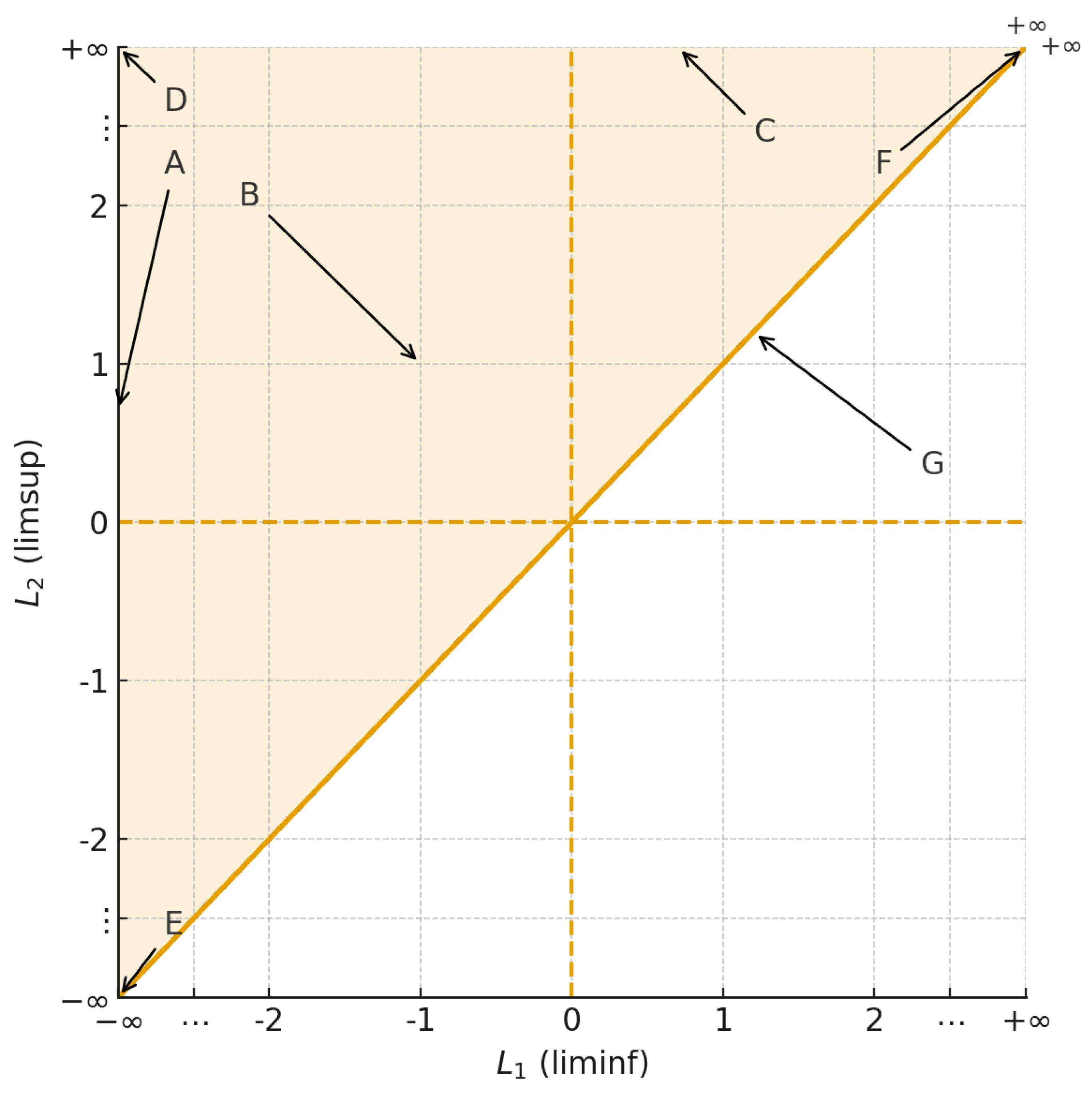
Figure 2.
Heptagon with with macroscale directed connectivity graph between seven blocks (vertices) and directed edges from to G. Each edge is tagged by the global map , while the edge also represents the specific map .
Figure 2.
Heptagon with with macroscale directed connectivity graph between seven blocks (vertices) and directed edges from to G. Each edge is tagged by the global map , while the edge also represents the specific map .
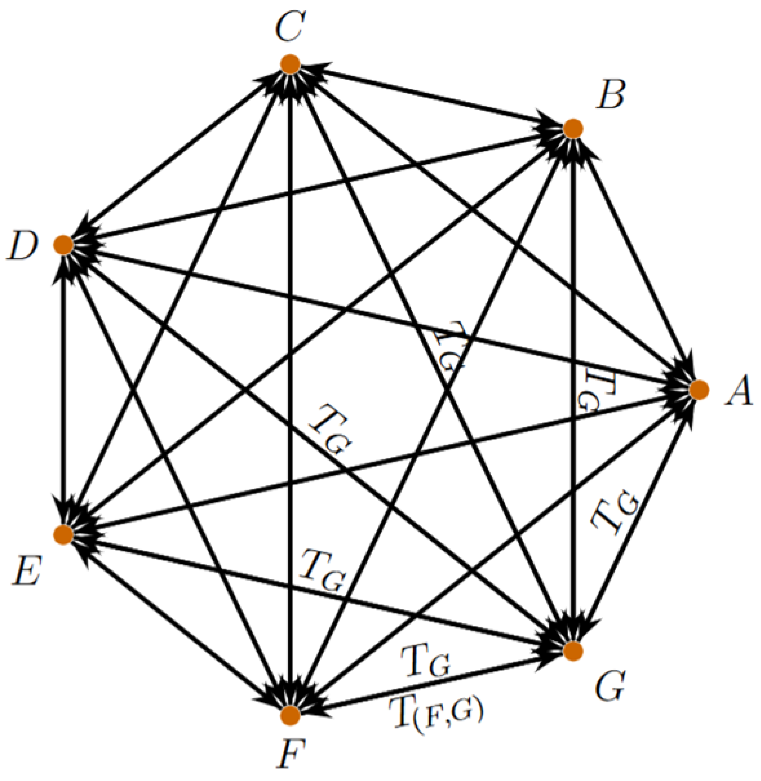
Figure 3.
Heptagon with microscale directed connectivity graph between the seven blocks of the sequence space .
Figure 3.
Heptagon with microscale directed connectivity graph between the seven blocks of the sequence space .
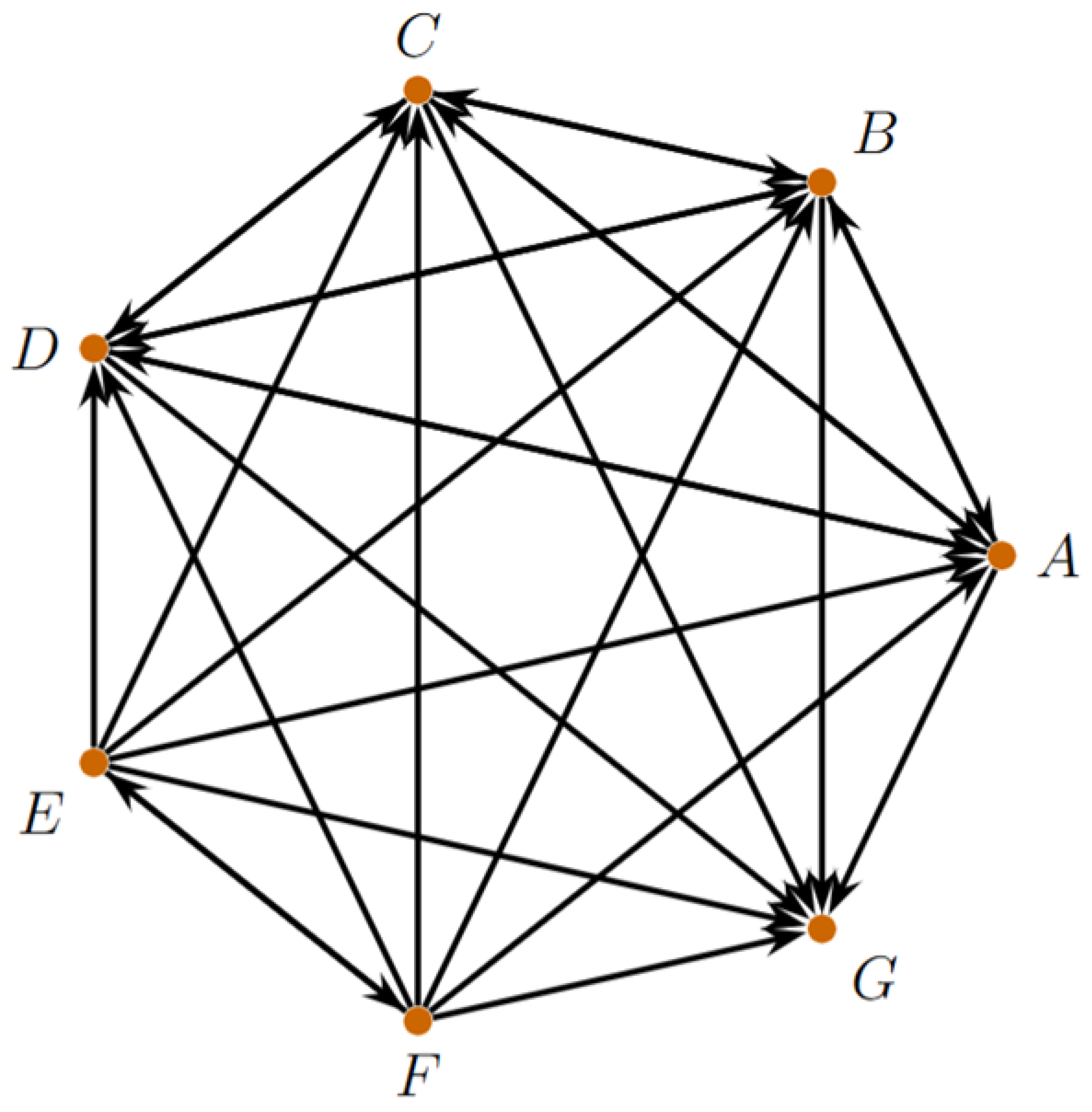

Table 1.
List of seven representatives blocks of partition of with associated representative sequence and size of the block.
Table 1.
List of seven representatives blocks of partition of with associated representative sequence and size of the block.
| # | Block | Definition of | Representative sequence | Size |
| 1 | A | continuum | ||
| 2 | B | continuum | ||
| 3 | C | continuum | ||
| 4 | D | continuum | ||
| 5 | E | continuum | ||
| 6 | F | continuum | ||
| 7 | G | continuum |
Disclaimer/Publisher’s Note: The statements, opinions and data contained in all publications are solely those of the individual author(s) and contributor(s) and not of MDPI and/or the editor(s). MDPI and/or the editor(s) disclaim responsibility for any injury to people or property resulting from any ideas, methods, instructions or products referred to in the content. |
© 2025 by the authors. Licensee MDPI, Basel, Switzerland. This article is an open access article distributed under the terms and conditions of the Creative Commons Attribution (CC BY) license (http://creativecommons.org/licenses/by/4.0/).
Copyright: This open access article is published under a Creative Commons CC BY 4.0 license, which permit the free download, distribution, and reuse, provided that the author and preprint are cited in any reuse.


