
Submitted:
23 November 2025
Posted:
25 November 2025
You are already at the latest version
Abstract
Aiming at improving convergence rate and path feasibility of traditional Rapidly-exploring Random Tree algorithm (RRT), this paper proposed an enhanced RRT with heuristic search (AHRRT). The AHRRT cooperated four strategies: Adaptive step size, Target Bias, Attraction-repulsion strategy and a pruning operation. First, Adaptive step size strategy helps reduce collisions caused by large step sizes and improve the feasibility and safety of the path. Second, Target Bias strategy enhances tree expansion efficiency by directing the search tree toward the target, reducing computational overhead. Third, Attraction-repulsion strategy helps improve obstacle avoidance ability, making the path smoother and avoiding oscillations or invalid sampling caused by large step sizes. Finally, the pruning strategy can further optimize the initial path by removing redundant nodes. Simulation experiments in 2D and 3D validate the effectiveness of AHRRT, demonstrating significant improvements over traditional RRT, RRT variants, A* and ACO algorithm in terms of path quality, convergence speed, and computational efficiency, especially in complex urban environments, enhancing its practical applicability and feasibility in urban UAV path planning.
Keywords:
rapidly-exploring random tree
; UAV
; heuristic search
; path planning
1. Introduction
Path planning is a fundamental technique for enabling agents to find optimal or suboptimal paths in complex environments, with widespread applications in autonomous vehicles, mobile robotics, and unmanned aerial vehicles (UAVs). The core objective of path planning is to navigate an agent from a starting position to a target destination while satisfying various constraints, such as obstacle avoidance, path length minimization, energy efficiency, or flight time optimization. In recent years, advancements in artificial intelligence, computer vision, and control technologies have driven the evolution of path planning methods, spanning traditional mathematical optimization, sampling-based techniques, heuristic search algorithms, and deep reinforcement learning.
In early research on path planning, mathematical optimization methods, such as dynamic programming (DP), and graph search algorithms were widely used to determine optimal paths. Notably, in 1956, Edsger Wybe Dijkstra proposed the Dijkstra algorithm [44], which is based on weighted graphs and employs a breadth-first search (BFS) approach to guarantee the shortest path between a start and a goal node. However, this algorithm exhibits high computational complexity, particularly in high-dimensional continuous spaces, rendering it inefficient in such scenarios. To address this limitation, Peter Hart et al. introduced the A* (A-star) algorithm in 1968 [2,2]. The A* algorithm builds upon Dijkstra’s method by incorporating a heuristic function to guide the search process more effectively. By leveraging heuristic estimations—such as Euclidean distance or Manhattan distance—the algorithm reduces unnecessary expansions, significantly enhancing path planning efficiency. Despite its strong performance across numerous applications, A* remains computationally expensive and struggles to operate in real-time in high-dimensional environments [2]. In the 1990s, M.H. Overmars et al. proposed the probabilistic roadmap (PRM) method [2], a classic path planning approach particularly suited for robotic motion planning. PRM constructs a global roadmap by randomly sampling the workspace and connecting collision-free nodes to generate a feasible path. While effective in static environments, PRM suffers from limited adaptability in dynamic settings. Additionally, grid-based representation methods, such as the artificial potential field (APF) approach, have been widely applied [2]. The APF method models attractive potential fields to guide agents toward the goal while employing repulsive potential fields to avoid obstacles. Despite its conceptual simplicity and effectiveness, APF is prone to significant drawbacks, including local minima traps and target inaccessibility issues. In recent years, with the advancement of computational power and intelligent algorithms, path planning methods have increasingly integrated metaheuristic optimization algorithms and deep learning techniques. Common metaheuristic optimization algorithms include Genetic Algorithm (GA) [2], Particle Swarm Optimization (PSO) [2], Ant Colony Optimization (ACO) [9], and Artificial Bee Colony (ABC) [10]. These algorithms perform global search by simulating biological behaviors and can effectively find near-optimal solutions . However, metaheuristic algorithms often struggle to balance exploration and exploitation, making them prone to local optima [11,12,13,14,15,16,17,18,19]. In 2023, Gang Hu et al. proposed SaCHBA-PDN to enhance the balance between exploration and exploitation in HBA [20]. Experimental results demonstrated that SaCHBA-PDN provided more feasible and efficient paths in various obstacle environments. In 2024, Y. Gu et al. introduced Adaptive Position Updating Particle Swarm Optimization (IPSO), designed to help PSO escape local optima and find higher-quality UAV paths [21]. However, due to its iterative optimization nature, IPSO incurs high computational costs and slow convergence, limiting its applicability in real-time scenarios. Deep reinforcement learning (DRL) has recently emerged as a significant research direction in path planning [22,24]. Reinforcement learning optimizes an agent’s strategy through continuous interaction with the environment during exploration. For instance, path planning methods based on Deep Q-Network (DQN) [23] and Proximal Policy Optimization (PPO) [25] have been applied in autonomous driving and UAV navigation. However, reinforcement learning methods generally require extensive training data, and their generalization ability is constrained by the training environment. Additionally, path planning methods incorporating Simultaneous Localization and Mapping (SLAM) have been widely studied in robotic and UAV navigation [26]. SLAM enables an agent to simultaneously construct a map and plan a path in an unknown environment, making it highly applicable to autonomous driving and robotic navigation. However, SLAM involves high computational complexity, particularly in large-scale three-dimensional environments, where data fusion and real-time processing remain challenging. Among the aforementioned path planning methods, the sampling-based Rapid-exploring Random Tree (RRT) has gained significant attention in recent years due to its efficiency and adaptability [27]. RRT operates by randomly sampling points in the search space and incrementally constructing an expanding tree, enabling rapid coverage of the feasible space. This approach is particularly suitable for path planning in high-dimensional and complex environments. However, traditional RRT algorithms still face several challenges, such as unstable path quality, search efficiency heavily influenced by randomness, and susceptibility to local optima in complex environments. To enhance the performance of RRT in UAV urban path planning, researchers have proposed various improvement strategies. For instance, in 2000, Kuffner J. J. et al. introduced Bidirectional RRT (RRT-Connect), which simultaneously expands tree structures from both the start and goal points, significantly accelerating search convergence [28]. RRT*, an optimized variant of RRT, incorporates a path rewiring mechanism to improve path quality, making it closer to the optimal solution [29]. In 2015, Klemm S. et al. combined the concepts of RRT-Connect and RRT* to propose RRT*-Connect, aiming to provide robust path planning for autonomous robots and self-driving vehicles [30]. In 2022, B. Wang et al. integrated Quick-RRT* with RRT-Connect to develop CAF-RRT*, designed to ensure smoothness and safety in 2D robot path planning [31]. In 2024, Joaquim Ortiz-Haro et al. introduced iDb-RRT to address two-value boundary problems (which are computationally expensive) and to enhance the propagation of random control inputs (which are often uninformative). Experimental results demonstrated that iDb-RRT could find solutions up to ten times faster than other methods [32]. In 2025, Hu W. et al. proposed HA-RRT, incorporating adaptive tuning strategies and a dynamic factor to improve the adaptability and convergence of RRT [33]. However, these methods are often effective in 2D environments, while researchers have largely overlooked the feasibility of applying improved RRT variants to 3D maps. This paper proposed an adaptive RRT algorithm with heuristic search (AHRRT) that integrates heuristic search strategies to enhance the efficiency and robustness of path planning. AHRRT leverages environmental information during the sampling process to adjust the sampling strategy, enabling more efficient path searches in 3D maps. Furthermore, the algorithm incorporates an adaptive adjustment mechanism, allowing the exploration process to dynamically optimize itself based on environmental variations.
2. Structure of the Paper
Section 3 presents the major contributions of this research. Section 4 introduces the traditional RRT algorithm. Section 5 provides a detailed description of the proposed AHRRT algorithm. In Section 6, we compared the proposed AHRRT with RRT variants and other state-of-the-art algorithms in different maps to demonstrate the superiority of AHRRT. Section 7 concludes the research and provides prospects for future research.
3. Major Contribution
To enhance the convergence speed and path feasibility in 3D path planning of the traditional RRT algorithm, this paper proposed an adaptive RRT algorithm with heuristic search (AHRRT). AHRRT integrated four key strategies: an attraction-repulsion strategy, a heuristic target-biasing strategy, a dynamic step-size strategy, and a pruning strategy. First, the attraction-repulsion strategy and the heuristic target-biasing strategy guide the search tree toward the target, improving tree expansion efficiency and thereby reducing computational overhead. Second, the dynamic step-size strategy adaptively adjusts the expansion step size based on repulsion force calculations, enhancing convergence speed. Finally, the pruning strategy optimizes the initially obtained path by removing redundant nodes, ensuring higher path feasibility. The effectiveness and feasibility of AHRRT were validated through simulations on both 2D and 3D maps. The results demonstrate that AHRRT significantly outperforms traditional RRT, RRT variants, A*, and ACO algorithm in terms of path quality, convergence speed, and computational efficiency. Notably, in complex urban environments, AHRRT enhances the practical applicability and feasibility of UAV path planning in urban settings.
4. Rapid-Exploring Random Tree (RRT)
Rapidly-exploring Random Tree (RRT), proposed by LaValle and Kuffner in 1998, is an efficient sampling-based path planning algorithm [27]. Initially developed for high-dimensional path planning, RRT can generate feasible paths from a starting point to a target under complex constraints. The design of RRT addresses the computational complexity faced by traditional methods in high-dimensional and obstacle-rich spaces. Given its efficient exploration capabilities, RRT has been widely applied in robotic motion planning, autonomous driving, UAV navigation, and medical robotic arm navigation. The core concept of RRT is to gradually grow a tree-like structure in the state space through random sampling, dynamically expanding the tree nodes to cover the free space. As shown in Figure 1, the root node of the RRT tree is the starting point. A random sample point is generated with a uniform probability distribution, and the nearest node is identified. Extending towards by one step yields a new node . If is within feasible space, it is added to the tree. When is sufficiently close to the goal or meets a termination criterion, a feasible path from the start to the goal is found, and the algorithm terminates. Figure 2 presents the workflow of RRT and Algorithm 1 is the pseudo-code of RRT.
The sampling strategy of RRT enables rapid, uniform exploration of unknown spaces, making it highly efficient in free space coverage. Figure 3 shows an RRT-planned path on a 2D map. RRT’s performance in high-dimensional and obstacle-dense environments is exceptional, particularly suited for real-time applications. However, RRT has notable limitations:
- Path quality: The generated paths are not optimal and tend to be winding.
- Lack of convergence: RRT does not guarantee an optimal solution and may fail to find the shortest path in complex environments.
- Non-deterministic quality: RRT’s randomness can result in unstable path quality and, with limited samples, may not find a solution.
To address these limitations, this paper introduced an enhanced RRT (AHRRT) to facilitate rapid path planning for the UAV.
| Algorithm 1:RRT |
|
5. AHRRT
5.1. Adaptive Step Size
In the original RRT, the step size is fixed, which may result in missing more optimal paths during the extension process. The step size is fixed, as shown in Figure 4. However, when the tree nodes extend with a fixed step size, if collides with an obstacle, the tree abandons this choice, which is unsuitable for extending the tree in narrow passages. This rigid strategy may lead to the tree missing better paths during the extension process. Therefore, to address the limitation of RRT in passing through narrow passages, this paper proposes an Adaptive Step Size strategy, as shown in Eq. 1. As shown in Figure 5, in the Adaptive step size strategy, the step size automatically decreases when approaching obstacles, reducing collisions caused by an excessively large step size, enabling effective detailed exploration, and improving the feasibility and safety of the path. When moving away from obstacles, the step size remains consistent with the original step size, allowing for efficient exploration.
where is the step size of RRT; is the Euclidean distance of and .
5.2. Target Bias
The standard RRT algorithm generates new nodes through random sampling, expanding the search tree across space. However, this randomness, while fostering exploration diversity, can lead to inefficiencies, particularly in high-dimensional or complex environments where RRT may converge slowly due to local optima. Enhancing RRT’s convergence efficiency and its search capacity toward the goal is a critical area for improvement. The Target Bias strategy addresses these shortcomings by introducing Target Bias strategy, which, with a certain probability, selects the goal point as the sample point, thus increasing the likelihood that the search tree directly extends toward the target [34]. In AHRRT, a probability parameter controls the intensity of the target bias. Specifically, as shown in Equation (4), with a probability of , the target point is directly set as the sample coordinate, thereby guiding the tree to expand toward the goal. If this probability is not met, a random sample is selected to maintain exploration diversity. The introduction of the target bias strategy largely overcomes RRT’s tendency for lengthy paths and slow convergence due to purely random sampling. By creating a guiding effect toward the target, the search tree extends more directly in the goal’s direction, significantly reducing the time needed to find a feasible path. Furthermore, this strategy reduces unnecessary path extensions during the search process, preventing the tree from aimlessly wandering near the target, thus lowering computation costs and improving search efficiency. In practical applications, target bias increases search density near the target, enhancing local search efficiency. This strategy demonstrates significant advantages in convergence and computational efficiency.
Where is the target node coordinate; is the goal bias probability, set to 0.5; is a random number between [0, 1]; represents a randomly generated node.
5.3. Attraction-Repulsion
The Artificial Potential Field (APF) method is a commonly used optimization strategy for robot path planning [2]. The fundamental idea is: (a) The goal point exerts an attractive force on the agent, guiding it towards the target; (b) Obstacles exert a repulsive force on the agent to avoid collisions; (c) The resultant force (attraction + repulsion) determines the direction and step size of the agent’s movement. During the planning process, the agent’s movement direction and step size are adjusted based on the resultant force, thus avoiding obstacles and ultimately reaching the target. We integrate the concept of APF into the Rapidly-exploring Random Tree (RRT) algorithm, proposing the APF-based Attraction-Repulsion strategy to dynamically adjust the step size and sampling direction. Traditional RRT algorithms use a fixed step size, which may lead to the following issues: if the step size is too large, it may lack precision and miss feasible paths; if the step size is too small, the computational cost increases, reducing search efficiency. The Adaptive Step Size Adjustment (APF-based Dynamic Step Size) combines the idea of artificial potential fields, dynamically adjusting the step size based on the distance of the robot to the target and the repulsive force from obstacles, effectively compensating for the shortcomings of a fixed step size.
5.3.1. Attraction Force
Attraction Force from :
Attraction Force from :
where is the attraction force coefficient, set to 1 in this research.
5.3.2. Repulsion Force
where is the repulsive force coefficient, set to 1 in this research.
5.3.3. Total Force
When the node is far from the target, the step size increases, thereby speeding up the search. When the node is close to an obstacle, the step size decreases, improving obstacle avoidance and making the path smoother.
5.4. Pruning Operation
The core idea of the pruning operation is to optimize the path based on collision detection by removing redundant path points, reducing bends, and making the path smoother and more efficient. It optimizes the path by attempting to directly connect non-continuous path points, as shown in Figure 6. If there is no collision during the connection, intermediate points are skipped, thus reducing the number of path points. The pruning operation eliminates unnecessary turning points and skips unnecessary intermediate points, making the optimized path simpler, smoother, and more feasible.
| Algorithm 2:AHRRT |
|
6. Qualitative Experiment
The experimental setup for this study includes a Windows 11 (64-bit) operating system, an Intel(R) Core(TM) i5-8300H CPU @ 2.30GHz processor, and 8GB of RAM. The simulation platform used is MATLAB R2023a.

Table 1.
Details of the experimental setup in this study
| Simulation environment | Setting | |
|---|---|---|
| Hardware | ||
| CPU | i5-8300H CPU @ 2.30GHz | |
| RAM | 8GB | |
| SSD | 1TB | |
| Software | ||
| System | Windows 11 (64-bit) | |
| Platform | Matlab R2023a |
6.1. Parameter Sensitivity Analysis Experiment
In the Target Bias mechanism, the probability p controls the balance between exploration and exploitation in the AHRRT algorithm. When p is set to a low value (e.g., 0.1), the algorithm tends to favor global exploration, exhibiting higher randomness. This may increase the convergence time but helps avoid local optima. Conversely, when p is set to a high value (e.g., 0.9), the algorithm is more inclined to exploit known high-quality solutions, which can accelerate convergence but may lead to premature convergence to a local optimum. Therefore, conducting a parameter sensitivity analysis experiment is crucial. Through this experiment, we determine the optimal value of p that enables AHRRT to achieve optimal performance across different application scenarios. Due to the randomness of the RRT algorithm, we ran it multiple times to minimize the interference of randomness as much as possible. We created six 1000x1000 maps with obstacles of varying densities, as shown in Figure 7, and ran AHRRTs with different p values(0.1, 0.3, 0.5, 0.7, 0.9) 50 times on each map. We recorded the path lengths, running times, waypoints and number of nodes to to comprehensively select the most suitable parameter p for AHRRT, so that AHRRT performs optimally in different scenarios. As shown in Table 2, Table 3, Table 4 and Table 5, as the value of p increases, the path length obtained by AHRRT decreases to a certain extent. Particularly in simpler scenarios, the convergence speed of AHRRT can be effectively accelerated as p increases. However, in more complex scenarios, the computational time increases significantly, which is undesirable. For example, in Map6, compared to AHRRT(p=0.1), AHRRT(p=0.5) reduced the path length by 0.1%, but the computational time increased by 37.30%. Meanwhile, AHRRT(p=0.9) reduced the path length by 0.8%, but the computational time increased by 1008.11%, which is unacceptable. After considering all factors, we chose p=0.5.
6.2. Ablation Study
In this ablation study, we removed the three improvement strategies respectively from AHRRT to evaluate the impact of each improvement strategy on AHRRT. Since the pruning operation is a path optimization strategy, it is not evaluated in the ablation study.
- AHRRT1: We replaced the Adaptive step size strategy in AHRRT with fixed step size, which is referred to as AHRRT1;
- AHRRT2: We replaced the Target bias strategy in AHRRT with the random sampling strategy, referred to as AHRRT2;
- AHRRT3: We removed the Attraction-repulsion strategy in AHRRT, which is referred to as AHRRT3;
As shown in Table 6, Table 7, Table 8 and Table 9, when the obstacle density is low, the effectiveness of the Adaptive Step Size strategy is not significant. However, as the obstacle density increases, the impact of the Adaptive Step Size strategy becomes more pronounced. In high-density obstacle maps, this strategy effectively assists AHRRT in identifying more feasible solutions and exploring higher-quality paths. The Target Bias strategy demonstrates greater effectiveness in low-density environments. Specifically, in Map 1, the introduction of the Target Bias strategy increases the planning speed by 74,175%. In Map 2, it improves planning speed by 17,868%, and in Map 3, the improvement reaches 95,716%. The Target Bias strategy provides heuristic guidance for tree expansion, and its probability-biased mechanism helps AHRRT reduce unnecessary and blind exploration, thereby enhancing computational efficiency and making the planning process more goal-oriented and targeted. The APF-based Attraction-Repulsion strategy aids AHRRT in effectively avoiding obstacles while guiding the tree toward the goal. In maps with low obstacle density, this strategy doubles the convergence speed and significantly improves path quality. In high-density obstacle maps, although the APF-based Attraction-Repulsion strategy continues to enhance path quality, the computation of attractive, repulsive, and resultant forces increases the overall computational load, which in turn leads to a higher planning time consumption.
7. Simulation Experiments
In this section, we selected 2D and 3D maps to verify the superiority and practicality of AHRRT, by comparing it with classical RRT, RRT variants and other SOTA path planning algorithms. The experimental setup for this study includes a Windows 11 (64-bit) operating system, an Intel(R) Core(TM) i5-8300H CPU @ 2.30GHz processor, and 8GB of RAM. The simulation platform used is MATLAB R2023a.
7.1. 2D Maps
We selected traditional RRT, pRRT [35], AVSRRT [36], and AHRRT, and compared them using 2D maps to verify the superiority and practicality of AHRRT. We created six 1000x1000 maps with obstacles of varying densities, and ran RRT, pRRT, AVSRRT, and AHRRT 50 times on each map. We recorded the path lengths and running times to comprehensively analyze the performance of AHRRT. The results indicate that AHRRT achieved better paths across all six maps, demonstrating strong solving capabilities. In terms of planning time, AHRRT was the fastest in solving Map1 to Map5, which suggests that it has a high planning speed. However, when solving Map6, AHRRT performed slower than pRRT. Nonetheless, in terms of path quality, AHRRT significantly outperformed pRRT. This indicates that, although pRRT may have a slightly faster planning speed in more complex environments, its path quality is poor. On the other hand, AHRRT took slightly longer but generated a higher quality path, which is acceptable. In conclusion, AHRRT has a significant advantage in both path quality and planning speed. Figure 14 shows the results of performing the pruning operation on the initial paths. It is worth noting that the path length after pruning is smoother, 17.64% shorter than the initial path. The pruning operation removes redundant nodes, significantly reducing the number of waypoints and turns, making the path more suitable for the actual flight requirements of the drone and effectively reducing its energy consumption.
Figure 8.
Results of the algorithms in Map1.
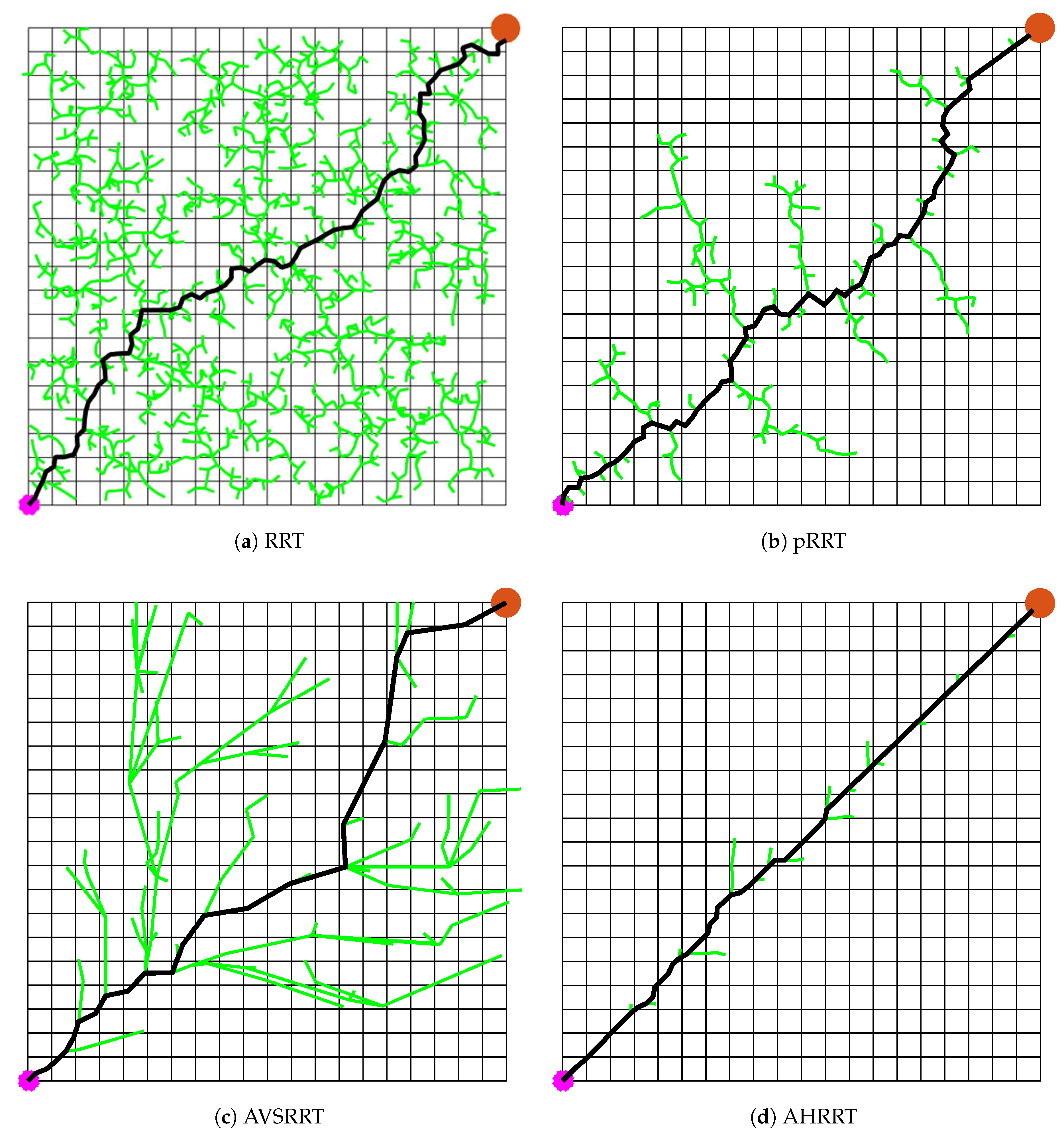
Figure 9.
Results of the algorithms in Map2.
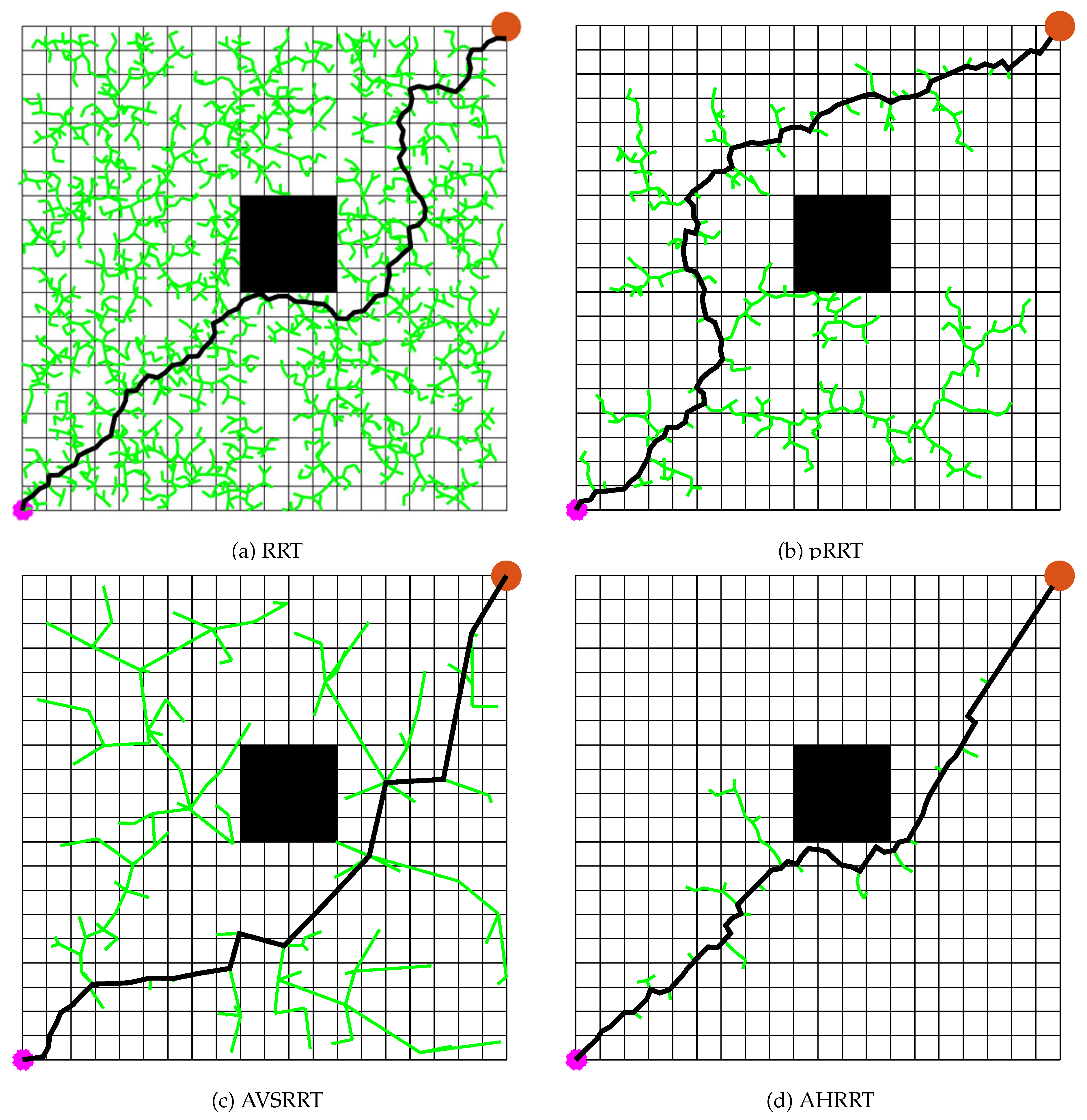
Figure 10.
Results of the algorithms in Map3.
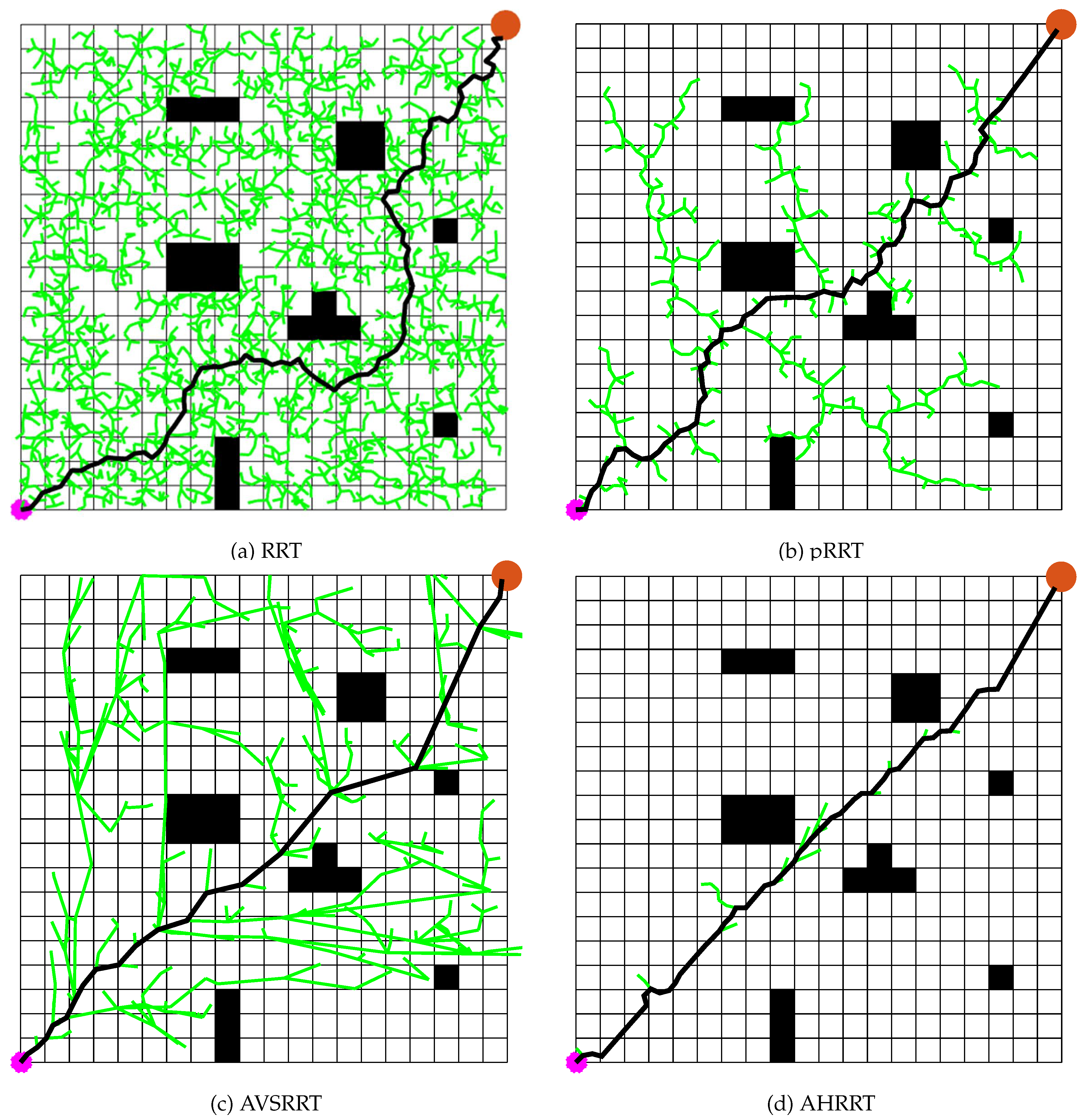
Figure 11.
Results of the algorithms in Map4.
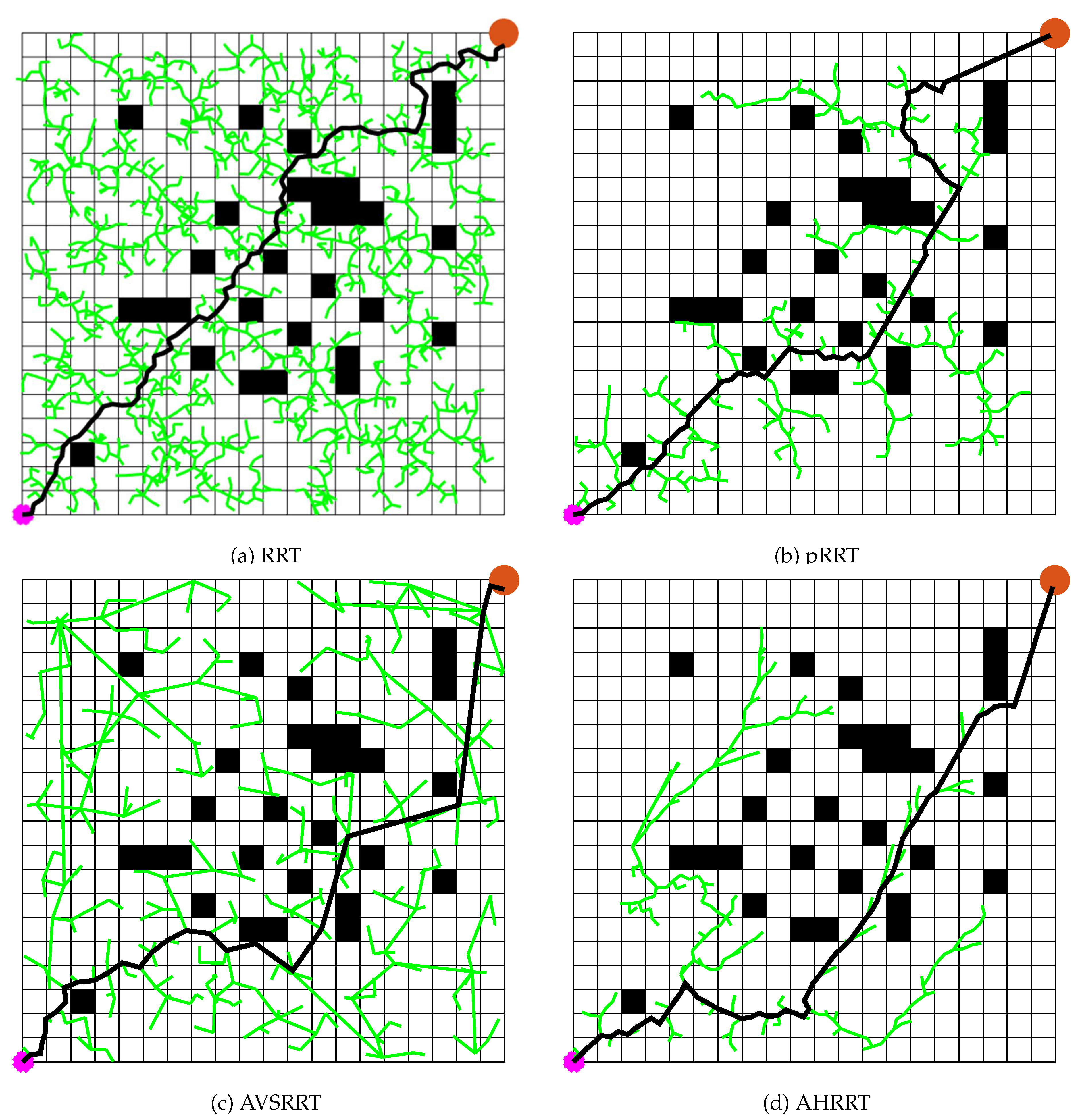
Figure 12.
Results of the algorithms in Map5.
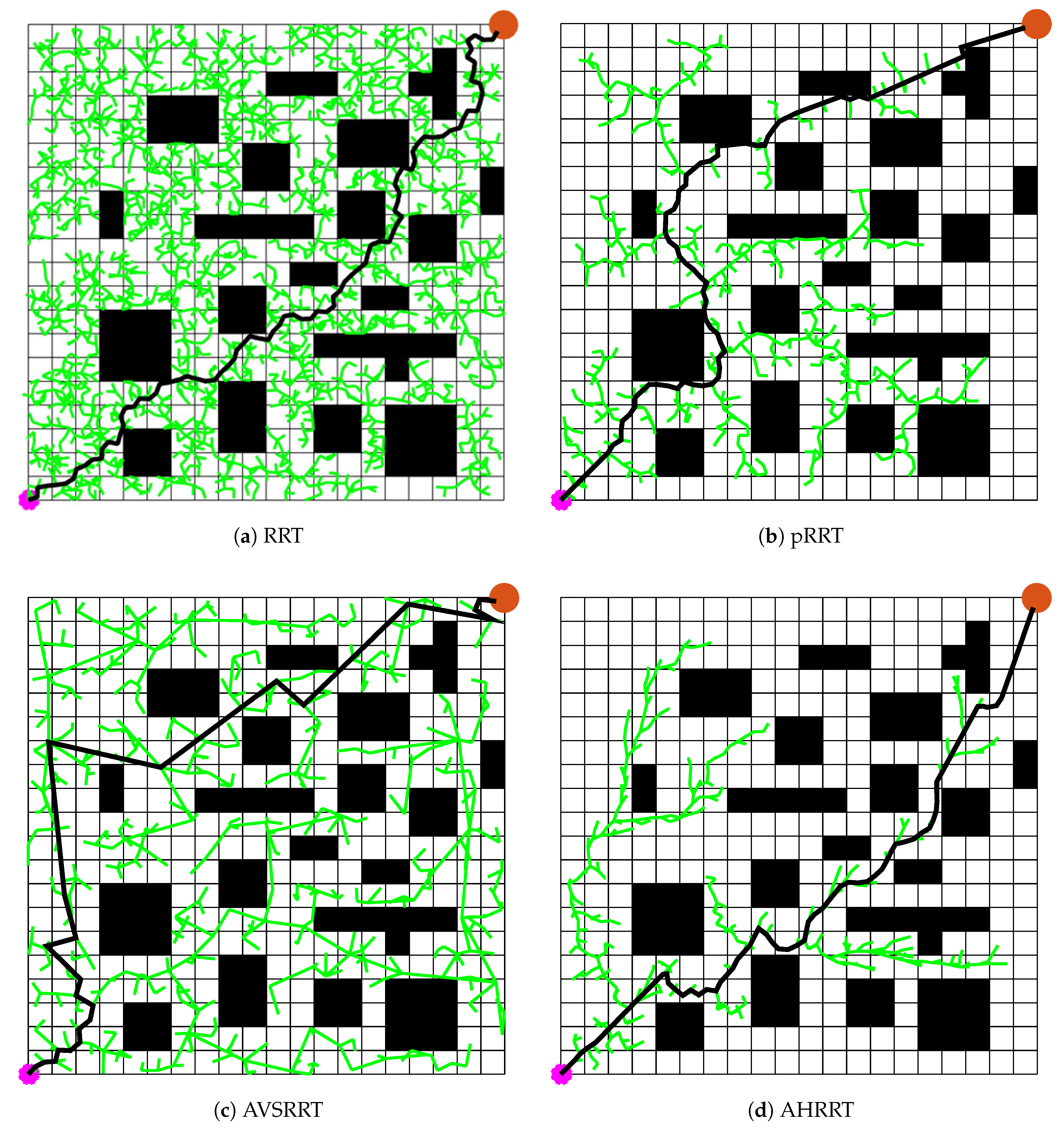
Figure 13.
Results of the algorithms in Map6.
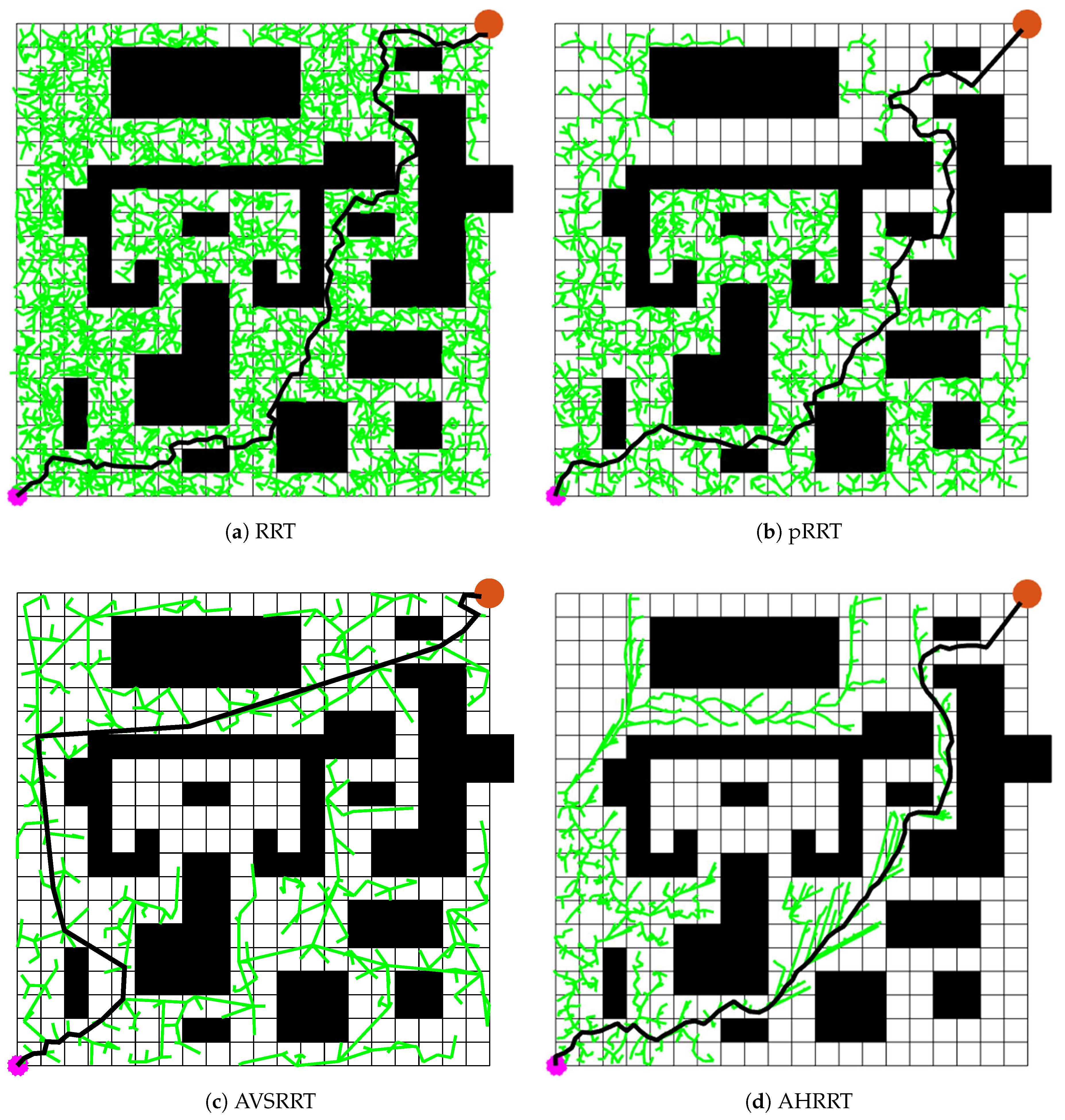
Table 10.
Length of the paths generated by the algorithms in different maps. indicates average length and indicates standard deviation.
Table 10.
Length of the paths generated by the algorithms in different maps. indicates average length and indicates standard deviation.
| Algorithm | Metrics | Map1 | Map2 | Map3 | Map4 | Map5 | Map6 |
|---|---|---|---|---|---|---|---|
| RRT | Ave | 1718.4 | 1815.6 | 1783.2 | 1874 | 1907.6 | 2138.8 |
| Std | 57.26 | 96.91 | 88.0 | 126.44 | 97.11 | 179.18 | |
| pRRT | Ave | 1648.8 | 1721.6 | 1725.2 | 1782.8 | 1750.8 | 2112.4 |
| Std | 48.68 | 71.7 | 93.53 | 81.12 | 104.37 | 166.74 | |
| AVSRRT | Ave | 1633.09 | 2034.68 | 1888.07 | 1873.23 | 1884.73 | 2154.03 |
| Std | 113.13 | 353.76 | 226.34 | 241.04 | 139.64 | 162.4 | |
| AHRRT | Ave | 1423.60 | 1508.81 | 1497.15 | 1626.91 | 1676.09 | 1744.99 |
| Std | 11.91 | 21.66 | 45.48 | 69.25 | 67.01 | 65.55 |
Table 11.
Time consumption of the algorithms in different maps. indicates average time consumption and indicates standard deviation.
Table 11.
Time consumption of the algorithms in different maps. indicates average time consumption and indicates standard deviation.
| Algorithm | Metrics | Map1 | Map2 | Map3 | Map4 | Map5 | Map6 |
|---|---|---|---|---|---|---|---|
| RRT | Ave | 4.7736 | 4.8144 | 4.9075 | 4.2922 | 4.4904 | 6.3393 |
| Std | 4.7988 | 3.2488 | 4.6017 | 2.8774 | 3.0504 | 2.9671 | |
| pRRT | Ave | 0.0822 | 0.1051 | 0.1274 | 0.2593 | 0.4975 | 2.0403 |
| Std | 0.0195 | 0.0246 | 0.0465 | 0.1868 | 0.4732 | 1.3616 | |
| AVSRRT | Ave | 0.888 | 1.2099 | 1.7727 | 2.2485 | 5.7595 | 19.1874 |
| Std | 1.7506 | 1.9252 | 2.9827 | 2.3856 | 3.663 | 11.0457 | |
| AHRRT | Ave | 0.0100 | 0.0366 | 0.0665 | 0.1863 | 0.4011 | 3.0896 |
| Std | 0.0014 | 0.0117 | 0.0433 | 0.1872 | 0.4686 | 2.2848 |
7.2. 3D Urban Maps
In urban path planning, the traditional RRT algorithm can generate a feasible path relatively quickly. However, the generated path often includes significant turns, is overly long, and requires a longer planning time, impacting the practical feasibility and efficiency of UAV flight paths. The proposed AHRRT algorithm aims to improve path quality, speed up planning, reduce large turns along the path, and optimize computational efficiency. This experiment aims to demonstrate AHRRT’s advantages in the following aspects: (a) Improved Path Quality; (b) Optimized Computational Efficiency; (c) Enhanced Operability. Figure 16 illustrates the yaw angle; if the yaw angle is less than 45 degrees, the path turn is smoother, making the generated path easier to execute. This section evaluates the performance of the AHRRT through simulation experiments. To comprehensively validate AHRRT’s effectiveness and advantages in urban path planning, we compare it with classical path planning algorithms. We compare it with the traditional RRT algorithm, A* algorithm [2] and Ant Colony Optimization (ACO) algorithm [9] to verify AHRRT’s superior performance.
7.2.1. Mathematical Model for ACO
Metaheuristic algorithm, such as ACO, is widely applied in UAV path planning due to its strong global search ability and robustness in solving complex optimization problems. The basic principle is to model the path planning task as an optimization problem, where the goal is to search for an optimal or near-optimal flight path under multiple constraints (e.g., safety, energy efficiency, smooth maneuvering). By iteratively updating candidate solutions and balancing exploration and exploitation, metaheuristic algorithms can efficiently handle the high-dimensional and nonlinear nature of UAV path planning problems. To evaluate the quality of a candidate path, a comprehensive cost function is constructed as:
where is the cost function of the UAV path planning for ACO; , and are weighting coefficients that balance different objectives, and they comply with the constraints of the folling Eq 11.
In this study, , , and are set to 0.4, 0.3, and 0.3, respectively [21].
- Length Cost (): Since UAVs are required to minimize flight time and reduce energy consumption while ensuring safety, the total path length is a fundamental criterion. A shorter path generally implies lower energy usage and faster arrival.
- Altitude Cost (): UAV flight altitude directly influences both the control stability and operational safety. Excessive altitude changes may increase energy consumption and risk, thus an altitude-related term is incorporated to penalize unnecessary altitude fluctuations.
- Smoothness Cost (): UAV maneuverability is strongly affected by sharp turns and steep climbs/descents. Therefore, the smoothness cost considers both the heading angle change (turning angle) and pitch angle change (climbing angle). This term ensures the generated path is dynamically feasible and reduces the burden on the UAV’s control system.
7.2.2. Parameter Settings
The parameter settings for each algorithm are shown in Table 12.
7.2.3. Simulation Experiment
In this paper, as illustrated in Figure 15, we set the map range to (500m*500m*500m) and simulate the distribution of urban buildings within this area. Rectangular prisms represent buildings of various heights, ranging from 18m to 270m. The start coordinates are set to (10, 10, 1), and the target coordinates are set to (470, 420, 50). Each algorithm was run 50 times in an urban map to eliminate randomness and verify robustness. For each run, we recorded: time t, length l, number of waypoints w, total number of search grids m, search reward rate , maximum yaw angle and frequency n of turning angles exceeding 45°. The results are presented in Figure 17 and Table 13. The results indicate that AHRRT demonstrates outstanding computational efficiency, with an average runtime of 0.01468 seconds, significantly outperforming RRT, A*, and ACO. This highlights the remarkable real-time capability of AHRRT in three-dimensional path planning problems, enabling it to complete path searches within an extremely short time frame. Such efficiency makes AHRRT particularly suitable for time-sensitive applications, such as urban UAV path planning. Among the four algorithms, AHRRT generates the shortest path, indicating that its search strategy is more intelligent and optimized, effectively avoiding redundant search paths and enhancing the efficiency and quality of path planning. Compared to RRT, A*, and ACO, the path length of AHRRT is shorter by 33.86%, 10.66%, and 1.22%, respectively. This demonstrates that AHRRT effectively addresses the deficiency of poor path quality in RRT while maintaining strong competitiveness among advanced path planning algorithms. A reduced number of waypoints implies a smoother path with fewer turning points, thereby decreasing path complexity and facilitating more seamless trajectory tracking for robots or UAVs. Compared to A* and ACO, AHRRT significantly reduces the number of waypoints, suggesting a more optimized path with fewer unnecessary detail points, thereby improving execution feasibility and navigation efficiency. The substantial reduction in the number of search grids in AHRRT indicates its ability to efficiently locate the optimal path without conducting extensive searches like A*. This efficient search strategy allows AHRRT to rapidly identify feasible paths in complex environments while minimizing unnecessary computational overhead, making it highly suitable for resource-constrained environments. A smaller maximum yaw angle signifies a smoother path, avoiding abrupt directional changes and thereby enhancing path feasibility. AHRRT outperforms A* and ACO in terms of maximum yaw angle, indicating that its path planning is more refined, reducing sudden turns and improving feasibility. The lower frequency of excessive turning angles further implies a smoother path with more stable directional changes during navigation. AHRRT exhibits significantly fewer instances of excessive turning angles compared to other algorithms, demonstrating a more natural and fluid path, which is crucial for applications such as UAV navigation and autonomous driving. This contributes to reducing heading adjustments and improving motion stability. Overall, AHRRT exhibits superior computational efficiency, optimal path length, the fewest waypoints, minimal search space consumption, the highest search success rate, and the smoothest path among the evaluated algorithms. Its comprehensive performance surpasses that of RRT, A*, and ACO. In urban environments, AHRRT excels in both computational speed and path quality, particularly standing out in terms of efficiency and path smoothness. AHRRT demonstrates strong competitiveness in path planning applications, particularly in scenarios with high obstacle density and stringent real-time requirements, where it exhibits exceptional adaptability and robustness.
8. Conclusions
This paper proposed an enhanced Rapidly-Exploring Random Tree (AHRRT) for UAV path planning. AHRRT integrates the Adaptive Step Size strategy, Target Bias strategy, APF-based Attraction-Repulsion strategy, and pruning operations to overcome the limitations of traditional RRT algorithms, such as slow convergence, limited solution accuracy, and poor adaptability in complex environments. Two qualitative experiments were conducted: Parameter Sensitivity Analysis helps determine the optimal parameter p to maximize AHRRT’s performance across different scenarios, while the Ablation Study provides a clearer analysis of the impact of each improvement strategy. In simulation experiments, AHRRT was compared against other RRT variants in 2D maps with varying obstacle densities to demonstrate its superiority. Furthermore, AHRRT was evaluated against other state-of-the-art path planning algorithms in 3D urban environments to further validate its effectiveness and efficiency. Experimental results show that AHRRT exhibits excellent planning capability and speed in both 2D and 3D environments, with significant advantages in solution quality and computational efficiency. However, AHRRT also has certain limitations. As a global planner, AHRRT primarily aims to generate an initial feasible path for UAVs and does not address dynamic obstacle avoidance. The integration of the Target Bias strategy significantly enhances convergence speed, but its strong goal-directed nature limits AHRRT’s exploration capability, making it less effective in escaping extreme local optima and navigating complex mazes. Additionally, in high-density obstacle environments, the APF-based Attraction-Repulsion strategy requires traversing all obstacles, leading to a substantial increase in computational cost. Moreover, applying the proposed algorithm from simulation to real-world deployment requires overcoming the sim-to-real gap. Future work will focus on real-world deployment by integrating local path planners (e.g., Dynamic Window Approach) to enable real-time UAV navigation. Additionally, we aim to incorporate more strategies to escape local optima, further enhancing AHRRT’s robustness in challenging environments. By integrating multiple strategies, the proposed AHRRT significantly enhances path planning performance, providing new insights and technological support for efficient autonomous UAV navigation in complex environments.
Author Contributions
Conceptualization, Junhao Wei; methodology, Junhao Wei; software, Junhao Wei; validation, Junhao Wei; formal analysis, Shuai Wu and Junhao Wei; investigation, Ran Zhang; resources, Yapeng Wang and Ngai Cheong; data curation, Junhao Wei; writing—original draft preparation, Junhao Wei; writing—review and editing, Junhao Wei, Xu Yang and Yapeng Wang; visualization, Junhao Wei, Ran Zhang, Shuai Wu, Wenxuan Zhu and Yanzhao Gu; supervision, Zhiwen Wang, Yapeng Wang, Xu Yang and SIO KEI IM; project administration, Yapeng Wang and Xu Yang; funding acquisition, Yapeng Wang and Ngai Cheong.
Funding
This research and the APC was funded by Macao Polytechnic University (MPU Grant no: RP/FCA-03/2022; RP/FCA-06/2022) and Macao Science and Technology Development Fund (FDCT Grant no: 0044/2023/ITP2).
Institutional Review Board Statement
Not applicable.
Informed Consent Statement
Not applicable.
Data Availability Statement
No dataset is used in this reasearch.
Acknowledgments
The supports provided by Macao Polytechnic University (MPU Grant no: RP/FCA-03/2022; RP/FCA-06/2022) and Macao Science and Technology Development Fund (FDCT Grant no: 0044/2023/ITP2) enabled us to conduct data collection, analysis, and interpretation, as well as cover expenses related to research materials and participant recruitment. MPU and FDCT investment in our work (MPU Submission Code: fca.4dda.c349.4) have significantly contributed to the quality and impact of our research findings.
Conflicts of Interest
The authors declare no conflicts of interest.
Abbreviations
The following abbreviations are used in this manuscript:
| Ave | Average fitness |
| Std | Standard deviation |
References
- Wang H, Yu Y, Yuan Q. Application of Dijkstra algorithm in robot path-planning[C]//2011 second international conference on mechanic automation and control engineering. IEEE, 2011: 1067-1069.
- Hart P E, Nilsson N J, Raphael B. A formal basis for the heuristic determination of minimum cost paths[J]. IEEE transactions on Systems Science and Cybernetics, 1968, 4(2): 100-107.
- Chai Y, Wang Y, Yang X, et al. UAVRM-A*: A Complex Network and 3D Radio Map-Based Algorithm for Optimizing Cellular-Connected UAV Path Planning[J]. Sensors, 2025, 25(13): 4052.
- Zhou X, Wang Z, Ye H, et al. Ego-planner: An esdf-free gradient-based local planner for quadrotors[J]. IEEE Robotics and Automation Letters, 2020, 6(2): 478-485.
- Duchoň F, Babinec A, Kajan M, et al. Path planning with modified a star algorithm for a mobile robot[J]. Procedia engineering, 2014, 96: 59-69.
- Kavraki L E, Svestka P, Latombe J C, et al. Probabilistic roadmaps for path planning in high-dimensional configuration spaces[J]. IEEE transactions on Robotics and Automation, 2002, 12(4): 566-580.
- John, H. Holland. Genetic algorithms. Scientific American, 1992; 73. [Google Scholar]
- James Kennedy and Russell Eberhart. Particle swarm optimization. In Proceedings of ICNN’95-International Conference on Neural Networks, 1942; 4.
- Marco Dorigo, Mauro Birattari, and Thomas Stutzle. Ant colony optimization. IEEE Computational Intelligence Magazine, 2006; 39.
- Karaboga D, Akay B. A comparative study of artificial bee colony algorithm[J]. Applied mathematics and computation, 2009, 214(1): 108-132.
- Wei J, Gu Y, Lu B, et al. RWOA: A novel enhanced whale optimization algorithm with multi-strategy for numerical optimization and engineering design problems[J]. PloS one, 2025, 20(4): e0320913.
- Wei J, Gu Y, Yan Y, et al. LSEWOA: An Enhanced Whale Optimization Algorithm with Multi-Strategy for Numerical and Engineering Design Optimization Problems[J]. Sensors, 2025, 25(7): 2054.
- Wei J, Gu Y, Xie Z, Yan Y, Lu B, Li Z, Cheong N, et al. (2025) LSWOA: An enhanced whale optimization algorithm with Levy flight and Spiral flight for numerical and engineering design optimization problems. PLoS One 20(9): e0322058.
- Lu B, Xie Z, Wei J, et al. MRBMO: An Enhanced Red-Billed Blue Magpie Optimization Algorithm for Solving Numerical Optimization Challenges[J]. Symmetry, 2025, 17(8): 1295.
- Wei J, Gu Y, Yan Y, et al. TSWOA: An Enhanced WOA with Triangular Walk and Spiral Flight for Engineering Design Optimization[C]//2025 8th International Conference on Advanced Algorithms and Control Engineering (ICAACE). IEEE, 2025: 186-194.
- Gu Y, Wei J, Li Z, Lu B, Pan S, Cheong N (2025) GWOA: A multi-strategy enhanced whale optimization algorithm for engineering design optimization. PLoS One 20(9): e0322494.
- Wei J, Gu Y, Zhang R, et al. An Enhanced Whale Optimization Algorithm with Log-Normal Distribution for Optimizing Coverage of Wireless Sensor Networks[J]. arXiv:2511.15970, 2025.
- Wu S, Dong A, Li Q, et al. Application of ant colony optimization algorithm based on farthest point optimization and multi-objective strategy in robot path planning[J]. Applied Soft Computing, 2024, 167: 112433.
- Wu S, Li Q, Wei W. Application of ant colony optimization algorithm based on triangle inequality principle and partition method strategy in robot path planning[J]. Axioms, 2023, 12(6): 525.
- Hu G, Zhong J, Wei G. SaCHBA_PDN: Modified honey badger algorithm with multi-strategy for UAV path planning[J]. Expert Systems with Applications, 2023, 223: 119941.
- Wei J, Gu Y, Law K L E, et al. Adaptive Position Updating Particle Swarm Optimization for UAV Path Planning[C]//2024 22nd International Symposium on Modeling and Optimization in Mobile, Ad Hoc, and Wireless Networks (WiOpt). IEEE, 2024: 124-131.
- Liu C H, Chen Z, Tang J, et al. Energy-efficient UAV control for effective and fair communication coverage: A deep reinforcement learning approach[J]. IEEE Journal on Selected Areas in Communications, 2018, 36(9): 2059-2070.
- Koushik A M, Hu F, Kumar S. Deep Q-learning-based node positioning for throughput-optimal communications in dynamic UAV swarm network[J]. IEEE Transactions on Cognitive Communications and Networking, 2019, 5(3): 554-566.
- Gu Y, Wei J, Cheong N. Credit Card Fraud Detection Based on MiniKM-SVMSMOTE-XGBoost Model[C]//Proceedings of the 2024 8th International Conference on Big Data and Internet of Things. 2024: 252-258.
- Zhan G, Zhang X, Li Z, et al. Multiple-uav reinforcement learning algorithm based on improved ppo in ray framework[J]. Drones, 2022, 6(7): 166.
- Schmuck P, Chli M. Multi-uav collaborative monocular slam[C]//2017 IEEE International Conference on Robotics and Automation (ICRA). IEEE, 2017: 3863-3870.
- LaValle, S. Rapidly-exploring random trees: A new tool for path planning[J]. Research Report 9811, 1998. [Google Scholar]
- Kuffner J J, LaValle S M. RRT-connect: An efficient approach to single-query path planning[C]//Proceedings 2000 ICRA. Millennium conference. IEEE international conference on robotics and automation. Symposia proceedings (Cat. No. 00CH37065). IEEE, 2000, 2: 995-1001.
- Karaman S, Walter M R, Perez A, et al. Anytime motion planning using the RRT[C]//2011 IEEE international conference on robotics and automation. ieee, 2011: 1478-1483.
- Klemm S, Oberländer J, Hermann A, et al. RRT*-Connect: Faster, asymptotically optimal motion planning[C]//2015 IEEE international conference on robotics and biomimetics (ROBIO). IEEE, 2015: 1670-1677.
- Wang B, Ju D, Xu F, et al. CAF-RRT*: A 2D path planning algorithm based on circular arc fillet method[J]. IEEE Access, 2022, 10: 127168-127181.
- Ortiz-Haro J, Hönig W, Hartmann V N, et al. idb-rrt: Sampling-based kinodynamic motion planning with motion primitives and trajectory optimization[C]//2024 IEEE/RSJ International Conference on Intelligent Robots and Systems (IROS). IEEE, 2024: 10702-10709.
- Hu W, Chen S, Liu Z, et al. HA-RRT: A heuristic and adaptive RRT algorithm for ship path planning[J]. Ocean Engineering, 2025, 316: 119906.
- Xie Z, Lu B, Gu Y, et al. Research on UAV Applications in Public Administration: Based on an Improved RRT Algorithm[J]. arXiv:2508.14096, 2025.
- Zhang H, Xie X, Wei M, et al. An improved goal-bias RRT algorithm for unmanned aerial vehicle path planning[C]//2024 IEEE International Conference on Mechatronics and Automation (ICMA). IEEE, 2024: 1360-1365.
- An B, Kim J, Park F C. An adaptive stepsize RRT planning algorithm for open-chain robots[J]. IEEE Robotics and Automation Letters, 2017, 3(1): 312-319.
- Xu, G. A comparative study of drones path planning and bezier curve optimization based on multi-strategy search algorithm[J]. PLoS One, 2025, 20(7): e0326633.
Figure 1.
Extension process of RRT.
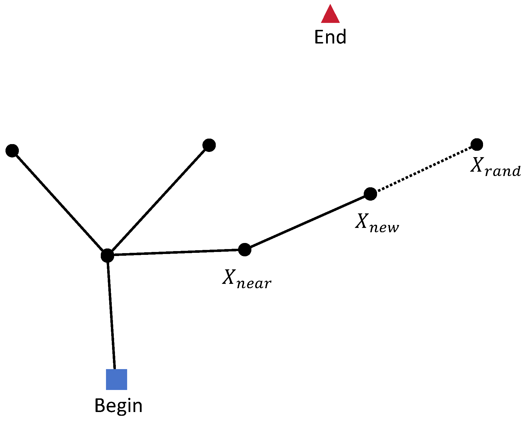
Figure 2.
Workflow of RRT.
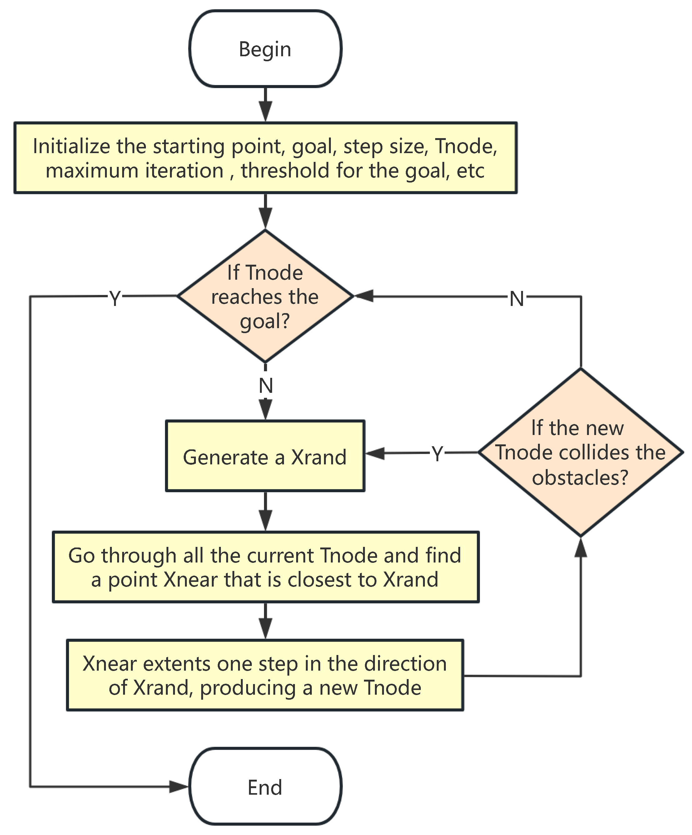
Figure 3.
A path generated by the classic RRT in a 2D map.
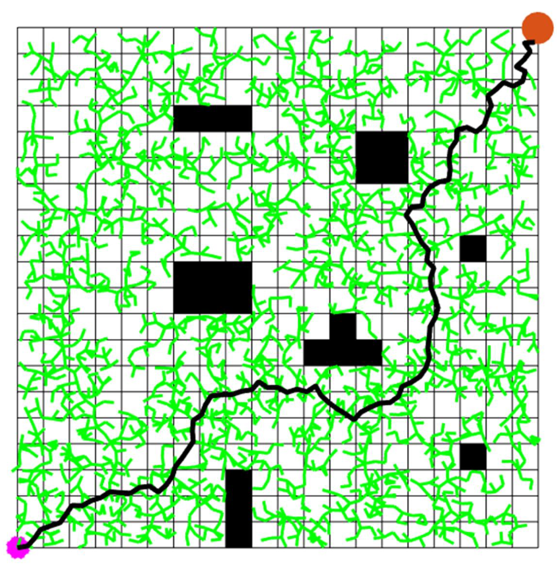
Figure 4.
The fixed step size in RRT.
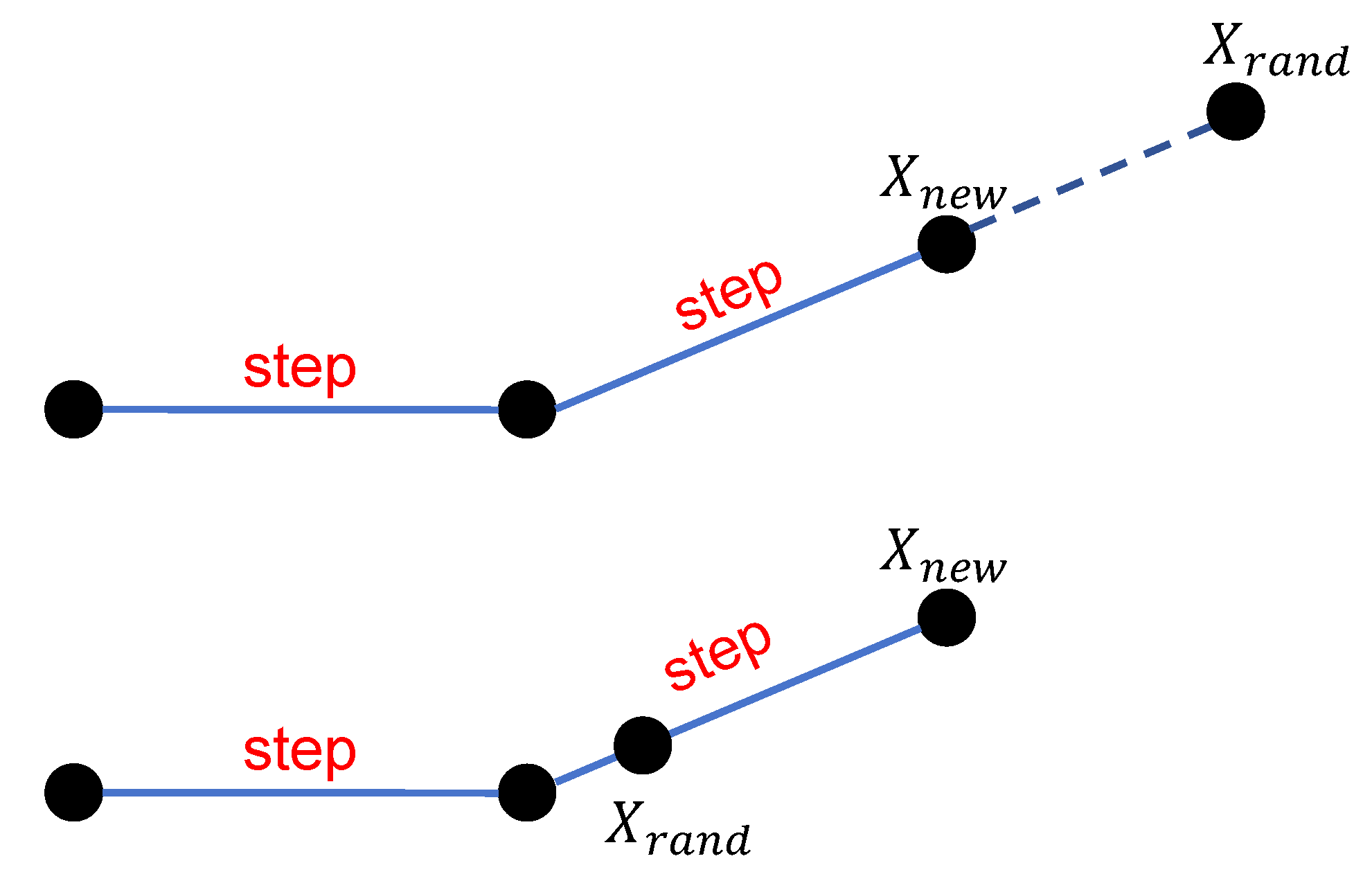
Figure 5.
The adaptive step size in AHRRT.
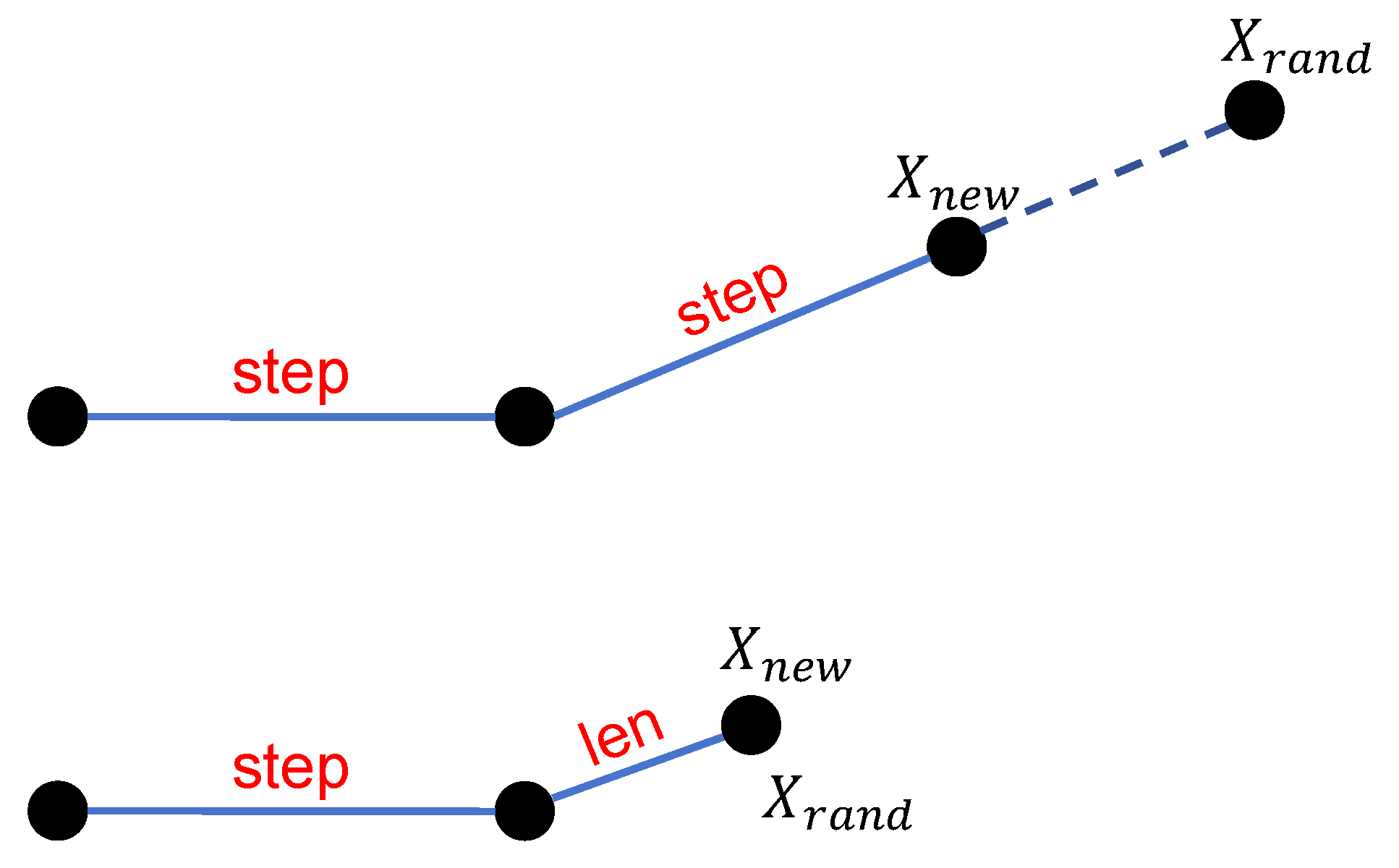
Figure 6.
Pruning operation. The red line is the acceptable shorter path. The yellow line is the unacceptable shorter path because it intersects with an obstacle.
Figure 6.
Pruning operation. The red line is the acceptable shorter path. The yellow line is the unacceptable shorter path because it intersects with an obstacle.
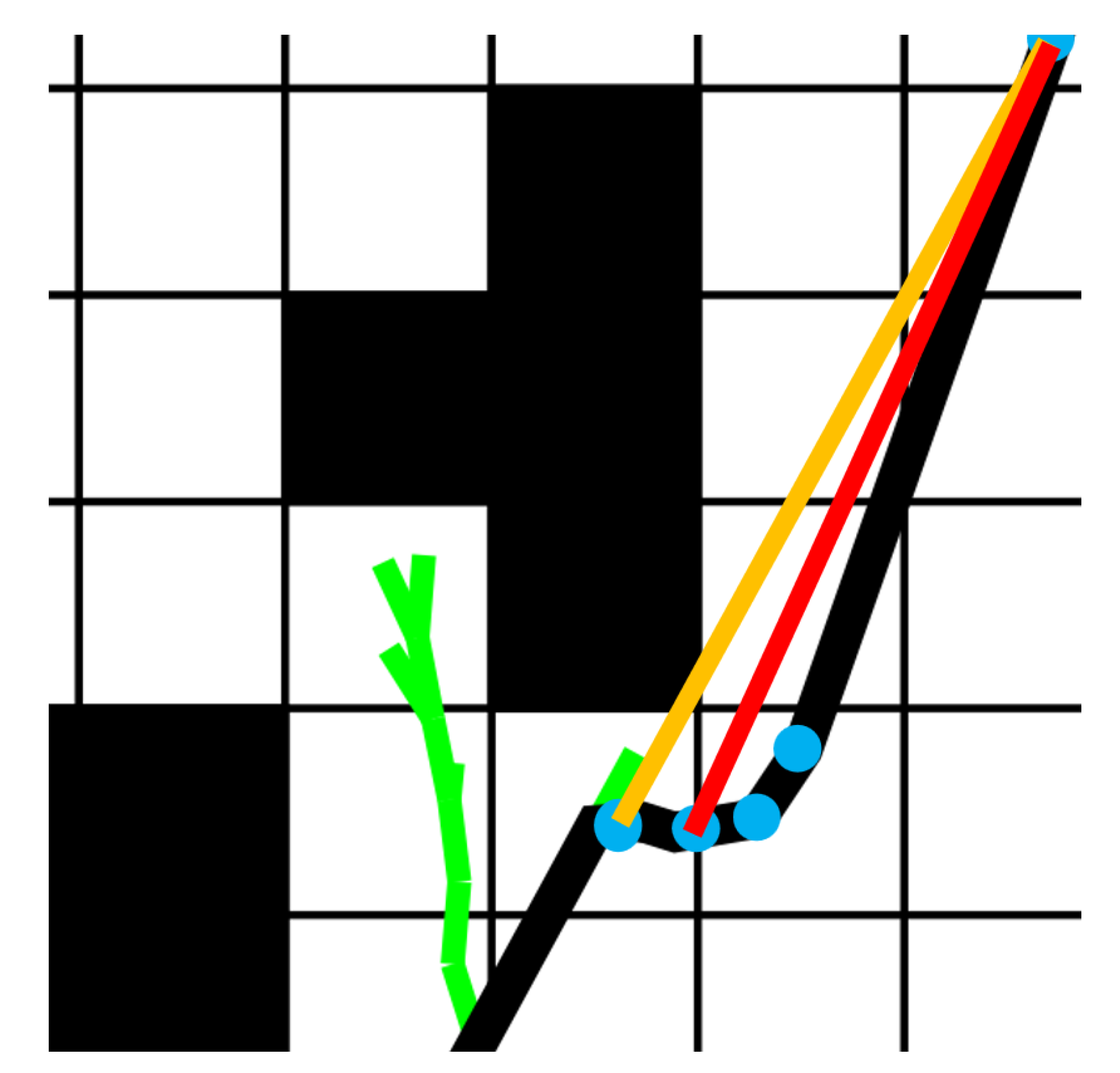
Figure 7.
2D maps with different densities of obstacles. The magenta marker is the starting point, and the orange marker is the endpoint.
Figure 7.
2D maps with different densities of obstacles. The magenta marker is the starting point, and the orange marker is the endpoint.
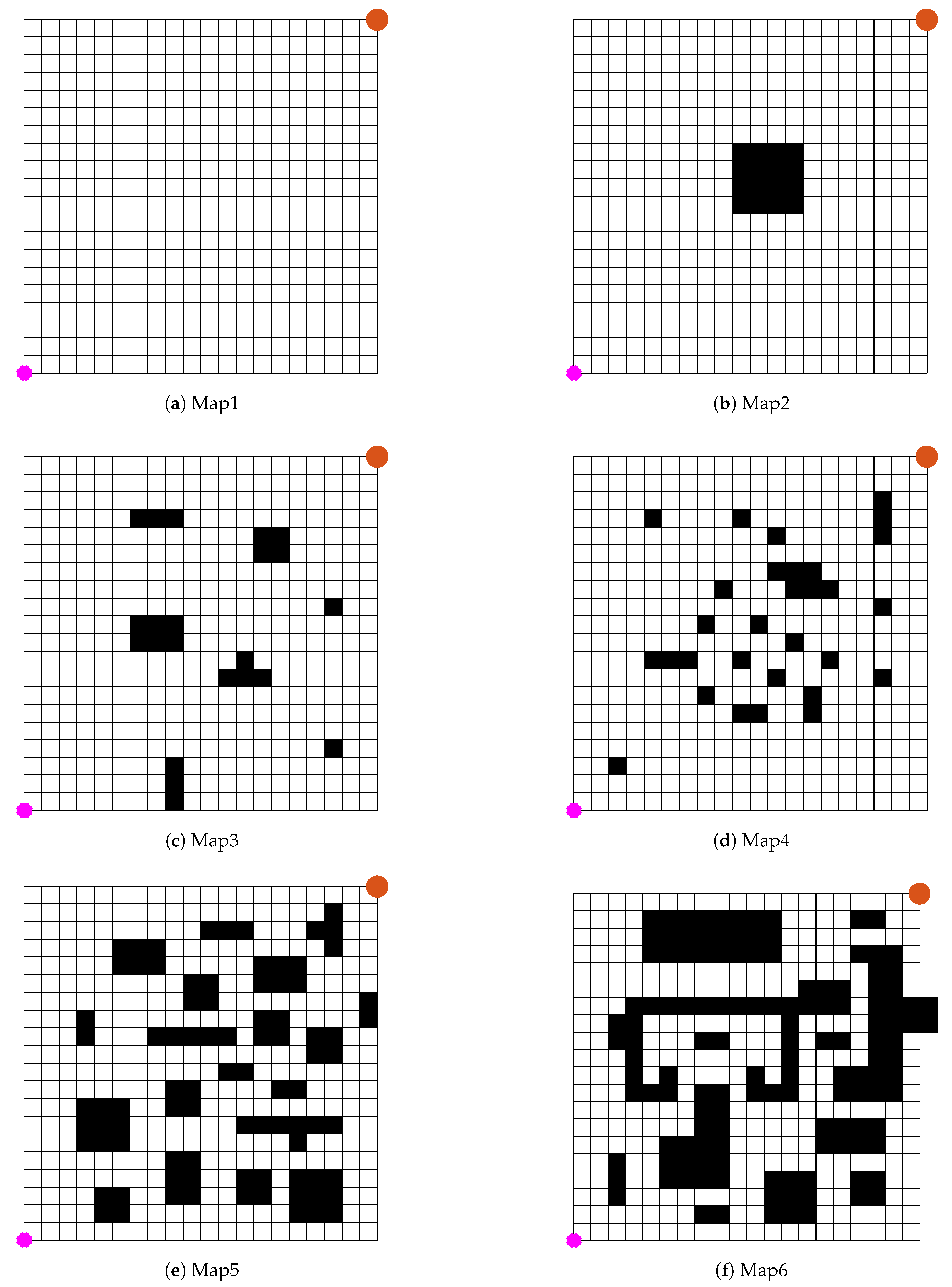
Figure 14.
The results of performing the pruning operation on the initial paths. The black paths are the initial paths and the red paths are the pruned paths.
Figure 14.
The results of performing the pruning operation on the initial paths. The black paths are the initial paths and the red paths are the pruned paths.
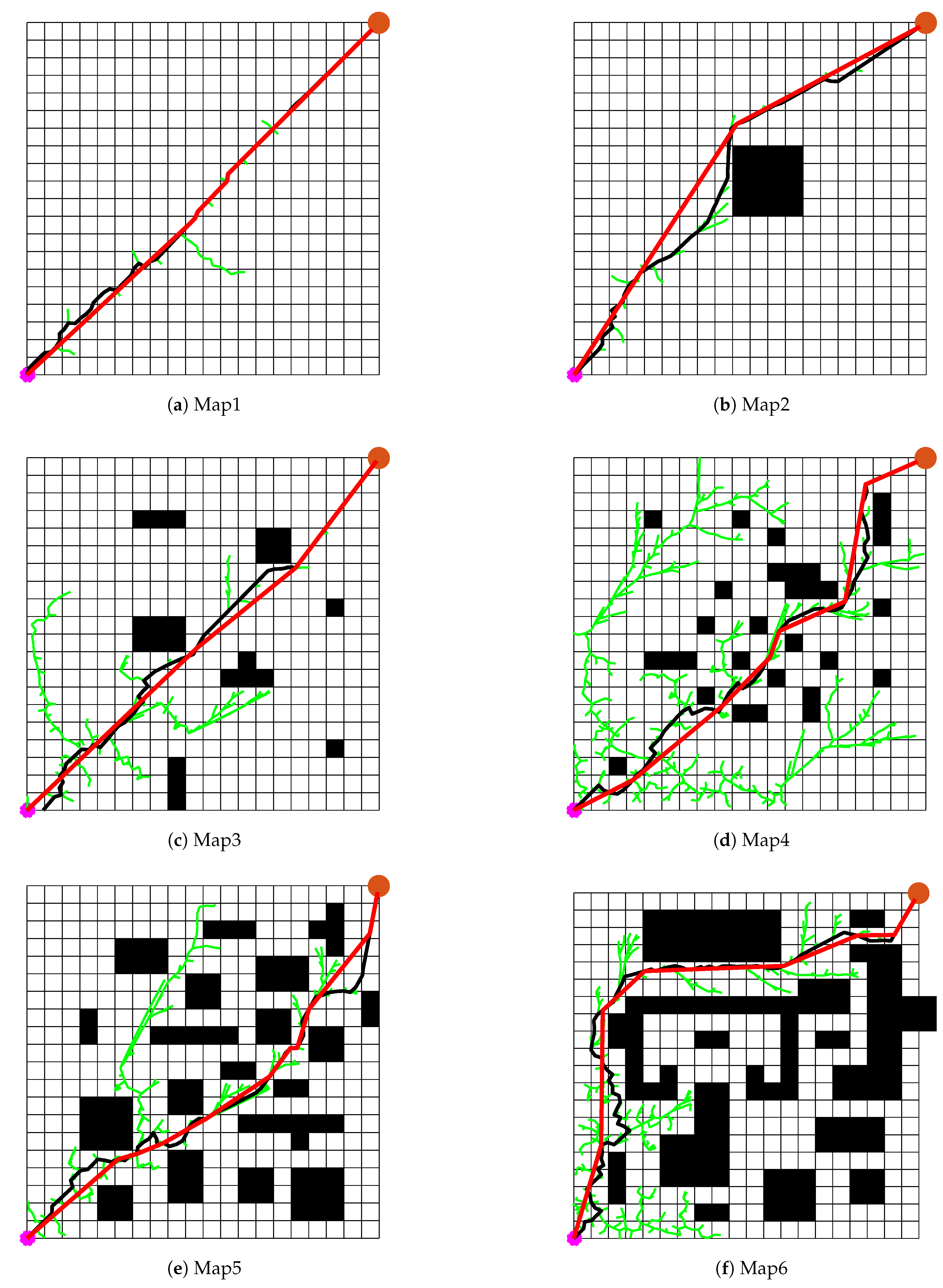
Figure 15.
3D urban map model
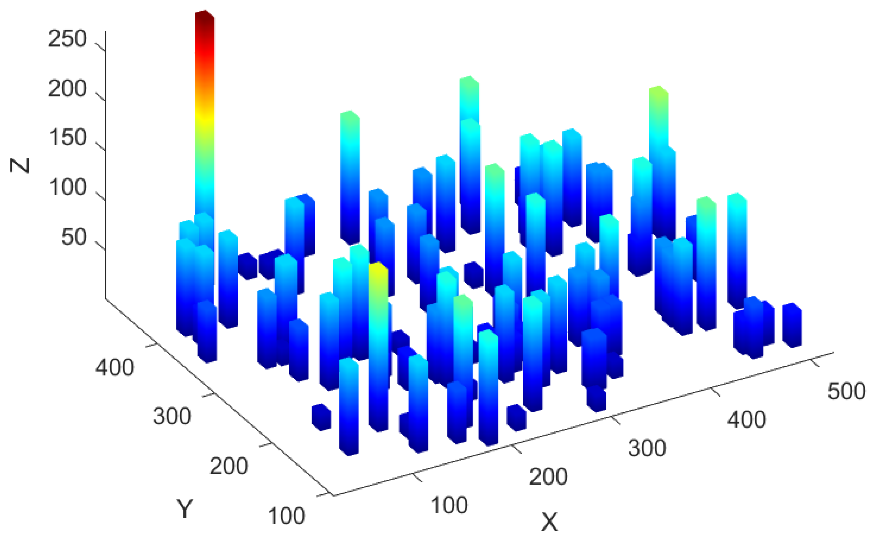
Figure 16.
Yaw angle and turning angle
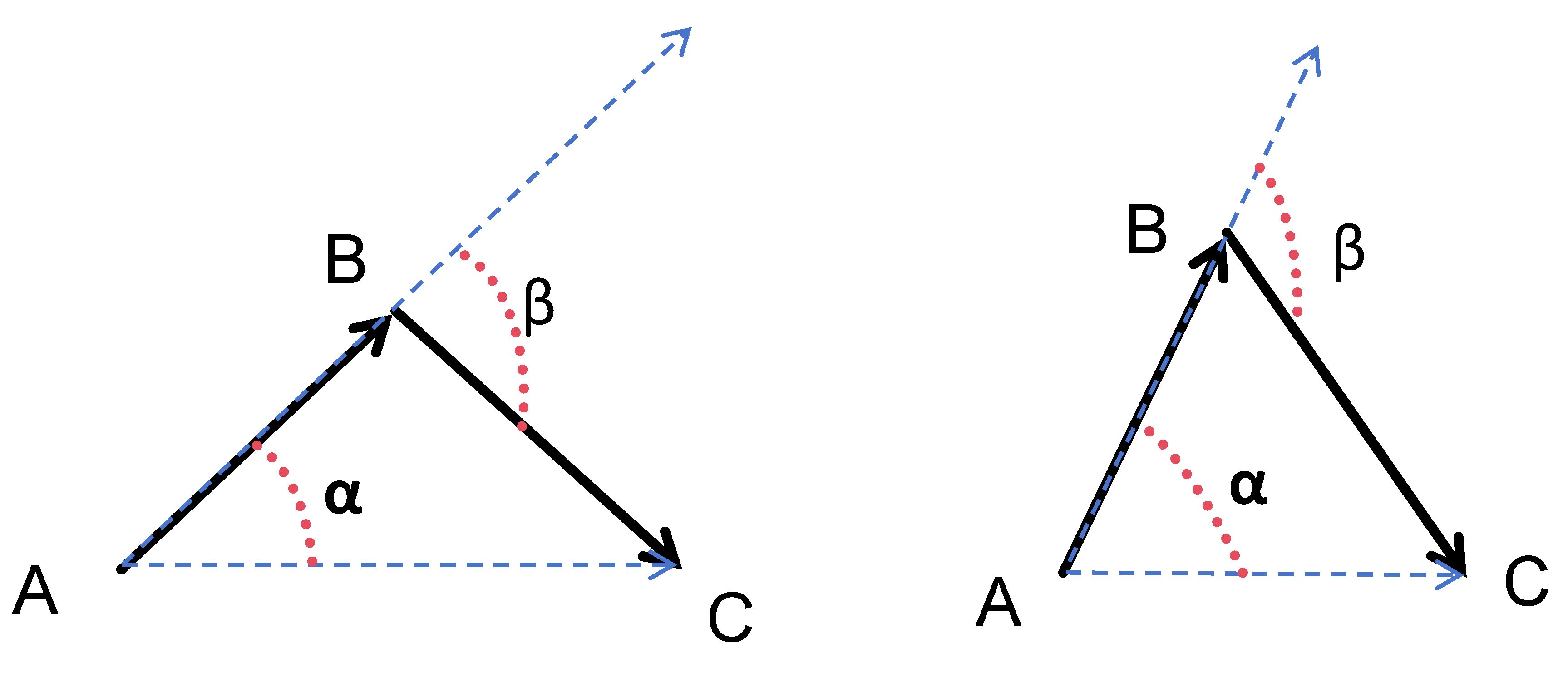
Figure 17.
Results of the algorithms in 3D urban path planning.
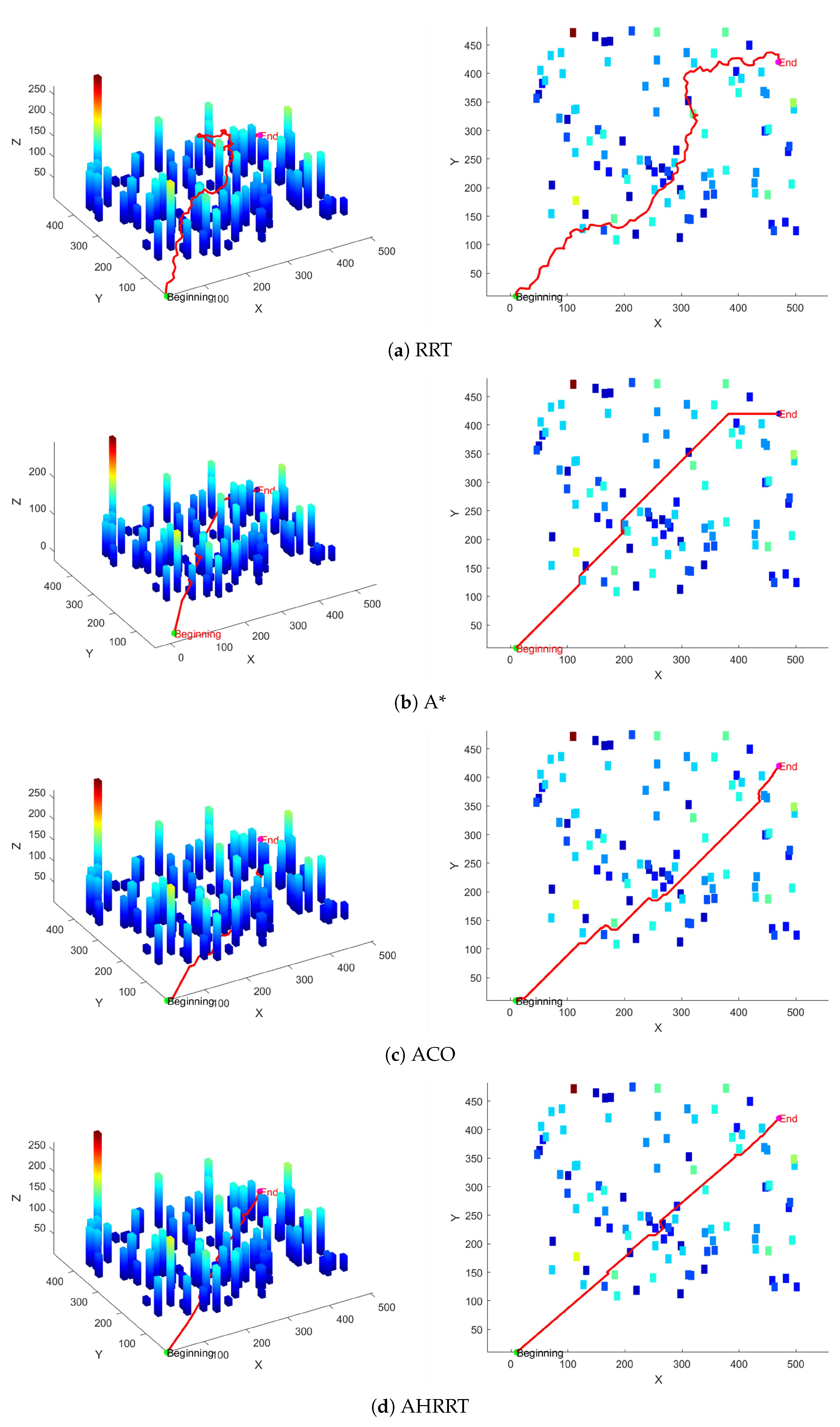
Table 2.
Length of the paths generated by the AHRRTs with different p values in different maps. indicates average length and indicates standard deviation.
Table 2.
Length of the paths generated by the AHRRTs with different p values in different maps. indicates average length and indicates standard deviation.
| Algorithm | Metrics | Map1 | Map2 | Map3 | Map4 | Map5 | Map6 |
|---|---|---|---|---|---|---|---|
| AHRRT(p=0.1) | Ave | 1465.01 | 1520.27 | 1507.44 | 1587.31 | 1599.22 | 1746.71 |
| Std | 17.81 | 26.01 | 47.41 | 47.55 | 70.92 | 59.88 | |
| AHRRT(p=0.3) | Ave | 1439.48 | 1497.58 | 1484.06 | 1572.13 | 1594.95 | 1737.38 |
| Std | 14.4 | 26.53 | 38.48 | 54.87 | 73.41 | 68.17 | |
| AHRRT(p=0.5) | Ave | 1421.17 | 1486.32 | 1471.2 | 1565.06 | 1581.54 | 1744.99 |
| Std | 8.49 | 25.90 | 42.78 | 48.04 | 64.76 | 65.55 | |
| AHRRT(p=0.7) | Ave | 1410.32 | 1477.1 | 1464.53 | 1551.73 | 1576.09 | 1739.62 |
| Std | 10.81 | 24.28 | 50.18 | 50.8 | 67.01 | 63.00 | |
| AHRRT(p=0.9) | Ave | 1400 | 1467.79 | 1453.55 | 1543.14 | 1581.63 | 1731.67 |
| Std | 0.00 | 25.02 | 40.50 | 52.22 | 69.57 | 57.61 |
Table 3.
Time consumption of the AHRRTs with different p values in different maps. indicates average time consumption and indicates standard deviation.
Table 3.
Time consumption of the AHRRTs with different p values in different maps. indicates average time consumption and indicates standard deviation.
| Algorithm | Metrics | Map1 | Map2 | Map3 | Map4 | Map5 | Map6 |
|---|---|---|---|---|---|---|---|
| AHRRT(p=0.1) | Ave | 0.0729 | 0.0498 | 0.0648 | 0.1748 | 0.4820 | 3.7059 |
| Std | 0.0204 | 0.0116 | 0.0233 | 0.1291 | 0.4008 | 2.2934 | |
| AHRRT(p=0.3) | Ave | 0.0319 | 0.0291 | 0.0398 | 0.1520 | 0.5363 | 4.0908 |
| Std | 0.0064 | 0.0070 | 0.0215 | 0.1745 | 0.5158 | 3.0325 | |
| AHRRT(p=0.5) | Ave | 0.0220 | 0.0288 | 0.0471 | 0.1863 | 0.6611 | 5.0896 |
| Std | 0.0038 | 0.0091 | 0.0334 | 0.1872 | 0.7286 | 3.2848 | |
| AHRRT(p=0.7) | Ave | 0.0180 | 0.0343 | 0.0677 | 0.4486 | 1.0869 | 9.6615 |
| Std | 0.0027 | 0.0125 | 0.0511 | 0.4750 | 1.1063 | 5.7035 | |
| AHRRT(p=0.9) | Ave | 0.0148 | 0.0850 | 0.1620 | 0.8494 | 2.8428 | 41.0255 |
| Std | 0.0021 | 0.0419 | 0.1093 | 1.3420 | 2.8847 | 25.3545 |
Table 4.
Waypoints of the AHRRTs with different p values in different maps. indicates average number of waypoints and indicates standard deviation.
Table 4.
Waypoints of the AHRRTs with different p values in different maps. indicates average number of waypoints and indicates standard deviation.
| Algorithm | Metrics | Map1 | Map2 | Map3 | Map4 | Map5 | Map6 |
|---|---|---|---|---|---|---|---|
| AHRRT(p=0.1) | Ave | 74.34 | 77.08 | 76.08 | 80.59 | 81.41 | 89.38 |
| Std | 0.92 | 1.29 | 2.01 | 2.43 | 3.62 | 3.23 | |
| AHRRT(p=0.3) | Ave | 73.00 | 75.92 | 75.26 | 79.92 | 81.10 | 88.86 |
| Std | 0.73 | 1.32 | 1.97 | 2.47 | 3.73 | 3.64 | |
| AHRRT(p=0.5) | Ave | 72.06 | 75.37 | 75.26 | 79.42 | 80.39 | 89.28 |
| Std | 0.42 | 1.31 | 2.58 | 2.45 | 3.32 | 3.52 | |
| AHRRT(p=0.7) | Ave | 71.46 | 74.89 | 74.66 | 78.76 | 80.06 | 89.10 |
| Std | 0.50 | 1.23 | 2.65 | 2.56 | 3.38 | 3.36 | |
| AHRRT(p=0.9) | Ave | 71.04 | 74.42 | 73.46 | 78.32 | 80.30 | 88.61 |
| Std | 0.20 | 1.26 | 2.02 | 2.67 | 3.57 | 3.05 |
Table 5.
Number of the nodes of the AHRRTs with different p values in different maps. indicates average number of nodes and indicates standard deviation.
Table 5.
Number of the nodes of the AHRRTs with different p values in different maps. indicates average number of nodes and indicates standard deviation.
| Algorithm | Metrics | Map1 | Map2 | Map3 | Map4 | Map5 | Map6 |
|---|---|---|---|---|---|---|---|
| AHRRT(p=0.1) | Ave | 236.38 | 218.51 | 332.90 | 805.96 | 1224.80 | 4536.44 |
| Std | 33.53 | 40.08 | 76.05 | 299.89 | 591.26 | 1399.15 | |
| AHRRT(p=0.3) | Ave | 133.32 | 340.68 | 256.88 | 822.55 | 1359.22 | 5668.88 |
| Std | 12.79 | 106.42 | 99.73 | 419.67 | 773.18 | 1927.48 | |
| AHRRT(p=0.5) | Ave | 100.34 | 238.35 | 287.27 | 1075.95 | 1787.42 | 7482.05 |
| Std | 6.35 | 65.95 | 148.65 | 542.75 | 1099.60 | 2528.79 | |
| AHRRT(p=0.7) | Ave | 84.14 | 315.38 | 409.77 | 1753.72 | 2936.88 | 13529.56 |
| Std | 4.49 | 105.85 | 242.40 | 871.24 | 1818.76 | 4066.22 | |
| AHRRT(p=0.9) | Ave | 73.68 | 810.76 | 974.92 | 4838.79 | 7997.73 | 39148.39 |
| Std | 2.16 | 344.93 | 549.43 | 3041.39 | 4725.41 | 12403.54 |
Table 6.
Length of the paths generated by the AHRRTs in different maps. indicates average length and indicates standard deviation.
Table 6.
Length of the paths generated by the AHRRTs in different maps. indicates average length and indicates standard deviation.
| Algorithm | Metrics | Map1 | Map2 | Map3 | Map4 | Map5 | Map6 |
|---|---|---|---|---|---|---|---|
| AHRRT1 | Ave | 1422.8 | 1502.4 | 1581.2 | 1602.8 | 1646 | 1834 |
| Std | 11.44 | 17.44 | 90.12 | 55.55 | 84.1 | 54.55 | |
| AHRRT2 | Ave | 1532.14 | 1592.46 | 1573.23 | 1659.31 | 1656.18 | 1871.78 |
| Std | 33.84 | 37.53 | 59.35 | 63.84 | 86.71 | 67.74 | |
| AHRRT3 | Ave | 1482.58 | 1636.82 | 1571.46 | 1746.98 | 1780.63 | 2119.26 |
| Std | 27.14 | 72.56 | 75.56 | 86.83 | 124.56 | 166.79 | |
| AHRRT | Ave | 1420.74 | 1501.75 | 1497.15 | 1598.13 | 1619.4 | 1805.28 |
| Std | 10.04 | 14.34 | 45.48 | 51.88 | 95.27 | 51.9 |
Table 7.
Time consumption of the AHRRTs in different maps. indicates average time consumption and indicates standard deviation.
Table 7.
Time consumption of the AHRRTs in different maps. indicates average time consumption and indicates standard deviation.
| Algorithm | Metrics | Map1 | Map2 | Map3 | Map4 | Map5 | Map6 |
|---|---|---|---|---|---|---|---|
| AHRRT1 | Ave | 0.0142 | 0.0517 | 0.7585 | 0.91 | 2.573 | 12.6449 |
| Std | 0.0026 | 0.0234 | 0.6353 | 0.7324 | 1.972 | 6.9629 | |
| AHRRT2 | Ave | 10.2572 | 5.5755 | 6.4762 | 6.2088 | 9.7978 | 14.032 |
| Std | 9.7467 | 5.6788 | 6.177 | 5.6784 | 7.325 | 5.3086 | |
| AHRRT3 | Ave | 0.022 | 0.0538 | 0.1199 | 0.7247 | 1.4506 | 3.9229 |
| Std | 0.0032 | 0.0215 | 0.1395 | 0.7437 | 1.3478 | 1.9771 | |
| AHRRT | Ave | 0.0138 | 0.0313 | 0.0665 | 0.712 | 2.0138 | 8.586 |
| Std | 0.00124 | 0.0170 | 0.0433 | 0.6732 | 1.228 | 4.8756 |
Table 8.
Waypoints of the AHRRTs in different maps. indicates average number of waypoints and indicates standard deviation.
Table 8.
Waypoints of the AHRRTs in different maps. indicates average number of waypoints and indicates standard deviation.
| Algorithm | Metrics | Map1 | Map2 | Map3 | Map4 | Map5 | Map6 |
|---|---|---|---|---|---|---|---|
| AHRRT1 | Ave | 72.14 | 76.12 | 80.06 | 81.14 | 83.30 | 92.70 |
| Std | 0.57 | 0.87 | 4.51 | 2.78 | 4.21 | 2.73 | |
| AHRRT2 | Ave | 78.38 | 81.46 | 80.70 | 85.02 | 85.00 | 97.02 |
| Std | 2.04 | 2.10 | 3.05 | 3.39 | 4.52 | 3.70 | |
| AHRRT3 | Ave | 75.16 | 82.88 | 79.64 | 88.44 | 90.18 | 107.48 |
| Std | 1.36 | 3.61 | 3.85 | 4.35 | 6.27 | 8.33 | |
| AHRRT | Ave | 72.06 | 76.42 | 75.92 | 81.34 | 82.38 | 93.74 |
| Std | 0.51 | 1.20 | 2.28 | 2.72 | 4.76 | 2.83 |
Table 9.
Number of the nodes of the AHRRTs in different maps. indicates average number of nodes and indicates standard deviation.
Table 9.
Number of the nodes of the AHRRTs in different maps. indicates average number of nodes and indicates standard deviation.
| Algorithm | Metrics | Map1 | Map2 | Map3 | Map4 | Map5 | Map6 |
|---|---|---|---|---|---|---|---|
| AHRRT1 | Ave | 98.46 | 254.44 | 451.78 | 1940.74 | 2951.76 | 12465.86 |
| Std | 6.22 | 58.97 | 371.86 | 875.53 | 1238.4 | 2735.38 | |
| AHRRT2 | Ave | 2291.6 | 2558.98 | 2519.32 | 3426.3 | 3716.14 | 8804.16 |
| Std | 1093.67 | 1250.15 | 1249.16 | 1249.27 | 1279.33 | 1593.53 | |
| AHRRT3 | Ave | 106.14 | 252.92 | 291.88 | 1192.62 | 1675.52 | 5572.66 |
| Std | 8.48 | 72.55 | 186.95 | 651.67 | 947.14 | 1731.14 | |
| AHRRT | Ave | 100.84 | 266.78 | 308.16 | 1918.96 | 1802.66 | 5958.64 |
| Std | 6.94 | 62.35 | 121.36 | 872.77 | 1056.3 | 1408.04 |
| Algorithm | Parameter | Value |
|---|---|---|
| ACO | Maximum iterations T | 100 |
| Pheromone evaporation coefficient | 0.3 | |
| Population N | 50 | |
| A* | Heuristic weight | 1 |
| Stepsize | 26 | |
| RRT | Stepsize | 5 |
| AHRRT | Stepsize | 5 |
| Target bias probability p | 0.5 |
Table 13.
The path planning results of AHRRT and other algorithms.
| Metrics | RRT | A* | ACO | AHRRT |
|---|---|---|---|---|
| t(s) | 0.07971 | 18.417 | 0.2643 | 0.01468 |
| l(m) | 997.3509 | 738.0945 | 667.6615 | 659.5079 |
| w | 104.16 | 538.33 | 550.67 | 93.87 |
| m | 13199.23 | 272511 | 14300 | 887.6 |
| 98.02% | 64.18% | 90% | 100% | |
| () | 97.9821 | 109.4712 | 173.6598 | 102.7654 |
| n(times) | 50.68 | 91 | 49 | 11.23 |
Disclaimer/Publisher’s Note: The statements, opinions and data contained in all publications are solely those of the individual author(s) and contributor(s) and not of MDPI and/or the editor(s). MDPI and/or the editor(s) disclaim responsibility for any injury to people or property resulting from any ideas, methods, instructions or products referred to in the content. |
© 2025 by the authors. Licensee MDPI, Basel, Switzerland. This article is an open access article distributed under the terms and conditions of the Creative Commons Attribution (CC BY) license (http://creativecommons.org/licenses/by/4.0/).
Copyright: This open access article is published under a Creative Commons CC BY 4.0 license, which permit the free download, distribution, and reuse, provided that the author and preprint are cited in any reuse.


