U(1)-Driven Local Holographic Screens (Horizons): Holographic Bit–Mode Balance and the α-Fixpoint

1. Introduction and Motivation

A central lesson of holographic thinking is that the number of physically accessible degrees of freedom in a gravitating region scales not with its volume, but with an associated boundary or horizon area. Black-hole thermodynamics makes this explicit through the entropy–area relation, and modern quantum-informational approaches refine it into a sharp statement: a geometrically fixed upper bound exists on the amount of independent classical information (bits) that can be stored on a horizon assigned to a given region [1,2,3,5,6,7].

In parallel, the fine-structure constant $\alpha$ is known with extraordinary precision and, within observational bounds, appears strikingly stable across space and time [8,9]. Yet in the Standard Model it remains a free dimensionless parameter. Its unit-independence and robustness strongly suggest that $\alpha$ may be fixed by a geometric and information-based mechanism rather than by contingent microphysics alone [17].

My previous work approached this question from two complementary directions. First, I showed that $\alpha$ can naturally emerge from a holographic bit–mode equilibrium [18]: at an appropriately selected horizon scale, the maximal bit capacity implied by area information bounds matches the number of electromagnetic degrees of freedom, producing $\alpha$ as an output. Second, in quantized-horizon settings [19] I explored how physically relevant effective quantities become boundary- or horizon-neighborhood objects rather than volume averages, emphasizing the operational role of horizons in organizing accessible states. These results point to a shared theme: horizon information constraints are not merely global but may also be physically meaningful in local contexts .

The present paper develops this idea into a systematic local mechanism. Our guiding question is:

Can there exist a local, quantized horizon whose radius is not arbitrary but is selected as a fixed point of balance between the local $U\left(1\right)$ mode demand and a holographic bit-capacity bound, and such that evaluating natural dimensionless electromagnetic ratios on that fixed point yields the observed fine-structure constant α?

We answer in the affirmative by introducing the Holographic Bit–Mode Balance (HBMB) principle. In a locally defined region of radius R, two independent quantities compete. The first is the horizon bit capacity $S_{\mathrm{bit}}\left(R\right)$ implied by a local area-law bound and quantized at the Planck scale. The second is the number of redundancy-free, physically occupiable $U\left(1\right)$ eigenmodes $N_{U\left(1\right)\mathrm{mode}}(R;\mathcal{B})$, determined by local boundary data $\mathcal{B}$ (impedances, material response, spectral window, etc.). HBMB asserts that $U\left(1\right)$ mode realization is capped by the boundary information capacity. The stable realized state sits at a radius $R_{*}$ where

$$S_{\mathrm{bit}}\left(R_{*}\right)=N_{U\left(1\right)\mathrm{mode}}(R_{*};\mathcal{B}),$$

(1)

and this fixed point is locally stable against small perturbations in R.

The main claim of this paper is that the HBMB fixed point simultaneously defines an $\alpha$-fixpoint: at the stabilized local holographic screen (horizon) $R_{*}$, natural dimensionless electromagnetic combinations—in particular the ratio of the vacuum impedance $Z_0$ to the quantum Hall resistance scale (von Klitzing constant) $R_K$—return the measured fine-structure constant [24]. Crucially, $\alpha$ enters neither the definition of $S_{\mathrm{bit}}$ nor that of $N_{U\left(1\right)\mathrm{mode}}$; it appears solely as an output after stabilization. The spatiotemporal constancy of $\alpha$ is then a consequence of the robustness of the HBMB attractor, as long as the local $U\left(1\right)$ environment and the quantized horizon structure are not dramatically altered.

We now outline the boundary-physics ingredients that motivate HBMB and make local holographic horizons natural.

1.1. Boundary Degrees of Freedom in $U\left(1\right)$ Gauge Theories (Edge Modes)

In $U\left(1\right)$ gauge theories, the raw counting of bulk modes is not physical: gauge redundancy identifies many mathematical configurations as the same physical state. When a region is defined by cutting space with a boundary, part of the gauge structure cannot be eliminated purely by bulk constraints. Instead, additional, physically relevant degrees of freedom appear on the boundary. These are the edge modes. For Maxwell theory they resolve the long-standing contact-term puzzle in entanglement entropy and provide an explicit statistical interpretation: edge modes are classical solutions labeled by boundary electric flux that contribute a genuine boundary entropy [10,11].

Operationally, $U\left(1\right)$ edge modes therefore encode the information capacity associated with a local cut. They quantify how many distinct, physically distinguishable $U\left(1\right)$ configurations within a region can become classically accessible. This boundary information viewpoint is essential for treating a local holographic screen (horizon) not as a passive geometric surface but as an information-limiting object constraining realizable states.

1.2. Horizon as a Physical Boundary: Membrane/Impedance and Soft Hair

Figure 1. Fluctuation-driven (current-source/Norton) impedance-divider model used to interpret the accessible edge fraction as a dissipated fraction on the local holographic screen (horizon). This motivates $F_{U\left(1\right)}\simeq Z_{\mathrm{surf}}/(Z_{\mathrm{surf}}+Z_{\mathrm{int}})$ with $Z_{\mathrm{int}}\sim R_K/k$.

Figure 1. Fluctuation-driven (current-source/Norton) impedance-divider model used to interpret the accessible edge fraction as a dissipated fraction on the local holographic screen (horizon). This motivates $F_{U\left(1\right)}\simeq Z_{\mathrm{surf}}/(Z_{\mathrm{surf}}+Z_{\mathrm{int}})$ with $Z_{\mathrm{int}}\sim R_K/k$.

Modern horizon physics reinforces that boundaries are dynamical. In the membrane paradigm, a (local) horizon behaves effectively like a physical surface endowed with electromagnetic response: surface currents and dissipative boundary conditions encode the interaction of fields with the horizon. A key operational imprint is that the horizon’s surface resistivity is of order the vacuum impedance, linking horizon electrodynamics directly to $Z_0$ [12].

Complementarily, soft-hair perspectives show that horizons carry nontrivial boundary charges and “soft” $U\left(1\right)$ configurations tied to large gauge transformations. For black holes, soft photon hair represents $U\left(1\right)$ degrees of freedom living on the horizon and storing information on a holographic plate [13]. Thus, from the $U\left(1\right)$ standpoint, horizons are active boundaries that both constrain and encode the physically realizable configuration space. HBMB formalizes precisely this interplay: local $U\left(1\right)$ mode demand is regulated by boundary capacity.

1.3. Why a Universal Dimensionless Ratio Is Expected

If two independent principles—(i) the redundancy-free $U\left(1\right)$ mode count admitted by the local environment and (ii) the holographic bit capacity implied by a local area-law bound—are forced into equality at a stable fixed point, then any natural electromagnetic ratios evaluated there must be dimensionless and universal. The HBMB fixed point is not a tuned scale; $R_{*}$ follows entirely from measurable local boundary data and the area-law information bound. Consequently, $\alpha$ emerges not as numerology but as the scheme-independent imprint of a stable information-theoretic attractor set by $U\left(1\right)$ boundary physics and holography.

In the broader context of horizon thermodynamics, it is worth emphasizing that the use of local (operationally defined) horizons is not ad hoc. A classic motivation comes from Jacobson’s observation that, under suitable assumptions, imposing a local entropy–energy balance for local Rindler horizons can be viewed as an “equation of state” perspective on gravity [4]. The present work does not attempt to derive Einstein dynamics; rather, we use the same guiding philosophy to test whether the HBMB local-horizon balance is compatible with known QFT modular-energy structure and with the geometric focusing logic that underlies horizon thermodynamics.

1.4. Novelty and Key Contributions

Because editors and referees often judge submissions from the abstract, introduction, and conclusion alone, we state here what is new and what is not claimed.

• Operational observable: we define a dimensionless accessibility fraction

  $$F_{U\left(1\right)}=S_{\mathrm{edge},\mathrm{acc}}/S_{\mathrm{edge},\mathrm{total}}$$

  that quantifies the portion of $U\left(1\right)$ edge configurations that remain redundancy-free under local boundary data.
• Explicit matching (not a postulate): we compute $F_{U\left(1\right)}$ at the HBMB fixed point from a fluctuation-driven (current-source) impedance-divider model of dissipation, obtaining $F_{U\left(1\right)}\left(R^{★}\right)\simeq Z_0/(Z_0+2R_K)=\alpha +\mathcal{O}\left({\alpha }^2\right)$.
• First-principles impedance scale: using linear response (Kubo) and the universal quantum resistance scale, we motivate $Z_{\mathrm{int}}\sim R_K$ up to a dimensionless normalisation factor; the “2” follows the standard QED convention behind $\alpha =Z_0/\left(2R_K\right)$.
• Robust scale selection: we motivate why $R^{★}$ is set by the Compton-scale driving frequency and verify robustness against higher multipoles (TM $\ell =2$) and a short TE check.
• Controlled consistency checks: we show (i) UV-divergent terms cancel in the ratio defining $F_{U\left(1\right)}$, and (ii) the modular-energy scaling on the QFT side matches the $R^4$ focusing scaling on the geometric side in a weak-focusing regime.
• Scope and limitations: the construction is a consistency and falsifiability framework; it does not derive the full Einstein equations nor the full QED $\beta$-function.

In the next sections we formalize the HBMB principle, prove fixed-point existence and stability, and derive falsifiable plateau–jump phenomenology implied by the quantized bit–mode structure.

2. Related Work and Background

This section summarizes the theoretical lines that connect most directly to (i) locally interpreted holographic horizons and area-law information bounds, (ii) existing approaches to the origin of the fine-structure constant $\alpha$, and (iii) $U\left(1\right)$ configuration-space constructions that resemble holographic reasoning. The aim is not a full literature review, but a focused positioning of the present work within three background pillars, and then within my own already published results.

2.1. Holographic Entropy and an Upper Bound on Bits

The holographic principle historically emerged from black-hole thermodynamics and the entropy–area relation. In its canonical form, the maximal entropy that a gravitating region can store scales with an associated boundary or horizon area rather than with its volume [1,2,3]. In natural units this area law reads

$$S_{max}\left(R\right)={\displaystyle \frac{A\left(R\right)}{4{\ell }_P^2}},$$

(2)

where $A\left(R\right)$ is the boundary area for a region of characteristic radius R (for a sphere $A=4\pi R^2$) and ${\ell }_P$ is the Planck length. Hence, for a spherical surface one has

$$S_{max}\left(R\right)=\pi {\left({\displaystyle \frac{R}{{\ell }_P}}\right)}^2.$$

(3)

Moreover, in the AdS limit where standard holography is sharply defined, we show in a companion work that HBMB “eigensynthesis” reproduces the HKLL bulk reconstruction (smearing) map to machine precision, supporting the view that HBMB is not foreign to established AdS/CFT reconstruction but rather extends the same logic to local holographic screens (horizons) where a global boundary description is absent [20,21].

When one wishes to measure information explicitly in bits rather than in natural-log units, the conversion introduces a factor $ln2$:

$$S_{\mathrm{bit}}\left(R\right)={\displaystyle \frac{S_{max}\left(R\right)}{ln2}}={\displaystyle \frac{A\left(R\right)}{4{\ell }_P^{2}ln2}}.$$

(4)

Operationally, $S_{\mathrm{bit}}\left(R\right)$ is the maximal number of independent classical records that can be stored on the boundary/horizon.

To address the common concern that ${\ell }_P$ “belongs” only to gravitational systems, Appendix C provides an explicit QFT+geometry consistency check (modular energy in a ball and Raychaudhuri focusing) showing how ${\ell }_P^2$ enters as the universal entropy-density conversion scale in the local entropy-balance route.

Different formulations of holography—Bekenstein–Hawking entropy, QFT in curved spacetime with UV cutoffs, and modern quantum-informational treatments of entanglement entropy—all converge on the same message: the accessible state-space capacity of a region cannot be increased arbitrarily; a geometric boundary provides a hard upper constraint [1,2,3].

In this paper we adopt a local reading of the area law. We do not assume a global cosmological horizon, but rather a physically relevant, locally defined spatial domain bounded by a closed surface. To that surface we attach $S_{max}\left(R\right)$ (or in bit units $S_{\mathrm{bit}}\left(R\right)$), and compare it with the number of locally realizable electromagnetic $U\left(1\right)$ modes. A key conceptual point is that area scaling does not imply that the underlying dynamics inside the region becomes two-dimensional. Instead, it states that the upper bound on classically accessible information is controlled by a two-dimensional geometric quantity, the boundary area. The electromagnetic modes still live in a three-dimensional volume. The $U\left(1\right)$ symmetry is an internal (gauge) symmetry of the field phase space, not a statement about spatial dimensionality; therefore there is no tension between 3D bulk field dynamics and a 2D area-controlled information bound.

2.2. On the Origin of the Fine-Structure Constant

The fine-structure constant $\alpha \approx 1/137.036$ is the central dimensionless coupling of quantum electrodynamics. In its standard form it measures the strength of electromagnetic interaction:

$$\alpha ={\displaystyle \frac{e^2}{4\pi {\epsilon }_0\hslash c}},$$

(5)

with e the elementary charge, ${\epsilon }_0$ the vacuum permittivity, ℏ Planck’s constant, and c the speed of light. In the Standard Model $\alpha$ is an input parameter; no internal mechanism fixes its numerical value or explains its remarkable spatiotemporal stability. Precisely this stability and dimensionless nature suggest that $\alpha$ may be fixed by a geometric or information-theoretic attractor [17].

A wide spectrum of ideas has been proposed for deriving $\alpha$ from first principles, ranging from dimensional-analysis constructions built from fundamental constants, to grand-unification and running-coupling perspectives, and to closed-form numerical approximations based on special numbers (such as $\pi$, e, zeta-values, etc.). These approaches typically suffer from strong model dependence, sensitivity to regularization/normalization choices, or lack a clear physical principle that selects the relevant scale where $\alpha$ should be evaluated.

A long-known but often treated as a metrological identity rewrites $\alpha$ as a purely electromagnetic impedance ratio:

$$\alpha ={\displaystyle \frac{Z_0}{2R_K}},$$

(6)

where $Z_0=\sqrt{{\mu }_0/{\epsilon }_0}\simeq 377\Omega$ is the vacuum impedance and $R_K=h/e^2\simeq 25.8\mathrm{k}\Omega$ is the von Klitzing constant of the quantum Hall effect. This form strongly hints that $\alpha$ measures a ratio between a classical vacuum boundary response ($Z_0$) and a universal quantum-transport scale ($R_K$). However, by itself it is not yet an explanation: one still needs a physical mechanism that selects the local boundary/horizon scale where such a ratio becomes a stable fixed point. The HBMB framework introduced here supplies precisely this missing step, by interpreting $\alpha$ not as an assumed normalization, but as a consequence of a local holographic bit–mode equilibrium.

2.3. $U\left(1\right)$ Configuration-Space Geometry and “bare $\alpha$”

A partially independent but thematically related direction aims to derive $\alpha$ from the geometry of $U\left(1\right)$ configuration space. In these constructions the space of physical configurations (gauge-equivalence classes) is embedded into a compact higher-dimensional domain, and a dimensionless coupling is defined as a measure ratio between an “interior” region and its boundary. This yields a closed-form “bare $\alpha$” which is then related to the experimental value via QED dressing.

The conceptual value of this line lies in showing that a $U\left(1\right)$ symmetry combined with a compact configuration space can naturally generate dimensionless couplings, and that interior-to-boundary projection plays a central role—an intuition closely aligned with holography [22]. Technically, however, the outcome is strongly choice-dependent: it is sensitive to the configuration-space measure and metric, the normalization chosen for the boundary projection, and the specific way interior and boundary quantities are combined into a dimensionless coupling. Consequently, the numerical result is not scheme-independent. The present work differs in that normalization is not a free choice: it is fixed by a local equilibrium (HBMB) attractor, hence has an operational physical status.

2.4. My Earlier Results on Quantized Horizons, HBMB, and $\alpha$

The current paper should be viewed as a local synthesis of two already published lines. First, in my work on quantized horizons and holographic vacuum energy, I argued that when horizon information capacity is quantized at the Planck scale, physically relevant effective quantities acquire their scale not from bulk volume averages but from an operationally selected horizon-neighborhood domain [19]. This provides motivation to treat horizons as information-organizing boundaries also in a local sense.

Second, the direct predecessor is my holographic derivation of $\alpha$ via the Holographic Bit–Mode Balance (HBMB) principle [18]. There I compared the maximal surface-bit capacity of a local micro-horizon,

$$S_{max}=\pi {\left({\displaystyle \frac{R_e}{{\ell }_P}}\right)}^2,$$

(7)

to the total redundancy-free degeneracy of interior Dirac-field modes under MIT boundary conditions. The latter decomposes into four nested contributions: (i) the base degeneracy of the lowest Dirac modes $g_{\mathrm{geom}}$, (ii) a curvature-sensitive logarithmic Seeley–DeWitt correction $g_{log}$, and (iii) a uniform-WKB, zeta-regularized high-ℓ tail $g_{\mathrm{tail}}$ capturing large-angular-momentum, boundary-grazing modes. Their sum yields $g_{\mathrm{tot}}=g_{\mathrm{geom}}+g_{log}+g_{\mathrm{tail}}$, and the fixed-point ratio

$${\alpha }^{-1}={\displaystyle \frac{S_{max}}{g_{\mathrm{tot}}}}=137.035998\left(20\right),$$

(8)

reproducing the observed value within uncertainties [18].

It is important to note that while the micro-horizon radius $R_e$ (or the associated local-horizon scale) was already derived and physically motivated there, it could still appear partly hypothetical to the reader. The present work makes this point strict: the local holographic screen (horizon) radius is not an assumed input, but emerges as the HBMB fixed point set by the equality between the redundancy-free $U\left(1\right)$ mode count and the area-law bit capacity. Therefore $R_{*}$ is operationally definable from measurable local $U\left(1\right)$ boundary data, and the micro-scale used in the previous $\alpha$ derivation gains a substantially stronger physical status through the $U\left(1\right)$–holography balance mechanism developed here.

With this background established, the next section fixes the necessary definitions and notation: the local quantized horizon and its fixed-point radius $R_{*}$, the precise surface-bit capacity $S_{max}\left(R\right)$ (and $S_{\mathrm{bit}}\left(R\right)$), the effective redundancy-free $U\left(1\right)$ mode number $N_{\mathrm{mode}}^{U\left(1\right)}(R;\mathcal{B})$, and the local electromagnetic boundary/environment parameter package $\mathcal{B}$. These provide the formal basis for the HBMB mechanism and the derivation of the $\alpha$-fixpoint.

3. Core Definitions and Notation: Local Quantized Horizon and HBMB

This section fixes the formal framework of the paper. We will compare two quantities defined on a locally selected spatial domain: (i) the maximal classical information capacity (bit capacity) allowed by the boundary/horizon, and (ii) the redundancy-free number of physically realizable electromagnetic $U\left(1\right)$ modes within that domain. The Holographic Bit–Mode Balance (HBMB) principle states that these two quantities equalize at a stable fixed point, which dynamically selects the radius of the local horizon.

3.1. Local Quantized Horizon (Definition)

By a local quantized horizon we mean a closed, physically relevant boundary surface $\Sigma \left(R\right)$ that encloses a region of characteristic radius R, and to which a local reading of the holographic area law assigns a maximal information capacity. The adjective “local” emphasizes that we are not invoking a global cosmological event horizon, but rather an operationally chosen domain boundary. The adjective “quantized” indicates that this capacity is naturally measured in Planck-scale bits, so that changes in the boundary area correspond to discrete information steps.

Definition 1 (Local holographic horizon / local screen). Fix an event p, a local timelike direction $u^a$ (the “rest frame” of the local description), and a characteristic scale R that delimits the regime of validity of the effective description. A local holographic horizon at scale R is an operationally defined “screen” $\Sigma \left(R\right)$ that acts as a one-way information boundary for the selected domain and for which (i) a horizon-thermodynamic entropy assignment is meaningful,

$$S_{\mathrm{BH}}\left(R\right)={\displaystyle \frac{A\left(R\right)}{4{\ell }_P^2}},$$

(9)

and (ii) a local energy/flux balance can be posed (in the sense of horizon thermodynamics or a stretched-horizon membrane description). Concretely, $\Sigma \left(R\right)$ may be taken as a near-zero-expansion null surface through p (a local Rindler-type construction) or as a regulated stretched version thereof; we emphasize that this is not a global event horizon but a locally selected holographic screen.

Remark (realizations and robustness). The same operational notion admits several standard realizations: (i) a local Rindler horizon generated by a null congruence with $\theta \left(p\right)=0$ in the chosen frame, (ii) the boundary of a small causal diamond / entanglement ball of radius R used to define modular flow, or (iii) a stretched horizon in the membrane paradigm, where the screen is treated as an effective dissipative system with well-defined response coefficients. In this paper the choice of realization is used to formulate and test the HBMB entropy–reconstruction balance; it is not used to derive full gravitational dynamics.

Remark (nested screens and no double counting). Local holographic screens (horizons) at different scales should not be viewed as independent entropy budgets: smaller screens are overlapping subcodes of larger ones, so their capacities are non-additive; this naturally avoids double counting in multi-scale constructions (see Section 8). For transparency, we take the horizon geometry to be spherical in the first pass, so that $\Sigma \left(R\right)$ is an R-sphere with area $A\left(R\right)=4\pi R^2$. None of the later conclusions rely on spherical symmetry itself; the sphere merely provides the cleanest model for scale selection under an area-controlled capacity.

3.2. Holographic Bit Capacity

We define the local holographic screen (horizon) information capacity by the local area law. In entropy units (natural-log units) the maximal capacity reads [1,2,3]

$$S_{max}\left(R\right)={\displaystyle \frac{A\left(R\right)}{4{\ell }_P^2}}.$$

(10)

For a spherical surface this becomes

$$S_{max}\left(R\right)=\pi {\left({\displaystyle \frac{R}{{\ell }_P}}\right)}^2.$$

(11)

When the capacity is measured explicitly in bits, one divides by $ln2$:

$$S_{\mathrm{bit}}\left(R\right)={\displaystyle \frac{S_{max}\left(R\right)}{ln2}}={\displaystyle \frac{A\left(R\right)}{4{\ell }_P^{2}ln2}}.$$

(12)

Operationally, $S_{\mathrm{bit}}\left(R\right)$ is the maximal number of independent classical records that can be made accessible on the boundary.

A conceptual clarification is important here. Area scaling does not claim that the bulk field dynamics becomes two-dimensional. Rather, it asserts that the upper bound on classically accessible information is controlled by a two-dimensional geometric quantity, the boundary area. Electromagnetic modes still live in a three-dimensional volume; holography constrains how many of them can become simultaneously classical and distinguishable.

3.3. $U\left(1\right)$ Mode Demand and Redundancy-Free Mode Number

The second core quantity is the number of physically realizable degrees of freedom of the electromagnetic $U\left(1\right)$ field in the local region. In gauge theories raw mode counts are not physical because gauge redundancy identifies many mathematical configurations as the same state. When space is cut by a boundary, part of the gauge structure cannot be eliminated purely by bulk constraints, and physically relevant boundary data (edge degrees of freedom) appear [10,11]. Accordingly, the meaningful quantity is not the naive mode number but the redundancy-free count of distinct, occupiable modes compatible with local boundary data.

We denote this by

$$N_{\mathrm{mode}}^{U\left(1\right)}(R;\mathcal{B}),$$

(13)

where $\mathcal{B}$ is a local boundary/environment package encoding, for example: the effective boundary impedance or material response, the relevant spectral window, geometric cutoffs and UV regularization scales, and any other experimentally fixed data that determine the physical $U\left(1\right)$ spectrum in the region. Crucially, $\mathcal{B}$ is not a fitting freedom; it represents measurable or operationally specified properties of the local electromagnetic environment.

3.4. HBMB Principle and Fixed Point

Figure 2. Illustration of the leading-order accessibility/dissipation fraction $F_{U\left(1\right)}\approx Z_{\mathrm{surf}}/(Z_{\mathrm{surf}}+2R_K)$ as a function of the effective screen impedance. The canonical choice $Z_{\mathrm{surf}}=Z_0$ yields $F\simeq \alpha /(1+\alpha )=\alpha +\mathcal{O}\left({\alpha }^2\right)$.

Figure 2. Illustration of the leading-order accessibility/dissipation fraction $F_{U\left(1\right)}\approx Z_{\mathrm{surf}}/(Z_{\mathrm{surf}}+2R_K)$ as a function of the effective screen impedance. The canonical choice $Z_{\mathrm{surf}}=Z_0$ yields $F\simeq \alpha /(1+\alpha )=\alpha +\mathcal{O}\left({\alpha }^2\right)$.

The Holographic Bit–Mode Balance (HBMB) principle asserts that the physically accessible $U\left(1\right)$ mode content of a local region cannot exceed the boundary bit capacity allowed by the local area law. The realized state is driven toward a stable equilibrium where the two quantities match:

$$S_{\mathrm{bit}}\left(R_{*}\right)=N_{\mathrm{mode}}^{U\left(1\right)}(R_{*};\mathcal{B}).$$

(14)

Equation (14) defines the fixed-point radius $R_{*}$ of the local quantized horizon. Stability means that small perturbations in R are counteracted: if R increases, the bit capacity grows faster than the redundancy-free mode demand and the system relaxes back; if R decreases, mode demand dominates and the system again flows toward $R_{*}$. This will later be formalized by the sign change and derivative structure of an effective balance function.

A useful way to sharpen this stability intuition is the holographic Nyquist principle, developed in a companion work: the boundary bit capacity is not only an upper bound but also a reconstruction bandwidth. For a spherical code, the maximal reliably reconstructible angular content admits a natural cutoff

$${\ell }_{max}\left(R\right)\approx \sqrt{S_{\mathrm{bit}}\left(R\right)}-1,$$

(15)

so that the corresponding redundancy-free mode count scales as $N_{\mathrm{mode}}^{\mathrm{rec}}\left(R\right)={({\ell }_{max}+1)}^2\lesssim S_{\mathrm{bit}}\left(R\right)$. In this language, violating HBMB (i.e. $N_{\mathrm{mode}}>S_{\mathrm{bit}}$) is not merely a thermodynamic “instability”; it marks the point where the horizon code no longer contains sufficient independent bits to represent the interior mode content uniquely, so reconstruction becomes underdetermined and the description cannot remain stable [20].

3.5. $\alpha$ as a Fixed-Point Output

Within this framework $\alpha$ is not an input parameter. It appears only after the fixed point has stabilized, as the value of natural, dimensionless electromagnetic ratios evaluated at $R=R_{*}$. The key operational identity is the impedance form [17]

$$\alpha ={\displaystyle \frac{Z_0}{2R_K}},$$

(16)

where $Z_0$ is the vacuum impedance and $R_K$ is the universal quantum Hall resistance scale (von Klitzing constant). The central claim of this paper is that at the HBMB fixed point these ratios settle to the observed value of $\alpha$ without inserting $\alpha$ by hand.

3.6. Local Entropy Balance and Why ${\ell }_P^2$ Appears

A recurring question is why a gravitational scale (the Planck area ${\ell }_P^2$) can enter a balance relation in which the QFT side is phrased in terms of entanglement or modular energy. The short answer is that ${\ell }_P^2$ does not come from the QFT calculation itself. It enters because we explicitly treat the relevant boundary as a thermodynamic horizon in the sense of horizon thermodynamics (and, operationally, in the membrane viewpoint discussed later). Once a surface is endowed with horizon status, its geometric entropy variation is fixed by the area law,

$$\delta S_{\mathrm{BH}}={\displaystyle \frac{\delta A}{4{\ell }_P^2}}.$$

(17)

The QFT contributes the matter/field entanglement response $\delta S_{\mathrm{EE}}$ for a specified perturbation, and HBMB posits a local balance condition of the form

$$\delta S_{\mathrm{BH}}+\delta S_{\mathrm{EE}}=0,$$

(18)

interpreted as a consistency criterion rather than as a derivation of gravitational dynamics. In particular, “consistency” here means that (i) the QFT modular-energy structure for a small, spherical perturbation implies $\delta S_{\mathrm{EE}}\propto R^4$, while (ii) geometric focusing (Raychaudhuri) implies an area response $\delta A\propto G{\rho }_0{R}^4$ in the same weak-focusing limit, so that the two sides can be matched with a single, universal conversion factor set by ${\ell }_P^2$.

A detailed step-by-step verification of this matching, including the modular Hamiltonian for a ball region and the weak-focusing Raychaudhuri estimate, is given in Appendix C.

4. Boundary/Edge Entropy as Information Capacity

This section develops the “$U\left(1\right)$ side” of the HBMB mechanism in an explicitly information-theoretic way. The key point is that cutting out a local region $\Sigma \left(R\right)$ in a gauge theory does not merely select a volume: it necessarily introduces physical boundary degrees of freedom (edge modes). Their entropy defines a genuine boundary information capacity. We then show that the leading edge entropy scales as $1/e^2$, i.e. opposite to $\alpha \propto e^2$, and finally define a dimensionless “physically accessible fraction” on the boundary side.

4.1. Maxwell Edge Modes and Electric-Center Entropy

In gauge theories the naive count of field modes is not physical, because gauge equivalence identifies many mathematical configurations as the same state. When a region $\Sigma \left(R\right)$ is separated from its complement by a closed boundary $\partial \Sigma$, the Gauss constraint cannot eliminate all boundary data: a residual physical sector appears on the cut. These are the edge modes [10,11].

We start from Maxwell theory with coupling,

$$S={\displaystyle \frac{1}{4e^2}}{\int }_{\Sigma }{d}^{4}x{F}_{\mu \nu }{F}^{\mu \nu },$$

(19)

where $F_{\mu \nu }={\partial }_{\mu }{A}_{\nu }-{\partial }_{\nu }{A}_{\mu }$ is the field strength, $A_{\mu }$ the gauge potential, and e the electromagnetic coupling.

The canonical momentum conjugate to the spatial potential $A_i$ is

$${\Pi }^i={\displaystyle \frac{\delta S}{\delta \left({\partial }_0{A}_i\right)}}={\displaystyle \frac{1}{e^2}}{E}^i,$$

(20)

where ${\Pi }^i$ is the canonical momentum density and $E^i$ the electric field. The Gauss law in Hamiltonian form reads

$${\partial }_i{\Pi }^i=0.$$

(21)

Integrating (21) over $\Sigma$ and using the divergence theorem gives

$${\int }_{\Sigma }{d}^{3}x{\partial }_i{\Pi }^i={\oint }_{\partial \Sigma }{d}^{2}x{\Pi }_{\perp }=0,$$

(22)

with ${\Pi }_{\perp }=n_i{\Pi }^i$ the normal component of the canonical momentum on the boundary and $n_i$ the outward unit normal. Equation (22) shows that the boundary-normal flux ${\Pi }_{\perp }\left(x\right)$ (equivalently $E_{\perp }\left(x\right)$ via (20)) is not pure gauge once the boundary is held fixed: distinct normal-flux profiles label distinct physical sectors. These boundary sectors constitute the Maxwell edge Hilbert space [10,11].

The electric-center choice treats $E_{\perp }\left(x\right)$ as the natural commuting boundary data. The reduced density matrix of a cut state becomes block-diagonal in flux sectors, and the associated Shannon-type entropy of the flux distribution is the edge entropy [11,14]. Crucially, this surface contribution is not a bookkeeping artifact: it is precisely the physical term that resolves the previously puzzling surface piece of Maxwell entanglement entropy [10,11].

4.2. Scaling of Boundary Entropy: $S_{\mathrm{edge}}\propto 1/e^2$

The leading contribution to Maxwell edge entropy on a smooth boundary takes the form

$$S_{\mathrm{edge}}\left(R\right)\simeq {\displaystyle \frac{C_{\partial \Sigma }}{e^2}}ln\left({\displaystyle \frac{L}{\epsilon }}\right)+\dots ,$$

(23)

where $C_{\partial \Sigma }$ is a dimensionless geometric constant depending on the boundary shape, e is the electromagnetic coupling, L is an IR scale typically set by the region size (for a sphere $L\sim R$), and $\epsilon$ is a UV cutoff representing the minimal boundary resolution [11,14].

The origin of the $1/e^2$ scaling is immediate from the canonical structure. The boundary data left free by the Gauss constraint are the normal components of ${\Pi }^i$, not of $E^i$. Using (20),

$${\Pi }_{\perp }={\displaystyle \frac{1}{e^2}}{E}_{\perp }.$$

(24)

Thus, the measure on the edge configuration space is naturally expressed in ${\Pi }_{\perp }$. When rewriting the flux distribution in terms of $E_{\perp }$, the Jacobian introduces a factor $1/e^2$ in the effective boundary phase-space volume. Since entropy is the logarithm of this volume, the coefficient of the leading surface term in (23) must scale as $1/e^2$.

Physically, weaker coupling (smaller e) enlarges the distinguishable boundary-flux configuration space, increasing $S_{\mathrm{edge}}$; stronger coupling compresses it. This is the opposite of the fine-structure scaling $\alpha \propto e^2$, strongly suggesting that a balance between a boundary capacity and a redundancy-free mode demand will select an $e^2$-proportional dimensionless fixed point.

4.3. Physically Accessible Boundary Fraction

To implement HBMB we need a dimensionless quantity describing what fraction of the total $U\left(1\right)$ boundary configuration space can be made classically accessible under a given local environment. Let ${\mathcal{M}}_{\mathrm{total}}(\partial \Sigma )$ denote the measure (volume) of all boundary configurations permitted by the gauge structure for a fixed cut, and let ${\mathcal{M}}_{\mathrm{acc}}(\partial \Sigma ;\mathcal{B})$ denote the physically accessible subset under the local boundary/environment data $\mathcal{B}$ (impedance, spectral window, material response, UV cutoff, temperature, etc.). We define the accessible boundary fraction as

$$F_{U\left(1\right)}(R;\mathcal{B})={\displaystyle \frac{{\mathcal{M}}_{\mathrm{acc}}(\partial \Sigma ;\mathcal{B})}{{\mathcal{M}}_{\mathrm{total}}(\partial \Sigma )}}.$$

(25)

Equivalently, since entropy is logarithmic in measure, one may write

$$F_{U\left(1\right)}(R;\mathcal{B})={\displaystyle \frac{S_{\mathrm{edge},\mathrm{acc}}(R;\mathcal{B})}{S_{\mathrm{edge},\mathrm{total}}\left(R\right)}},$$

(26)

The individual edge entropies $S_{\mathrm{edge},\mathrm{acc}}$ and $S_{\mathrm{edge},\mathrm{total}}$ may contain UV-divergent contributions (e.g. logarithmic terms as $\epsilon \to 0$). However, in the ratio$F_{U\left(1\right)}$ the leading scheme-dependent UV pieces cancel between numerator and denominator (computed in the same regularization), leaving a finite, physically meaningful fraction. This cancellation is analogous in spirit to mutual-information regularization of entanglement entropy [15].

where $S_{\mathrm{edge},\mathrm{total}}$ is the full edge entropy dictated by the gauge structure and $S_{\mathrm{edge},\mathrm{acc}}$ is the portion that can be rendered classical in the given local setting.

This dimensionless fraction is the boundary-side object that will be matched to the holographic bit capacity in the HBMB fixed-point condition. In the next section the membrane/impedance viewpoint of horizons will provide a scheme-independent link that pins the universal fixed-point value of $F_{U\left(1\right)}$ to the fine-structure constant.

5. Membrane Paradigm and the Impedance Identity

This section develops the second pillar of the HBMB fixed-point picture: the interpretation of a local (Rindler-type) horizon as a physical boundary for the electromagnetic U(1) field. The goal is to relate the boundary-side accessibility fraction introduced in Section 4 to a scheme-independent, experimentally anchored electromagnetic ratio. The key input is the membrane paradigm, according to which a causal horizon can be replaced—from the viewpoint of an exterior observer—by an effective dissipative “stretched” surface that reproduces the same electromagnetic response as the true horizon [12,25,26]. In this language the horizon behaves as a conductor with a universal surface impedance, which turns out to coincide with the vacuum impedance. When this is compared to the universal quantum of resistance (von Klitzing constant), the dimensionless ratio

$$\alpha ={\displaystyle \frac{Z_0}{2R_K}}$$

emerges not merely as a metrological identity, but as the physically selected fixed-point fraction of boundary-accessible U(1) configurations.

5.1. Stretched-Horizon Ohm law and $Z_{\mathrm{surf}}=Z_0$

In the membrane paradigm a causal horizon is replaced by a timelike “stretched horizon” located a microscopic proper distance outside the true null surface. For electromagnetic fields, this stretched surface carries effective surface currents and dissipation such that the exterior Maxwell equations with a boundary condition at the membrane are equivalent to the full horizon problem [12,23].

Crucially, the membrane paradigm is more than a convenient boundary-condition trick: it is a framework in which the horizon is simultaneously treated as a thermodynamic system. In this sense, assigning a surface response such as $Z_{\mathrm{surf}}$ implicitly commits to horizon thermodynamics: the surface can absorb flux, dissipate, and carry entropy. Therefore, the use of an area-law entropy for the same surface is not an external assumption added “by hand”; it is part of the horizon-as-thermodynamic-object viewpoint that the membrane paradigm embodies. Put differently, within this paradigm the impedance identity and the area law are two aspects of a single effective description of a causal horizon.

Operationally, the membrane enforces an Ohm-type boundary condition on tangential fields:

$${\mathbf{E}}_t=Z_{\mathrm{surf}}\left(\mathbf{n}\times {\mathbf{H}}_t\right).$$

(27)

Here ${\mathbf{E}}_t$ and ${\mathbf{H}}_t$ are the tangential electric and magnetic fields evaluated on the stretched horizon, $\mathbf{n}$ is the outward unit normal to the surface, and $Z_{\mathrm{surf}}$ is the effective surface impedance (surface resistivity) of the membrane.

A central result of the paradigm is that this impedance is universal and equals the vacuum impedance:

$$Z_{\mathrm{surf}}=Z_0\equiv \sqrt{{\mu }_0/{\epsilon }_0}\approx 376.73\Omega .$$

(28)

The physical meaning is that, for an exterior observer, a local holographic screen (horizon) acts as a conducting boundary whose resistive response is fixed by empty-space electrodynamics, not by any material microphysics. This identification is robust across derivations (e.g. near-horizon Rindler limits and black-hole “stretched” surfaces) and provides a direct way to anchor boundary physics in measurable quantities [12,25].

Within HBMB this is crucial: the boundary-side U(1) accessibility fraction $F_{U\left(1\right)}$ defined in Section 4 is not an abstract counting ratio, but an operationally measurable property of how the local U(1) sector couples to, and is filtered by, the horizon boundary. Equation (27) supplies that physical coupling in impedance form.

5.2. Quantum Conductance and the von Klitzing Constant $R_K$

The second universal scale entering the fixed-point bridge is the quantum of resistance that characterizes U(1) transport in quantum Hall systems and related topological channels. The von Klitzing constant is

$$R_K={\displaystyle \frac{h}{e^2}}\approx 25.812\mathrm{k}\Omega ,$$

(29)

where h is Planck’s constant and e is the elementary charge. $R_K$ is universal in the strict sense: it is independent of sample material, geometry, or microscopic details, and depends only on the quantization of U(1) charge and phase coherence [24,27].

Conceptually, $R_K$ is the canonical quantum-electrodynamic resistance scale of a U(1) channel. In the present context it provides the natural quantum counterpart to the classical boundary impedance $Z_0$ fixed by the membrane paradigm.

5.3. First-Principles Motivation for the Internal U(1) Impedance Scale

A potential point of concern is whether the appearance of the quantum resistance scale in our fixed-point matching is merely assumed or can be motivated from first principles. Here “first principles” means that the relevant scale follows from (i) a conserved $U\left(1\right)$ current, (ii) causality and equilibrium, and (iii) linear response, without committing to a detailed microscopic model of the edge sector.

Kubo formula as a first-principles definition. In any quantum system with a well-defined $U\left(1\right)$ current operator, the (frequency-dependent) conductivity is fixed by the retarded current–current correlator through the Kubo formula[38,39,40],

$$\sigma \left(\omega \right)={\displaystyle \frac{1}{i\omega }}{G}_{JJ}^R(\omega ,\mathbf{q}=0),$$

(30)

where $G_{JJ}^R$ is the retarded correlator of the appropriate tangential $U\left(1\right)$ current on the screen. This relation is general: it follows from quantum mechanics, causality, and equilibrium linear response, and therefore provides a first-principles route to define (and, in principle, compute) an effective internal admittance/impedance of the edge sector.

Why the universal scale $h/e^2$ is unavoidable. Independently of microscopic details, the quantum of charge e and the quantum of action ℏ imply that the natural scale for a conductance is $e^2/h$ (up to a dimensionless factor)[24,27]. Equivalently, the associated resistance/impedance scale is $h/e^2$:

$$G\sim {\displaystyle \frac{e^2}{h}}\times \mathcal{O}\left(1\right),Z_{\mathrm{int}}\sim {\displaystyle \frac{h}{e^2}}\times \mathcal{O}\left(1\right)=R_K\times \mathcal{O}\left(1\right).$$

(31)

Thus the emergence of $R_K=h/e^2$ is not an arbitrary insertion, but the statement that there is essentially no other universal electrodynamic resistance scale available once $U\left(1\right)$ charge quantization and quantum coherence are assumed.

A Stronger (model-based) statement: Ward identities and a 1 + 1D edge current algebra. If the edge degrees of freedom admit an effective 1 + 1D description with a conserved $U\left(1\right)$ current (as is standard in boundary/edge narratives), the symmetry structure further constrains the two-point function. In particular, a $U\left(1\right)$ current algebra fixes the Euclidean correlator to the form [41,42],

$$\langle J\left(z\right)J\left(0\right)\rangle \propto {\displaystyle \frac{k}{z^2}},$$

(32)

where $k>0$ is a dimensionless level that encodes channel content and normalization (Kac–Moody level). Combining this with the Kubo relation yields a quantized DC conductance[43],

$$G=k{\displaystyle \frac{e^2}{h}}⟹Z_{\mathrm{int}}={\displaystyle \frac{1}{G}}={\displaystyle \frac{h}{k{e}^2}}={\displaystyle \frac{R_K}{k}}.$$

(33)

Equation (33) makes explicit what is fixed “from first principles” and what remains model dependent: the scale $R_K$ is universal, while the prefactor is governed by the dimensionless factor k (equivalently, the effective number/normalization of edge channels).

Working normalization used in this paper. In the remainder we parameterize the internal edge impedance as

$$Z_{\mathrm{int}}\equiv \xi R_K,\xi =\mathcal{O}\left(1\right),$$

(34)

and adopt the standard QED impedance normalization corresponding to $\xi =2$. With this choice the fixed-point dissipation fraction $Z_0/(Z_0+Z_{\mathrm{int}})$ reduces to $\alpha +\mathcal{O}\left({\alpha }^2\right)$ in the experimentally relevant regime $Z_0\ll 2R_K$, and remains consistent with the well-known identity $\alpha =Z_0/\left(2R_K\right)$ discussed next.

5.4. The Scheme-Independent Bridge $\alpha =Z_0/\left(2R_K\right)$

Combining Eqs. (28) and (29) yields a dimensionless ratio,

$${\displaystyle \frac{Z_0}{2R_K}}.$$

(35)

The factor of 2 follows the standard QED normalization of the fine-structure constant. One recovers the well-known impedance form of $\alpha$,

$$\alpha ={\displaystyle \frac{e^2}{4\pi {\epsilon }_0\hslash c}}={\displaystyle \frac{Z_0}{2R_K}},$$

(36)

where ℏ is the reduced Planck constant and c is the speed of light [17,28].

What matters here is not the numerical agreement by itself, but the physical interpretation within the HBMB mechanism. The two ingredients in (36) have disjoint origins: $Z_0$ is the classical impedance characterizing an EM boundary/horizon response (Section 5.1), while $R_K$ is the quantum resistance scale of U(1) channels (Section 5.2). Their ratio is therefore a scheme-independent measure of how classical boundary capacity matches quantum U(1) accessibility.

This provides the operational content of the fixed point in a way that can be explicitly evaluated. The key step is to connect “accessibility” to dissipative coupling to the horizon: boundary/edge configurations are classically accessible precisely to the extent that they can exchange $U\left(1\right)$ flux/energy with the effective stretched-horizon bath. We therefore use the operationally equivalent definition

$$F_{U\left(1\right)}(R;\mathcal{B})\equiv {\displaystyle \frac{P_{\mathrm{diss}}(R;\mathcal{B})}{P_{\mathrm{in}}(R;\mathcal{B})}},$$

(37)

where $P_{\mathrm{diss}}$ is the time-averaged power dissipated on the stretched horizon and $P_{\mathrm{in}}$ is the total injected boundary power in the relevant narrowband channel.

Crucially, the local edge excitations are fluctuation-driven rather than coherently voltage-driven. In circuit terms this corresponds to a Norton (current-source) analogy: the same effective fluctuating current passes through the internal $U\left(1\right)$ channel impedance and the horizon load, so the load-dissipated fraction is controlled by an impedance divider. With $Z_{\mathrm{load}}=Z_{\mathrm{surf}}\simeq Z_0$ (Section 5) and an effective internal quantum resistance scale $Z_{\mathrm{int}}\simeq 2R_K$ (Section 5.2), the dissipated fraction at the fixed point is

$$F_{U\left(1\right)}\left(R^{★}\right)={\displaystyle \frac{\mathrm{Re}{Z}_{\mathrm{load}}}{\mathrm{Re}(Z_{\mathrm{load}}+Z_{\mathrm{int}})}}\simeq {\displaystyle \frac{Z_0}{Z_0+2R_K}}={\displaystyle \frac{\alpha }{1+\alpha }}=\alpha +\mathcal{O}\left({\alpha }^2\right).$$

(38)

Here the factor of 2 follows the standard QED normalization convention underlying the well-known impedance identity $\alpha =Z_0/\left(2R_K\right)$, i.e. $\alpha$ measures the full electromagnetic coupling rather than a single polarization/spin sub-channel.

In this reading $\alpha$ is not inserted as an input parameter: it appears as the universal outcome of matching a horizon boundary (membrane impedance) to a quantum U(1) channel (resistance quantum) at the locally selected radius $R^{★}$. This is the classical–quantum bridge required for the HBMB $\alpha$ fixed point developed in the following sections.

6. HBMB Fixed-Point Mechanism and the Derivation of the $\alpha$ Fixed Point

In this section we assemble the two pillars developed in Secs. Section 4 and Section 5 into a single local, $U\left(1\right)$-driven balance mechanism. The core idea is that a locally selected, quantized boundary is not chosen ad hoc: its radius is dynamically fixed by equating (i) the maximal holographic bit-capacity of the boundary and (ii) the redundancy-free $U\left(1\right)$ mode demand of the enclosed region. The resulting equilibrium is stable, selects a characteristic micro-horizon scale, and yields the fine-structure constant as a fixed-point output rather than an input.

6.1. Equilibrium Condition: Bit Capacity vs. Redundancy-Free Mode Demand

Section 3 defined the two central quantities:

(i) the maximal boundary information capacity in bits,

$$S_{\mathrm{bit}}\left(R\right)={\displaystyle \frac{A\left(R\right)}{4{\ell }_P^{2}ln2}},$$

(39)

so for a spherical boundary $A\left(R\right)=4\pi R^2$ one has $S_{\mathrm{bit}}\left(R\right)=\pi {(R/{\ell }_P)}^2/ln2$;

(ii) the redundancy-free electromagnetic $U\left(1\right)$ mode demand,

$$N_{\mathrm{mode}}^{U\left(1\right)}(R;\mathcal{B}),$$

(40)

with $\mathcal{B}$ denoting the local boundary/environment package (impedance, spectral window, UV cutoff, etc.).

The HBMB fixed-point condition is the equality

$$S_{\mathrm{bit}}\left(R_{*}\right)=N_{\mathrm{mode}}^{U\left(1\right)}(R_{*};\mathcal{B}).$$

(41)

Define the balance function

$$\Delta (R;\mathcal{B})=S_{\mathrm{bit}}\left(R\right)-N_{\mathrm{mode}}^{U\left(1\right)}(R;\mathcal{B}).$$

(42)

The fixed point $R_{*}$ satisfies $\Delta (R_{*};\mathcal{B})=0$. Stability requires that small perturbations in R relax back to $R_{*}$, which is captured by

$${\left.{\displaystyle \frac{d\Delta }{dR}}\right|}_{R_{*}}<0.$$

(43)

For $R>R_{*}$ the redundancy-free mode demand grows faster than the bit capacity, so $\Delta \left(R\right)<0$ and the balance is driven back toward $R_{*}$. For $R<R_{*}$ the boundary bit capacity dominates, hence $\Delta \left(R\right)>0$ and the system again relaxes toward $R_{*}$. Therefore $R_{*}$ is a stable fixed point.

6.2. Role of the Boundary-Accessible Fraction

Section 4 introduced the physically accessible boundary fraction

$$F_{U\left(1\right)}(R;\mathcal{B})={\displaystyle \frac{{\mathcal{M}}_{\mathrm{acc}}(\partial \Sigma ;\mathcal{B})}{{\mathcal{M}}_{\mathrm{total}}(\partial \Sigma )}},$$

(44)

or equivalently in entropy language,

$$F_{U\left(1\right)}(R;\mathcal{B})={\displaystyle \frac{S_{\mathrm{edge},\mathrm{acc}}(R;\mathcal{B})}{S_{\mathrm{edge},\mathrm{total}}\left(R\right)}}.$$

(45)

This dimensionless ratio measures which fraction of the full gauge-permitted boundary configuration space is renderable as classical records under the local environment $\mathcal{B}$. The HBMB condition (41) implies that, at the locally selected horizon $R_{*}$, this fraction must settle to a universal fixed-point value. Section 5 provides a scheme-independent anchoring of that value through impedance matching.

6.3. The local holographic screen (horizon) Radius $R_{*}$ from an Impedance-Matching Fixed Point (A Concrete Example)

We now give an explicit, calculable example showing how $R_{*}$ is selected from $U\left(1\right)$ boundary physics without inserting $\alpha$.

(i) Horizon as an EM boundary. From the membrane paradigm discussed in Section 5, a local (Rindler-type) horizon enforces the impedance boundary condition

$${\mathbf{E}}_t=Z_{\mathrm{surf}}(\mathbf{n}\times {\mathbf{H}}_t),Z_{\mathrm{surf}}=Z_0,$$

(46)

where $Z_0=\sqrt{{\mu }_0/{\epsilon }_0}$ is the vacuum impedance [12,25,26].

(ii) Spherical region and the lowest radiative mode. Consider a spherical local boundary of radius R and focus on the lowest radiative dipole mode ($\ell =1$) of the electromagnetic field. The impedance matching is performed for the lowest radiative spherical channel, the dipole mode ($\ell =1$). This mode is the first one to become radiative at the relevant frequencies and therefore controls the leading reflection/absorption balance at the boundary. Higher-ℓ channels contribute only subleading $\mathcal{O}\left(1\right)$ corrections to the matching constant and do not modify the Compton-scale selection of $R_{*}$. An explicit robustness check for $\ell =2$ in both TM and TE channels is given in Appendix A. The effective surface impedance of an outgoing spherical ${\mathrm{TM}}_1$ wave at the boundary admits the standard approximation [29]

$$Z_{\ell =1}\left(x\right)\approx Z_0{\displaystyle \frac{x-tanx}{1+xtanx}},x\equiv kR,k={\displaystyle \frac{\omega }{c}}.$$

(47)

(iii) Minimal-reflection matching. A local holographic screen (horizon) is optimally transparent to the enclosed $U\left(1\right)$ sector when the modal boundary impedance matches the membrane value in magnitude,

$$\left|\mathrm{Re}{Z}_{\ell =1}\left(x\right)\right|=\left|Z_{\mathrm{surf}}\right|\approx Z_0.$$

(48)

Using (47), this reduces to a purely dimensionless fixed-point equation,

$$\left|{\displaystyle \frac{x-tanx}{1+xtanx}}\right|=1.$$

(49)

Equivalently, (49) admits two algebraic branches,

$${\displaystyle \frac{x-tanx}{1+xtanx}}=+1\mathrm{or}{\displaystyle \frac{x-tanx}{1+xtanx}}=-1.$$

(50)

For the interior (local patch) orientation relevant here, the physically realized solution lies on the $-1$ branch,

$${\displaystyle \frac{x-tanx}{1+xtanx}}=-1⟺tanx=-{\displaystyle \frac{x+1}{x-1}}.$$

(51)

1

Solving (51) in the interval $x\in (3\pi /2,2\pi )$ yields the fixed point

$$x_{*}\approx 5.3117016429.$$

(52)

(iv) Natural driving scale: the compton frequency. The appearance of a Compton-scale driving frequency can be motivated directly from the energy–time uncertainty relation at the pair-creation threshold. Localizing a charged quantum excitation within a time window $\Delta t$ requires an energy spread $\Delta E\sim \hslash /\Delta t$. When $\Delta E$ reaches the rest energy $m{c}^2$, the one-particle description ceases to be stable against pair creation. This yields the characteristic time scale $\Delta t\sim \hslash /\left(m{c}^2\right)$ and the associated length $c\Delta t\sim \hslash /\left(mc\right)\equiv {\lambda }_C$, so the natural local $U\left(1\right)$ driving frequency is

$$\omega ={\omega }_C={\displaystyle \frac{m{c}^2}{\hslash }},k_C={\displaystyle \frac{{\omega }_C}{c}}={\displaystyle \frac{mc}{\hslash }}={\displaystyle \frac{2\pi }{{\lambda }_C}},$$

(53)

with ${\lambda }_C=h/\left(mc\right)$ the Compton wavelength. We emphasize that ${\lambda }_C$ is a localizability bound rather than an “electron size”: it differs from the classical electron radius $r_e=\alpha {\lambda }_C/\left(2\pi \right)$ and the Bohr radius $a_0={\lambda }_C/\left(2\pi \alpha \right)$. The matching fixed point then yields

$$k_C{R}_{*}=x_{*}⟹R_{*}={\displaystyle \frac{x_{*}}{k_C}}={\displaystyle \frac{x_{*}}{2\pi }}{\lambda }_C.$$

(54)

Substituting (52),

$$R_{*}\approx {\displaystyle \frac{5.3117016429}{2\pi }}{\lambda }_C\approx 0.8454{\lambda }_C.$$

(55)

This is very close to the micro-horizon scale obtained in my earlier HBMB-based $\alpha$ derivation, now fixed directly by local $U\left(1\right)$ horizon matching, rather than by assuming $\alpha$ [18].

Figure 3. Graphical evidence for the impedance-matching fixed point on the $-1$ branch. The fixed point $x_{*}$ is defined by (51), i.e. the intersection of $tanx$ (solid) and $-(x+1)/(x-1)$ (dashed). The intersection is highlighted, and the reference ticks $3\pi /2$, $2\pi$, and $x_{*}$ are marked on the horizontal axis.

Figure 3. Graphical evidence for the impedance-matching fixed point on the $-1$ branch. The fixed point $x_{*}$ is defined by (51), i.e. the intersection of $tanx$ (solid) and $-(x+1)/(x-1)$ (dashed). The intersection is highlighted, and the reference ticks $3\pi /2$, $2\pi$, and $x_{*}$ are marked on the horizontal axis.

6.4. The $\alpha$ Fixed Point as an Output

Section 5 established the scheme-independent bridge

$$\alpha ={\displaystyle \frac{Z_0}{2R_K}},$$

(56)

where $R_K=h/e^2$ is the von Klitzing constant. At the HBMB-selected horizon $R_{*}$, the boundary-accessible fraction must coincide with that unique impedance ratio:

$$F_{U\left(1\right)}\left(R_{*}\right)={\displaystyle \frac{Z_0}{2R_K}}=\alpha .$$

(57)

Hence the HBMB fixed point closes as

$$S_{\mathrm{bit}}\left(R_{*}\right)=N_{\mathrm{mode}}^{U\left(1\right)}(R_{*};\mathcal{B}),F_{U\left(1\right)}\left(R_{*}\right)=\alpha ,$$

(58)

with $R_{*}$ dynamically selected and $\alpha$ emerging as the universal fixed-point fraction of classically accessible $U\left(1\right)$ boundary configurations.

7. Connection to the Earlier HBMB-Based $\alpha$ Derivation and to the Present $U\left(1\right)$-Driven Local Horizon

In this section we make explicit the point raised in the discussion: the present $U\left(1\right)$–boundary/horizon framework carries the same logical core as our earlier HBMB-based derivation of the fine-structure constant, and it can be mapped unambiguously onto the four building blocks that previously yielded ${\alpha }^{-1}\approx 137.036$. In short, the present work does not replace that HBMB mechanism; rather, it provides a sharper physical underpinning and a genuinely local (operational) definition of the horizon that renders the earlier construction more robust.

7.1. HBMB Structure of the Earlier $\alpha$ Derivation (Updated Fixed-Point Scale)

Status and scope. This subsection is included only as a formal structural reminder of how the HBMB bit–mode ratio was organised in the earlier $\alpha$ preprint [18]. The logic of the ratio—surface bit capacity versus the total effective mode degeneracy—remains intact. However, the earlier micro-scale selection of the reference radius (denoted $R_e$ there) relied on a heuristic energy-balance argument. In the present work, the relevant fixed-point scale $R_{*}$ is instead determined by a physically operational mechanism (impedance matching and a Compton-scale selection), and therefore any quantitative steps in the earlier $\alpha$ derivation that depended directly on the specific choice of $R_e$ should be regarded as to be recalculated with the updated, grounded value $R_{*}$.

In the earlier construction the fine-structure constant appeared not as an input, but as the fixed-point output of a holographic bit–mode balance. The derivation combined four conceptually separated contributions: (i) the Bekenstein–Hawking surface bit capacity [1,2]; (ii) the degeneracy of the lowest Dirac modes under MIT boundary conditions [30,31]; (iii) a curvature-sensitive logarithmic Seeley–DeWitt correction [32,33]; and (iv) a zeta-regularised high-ℓ WKB tail capturing large angular-momentum modes [34,35]. The HBMB ratio was written in the compact form

$${\alpha }^{-1}={\displaystyle \frac{S_{max}}{g_{\mathrm{tot}}}},$$

(59)

where $g_{\mathrm{tot}}=g_{\mathrm{geom}}+g_{\log }+g_{\mathrm{tail}}$ collects the three mode-side contributions, and the full construction closes as a self-consistent fixed point [18].

The surface bit capacity was evaluated on a micro-screen scale,

$$S_{max}={\displaystyle \frac{A}{4{\ell }_P^2}}=\pi {\left({\displaystyle \frac{R}{{\ell }_P}}\right)}^2,$$

(60)

with R the characteristic local holographic screen (horizon) radius. In the earlier paper this was denoted $R_e$ and was estimated heuristically as $R_e\simeq 0.86{\lambda }_C$ [18]. In the present work we find instead

$$R_{*}\approx 0.8454{\lambda }_C,$$

from impedance matching at the dominant $U\left(1\right)$ channel. Numerically the earlier estimate is within $\sim 2\%$ of the updated value, but the selection principle is different: the present $R_{*}$ is grounded by the screen dissipation/matching mechanism, not by an energy-minimum ansatz. Consequently, if one revisits the quantitative $\alpha$-construction of [18], the recommended update is to substitute $R\to R_{*}$ in Eq. (60) and re-evaluate any R-dependent mode-side terms accordingly.

7.2. What the Present $U\left(1\right)$-Driven local holographic screen (horizon) Adds

In the present paper the HBMB equation is structurally the same, but the mode-side is built not from a Dirac bag spectrum but from electromagnetic $U\left(1\right)$ boundary physics. Formally,

$$S_{\mathrm{bit}}\left(R_{*}\right)=N_{\mathrm{mode}}^{U\left(1\right)}(R_{*};\mathcal{B}),$$

(61)

where $S_{\mathrm{bit}}\left(R\right)$ is the same area-law bit capacity as $S_{max}$ above, and $N_{\mathrm{mode}}^{U\left(1\right)}$ is the redundancy-free physical $U\left(1\right)$ eigenmode count in the given local boundary/environment package $\mathcal{B}$.

The decisive refinement is that the selected radius $R_{*}$ is no longer a motivated microscale but follows directly from the local $U\left(1\right)$ horizon boundary condition. The membrane paradigm fixes the electromagnetic surface impedance of a local (Rindler-type) horizon to $Z_{\mathrm{surf}}=Z_0$. Matching this boundary to the lowest radiative spherical ${\mathrm{TM}}_1$ mode yields a purely dimensionless impedance equation for $x=kR$, whose first physical root gives

$$k_C{R}_{*}\approx 5.3117016429,$$

(62)

and at the Compton driving scale $k_C=2\pi /{\lambda }_C$ this implies

$$R_{*}={\displaystyle \frac{5.3117016429}{2\pi }}{\lambda }_C\approx 0.8454{\lambda }_C.$$

(63)

Consequently, the earlier definition $S_{max}=\pi {(R_e/{\ell }_P)}^2$ is manifestly identical to the present $S_{\mathrm{bit}}\left(R\right)$ evaluated at the locally selected horizon, with the only change being that the horizon is now defined through $U\left(1\right)$ boundary physics rather than through a model-specific micro-balance [18].

7.3. Unambiguous Mapping and Strengthened Content

The common logical core of the two works is unchanged:

1.

The boundary information capacity is an area-law quantity, written as $S_{\mathrm{bit}}$ or $S_{max}$.

2.

The redundancy-free interior demand is a computable mode count, $N_{\mathrm{mode}}$.

3.

The dimensionless coupling emerges as the fixed-point ratio between the two sides, rather than being assumed.

In the earlier $\alpha$ paper the interior side was built from a spinor (Dirac) spectrum; here it is built from the redundancy-reduced electromagnetic $U\left(1\right)$ spectrum. In both cases the same HBMB principle is enforced: the number of classically accessible degrees of freedom cannot exceed the boundary bit capacity.

What is specifically strengthened by the present work is threefold:

1.

The notion of a local holographic screen (horizon) acquires a physical and operational definition. In the earlier $\alpha$ paper $R_e$ arose as an energy minimum and could appear model-dependent from the outside. Here we show that the same scale follows from $U\left(1\right)$ boundary matching and membrane impedance, turning the “why this horizon?” question into a calculable statement.

2.

The fixed-point value is tied scheme-independently to an impedance ratio. The present work yields $\alpha$ not only as $S_{\mathrm{bit}}/N_{\mathrm{mode}}$ but as the universal electromagnetic ratio $\alpha =Z_0/\left(2R_K\right)$, linking classical boundary response to quantum $U\left(1\right)$ transport.

3.

The HBMB mechanism becomes explicitly local. While the earlier $\alpha$ paper already implemented HBMB at a microscale, the present framework shows that the same balance functions as a general local-horizon mechanism driven by $U\left(1\right)$ boundary physics, i.e. beyond any particular bag-model realisation.

In summary, the present paper provides an independent, purely $U\left(1\right)$-based foundation for the same HBMB fixed-point logic that underpinned the earlier $\alpha$ derivation. Both routes select the same micro-horizon scale and close on the same dimensionless output, but they “grip” the physics from complementary sides: there the spinor spectrum dominates the mode count, while here the $U\left(1\right)$ boundary/impedance structure is the controlling input [18].

8. Multi-Scale Consistency and Falsifiable Predictions

This section serves two purposes. First, we show that the local $U\left(1\right)\to$ horizon → HBMB $\to \alpha$ fixed-point mechanism developed in Secs. Section 4, Section 5 and Section 6 is not tied to a single special scale: the same information-capacity structure reappears consistently at micro-, meso-, and macro/analogue levels. Second, we extract concrete, platform-agnostic phenomenological signatures that render the framework falsifiable without invoking any specific cosmological implementation.

8.1. Microscale: Boundary DOF, Edge Entropy, and the Local Fixed Point

At microscopic scales the key feature is that gauge cutting prevents naive volume-counting of degrees of freedom. In Maxwell $U\left(1\right)$ theory physical state counting necessarily includes a boundary-coded sector: the electric edge modes arising from gauge invariance on a cut surface [10,11]. For a compact boundary the leading contribution to the edge entropy reads

$$S_{\mathrm{edge}}\left(R\right)\simeq {\displaystyle \frac{C_{\partial \Sigma }}{e^2}}ln\left({\displaystyle \frac{L}{\epsilon }}\right)+\dots ,$$

(64)

where $C_{\partial \Sigma }$ is an $\mathcal{O}\left(1\right)$ dimensionless geometric prefactor depending on the shape of the boundary $\partial \Sigma$ and on regularisation details; e is the elementary charge (the $U\left(1\right)$ coupling) entering the Maxwell action as a $1/e^2$ prefactor; L is an infrared (IR) length scale of the region, with $L\sim R$ for a sphere of radius R; $\epsilon$ is a UV cutoff setting the microscopic resolution of the gauge cut near the boundary; and the ellipsis denotes subleading curvature- and scheme-dependent corrections. The essential scaling is therefore $S_{\mathrm{edge}}\propto 1/e^2$.

Two immediate consequences follow. (1) From the $U\left(1\right)$ perspective the boundary capacity is naturally “overstoring”: weaker coupling allows more distinguishable edge records. (2) Dimensionless couplings are expected to appear as boundary fractions, because redundancy removal is intrinsically surface-based.

The fixed-point picture of Section 6 then states that a stable local holographic screen (horizon) forms at the radius where boundary classical capacity and redundancy-free mode demand just cover each other. Impedance matching of the local membrane boundary condition to the lowest radiative $U\left(1\right)$ mode selects the Compton scale, yielding

$$R_{*}\simeq 0.8454{\lambda }_C,$$

(65)

as a consequence of $U\left(1\right)$ boundary physics rather than a hypothesis. At the same fixed point the accessible boundary fraction stabilises scheme-independently as

$$F_{U\left(1\right)}\left(R_{*}\right)=\alpha ={\displaystyle \frac{Z_0}{2R_K}},$$

(66)

where $Z_0$ is the vacuum impedance and $R_K=h/e^2$ the von Klitzing constant [12,24,27]. Thus, microscopically, the number of physically accessible states is set by boundary information capacity, and its fixed point yields $\alpha$.

8.2. Mesoscale: Boundary Reduction from Gauge Redundancy

At mesoscale resolution (lattice or effective-field descriptions) the same phenomenon reappears operationally: $U\left(1\right)$ gauge fixing reduces naive bulk DOF to boundary-type scaling. A minimal lattice $U\left(1\right)$ axial-gauge toy demonstration is provided in Appendix B; it shows explicitly that the fraction of physically free configurations follows boundary rather than volume growth. The mesoscopic statement is therefore that the distinguishable $U\left(1\right)$ configuration count is controlled by boundary capacity, providing a direct pre-image of the HBMB principle at a local holographic screen (horizon): redundancy-free mode demand saturates against a surface (bit) bound.

8.3. Macro/Analogue Level: The local holographic screen (horizon) as an Information Threshold

At macroscopic or analogue levels the same structure manifests as a threshold-like boundary behaviour. Without assuming any particular cosmological model, the operational claim is that the ratio between boundary capacity and mode accessibility seeks a fixed point. Hence whenever a system develops a local boundary/horizon-like interface (geometric, impedance, or spectral), the accessible mode density is not expected to vary smoothly. Instead it generically exhibits plateau segments (boundary overcapacity) punctuated by “click-like” transitions when a new bundle of modes becomes accessible. This qualitative pattern is a general consequence of HBMB-type boundary coding rather than a platform-specific artefact.

Nested horizons as overlapping subcodes. A natural referee concern is whether enforcing HBMB on every local holographic screen (horizon) overconstrains the theory when horizons are nested across scales. In the HBMB view, nested horizons are not independent entropy budgets; they are overlapping subcodes of a global code space. If $U_1$ and $U_2$ denote the effective code subspaces associated with two horizons, then the total independent capacity is non-additive,

$$dim(U_1+U_2)=dim\left(U_1\right)+dim\left(U_2\right)-dim(U_1\cap U_2),$$

(67)

so shared degrees of freedom live in the overlap $U_1\cap U_2$. This overlap provides the mechanism by which multi-scale HBMB constraints remain mutually consistent: the smaller horizon’s code is embedded into (and partially shared with) the larger horizon’s code, rather than counted twice as an independent resource [20].

8.4. Platform-Agnostic Falsifiable Predictions

We list three concrete predictions that can be tested.

(P1) Emergence of the $\alpha$ ratio in impedance-based boundary analogues. Consider a system with a $U\left(1\right)$ edge channel (e.g. quantum Hall or topological boundary transport) and a horizon-analogue electromagnetic boundary condition characterised by an effective surface impedance $Z_{\mathrm{eff}}$. HBMB predicts that the equilibrium accessible fraction locks to the universal impedance ratio,

$${\displaystyle \frac{Z_{\mathrm{eff}}}{2R_Q}}\simeq \alpha ,$$

(68)

where $R_Q=h/e^2$ is the quantum resistance [24,27]. Failure of convergence to $\alpha$ at stable equilibrium would falsify the mechanism.

(P2) Running and scale dependence: no new universal constant. The fixed-point mechanism does not introduce new dimensionless constants: scale dependence of the boundary sector can only parameterise the known QED running $\alpha \left(\mu \right)$ [36]. Hence if a local holographic screen (horizon) analogue settles to a stable dimensionless value unrelated to the standard running behaviour, the framework is contradicted. Although the detailed derivation of the running electromagnetic coupling from the geometric spectrum is presented in the author’s previous work [18], it is important to stress that within the present HBMB setup the logarithmic scaling of the edge entropy, Eq. 64 , naturally mirrors the logarithmic behaviour of the QED beta function. To make this point self-contained, consider the leading edge scaling

$$S_{\mathrm{edge}}\left(R\right)={\displaystyle \frac{C}{e^2}}ln\left({\displaystyle \frac{R}{\epsilon }}\right)+\mathcal{O}\left(1\right),$$

(69)

with C a channel/geometric constant and $\epsilon$ a UV regulator. Identifying the RG scale as $\mu \sim 1/R$ (so that $dlnR=-dln\mu$) gives

$${\displaystyle \frac{d{S}_{\mathrm{edge}}}{dln\mu }}=-{\displaystyle \frac{C}{e^2}}+\dots =-{\displaystyle \frac{C}{4\pi \alpha }}+\dots ,$$

(70)

which exhibits the same characteristic logarithmic structure as the perturbative QED running $\beta \left(\alpha \right)=d\alpha /dln\mu \propto {\alpha }^2+\dots$. We emphasize that this is not a full derivation of the QED $\beta$–function from HBMB; rather, it shows that the HBMB edge-log scaling is structurally consistent with a logarithmically running electromagnetic coupling, which is sufficient to motivate the qualitative content of (P2). In this sense the model does not only fix the low-energy value of the coupling at the HBMB fixed point, but also implies a qualitatively correct scale dependence for $\alpha \left(\mu \right)$, without introducing any new universal parameter.

(P3) Plateau–click pattern of redundancy-free mode density under parameter sweeps. Under continuous sweeps of boundary data (geometry, impedance, cutoff scale), the redundancy-free $U\left(1\right)$ mode density is predicted to show segmented plateaus with sharp threshold transitions, reflecting HBMB boundary coding. If relevant $U\left(1\right)$ boundary-dominated systems exhibit only smooth, threshold-free dependence, the local HBMB picture fails.

8.5. Scheme Dependence and Risk Control

A natural criticism is that boundary entropies and mode counts depend on regularisation choices. The present framework has three stabilising anchors: (1) the $\alpha$ bridge via impedances is scheme-independent because $\alpha =Z_0/\left(2R_K\right)$ compares two independently measurable universal quantities; (2) radius selection follows from a dimensionless boundary-matching root (e.g. $tanx=-(x+1)/(x-1)$), not from a scheme-dependent subtraction; and (3) the predicted threshold signatures (plateau–click behaviour and impedance locking) are qualitative fingerprints that cannot be removed by redefinitions.

In summary, the same boundary-capacity versus redundancy-free mode-demand logic appears consistently across scales, yielding sharp, testable signatures. If any of (P1)–(P3) is robustly absent in relevant $U\left(1\right)$ boundary-dominated systems, the local HBMB framework is falsified; if they are observed, the evidence becomes strongly supportive.

8.6. A Concrete Quantitative Benchmark and a Minimal Experimental Protocol

Beyond platform-agnostic “plateau–click” fingerprints, the impedance-divider structure implies a directly testable quantitative scaling: if the effective surface impedance of the screen is perturbed to $Z_{\mathrm{surf}}\left(\omega \right)=Z_0(1+\delta )$ (e.g. by engineered boundary loading), then to leading order

$$F_{U\left(1\right)}\left(\omega \right)\simeq {\displaystyle \frac{Z_{\mathrm{surf}}\left(\omega \right)}{Z_{\mathrm{surf}}\left(\omega \right)+2R_K}}\approx {\displaystyle \frac{Z_0}{2R_K}}(1+\delta )+\mathcal{O}({\alpha }^2,{\delta }^2).$$

(71)

Thus the framework predicts a linear and universal sensitivity of the accessible edge fraction to controlled impedance loading, with the conversion factor set by $Z_0/\left(2R_K\right)=\alpha$.

A realistic condensed-matter benchmark is an integer quantum Hall edge in a GaAs/AlGaAs 2DEG (or an equivalent high-mobility platform), where the quantum resistance scale and edge-channel linear response are well characterised [24,43]. A minimal protocol is:

1.

Prepare a Hall-bar device in a robust integer plateau (e.g. $\nu =1$ or $\nu =2$) and couple a chosen edge segment to a tunable external impedance (on-chip microwave network or cryogenic load).

2.

Measure the complex edge admittance (or absorbed power fraction) as a function of the tunable load and frequency. The observable is the dimensionless dissipation fraction (absorbed/incident), which in the impedance-divider picture maps to $F_{U\left(1\right)}$.

3.

Sweep the load (or a gate-defined coupling) quasi-statically. The HBMB mechanism predicts segmented response (plateaus) interrupted by threshold “clicks” as the redundancy-free mode budget is crossed; quantitatively, the mean plateau level shifts according to the linear relation above.

The goal of this protocol is not to claim a new QHE plateau, but to test whether a controlled boundary-impedance perturbation induces the predicted universal scaling of the dissipation/accessibility fraction and its threshold structure.

9. Conclusion

In this paper we developed a local, $U\left(1\right)$-driven holographic-horizon mechanism in which the fine-structure constant is not an input parameter but emerges as a stable information-theoretic fixed point. Our starting premise was that the boundary physics of electromagnetic $U\left(1\right)$ gauge theory and holographic information bounds are two complementary expressions of the same capacity-limiting structure, and that this relationship can be formulated not only for global horizons but also for operationally defined local horizons.

9.1. What Is Claimed vs. What Is Not Claimed

Claimed: (i) the HBMB fixed point provides an operational definition of a local holographic screen via a balance between boundary bit-capacity and redundancy-free $U\left(1\right)$ edge modes; (ii) the internal impedance scale is fixed by first-principles linear response to be $Z_{\mathrm{int}}\sim R_K$ up to a dimensionless factor; (iii) at the fixed point, a fluctuation-driven impedance-divider yields a universal accessibility fraction $F_{U\left(1\right)}\left(R^{★}\right)\simeq Z_0/(Z_0+2R_K)=\alpha +\mathcal{O}\left({\alpha }^2\right)$; and (iv) the Compton-scale selection of $R^{★}$ is robust under higher-multipole matching at the level tested here.

Not claimed: we do not derive the full dynamical Einstein equations from HBMB, we do not derive the full QED running (only structural log-compatibility), and we do not claim that the numerical prefactor (e.g. the factor “2”) is independent of channel content and normalisation conventions beyond the standard QED choice used here.

9.2. On Non-Circularity

A frequent “quick critique” is that the appearance of $\alpha$ could be circular. The logic here is not “assume $\alpha$ and recover $\alpha$”. Two independent physical scales enter: the free-space impedance $Z_0$ on the horizon/membrane side and the quantum resistance scale $R_K=h/e^2$ on the $U\left(1\right)$ edge/linear-response side. The result is a matching statement: at the HBMB fixed point the operationally defined fraction $F_{U\left(1\right)}$ is controlled by the ratio of these impedances. This is why the leading prediction is robust (it depends on universal constants), while subleading numerical factors are tied to channel content and conventions.

The construction rested on three pillars.

9.3. Limitations and Scope

We emphasize several limitations that are also implicit in the construction:

• Toy-model assumptions on the Raychaudhuri side. To extract the leading scaling in a transparent way, the focusing estimate employs controlled simplifications (e.g. approximately constant $R_{kk}$, negligible shear, and a short affine range). The goal is not a realistic collapse simulation but a scaling-level consistency check that both sides reproduce the same $R^4$ behavior for a small spherical perturbation.
• Not a fully covariant derivation. The overall normalization of the geometric area response depends on the choice of null congruence and affine parametrization (encoded in $C\left(\eta \right)$ in Appendix C). A fully covariant treatment would require an explicit pairing between the QFT modular flow and the geometric null congruence, in the spirit of local-horizon thermodynamic programs [4].
• Not a dynamical derivation of Einstein equations. The entropy-balance matching used here does not derive the field equations; it tests that the HBMB framework is compatible with known modular-energy structure in QFT and with the geometric focusing logic that underlies horizon thermodynamics.

(1) Boundary degrees of freedom and $U\left(1\right)$ edge entropy. Gauge cutting in Maxwell theory necessarily produces an electric edge sector. These boundary modes are physical degrees of freedom and contribute a genuine entanglement entropy [10,11]. For a compact boundary the leading edge entropy takes the form

$$S_{\mathrm{edge}}\left(R\right)\simeq {\displaystyle \frac{C_{\partial \Sigma }}{e^2}}ln\left({\displaystyle \frac{L}{\epsilon }}\right)+\dots ,$$

(72)

where $C_{\partial \Sigma }$ is an $\mathcal{O}\left(1\right)$ dimensionless geometric prefactor, e is the elementary charge, L an IR scale (with $L\sim R$ for a sphere of radius R), $\epsilon$ a UV cutoff, and the ellipsis denotes subleading curvature- and scheme-dependent corrections. The decisive content is the scaling $S_{\mathrm{edge}}\propto 1/e^2$: boundary information capacity grows with the inverse square of the coupling.

(2) Horizon as a physical boundary: membrane/impedance bridge. The membrane paradigm identifies a local (Rindler-like) horizon as an effective electromagnetic boundary with surface impedance $Z_{\mathrm{surf}}=Z_0$ [12]. Matching this physical boundary condition to the lowest radiative $U\left(1\right)$ spherical mode yields a purely dimensionless impedance equation whose first physical root fixes

$$k_C{R}_{*}\approx 5.3117016429,k_C={\displaystyle \frac{2\pi }{{\lambda }_C}},$$

(73)

so that the local holographic screen (horizon) radius is selected at the Compton scale,

$$R_{*}\approx 0.8454{\lambda }_C.$$

(74)

This local micro-horizon scale is therefore not a hypothesis but a consequence of $U\left(1\right)$ boundary matching.

(3) HBMB fixed point and the output value of $\alpha$. At the selected local holographic screen (horizon), the holographic bit capacity and the redundancy-free $U\left(1\right)$ mode demand equilibrate through the HBMB condition,

$$S_{\mathrm{bit}}\left(R_{*}\right)=N_{\mathrm{mode}}^{U\left(1\right)}(R_{*};\mathcal{B}),$$

(75)

and the accessible boundary fraction stabilises in a scheme-independent way as

$$F_{U\left(1\right)}\left(R_{*}\right)=\alpha ={\displaystyle \frac{Z_0}{2R_K}},R_K={\displaystyle \frac{h}{e^2}},$$

(76)

where $Z_0$ is the vacuum impedance and $R_K$ the von Klitzing constant [24,27]. Thus $\alpha$ acquires an operational meaning as a ratio between classical $U\left(1\right)$ boundary capacity and quantum $U\left(1\right)$ transport, rather than an externally imposed coupling.

We further argued that the same boundary-capacity versus redundancy-free mode-demand logic is consistent across micro-, meso-, and macro/analogue levels, and we extracted three platform-agnostic falsifiable signatures: (P1) impedance-ratio locking to $\alpha$ in $U\left(1\right)$ boundary analogues; (P2) no new universal constant beyond the standard running $\alpha \left(\mu \right)$; and (P3) a plateau–click pattern in redundancy-free mode density under continuous boundary parameter sweeps.

Overall, the paper provides a self-contained local extension of holographic reasoning rooted in $U\left(1\right)$ boundary physics, and assigns a concrete boundary-information meaning to the $\alpha$ fixed point. The next steps are targeted analogue tests of the fixed-point predictions and an assessment of how far the local holographic screen (horizon) definition can be carried beyond abelian gauge sectors.

Appendix A.1. TM Channel: ℓ=1 Versus ℓ=2

For the outgoing spherical TM channel we use the standard Jackson-type approximation for the effective surface impedance written in a compact Bessel form,

$${\displaystyle \frac{Z_{\ell }^{\mathrm{TM}}\left(x\right)}{Z_0}}\approx {\displaystyle \frac{j_{\ell -1}^{\prime }\left(x\right)}{y_{\ell -1}^{\prime }\left(x\right)}},x\equiv kR,$$

(A1)

which reduces to Eq. (47) for $\ell =1$. The fixed-point matching condition is $Z_{\ell }^{\mathrm{TM}}\left(x_{*}\right)/Z_0=-1$ (minus-branch convention of Section 6), i.e. $j_{\ell -1}^{\prime }\left(x_{*}\right)+y_{\ell -1}^{\prime }\left(x_{*}\right)=0$.

Numerically,

$$\begin{array}{cccccc}\hfill \ell =1:& \hfill & \hfill x_{*,1}& \approx 5.3117016429,\hfill & \hfill {\displaystyle \frac{R_{*,1}}{{\lambda }_C}}& ={\displaystyle \frac{x_{*,1}}{2\pi }}\approx 0.845384,\hfill \end{array}$$

(A2)

$$\begin{array}{cccccc}\hfill \ell =2:& \hfill & \hfill x_{*,2}& \approx 6.7689327955,\hfill & \hfill {\displaystyle \frac{R_{*,2}}{{\lambda }_C}}& ={\displaystyle \frac{x_{*,2}}{2\pi }}\approx 1.077309.\hfill \end{array}$$

(A3)

Thus the $\ell =2$ channel shifts the coefficient by an $\mathcal{O}\left(1\right)$ amount but leaves the scale selection intact: $R_{*}$ remains within a factor $\sim 1.3$ of ${\lambda }_C$.

Appendix A.2. TE Channel (Brief Check)

For the TE channel the impedance relation is “dual” in the sense that tangential field ratios swap a derivative for a non-derivative spherical radial function. A minimal compact choice consistent with the standard spherical-wave decomposition is

$${\displaystyle \frac{Z_{\ell }^{\mathrm{TE}}\left(x\right)}{Z_0}}\approx {\displaystyle \frac{j_{\ell -1}\left(x\right)}{y_{\ell -1}\left(x\right)}},$$

(A4)

and we again impose the minus-branch matching $Z_{\ell }^{\mathrm{TE}}\left(x_{*}\right)/Z_0=-1$. As a representative value, for $\ell =1$ the first root in the band $(2\pi ,5\pi /2)$ is

$$x_{*,1}^{\mathrm{TE}}\approx 7.0685834706,{\displaystyle \frac{R_{*,1}^{\mathrm{TE}}}{{\lambda }_C}}={\displaystyle \frac{x_{*,1}^{\mathrm{TE}}}{2\pi }}\approx 1.125000.$$

(A5)

This again gives an order-one coefficient multiplying ${\lambda }_C$. (For $\ell =2$ the first root in the main-text band $(3\pi /2,2\pi )$ coincides numerically with $x_{*,1}$, yielding the same $R_{*}/{\lambda }_C\approx 0.845384.$)

Appendix A.3. Reproducibility: Python Root-Finding Code

The numerical values above can be reproduced using the Python scripts provided in the public GitHub repository https://github.com/davenagy86/HBMB.

Appendix B.1. Lattice and Link Variables

Consider a two-dimensional $N\times N$ discrete torus with periodic boundary conditions. The $U\left(1\right)$ gauge field is represented by link variables

$$\begin{array}{cc}\hfill U_x(i,j)& \in U\left(1\right),\hfill \end{array}$$

(A6)

$$\begin{array}{cc}\hfill U_y(i,j)& \in U\left(1\right),\hfill \end{array}$$

(A7)

where $(i,j)$ labels lattice sites. Each link is a phase, $U=exp\left(i\theta \right)$. The naive number of link degrees of freedom is therefore

$$N_{\mathrm{link}}^{\mathrm{naive}}=2N^2.$$

(A8)

Appendix B.2. Gauge Transformations and Axial Gauge Fixing

A local gauge transformation $g(i,j)\in U\left(1\right)$ acts on links as

$$\begin{array}{cc}\hfill U_x(i,j)& \to g(i,j)U_x(i,j)g^{-1}(i+1,j),\hfill \end{array}$$

(A9)

$$\begin{array}{cc}\hfill U_y(i,j)& \to g(i,j)U_y(i,j)g^{-1}(i,j+1).\hfill \end{array}$$

(A10)

In axial gauge we choose $g(i,j)$ recursively such that

$$U_x(i,j)=1\mathrm{for}\mathrm{all}(i,j).$$

(A11)

This fixes almost all local gauge freedom. A torus retains possible global holonomies, which we ignore here by restricting to the simplest configuration sector relevant for the present counting argument.

Appendix B.3. Zero-Flux Sector and Boundary-Type Free DOF

We focus on the lowest (flat/zero-flux) $U\left(1\right)$ sector. The discrete plaquette condition reads

$$U_x(i,j)U_y(i+1,j)U_x^{-1}(i,j+1)U_y^{-1}(i,j)=1.$$

(A12)

With $U_x=1$ from axial gauge, Eq. (A12) reduces to

$$U_y(i+1,j)=U_y(i,j).$$

(A13)

Hence within each row j, all y-links are identical. Denoting the row phase by ${\Theta }_j$, we have

$$U_y(i,j)=exp\left(i{\Theta }_j\right)\mathrm{for}\mathrm{all}i.$$

(A14)

Removing one residual global redundancy leaves approximately

$$N_{\mathrm{free}}\approx N-1$$

(A15)

independent physical degrees of freedom in this sector. Crucially, physical configuration growth is linear in N, not quadratic.

Appendix B.4. Accessible Fraction and Boundary Scaling

Define the toy accessible fraction as

$$F_{\mathrm{toy}}\left(N\right)={\displaystyle \frac{N_{\mathrm{free}}}{N_{\mathrm{link}}^{\mathrm{naive}}}}\approx {\displaystyle \frac{N-1}{2N^2}}\approx {\displaystyle \frac{1}{2N}}(N\gg 1).$$

(A16)

Thus even in this minimal $U\left(1\right)$ lattice sector the physically free configuration fraction scales in a boundary-like manner, $F_{\mathrm{toy}}\sim 1/N$, rather than remaining volumetric.

Appendix B.5. Interpretation

The toy model does not claim that all dynamical sectors of $U\left(1\right)$ gauge theory are counted this way. It demonstrates that once gauge redundancy is removed, even the simplest configuration sector shows: (i) distinguishable states do not scale with bulk volume, (ii) free data reduce to boundary-type information, and (iii) an accessible fraction naturally appears as a surface ratio. This is the operational “holographic pre-image” motivating the local HBMB fixed-point picture in the main text.

Appendix B.6. Numerical Check and Figure

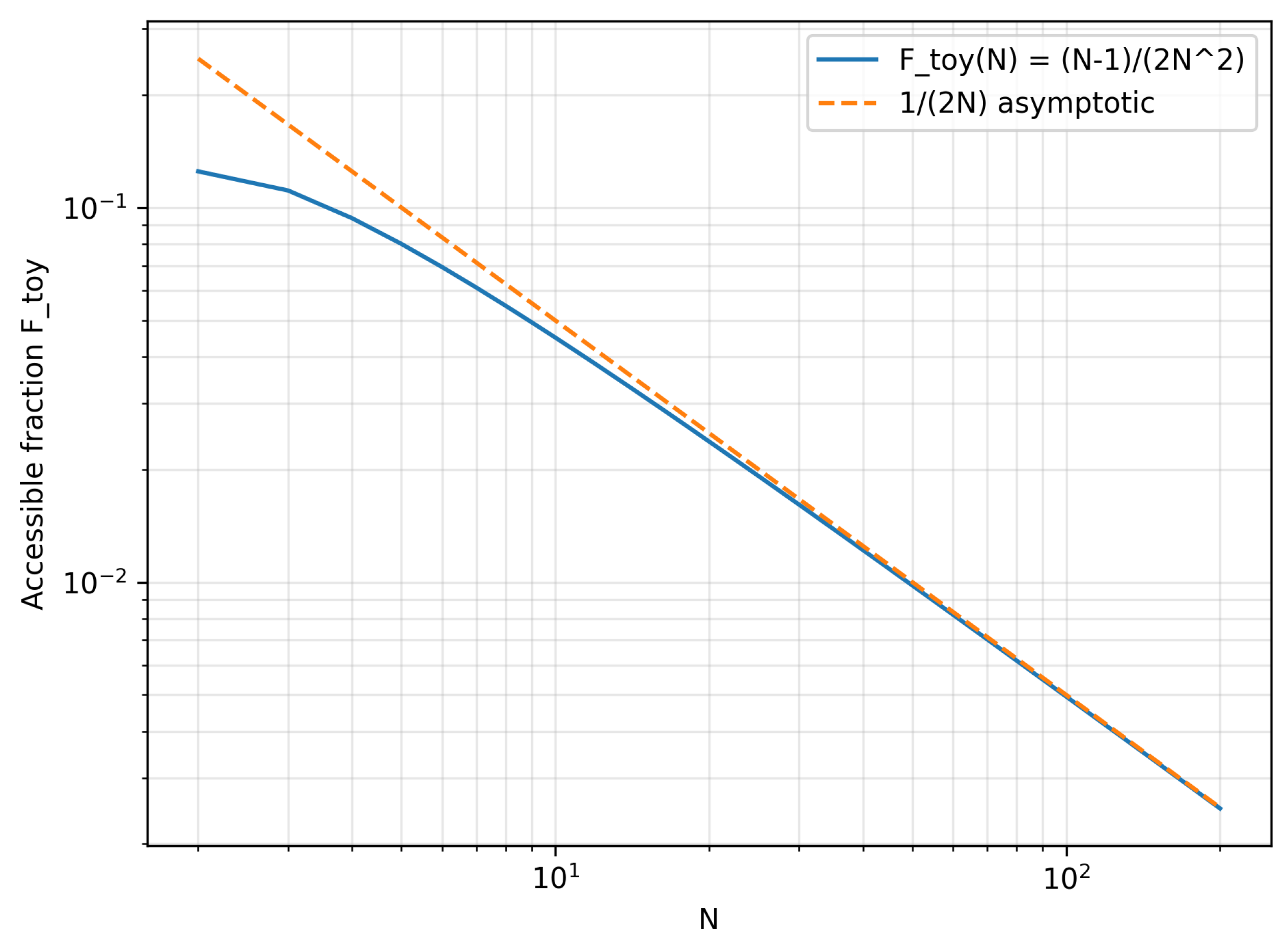
A simple numerical script confirms Eq. (A16) and illustrates the asymptotic boundary scaling. The log–log plot in Figure A2 shows that $F_{\mathrm{toy}}\left(N\right)$ rapidly approaches the $1/\left(2N\right)$ asymptote.

Reproducibility. The script that generates Figure A2 is available in the public GitHub repository https://github.com/davenagy86/HBMB.

Figure A2. Toy accessible fraction in the axial-gauge $U\left(1\right)$ zero-flux sector: $F_{\mathrm{toy}}\left(N\right)=(N-1)/\left(2N^2\right)$. The log–log plot demonstrates convergence to the boundary-type asymptotic scaling $1/\left(2N\right)$ for large N.

Figure A2. Toy accessible fraction in the axial-gauge $U\left(1\right)$ zero-flux sector: $F_{\mathrm{toy}}\left(N\right)=(N-1)/\left(2N^2\right)$. The log–log plot demonstrates convergence to the boundary-type asymptotic scaling $1/\left(2N\right)$ for large N.

Appendix C.1. QFT Side: Modular Energy in a Ball Region

Appendix C.1.1. Entanglement First Law

For small perturbations around the vacuum, the entanglement first law states (see e.g. [16])

$$\delta S_{\mathrm{EE}}=\delta \langle H_{\mathrm{mod}}\rangle ,$$

(A18)

where $S_{\mathrm{EE}}$ is the entanglement entropy of the region and $H_{\mathrm{mod}}$ is the modular Hamiltonian (e.g. via relative-entropy arguments).

Appendix C.1.2. Vacuum Modular Hamiltonian for a Ball

For a ball-shaped region $B\left(R\right)$ in flat spacetime, the vacuum modular Hamiltonian is local and can be written as

$$H_{\mathrm{mod}}=2\pi {\int }_{B\left(R\right)}{d}^{3}x{\displaystyle \frac{R^2-r^2}{2R}}{T}_{00}\left(x\right).$$

(A19)

The kernel $(R^2-r^2)/\left(2R\right)$ follows from the fact that the modular flow of a spherical region is generated by a conformal Killing vector that acts as a local boost near the entangling surface; see e.g. [15].

Geometric interpretation (modular flow → local Rindler structure). The same modular flow that yields the weight $(R^2-r^2)/\left(2R\right)$ also singles out a local boost symmetry at the boundary of the ball. This provides a natural bridge to the geometric side: near the entangling surface the modular Hamiltonian acts as the generator of a local Rindler time, suggesting a corresponding local null congruence and a horizon-like screen to which an area/entropy balance can be associated. In this sense, the ball-region modular energy is the QFT object most directly aligned with a local-horizon thermodynamic balance (cf. the local holographic screen (horizon) viewpoint of

citeJacobson1995).

Appendix C.1.3. Uniform Energy-Density Perturbation

Consider the simple perturbation

$$\delta \langle T_{00}\left(x\right)\rangle ={\rho }_0(r\le R),$$

(A20)

with ${\rho }_0$ small enough that the first-law regime applies.

Appendix C.1.4. Explicit Integration

Using Eqs. (A18)–(A20),

$$\begin{array}{cc}\hfill \delta \langle H_{\mathrm{mod}}\rangle & =2\pi {\int }_{B\left(R\right)}{d}^{3}x{\displaystyle \frac{R^2-r^2}{2R}}{\rho }_0\hfill \\ \hfill & =2\pi {\rho }_0{\int }_0^{R}4\pi r^{2}dr{\displaystyle \frac{R^2-r^2}{2R}}\hfill \\ \hfill & ={\displaystyle \frac{4{\pi }^2{\rho }_0}{R}}{\int }_0^R\left(R^2{r}^2-r^4\right)dr\hfill \\ \hfill & ={\displaystyle \frac{4{\pi }^2{\rho }_0}{R}}{\left[R^2{\displaystyle \frac{r^3}{3}}-{\displaystyle \frac{r^5}{5}}\right]}_0^R\hfill \\ \hfill & ={\displaystyle \frac{4{\pi }^2{\rho }_0}{R}}\left(R^2{\displaystyle \frac{R^3}{3}}-{\displaystyle \frac{R^5}{5}}\right)={\displaystyle \frac{4{\pi }^2{\rho }_0}{R}}\left({\displaystyle \frac{2}{15}}{R}^5\right)\hfill \\ \hfill & ={\displaystyle \frac{8{\pi }^2}{15}}{\rho }_0{R}^4.\hfill \end{array}$$

(A21)

Therefore,

$$\begin{array}{|c|}\hline \delta S_{\mathrm{EE}}=\delta \langle H_{\mathrm{mod}}\rangle ={\displaystyle \frac{8{\pi }^2}{15}}{\rho }_0{R}^4\\ \hline\end{array}\left({\displaystyle \frac{8{\pi }^2}{15}}\approx 5.263789\right).$$

(A22)

Appendix C.2. Geometric Side: Raychaudhuri fOcusing Toy Model

Appendix C.2.1. Raychaudhuri Equation and Area Transport

For a null geodesic congruence with tangent $k^a$ and affine parameter $\lambda$,

$${\displaystyle \frac{d\theta }{d\lambda }}=-{\displaystyle \frac{1}{2}}{\theta }^2-{\sigma }_{ab}{\sigma }^{ab}-R_{ab}{k}^a{k}^b\equiv -{\displaystyle \frac{1}{2}}{\theta }^2-{\sigma }_{ab}{\sigma }^{ab}-R_{kk},$$

(A23)

and the transported area evolves as

$${\displaystyle \frac{dA}{d\lambda }}=\theta \left(\lambda \right)A\left(\lambda \right).$$

(A24)

Appendix C.2.2. Controlled Assumptions and Interpretation

To isolate scaling rather than full dynamics, we adopt a regulated toy setup:

• negligible shear: ${\sigma }_{ab}{\sigma }^{ab}=0$,
• initially stationary screen: $\theta \left(0\right)=0$,
• approximately constant focusing: $R_{kk}\approx \mathrm{const}$ along the generators,
• linearised Einstein response for the perturbation: $R_{kk}=8\pi G{T}_{kk}\approx 8\pi G{\rho }_0$,
• affine range $\lambda \in [0,L]$ with $L=\eta R$ and $\eta =\mathcal{O}\left(1\right)$.

These assumptions are not meant to be realistic in detail; their role is to provide a transparent scaling test that can be compared to the modular-energy result above.

Appendix C.2.3. Weak-Focusing Limit and Explicit Area Change

In the weak-focusing regime $R_{kk}{L}^2\ll 1$, the quadratic term in $\theta$ is subleading, so

$$\theta \left(\lambda \right)\simeq -R_{kk}\lambda .$$

(A25)

Keeping only leading order in the perturbation, we may evaluate $A\left(\lambda \right)\simeq A_0$ inside the integral, giving

$$\begin{array}{cc}\hfill \delta A\equiv A\left(L\right)-A_0& \simeq {\int }_0^L\theta \left(\lambda \right)A_{0}d\lambda =-A_0{R}_{kk}{\int }_0^L\lambda d\lambda =-{\displaystyle \frac{A_0{R}_{kk}{L}^2}{2}}.\hfill \end{array}$$

(A26)

With $A_0=4\pi R^2$, $R_{kk}=8\pi G{\rho }_0$, and $L=\eta R$,

$$\begin{array}{|c|}\hline \delta A_{\mathrm{geom}}\simeq -16{\pi }^2{\eta }^{2}G{\rho }_0{R}^4\\ \hline\end{array}$$

(A27)

which reproduces the target scaling (A17).

Appendix C.3. Entropy-Balance Matching and the Role of ${\ell }_P^2$

Appendix C.3.1. HBMB Local Balance Condition

In the HBMB entropy-balance logic the screen contribution is written in Bekenstein–Hawking form,

$$\delta S_{\mathrm{BH}}={\displaystyle \frac{\delta A}{4{\ell }_P^2}},$$

(A28)

and the local balance is

$$\delta S_{\mathrm{BH}}+\delta S_{\mathrm{EE}}=0.$$

(A29)

Appendix C.3.2. Required Area Response

Using (A22) in (A29) gives the required area variation

$$\delta A_{\mathrm{req}}=-4{\ell }_P^2\delta S_{\mathrm{EE}}=-{\displaystyle \frac{32{\pi }^2}{15}}{\ell }_P^2{\rho }_0{R}^4.$$

(A30)

Appendix C.3.3. Matching and Normalization

The geometric toy model yields

$$\delta A_{\mathrm{geom}}=-C\left(\eta \right)G{\rho }_0{R}^4,C\left(\eta \right)=16{\pi }^2{\eta }^2.$$

(A31)

Equating $\delta A_{\mathrm{geom}}=\delta A_{\mathrm{req}}$ implies

$$C\left(\eta \right)G={\displaystyle \frac{32{\pi }^2}{15}}{\ell }_P^2.$$

(A32)

In natural units a fully normalised derivation fixes $C\left(\eta \right)$ so that ${\ell }_P^2=G$. Within the present toy parameterisation this corresponds to

$$C\left(\eta \right)={\displaystyle \frac{32{\pi }^2}{15}}⟺{\eta }^2={\displaystyle \frac{2}{15}}.$$

(A33)

This simply reflects that the affine range/normalisation is not fixed a priori in the toy setup, whereas the modular-flow weighting is fixed on the QFT side.

Appendix C.3.4. Restoring SI Units

Restoring ℏ and c makes explicit what is otherwise hidden by natural units:

$${\ell }_P^2={\displaystyle \frac{\hslash G}{c^3}}.$$

(A34)

With this substitution, the matching condition (A32) becomes an identity once the normalisation is fixed (e.g. by (A33)), and one recovers

$$\begin{array}{|c|}\hline G={\displaystyle \frac{{\ell }_P^2{c}^3}{\hslash }}\\ \hline\end{array}$$

(A35)

as expected. The key point for the main text is that ${\ell }_P^2$ appears here as the universal entropy density scale relating a screen area variation to an entropy variation; the modular-energy computation provides an operational, QFT-side normalisation target for that conversion when matched to focusing.

References

- J. D. Bekenstein, “Black Holes and Entropy,” Phys. Rev. D 7, 2333 (1973).
- S. W. Hawking, “Particle Creation by Black Holes,” Commun. Math. Phys. 43, 199 (1975).
- R. M. Wald, “Jacob Bekenstein and the Development of Black Hole Thermodynamics,” arXiv:1805.02302 [physics.hist-ph] (2018).
- T. Jacobson, “Thermodynamics of Spacetime: The Einstein Equation of State,” Phys. Rev. Lett. 75, 1260 (1995).
- G. ’t Hooft, “Dimensional Reduction in Quantum Gravity,” arXiv:gr-qc/9310026 (1993).
- L. Susskind, “The World as a Hologram,” J. Math. Phys. 36, 6377–6396 (1995), arXiv:hep-th/9409089. [CrossRef]
- R. Bousso, “The Holographic Principle,” Rev. Mod. Phys. 74, 825–874 (2002), arXiv:hep-th/0203101. [CrossRef]
- J.-P. Uzan, “Varying Constants, Gravitation and Cosmology,” Living Rev. Relativ. 14, 2 (2011), arXiv:1009.5514. [CrossRef]
- C. J. A. P. Martins, “The status of varying constants: a review of the physics, searches and implications,” Rep. Prog. Phys. 80, 126902 (2017), arXiv:1709.02923. [CrossRef]
- W. Donnelly and A. C. Wall, “Entanglement Entropy of Electromagnetic Edge Modes,” Phys. Rev. Lett. 114, 111603 (2015), arXiv:1412.1895 [hep-th].
- W. Donnelly and A. C. Wall, “Geometric Entropy and Edge Modes of the Electromagnetic Field,” arXiv:1506.05792 [hep-th] (2015).
- K. S. Thorne, R. H. Price, and D. A. Macdonald (eds.), Black Holes: The Membrane Paradigm, Yale University Press (1986).
- S. W. Hawking, M. J. Perry, and A. Strominger, “Soft Hair on Black Holes,” Phys. Rev. Lett. 116, 231301 (2016), arXiv:1601.00921 [hep-th].
- H. Casini, M. Huerta and J. A. Rosabal, “Remarks on entanglement entropy for gauge fields,” Phys. Rev. D 89, no.8, 085012 (2014), arXiv:1312.1183 [hep-th].
- H. Casini, M. Huerta and R. C. Myers, “Towards a derivation of holographic entanglement entropy,” JHEP 05, 036 (2011), arXiv:1102.0440 [hep-th].
- N. Lashkari, M. B. McDermott and M. Van Raamsdonk, “Gravitational dynamics from entanglement thermodynamics,” JHEP 04, 195 (2014), arXiv:1308.3716 [hep-th].
- E. Tiesinga, P. J. Mohr, D. B. Newell, and B. N. Taylor, “CODATA recommended values of the fundamental physical constants: 2018,” Rev. Mod. Phys. 93, 025010 (2021). [CrossRef]
- D. Nagy, “A First-Principles Derivation of the Fine-Structure Constant from Holographic Bit–Mode Balance,” preprint (2025). https://osf.io/preprints/osf/hw2je.
- D. Nagy, “Holographic Vacuum Energy from Quantized Horizons,” preprint (2025). https://osf.io/preprints/osf/m8t6h.
- D. Nagy, “Basics of a Geometry-Independent HBMB Holographic Principle: From Horizon Bits to Bulk Wavefunctions – Part I,” Preprints (2026). [CrossRef]
- A. Hamilton, D. Kabat, G. Lifschytz, D. A. Lowe, “Holographic Representation of Local Bulk Operators,” Phys. Rev. D 74, 066009 (2006), arXiv:hep-th/0606141.
- A. J. Murphy, “Closed-Form Derivation of the Fine-Structure Constant from U(1) Configuration Space Geometry,” preprint (2025). [CrossRef]
- M. K. Parikh and F. Wilczek, “An action for black hole membranes,” Phys. Rev. D 58, 064011 (1998).
- K. von Klitzing, G. Dorda, and M. Pepper, “New method for high-accuracy determination of the fine-structure constant based on quantized Hall resistance,” Phys. Rev. Lett. 45, 494–497 (1980).
- T. Damour, “Black-hole eddy currents,” Phys. Rev. D 18, 3598 (1978).
- R. L. Znajek, “The electric and magnetic conductivity of a Kerr hole,” Mon. Not. R. Astron. Soc. 185, 833–840 (1978).
- B. Jeckelmann and B. Jeanneret, “The quantum Hall effect as an electrical resistance standard,” Rep. Prog. Phys. 64, 1603–1655 (2001).
- P. J. Mohr, D. B. Newell, and B. N. Taylor, “CODATA recommended values of the fundamental physical constants: 2014,” Rev. Mod. Phys. 88, 035009 (2016).
- J. D. Jackson, Classical Electrodynamics, 3rd ed., John Wiley & Sons, New York (1999).
- A. Chodos, R. L. Jaffe, K. Johnson, C. B. Thorn, and V. F. Weisskopf, “New extended model of hadrons,” Phys. Rev. D 9, 3471 (1974).
- R. Camporesi and A. Higuchi, “On the eigenfunctions of the Dirac operator on spheres and real hyperbolic spaces,” J. Geom. Phys. 20, 1–18 (1996).
- D. V. Vassilevich, “Heat kernel expansion: user’s manual,” Phys. Rept. 388, 279–360 (2003).
- P. B. Gilkey, Invariance Theory, the Heat Equation, and the Atiyah–Singer Index Theorem, 2nd ed., CRC Press (1995).
- K. Kirsten and A. J. McKane, “Functional determinants by contour integration methods”, Ann. Phys. 308, 502 (2003).
- G. V. Dunne and K. Kirsten, “Functional determinants for radial operators,” J. Phys. A 39, 11915–11928 (2006), arXiv:hep-th/0607066. [CrossRef]
- M. E. Peskin and D. V. Schroeder, An Introduction to Quantum Field Theory, Addison–Wesley, Reading, MA (1995).
- J. B. Kogut, “An Introduction to Lattice Gauge Theory and Spin Systems,” Rev. Mod. Phys. 51, 659 (1979).
- R. Kubo, “Statistical-Mechanical Theory of Irreversible Processes. I. General Theory and Simple Applications to Magnetic and Conduction Problems,” J. Phys. Soc. Jpn. 12, 570–586 (1957).
- R. Kubo, “The fluctuation-dissipation theorem,” Rep. Prog. Phys. 29, 255–284 (1966).
- G. D. Mahan, Many-Particle Physics, 3rd ed., Kluwer Academic / Plenum Publishers, New York (2000).
- P. Di Francesco, P. Mathieu, and D. Sénéchal, Conformal Field Theory, Springer, New York (1997).
- P. Ginsparg, “Applied Conformal Field Theory,” in Fields, Strings and Critical Phenomena (Les Houches 1988), eds. E. Brézin and J. Zinn-Justin, North-Holland (1989), arXiv:hep-th/9108028.
- X.-G. Wen, Quantum Field Theory of Many-Body Systems, Oxford University Press, Oxford (2004).