
Submitted:
23 November 2025
Posted:
24 November 2025
You are already at the latest version
Abstract
Bike-sharing services contribute to reducing emissions and conserving natural resources within urban transportation systems. They also promote public health by encouraging physical activity and generate economic benefits through shorter travel times, lower transportation costs, and decreased demand for parking infrastructure. This paper examines the use of shared micro-mobility services in the Italian cities of Firenze and Bologna, based on an analysis of GPS origin–destination data and associated temporal coordinates provided by the RideMovi company. Given the still limited number of studies on free-floating and electric bike-sharing systems, the objective of this work is to quantify the performance of electric bikes and E-scooters in bike-sharing schemes and compare it to traditional, muscular bikes. Results show that E-bikes are from 22 to 26\% faster on average with respect to muscular bikes, extending trip range in Bologna, but not in Firenze. Electric modes attract more users than traditional bikes, E-bikes have from 40 to 128\% higher daily turnover in Bologna and Firenze, and E-scooters from 33 to 62\% higher in Firenze with respect to traditional bikes. Overall, turnover is fairly low, with less than 2 trips per vehicle per day. The performance is measured in terms of trip duration, speed, and distance. Further characteristics such as daily turnover by transport mode, trip purpose, and user type are investigated and compared. The results aim to support planners and operators in designing and managing more efficient and user-oriented services.
Keywords:
bike-sharing
; free float systems
; e-bikes
; e-scooters
; electric mobility
; shared micromobility
; ridership
; decarbonization
1. Introduction
Bike-sharing programs (BSPs) have become an integral component of contemporary urban transportation, reflecting the growing need to move away from motorized vehicles to more sustainable travel modes [1]. Their rapid expansion helps address pressing urban challenges, most notably traffic congestion and poor air quality, since motorized transport remains a major source of greenhouse gas emissions worldwide [2]. By integrating and promoting bicycles into urban mobility networks, BSPs contribute to emission reductions and the conservation of natural resources. In Shanghai, for example, bike-sharing was estimated to save 8,358 tons of fuel annually, resulting in reductions in carbon dioxide and nitrogen oxide emissions and measurable improvements in air quality [3]. Beyond environmental benefits, BSPs promote public health by encouraging physical activity and deliver economic benefits through shorter travel times, lower transportation costs, and reduced demand for parking infrastructure. Together, these outcomes position BSPs as an effective strategy for cleaner air, decarbonization, more efficient mobility, and improved population health [4,5], while supporting a larger shift towards cycling as an efficient mode of transport [6]. Currently, bike-sharing programs operate primarily in two formats: station-based and dockless. Station-based systems (DBS) rely on fixed docking stations, where users collect and return bicycles, while dockless systems (DLBS or Free-float, FFS) offer greater flexibility by allowing bicycles to be parked and locked anywhere within the designated service area. This flexibility, however, has a counterpart in uncontrolled—and at times obstructive—parking of shared vehicles. DLBS operations leverage GPS and mobile technology for bicycle tracking and rental via smartphone applications. The resulting free-floating model has driven the rapid global diffusion of DLBS, positioning it as a promising approach to improving urban mobility and advancing environmental sustainability. Nevertheless, DLBS also faces persistent challenges, including bicycle theft, vandalism, the distribution of bicycles in the territory, obstructive parking, and difficulties in ensuring reliable tracking of the bike position [7]. On the other hand, conventional (or “muscular”) bicycles have traditionally formed the backbone of bike-sharing systems, primarily serving shorter trips with demand strongly influenced by terrain morphology [7]. By contrast, electric bicycles (e-bikes) provide motorized assistance, markedly enhancing their practicality and appeal: e-bikes are particularly effective for navigating hilly areas [8] and for enabling longer travel distances [9] and for reducing travel time. Their introduction has broadened the shared cycling market by attracting new user groups and lowering barriers for individuals with physical limitations [10]. While initially complementing conventional bicycle use, e-bikes often become a substitute over time—reducing demand for muscular bicycles yet substantially increasing overall shared cycling activity [9]. Moreover, e-bikes, considering their enhanced performances, show greater potential for replacing car trips than their muscular counterparts [11]. A wide range of factors shapes usage patterns in bike-sharing programs (BSPs), as widely studied in the recent review from Mafi et al. [12]. Among the most important factors, there are weather conditions, including temperature [13,14], precipitation [15], wind speed [16], humidity, and seasonal variation [14], which can significantly affect ridership levels. Built environment and land-use characteristics also matter, such as the availability of cycling infrastructure [17], perceived safety [18], topography [19], land-use mix, and the degree of integration with public transport or mobility hubs [20,21,22]. In addition, demographic attributes, including age, gender, income, education level, and motor vehicle ownership, are important determinants of BSP usage [23,24,25,26]. Finally, vehicle provision and service fees have a strong impact on usage of these transport services.
In Italy, the bike-sharing landscape has been shifting toward free-floating systems. According to the 2024 report of the Italian National Shared Mobility Observatory [27], in 2016 all available services were station-based; beginning in 2017, the first dockless solutions were introduced. By 2023, of 47 bike-sharing services, 30 were dockless, with 77% of the national fleet operating in free-float mode. The same report ranks Bologna and Florence third and fourth, respectively, for electric fleet size. Overall, the market is moving toward electrification, with e-bikes accounting for 67% of the Italian shared bicycle fleet.
Given the limited number of studies on free-floating and electric bike-sharing and scooter-sharing services [8], this paper aims to identify how BSS is used, based on revealed-preference data from users’ trips in two medium-size Italian cities. The findings are intended to assist planners and operators in designing better services, also by better understanding the differences between electric and muscular modes of shared micro-mobility. In the literature, GPS data have proven highly valuable for studying shared micromobility across multiple dimensions, including spatial analyses of territorial and behavioral factors that promote bike and scooter use [28,29,30], intra-week and gender differences in usage [31], contrasts between privately owned and shared bicycles [32], equitable access to transport [33], the impacts of the COVID-19 pandemic [34], and the environmental benefits of bike sharing [35]. GPS records embed users’ revealed preferences with spatial context, offering considerable flexibility for diverse study designs, and new methods are emerging to acquire such datasets with high reliability and low effort [36]. Although many studies leverage GPS information, the authors are aware of only one case that attempts path reconstruction when full traces are unavailable [34], and even there the approach is used primarily to improve distance estimation compared with the Euclidean alternative.
This study assesses shared services using descriptive statistics and temporal and spatial analyses. We examine daily demand patterns, weekly dynamics of trip length, duration, and speed, daily turnover and productivity across trip-distance ranges, and monthly variations in trip volume, fleet size, and turnover, with comparisons across available modes. A productivity analysis quantifies trips per vehicle by mode for different trip-distance ranges, providing operators and planners with insight into the distances typically served by each mode. Temporal analysis at the week level highlights differences between working days and weekends, while monthly analysis reveals seasonality. The spatial analysis divides each city into 250 × 250 meter grid cells to identify zones with a surplus or deficit of vehicles, that is, where more trips end than begin, and vice versa. A key contribution of this study is the ability to derive insights that typically require full GPS traces, using only origin–destination and time records. By applying routing methods to microscopically detailed network models, we reconstruct plausible paths and analyze trip length, average speed, and temporal patterns. This approach broadens the usefulness of operator data, reduces reliance on continuous tracking, and provides planners and operators with actionable information even when only minimal trip attributes are available. The method is also advantageous from a privacy perspective, since bike-sharing data can be sensitive due to real-time tracking of individuals and operators seldom share complete traces.
This paper is organized into six sections. Methodology outlines preprocessing steps and explains the procedures used to reconstruct trips from GPS origin and destination points with their timestamps. This procedure enables the reconstruction of likely paths and the estimation of trip length and average speed, and it supports data filtering to remove anomalous trips. Case Study describes the main characteristics of the two Italian cities. Dataset Description and Preparation details the dataset and the application of the methodology to Florence and Bologna. Results presents descriptive statistics, monthly dynamics, mode-specific patterns, and spatial analysis together with plausible interpretations for both cities. Discussion synthesizes the findings across the two case studies, assesses their implications for planning and operations, and compares the cases. Conclusions summarize the main contributions, highlight practical points for operators and planners, and indicate priorities for future research.
2. Methodology
While the use of GPS origin–destination data in micromobility analyses is not new, such data are often employed without reconstructing the underlying trip. Many studies rely on Euclidean distances, and, to the authors’ knowledge, the only example of trip reconstruction in this area applies a standard shortest-path assignment on a subset of the transport network to improve distance estimation over the Euclidean measure [34]. In contrast, our study uses a detailed microscopic network and a refined shortest-path method previously calibrated for bicycle-trip reconstruction, and validates the resulting trips against full GPS traces from a prior study. The process used to reconstruct trips from OD GPS data is illustrated in Figure 1.
For privacy and commercial reasons, operators often do not provide full GPS traces. More commonly, datasets include only latitude, longitude, start and end times, vehicle type, and vehicle ID. In this study, the absence of full traces required routing to reconstruct likely paths and to estimate trip length and average speed. To enable reconstruction, the dataset must be map-matched to the urban network, often imported from OpenStreetMap (OSM). The imported network should be cleaned and refined by clustering nodes into coherent intersections and ensuring the correct representation of existing bicycle lanes. GPS origin and destination records can be map-matched within HybridPY [37,38], an open-source microsimulation suite developed at the University of Bologna for the SUMO engine. After map-matching origin and destination points, trips are routed to reconstruct a plausible path. The method applies a shortest-trip criterion that assigns a slightly more favorable cost to reserved bicycle lanes; full details are provided in [39]. Once trips are reconstructed, anomalous records must be filtered, since round trips or trajectories with substantial detours are difficult to infer from origin–destination data alone. Filtering is applied to trip distance, trip time, and space-average speed. Trip distance is derived from routing, trip time is taken directly from the timestamps of the dataset, and space-average speed is computed as distance over time. Finally, validation can be performed by comparing reconstructed trips with a sample of continuous GPS traces, which allow reconstruction of actual routes and speed profiles. When only origin and destination times are available, validation can also rely on comparing the distribution of average trip speeds with those computed from continuous traces for the same case study. A validation procedure specific to our dataset is presented in the Case study section.
3. Case Study
The methods shown in the Methodology section has been applied to the two case studies of Florence and Bologna, two medium-sized cities in central northern Italy with comparable territory and population. Florence covers 102 km² and has approximately 362 thousand inhabitants; Bologna covers 140 km² and has approximately 393 thousand inhabitants. The historic center of Florence, a UNESCO World Heritage Site, spans about 5 km², while Bologna’s historic center extends over roughly 4.5 km². Florence experiences heavy year-round tourism, about 12.750 million visitors in 2023 [40]. Bologna has a lower tourist load than Florence, but a large share of university students live in the city. In territorial terms the two cities are similar; however, differences in user composition: tourists in Florence and university students in Bologna, can substantially influence demand for bike-sharing services. Both cities have a Sustainable Urban Mobility Plan (PUMS, Piano Urbano della Mobilità Sostenibile). Bologna was the first Italian city to adopt a metropolitan SUMP, formally approved in 2019, while Florence followed with its metropolitan plan in 2021. Both plans align with EU climate targets, modal shift, and integrated mobility systems. Bologna’s strategy centers on the 1,000 km “Bicipolitana” cycling network, which has helped attract new riders [41], a new tramway system, and a regionally coordinated approach to micromobility and car sharing. Florence’s plan builds on its existing tram infrastructure, expands the cycling network toward a 200 km target, and introduces intermodal incentives such as free shared-bike access for public transport users. Both cities articulate a Mobility-as-a-Service vision, though no operational platform is yet deployed. Bologna’s PUMS sets an objective to integrate services, especially around intermodality and smart mobility, but does not specify a functioning MaaS platform. It calls for digitalization and service aggregation, linking bike sharing, car sharing, and public transport within a common platform. Florence’s plan likewise emphasizes intermodal integration and frames MaaS as a future development path, highlighting digital tools and “smart mobility” without concrete deliverables. Although public funding has been allocated to similar initiatives in several Italian cities, MaaS remains largely at the pilot stage in practice [42].
Regarding service type, both Florence and Bologna operate free-floating systems, primarily served by electric bicycles. RideMovi, the main provider in both cities, offers three sharing options in Florence: bikes, e-bikes, and e-scooters, while in Bologna it offers two: bikes and e-bikes.
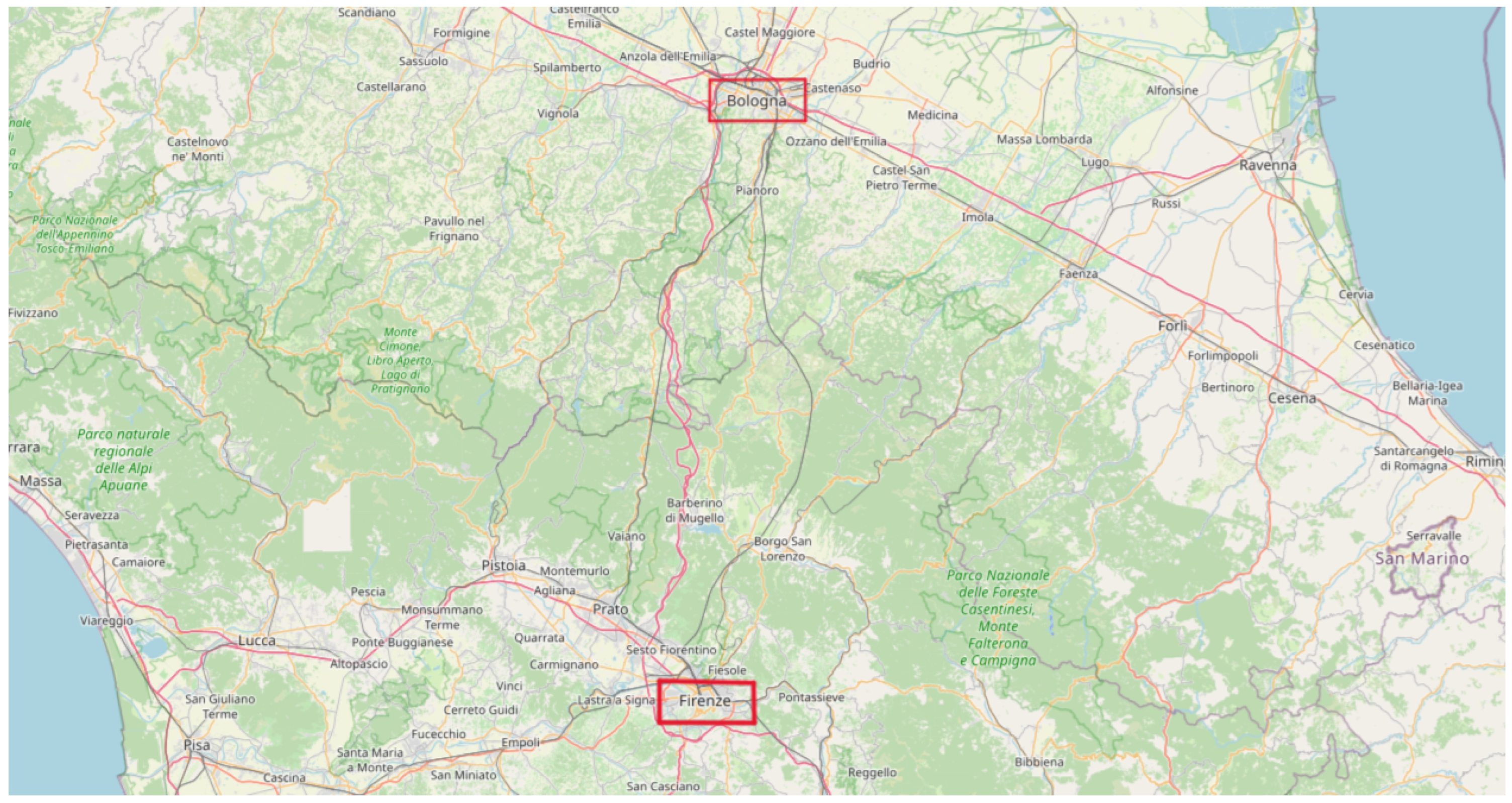
Figure 2.
Map of Italy with the two case studies highlighted in red. Map downloaded from OpenStreetMap, OpenStreetMap Foundation, under CC BY-SA 3.0 license.
Figure 2.
Map of Italy with the two case studies highlighted in red. Map downloaded from OpenStreetMap, OpenStreetMap Foundation, under CC BY-SA 3.0 license.
4. Dataset Description and Preparation
RideMovi and Società Reti e Mobilità provided GPS data for Florence and Bologna’s shared micromobility services for 2023 as comma-separated value files. The dataset includes the latitude, longitude, and time of trip origins and destinations, the vehicle type, and the vehicle ID; individual trips do not contain full GPS trajectories. The data were map-matched to the Bologna and Florence urban networks in HybridPY [37,38].
The Bologna network was imported from OpenStreetMap (OSM) and has been refined and regularly updated through multiple projects. Florence’s network was imported from OSM and subsequently cleaned and updated to support reliable map-matching and routing for bicycles, e-bikes, and e-scooters within the HybridPY environment by clustering intersection and ensuring bikeway lanes continuity. After map-matching the origin and destination of each trip to the SUMO network model, we performed the routing with the method of Schweizer et al. [39], as outlined in Section 2. The extracted data were filtered to remove trips with anomalies. Filtering was applied to trip distance (from routing estimation), trip time (from the data), and space-average speed (computed as distance over time, thus an estimate). Trips that were too short in distance or time, or unrealistically slow or fast, were removed. Such filtered trips may reflect errors in the dataset or incorrect routing. Routing errors can occur for round-trips or for trips with multiple detours between origin and destination. The authors acknowledge that these trips are of interest, but with the current data availability from the operator, that is, origin–destination points only, there is no reliable way to distinguish non-direct trips from data errors. The filtering thresholds and results are reported in Table 1. Trips with reconstructed lengths below 400 meters are excluded, since they can be covered in just over 100 seconds of motion. As unlocking and locking times are included, these would excessively distort the estimated average speed. Very short trips should also be removed, as they could be round trips with close origin and destination; in these cases the route reconstruction would fail. Rentals shorter than 3 minutes or longer than about 40 minutes are excluded as not representative: the former are too brief, and the latter may include substantial pauses that cannot be reconstructed from origin–destination data. Trips with average speeds below 1 m/s are discarded as slower than walking pace, while those above 6.94 m/s (25 km/h) are removed as unrealistically fast even for an e-bike with a 25 km/h speed limit for pedal assistance. The filtering ranges and retained trip shares are reported in Table 1.
Validation of the reconstructed trips was carried out by comparing them with a previous study on bicycle mobility in Bologna. Rupi et al. [43] analyzed continuous GPS traces from the European Cycling Challenge 2016, which allowed the authors to reconstruct actual routes and speed profiles. Since our dataset contains only origin and destination points, we validated the routing by comparing the distribution of average trip speeds from our sample with those reported by Rupi et al. (2020). Rupi et al. (2020) derived their average speed distribution from speed profiles of trips undertaken during working days between 05:00 and 11:00 in May 2016 in Bologna during the European Cycling Challenge (https://cyclingchallenge.eu/ecc2016). To obtain a comparable sample, we compare our reconstructed trips from May 2023 that started between 05:00 and 11:00 on working days, restricting the analysis to muscular bicycles, as only muscular bikes were used in May 2016. Several differences should be noted: (i) Rupi et al. measured speeds for participants who volunteered for data collection, which may bias the sample toward experienced or cycling-enthusiast users; (ii) they assumed a fixed time for unlocking, on the basis that users had already started app tracking, and subtracted this from total trip time; (iii) our trip times include unlocking and locking for shared bikes, even though these durations are generally quite short in the RideMovi service; (iv) our filtering is inherently less precise because we lack full GPS traces to select the most representative trips; and (v) limiting the time window and bike type to muscular bicycles yields a smaller sample, since muscular shared bikes were much less than e-bikes in Bologna in 2023.
Average speed distributions are broadly similar. An 18% discrepancy was expected, as Rupi et al. [44], using the same GPS traces of Rupi et al. (2020), found that cyclists tend to travel routes about 20% longer than the shortest path to avoid high-traffic roads. Consequently, our reconstruction likely underestimates the true route length and yields speeds that are approximately 20% lower (see Table 2).
We also compared speed distributions with similar European case studies [45,46,47,48]. Methods in those studies include GPS-trace analysis, video recording, and built-on speed sensors. In our data, average speeds range from 2.90 to 3.45 m/s for muscular bicycles and from 3.53 to 4.35 m/s for e-bikes. In the reviewed cases, reported averages range from 2.50 to 4.25 m/s for bicycles and from 4.83 to 6.00 m/s for e-bikes and mixed samples. Our averages lie at the lower end of these ranges, consistent with the estimated 18% underestimation of average speed in our dataset. Other factors may impact average speeds such as climate or street-layout.

Table 3.
Comparison of average values of trip speed with other EU case studies. Please note that here the speed is calculated on trips filtered based on the values in Table 1
Table 3.
Comparison of average values of trip speed with other EU case studies. Please note that here the speed is calculated on trips filtered based on the values in Table 1
| Study | Location | Vehicle Type | Data acquisition Method | Av. Speed [m/s] | Standard Deviation [m/s] |
|---|---|---|---|---|---|
| This Study | Bologna (Italy) | Bike | GPS o/d | 2.90 | 0.88 |
| This Study | Bologna (Italy) | E-Bike | GPS o/d | 3.53 | 1.10 |
| This Study | Florence (Italy) | Bike | GPS o/d | 3.45 | 1.08 |
| This Study | Florence (Italy) | E-Bike | GPS o/d | 4.35 | 1.27 |
| Ul-Abdin et al. [45] | Belgium | Bike and E-Bike | GPS Trace | 4.36 | 1.69 |
| Lyubenov et al. [46] | Bulgaria | Bike | GPS Trace | 2.50 | 0.05 |
| Paulsen et al. [47] | Denmark | Bike and E-Bike | Video Recording | 6.00 | 1.00 |
| Schleinitz et al. [48] | Germany | Bike | Speed sensor | 4.25 | 0.64 |
| Schleinitz et al. [48] | Germany | E-Bike | Speed sensor | 4.83 | 1.22 |
5. Results
This section shows the results obtained for Florence and Bologna.
5.1. Florence
After presenting the most important aggregate results considering muscular bikes, electric bikes, and scooters, the following sub-sections focus on spatial analysis, monthly variations, productivity, and usage.
5.1.1. Overview
As shown in Figure 3, most of the fleet consists of e-bikes, with 3,236 unique vehicles active in 2023, although Florence still maintains a large number of conventional bicycles and a substantial e-scooter fleet, with 1,885 and 1,005 vehicles respectively.
Figure 4 presents the distributions of trip length, average trip speed, and trip duration for the retained data of Florence used in the analysis. As described in the Methods section, only trip duration comes directly from the dataset, whereas trip length was estimated via routing, and average speed is a space-average value computed as routed trip length over trip duration. Trip duration is distinctly left-skewed across all modes, and trip length shows a similar pattern. By contrast, average speed follows a distribution close to normal, at least for bikes and e-bikes. All modes span comparable distance ranges, even if the average distance for e-scooter is about 15% lower than the average values of the other modes: although e-bikes reach longer distances, each mode appears capable of serving similar travel-distance needs. Nevertheless, the speed of electric modes remain clearly superior, especially for e-bikes, as reported in Table 4 e-bikes are on average 26% faster than muscular bike and 15% faster than e-scooters. Moreover, trips on e-bikes are on average 20% shorter in duration with respect to muscular bikes, thus providing a significant time saving for the user.
5.1.2. Spatial Analysis
Spatial analysis was conducted by counting trip origins and destinations within 250 × 250 meter grid cells. Figure 5a,b show that trips are concentrated in the historic center, the city’s main tourist area, with particularly high density around Santa Maria Novella station. Outside the center, two additional hotspots emerge: one in the northwest, near a bus station and a university complex, and another to the south at the edge of the Boboli Gardens. Panel Figure 5c reports the net annual flow for each cell. Blue cells indicate zones where more trips begin than end, signaling a deficit of vehicles, and vice versa. The most pronounced asymmetry occurs at the train station, which exhibits a large vehicle deficit, whereas most of the remaining central area is relatively balanced. The southern edge of the Boboli Gardens also shows a deficit, likely reflecting users who enter from the city-center side and use shared vehicles to exit on the opposite side of the park.
5.1.3. Monthly Variations
The dataset was analyzed to assess intra-year variation by month. Figure 6 reports monthly values for total trips, average daily turnover, and fleet composition throughout 2023. The number of trips varied substantially over the year, although trends differed by mode. All modes exhibited lower usage in January, February, March, November, and December. In addition, only e-bikes and bicycles showed a further decline in August, whereas e-scooters maintained high usage during this summer month.
Monthly average daily turnover was computed as the total number of trips for a given vehicle type in a month divided by the number of unique vehicle IDs observed in that month and by the number of active days in the same month, where active days were defined as days with at least one recorded trip. This measure is sensitive to abrupt changes in fleet composition within the same month. Given its temporal resolution relative to the yearly measure, it is more suitable for comparing turnover across modes. E-bikes recorded the highest turnover in every month except August, ranging from a low in January of 1.030 trips per vehicle per day to a peak in October of 2.052 trips/vehicle/day. The lower August turnover may reflect the turnover definition, since August also saw an increase in the e-bike fleet size. In addition, August in Florence is very hot and coincides with a vacation period for many Italian workers, so that multiple factors may be at play. Turnover for e-scooters follows a pattern similar to that of e-bikes. The sharp decline in May can be attributed to the substantial increase in e-scooter fleet size during that month. August shows a smaller decrease than for e-bikes, while the larger reduction occurs in September. Traditional bicycles exhibit the same pattern observed for e-bikes. Overall, e-bikes dominate trip production intensity, with e-scooters close behind, whereas bicycles perform comparatively poorly, often generating fewer than one trip per vehicle per day. Fleet composition remained generally stable over the period, with the exception of e-scooters, which experienced a sudden increase in May from 290 to 569 vehicles. Despite their lower productivity, traditional bikes still remain a large share of Florence’s shared fleet, with approximately 1,400 vehicles.
5.1.4. Productivity Analysis
Examining turnover across trip-length ranges, as shown in Figure 7, helps identify the optimal operating range for each mode. Trip length may correlate with city size, land-use mix, and population habits, so understanding the distance ranges in which a service is most valued can guide planners in calibrating the fleet mix to meet expected needs. This is relevant for operators, since it indicates which vehicles are most productive in terms of trips per vehicle, and for planners, who can optimize fleet size and composition to align supply with demand. This approach is not a substitute for stated- or revealed-preference surveys in all contexts; However, the GPS data may be considered a kind of revealed preference survey without person attributes, as the trips were actually undertaken with different modes. So, it can still support the development of useful heuristics. The various examined modes should be compared with caution, since the figures reported are yearly averages that reflect the total fleet size. Because fleet size varies over the year, whereas it is generally more stable within a single month, the yearly turnover can be deflated when fleet sizes change substantially. This occurs in our case: the e-scooter fleet expanded rapidly in May, which lowers the yearly e-scooter turnover slightly below that of bicycles. As shown in Figure 6, the monthly turnover, less exposed to errors from fleet changes, is Pareto-superior for e-scooters relative to muscular bicycles. This limitation is not severe because each mode’s distribution remains proportional and comparable with itself across trip-distance ranges. It is therefore still possible to identify where a given mode is more or less productive, and to compare modes with appropriate caution. In general, the shared mobility services studied are most productive in the 800–2800 meter range. Bicycles and e-scooters are used more frequently for trips between 800 and 2400 meters, whereas e-bikes maintain strong trip production even at 3600 meters. Overall, e-bikes are Pareto-superior in turnover relative to the other modes. Except for very short trips, up to 800 meters, the e-bike exhibits a much higher turnover.
5.1.5. Use and Demand Patterns
Another interesting aspect is how the services are used across days of the week. Figure 8 presents box plots for all three modes and three trip parameters, trip length, average trip speed, and trip duration from Monday to Sunday. Trip length and average speed remain broadly constant in distribution throughout the week, with no notable differences between weekdays and weekends, as also highlighted in Table 5. Only trip duration shifts toward higher values on weekends, although interpretation is limited because the change is on the order of 60 seconds, which is the minimum time aggregation in the Florence dataset. Since the means also show no substantial differences, it appears that most users display similar behavior on weekdays and weekends.
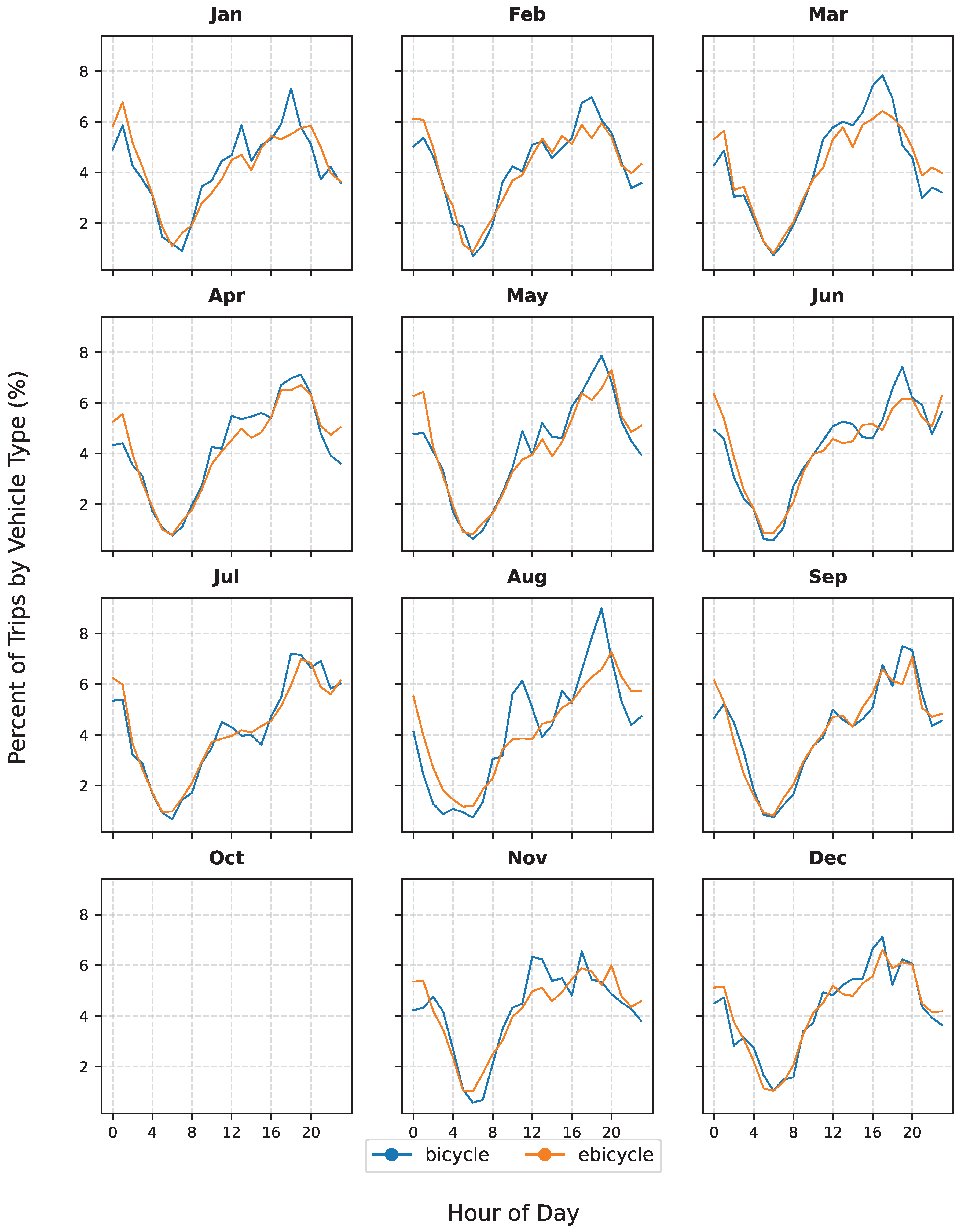
Finally, we examine the average daily demand pattern for weekdays and weekends. Figure 9 and Figure 10 show the hourly percentage of trip starts for weekdays and weekends, respectively. On weekdays, demand patterns are similar for bikes and e-bikes, but different for e-scooters. Bicycles and e-bicycles show two major peaks and one minor peak: a morning peak at 08:00, an afternoon peak at 18:00, and a smaller peak at 23:00 following a rapid contraction during dinner hours, 20:00 to 22:00. E-scooters begin with modest morning demand, rise to a peak at 18:00, peak again at 23:00, and retain slightly higher usage during the late night. All three modes reach a minimum at 05:00. Weekend patterns shift markedly. Bicycles and e-bikes show higher demand beginning around 09:00 and peak at 17:00, with a more uniform distribution across the day than on weekdays. Both modes contract during dinner hours, 20:00 to 22:00, then rise again to a peak at 00:00, indicating a stronger concentration of nighttime use. E-scooters follow a similar weekend profile, with lower morning demand and higher nighttime demand compared with the two bicycle modes. The same plots were examined month by month to identify intra-year variation. However, Figure A1 and Figure A2 indicate that, for weekdays and weekends respectively, there are no major pattern changes across months, only fluctuations around the patterns already described.
5.2. Bologna
This subsection contains the results for Bologna, considering only e-bikes and muscular bikes. After the most important aggregate results are presented, the following sub-sections focus on spatial analysis, monthly variations, productivity, and usage.
5.2.1. Overview
As shown in Figure 11, most of the fleet consists of e-bikes, with 3,239 unique vehicles active in 2023 and only 526 traditional bicycles. Indeed, Bologna’s service has transitioned to an almost fully electric fleet.
Figure 12 presents the distributions of trip length, average trip speed, and trip duration for the retained data. Trip duration is distinctly left-skewed across modes, and trip length shows a similar pattern. By contrast, average speed follows a distribution close to normal. Unlike Florence, the trip distance is much greater for e-bikes compared to muscular bikes (+19%), and trip durations are almost the same for both muscular and electric bikes. Table 6 reports the means and some percentiles of these distributions.
5.2.2. Spatial Analysis
Spatial analysis was performed by counting trip origins and destinations within 250 × 250 meter grid cells. Figure 13a,b show that activity is most intense in the city center, near Piazza Maggiore and the Asinelli and Garisenda towers, where commercial activity and tourist attractions are concentrated. Another hotspot appears to the north around the central railway station. Panel Figure 13c reports the net annual flow for each cell. Blue cells indicate zones where more trips begin than end, signaling a bicycle deficit, and red cells indicate the opposite. In Bologna, blue cells cluster in the city center, while red cells are dispersed across the grid, indicating a general outward asymmetry of demand from the center.
5.2.3. Monthly Variations
The dataset was analyzed to assess intra-year variation by month. Figure 14 reports monthly values for total trips, average daily turnover, and fleet composition for 2023, with October omitted due to missing data. Trip volumes varied substantially over the year, with both electric and standard bicycles recording fewer trips in January and peaking in June and September, similar to Florence. Monthly average daily turnover was computed as in the Florence analysis and shows an upward trend from January to June, a marked drop in August, and a recovery peaking in September. E-bikes exhibited the highest turnover throughout the year, indicating a strong preference for the electric option. As in Florence, the August decline is plausibly explained by high temperatures, the prevalence of vacation periods, and the academic break in schools and universities.
Fleet composition remained largely stable for e-bikes over the period, while the share of conventional bicycles showed a gradual decline.
5.2.4. Productivity Analysis
Examining turnover across trip-length ranges, as shown in Figure 15, helps identify the optimal operating range for each mode. As in the Florence analysis, turnover values across modes should be compared with care, since they are yearly averages that reflect total fleet size. In Bologna, fleet size was more stable, with only a gradual decline in bicycles; substantial fleet increases or frequent vehicle substitutions, that is, new vehicle IDs appearing in the dataset, are the main sources of distortion for this measure. The service is most productive in the 800–2800 meter range. Bicycles are used more often for trips between 800 and 2400 meters, while e-bikes maintain strong trip production up to 3200 meters. Overall, as in Florence, e-bikes are Pareto-superior in turnover relative to muscular bicycles, except the very short trip range up to 800 meters.
5.2.5. Use and Demand Patterns
It is also interesting how the services are used across days of the week. Figure 16 presents box plots for trip length, average trip speed, and trip duration from Monday to Sunday. All parameters remain broadly constant in distribution throughout the week, with no notable differences between weekdays and weekends. Only trip duration shifts toward higher values on weekends. Table 7 aggregates by working days and weekdays, highlighting small differences between the two types of days as already observed in Florence.
Finally, we examine the average daily demand pattern for weekdays and weekends. Figure 17 and Figure 18 show the hourly percentage of trip starts for weekdays and weekends, respectively. On weekdays, bicycles and e-bikes exhibit two major peaks, at 08:00 and 18:00, and a smaller late-night peak around 23:00 following a sharp decrease during dinner hours, 20:00 to 22:00. On weekends, patterns differ. Bicycles and e-bikes show higher demand from about 09:00, with a more uniform profile across the day. Demand contracts during dinner hours, 20:00 to 22:00, then rises again late in the evening, with sustained activity into the night, approximately 23:00 to 02:00. The same plots were examined month by month to identify intra-year variation. Figure A3 shows that weekday patterns do not change substantially, with only varying degrees of skewness, especially for muscular bicycles. Figure A4 indicates that weekend patterns are broadly similar across months, again with noticeable fluctuations around the yearly average.
6. Discussion
The Bologna and Florence cases display broadly similar distributions of trip parameters, with notable differences summarized in Table 8. On average, bicycles were used for longer trips in Florence (+19.9%), whereas trip lengths for e-bikes were comparable across the two cities. Moreover, in Florence, distances that in Bologna are covered with muscular bikes seem to be covered by e-scooters instead. The most pronounced difference concerns the average speed: Florence trips were faster by 23.2% for e-bikes and 19.0% for bicycles. Consequently, e-bike trip times in Florence were 14.0% lower, a natural outcome of the preceding parameters. Florence users are able to exhibit higher speeds with the same vehicles, the difference is even greater for e-bikes, suggesting that users in Florence are more capable in leveraging the extra power provided by the electric motor and, in general, prioritize speed more than fatigue with respect to Bologna. This also emerges from the reduced travel times in Florence. Another explanation for this effect is the more hilly terrain in Bologna, which is run across the whole city from mild slopes. Though the electric bike assist should greatly narrow the speed difference caused by the terrain morphology, the opposite emerges from our results, where the speed difference is even greater for electric bikes. In both case studies, the descriptive statistics related to trip length, duration, and speed did not change significantly between working and weekend days. A possible explanation is that the activities reached with this transport are not greatly different between working and weekend days, but this would not be supported by the demand pattern differences between working and weekend, where is clearly shown a difference in demand pattern with the commuting peak becoming much lees pronounced during the weekend. So, a more coherent explanation is that the activity mix of the demand is very heterogeneous. More on demand patterns and activity types is discussed at the end of this section.
Considering each case study separately allows comparison of trip parameters and mode usage. In Florence (Table 4), e-bikes show an average trip length similar to bicycles, about 2.4 km (+3.2%), and substantially longer trips than e-scooters (+18.6%). Average speed for e-bikes, 4.35 m/s, is higher than the other modes, +26.1% relative to bicycles and +14.5% relative to e-scooters. These results indicate that, as expected, e-bikes offer a greater range and, more importantly, higher speed, which enhances convenience. Given the reduced effort required to ride an electric vehicle, we expected e-bike trip durations to be similar to bicycle trips, with longer distances covered. This expectation reflects the idea that travel time budgets tend to be relatively constant, allowing longer trips within the same time. However, users may instead prefer quicker and less fatiguing trips to the same destinations. This suggests that users may value time savings more than access to opportunities further away. A different picture emerges in Bologna (Table 6). e-bikes still lead in speed, +21.7% relative to bicycles, but, unlike Florence, they also have a much longer average trip length (+19.2%) and a similar trip duration (-2.8%) compared with bicycles. This pattern suggests that users are extending their opportunity reach while maintaining the same time budget. While not definitive, these results suggest that users in Bologna and Florence may prioritize different advantages of electric shared mobility: in Bologna is exploited to reach opportunities further away from the origin of the trip, in Florence to reach the same destinations in a shorter time.
The results of this study were compared with two large datasets, one on bike-sharing systems and one on e-scooters, see Table 9. Waldner et al. [49] analyze 267 European BSS cases, while Li et al. [50] cover 30 European e-scooter systems. Median values for Florence and Bologna were compared with those reported in these studies. For Bologna, trip lengths for electric and muscular bicycles are close to the reference values, whereas in Florence, they are higher; e-scooter trip length is slightly above the maximum range reported by Li et al. Average e-bike speeds are substantially higher in both Italian cases than the BSS median reported by Waldner et al. Speed distributions for scooters are not provided in Li et al. Trip durations for e-bikes and bicycles are lower than the Waldner reference, which is consistent with the higher speeds, while e-scooter trip duration falls within the range reported by Li et al. From this comparison, it turns out that the most significant difference between the cited studies and the present study is the speed; for instance, in Florence the median speed is almost double for e-bikes. On the one hand, this could be an indicator of a better service being offered in the Italian cities, both from the share vehicle point of view as well as from an infrastructural point of view, or maybe more experienced users. On the other hand, it could also be an overestimation of speed due to imprecise trip reconstruction. Given that our reconstruction uses a shortest path criterion, we think that the risk of underestimating the speed is higher than overestimating it during route reconstruction, as also shown in the validation for the case of Bologna (see Table 2). So we prefer to discard the speed overestimation hypothesis also for Florence and conclude that compared to the majority of the reviewed European shared micromobility services, the ones of Florence and Bologna provide a greater speed for the users, either because the transport offer is higher quality, or because the users are more experienced and capable.
The spatial analyses depict two distinct scenarios. In Bologna, demand tends to move from the historic center toward the periphery. This imbalance suggests that bike sharing is not always used as the sole mode for trips into and out of the center; otherwise, deficits and surpluses would be more evenly distributed. A plausible explanation is that users reach the historic center by other modes and return home using bike sharing. This interpretation is consistent with Bologna’s daily demand pattern, which shows substantial late-night use when public transport is unavailable or operates at low frequency. In Florence, the distribution of surpluses and deficits is more homogeneous, with notable exceptions at the central railway station and the southern entrance to the Boboli Gardens. The greater homogeneity and the concentration of trips within the historic center indicate that demand is more focused in the central area, likely reflecting a larger share of tourists using shared mobility to move quickly between attractions. Florence also exhibits significant nighttime use, although its tram service runs until 02:00, whereas Bologna’s public transport operates until 01:00.
Comparing daily turnover values (Table 11) shows that Bologna records slightly higher use of traditional bicycles than Florence and only a marginally higher use of e-bikes. Overall, Bologna’s BSS is more productive than Florence’s in terms of turnover. Both cities exhibit an increase in turnover from January to October, with a decline in August. This pattern aligns with findings from other Italian [24] and European [49] cities, although the turnover levels observed here are lower than those reported by Waldner et al. and Fishman. Both cities show that shared systems are most productive for trip lengths between 800 and 2800 meters. E-bikes perform well in terms of trips per bike at longer distances as well, up to about 3200 meters, as shown in Figure 7, Figure 15. In both Florence and Bologna, e-bikes appear superior from both operator and planner perspectives: they generate more trips per vehicle, cover a wider range of travel needs, help overcome hilly routes, and improve accessibility for people with physical limitations who might otherwise not choose the mode. E-scooters add variety but do not match e-bike trip production, which may reflect public acceptance. While bicycles are widely recognized as a standard transport mode, scooters may not be perceived similarly. Assessing whether e-scooter adoption will grow over time is beyond the scope of this study, and longer time series would help determine whether e-scooter turnover could match or surpass that of e-bikes. At present, it is only possible to say that traditional bicycles appear less attractive despite their lower prices, see Table 10.
Table 10.
RideMovi prices by city and mode, as they were in September 2025.
| City | Mode | Pay-as-you-go | Prime Pass | Packages and Bundles |
|---|---|---|---|---|
| Florence | Bike | 3.75 €/h | 15.00 €/month + 2.00 €/hour | 10.40 - 15.00 €/month |
| Florence | E-bike | 18.00 €/h | 15.00 €/month + 6.00 €/hour | 13.70 - 25.0 €/hour |
| Florence | E-scooter | 1.00 €/trip + 18.00 €/h | 15.00 €/month + 6.00 €/hour | 13.70 - 25.0 €/hour |
| Bologna | Bike | 2.10 €/hour | 15.00 €/month + 2.00 €/hour | 10.40 - 15.00 €/month |
| Bologna | E-bike | 5.00 €/hour | 15.00 €/month + 6.00 €/hour | 2.40 - 4.20 €/hour |
Different cities and different offers feature different minimum time fraction payments: some are billed by the minute, other every 15, 20, or 30 minutes with no smaller fraction; i 15.00 Euros per month grants access to all vehicle types; it is an Italian offer so it might be less advantageous of city specific pay-as-you-go fees (e.g. Bologna e-bikes). With this offer, the user is limited to 30 minutes rides. Unlocking fee.
Table 11.
Comparison between monthly minimum and maximum turnovers in Florence and Bologna cases during 2023.
Table 11.
Comparison between monthly minimum and maximum turnovers in Florence and Bologna cases during 2023.
| Case Study | E-bike | Bike | E-Scooter | |||
|---|---|---|---|---|---|---|
| Min | Max | Min | Max | Min | Max | |
| Florence | 1.07 | 2.11 | 0.47 | 1.29 | 0.76 | 1.72 |
| Bologna | 0.98 | 2.32 | 0.58 | 1.66 | n/a | n/a |
| Florence/Bologna | +9.2% | -9.1% | -19.0% | -22.3% | ||
Florence exhibits a daily demand pattern that is not easily attributable to a single user type. On weekdays (Figure 9), the two peaks in the morning and evening, typical of commuting or systematic trips, are evident. Midday demand is also sustained from 12:00 to 16:00, which likely reflects non-commuting activities such as utility or leisure trips. The high late-night demand from 22:00 to 01:00 is likewise consistent with leisure use. Overall, weekday patterns suggest a mixed profile of commuting, utility, and leisure activities, which aligns with the city’s touristic and university context. By mode, e-scooters do not show a pronounced morning peak, although an evening peak is present. This indicates that e-scooters may be less frequently chosen for morning commutes, while maintaining strong afternoon and nighttime use, consistent with a larger share of leisure trips. Weekend patterns (Figure 10) resemble weekdays, but lack the morning and evening commuting peaks. The more uniform distribution across the day makes specific patterns less distinguishable, which is expected for weekends, when use is more likely associated with leisure or utility trips. On weekdays (Figure 17), bicycle and e-bike use in Bologna is similar to Florence, with clear peaks at 08:00 and 18:00 during rush hours, sustained demand through the day, and some residual nighttime activity. These patterns indicate a mixed use across commuting, leisure, and utility trips. Weekend use (Figure 18) is more uniform, with strong demand that extends into the night, up to about 02:00. O’Brien et al. [51] propose a heuristics-driven approach to interpret daily demand patterns. They suggest that patterns with more than two peaks per day, and patterns with two commuter peaks accompanied by high intra-peak demand, indicate a mixed commuter–utility user base. Our demand pattern largely falls into the latter category, with two commuter peaks and elevated demand between them, suggesting a substantial share of utility users and, in Florence, a significant touristic component. This mixed transport purpose is also supported by results discussed previously on weekly patterns of trip length, duration, and speed, as these descriptive statistics are very homogeneous during the whole week, both on working and weekend days.
7. Conclusions
Shared micro-mobility seems to fill in numerous trip purposes; daily demand patterns suggest a strongly mixed use between commuting, utility, and leisure. The characteristics of the trips appear rather homogeneous during the week and do not seem to provide further evidence towards one activity type or the other. This homogeneity strengthens the thesis of very mixed use in both case studies. Electric modes are preferred by the users, as clearly indicated by the much higher daily turnover with respect to muscular bikes. E-bikes are often used for longer ranges with respect to e-scooters, which, on the other hand, are preferred for nighttime movements. Electric modes keep the user’s preference notwithstanding the much higher prices (up to +138% in Bologna, up to +380% in Florence); in Florence this may be due to the favorable pricing when buying a subscription to the service, while in Bologna even pay-as-you go are exceptionally low, to the point that even if e-bike costs twice as much the muscular option it is not a considerable inconvenience for the user. All shared mobility modes studied express their highest trips/day productivity in the 0.8-2.8 km range. This evidence suggests that convenience in using the service appears to drop for trips more than 3 km. Such diversified usage makes clear that shared micro-mobility is a very flexible transport service. The main issue remains the turnover values. Even the highest average turnover measured in Bologna in September 2023 is only 2.32 trips/vehicle/day, and on average over the year the value is much lower at around 1.5, less than 2 trips each day that would be made by a privately owned bike used daily for commuting.
In future work, it would be valuable to extend the analysis to a longer time series. This would allow observation of inter-year changes in supply and demand and assessment of whether daily demand patterns have shifted over time, offering insight into the evolution of usage by different user types. For example, it would be possible to examine whether the balance between commuter and leisure or tourist users has changed, and how these changes relate to service supply. Rather than relying on heuristics to classify usage, for example commuting, leisure, systematic, or non-systematic, it would be useful to employ machine learning methods such as clustering or decision-tree models to support demand categorization. Features analysed could span from temporal variables like starting time of the trip, trip descriptive statistics like trip length, speed and duration, and spatial variables, like landuse and points of interest, as they can be handled directly into HybridPY open source software used for this study. To improve the reliability of retained trips, an additional filtering phase based on simulated results could be introduced. Routed trips could be run in a micro-simulation with realistic 24-hour demand, and simulated trip times or speeds could be compared with observed values. Only trips with a close match between the synthetic and real environments would be retained. This approach may help preserve trips routed more closely to the actual paths, but it would require a highly accurate reconstruction of the network and demand for the case study. Finally, additional spatial analysis could be conducted relating rentals with land use as well as area average income for equity analyses. The same data could also be leveraged in accessibility analysis, using the reconstructed trips, similarly to full GPS traces are already used in this type of studies.
Author Contributions
Conceptualization, G.B. and F.R.; methodology, G.B. and J.S.; software, G.B.; validation, G.B., F.R and J.S; formal analysis, G.B.; investigation, F.R.; resources, F.R.; data curation, G.B and B.H; writing—original draft preparation, G.B.; writing—review and editing, G.B., F.R., J.S. and B.H.; visualization, G.B.; supervision, F.R.; project administration, F.R.; funding acquisition, F.R. All authors have read and agreed to the published version of the manuscript.
Data Availability Statement
Data was provided by third parts under a non disclosure agreement.
Acknowledgments
This research was funded by the Italian PNRR program, the European Next Generation EU program, and by the ECOSISTER project Spoke 4. We are grateful to Reti e Mobilità srl (SRM) and RideMovi for providing GPS data for this study.
Conflicts of Interest
The authors declare no conflicts of interest.
Abbreviations
The following abbreviations are used in this manuscript:
| BSP | Bike Sharing Program |
| FFS | Free Float System |
| DBS | Docked Bike Sharing |
| DLBS | Dock-Less Bike Sharing |
| GPS | Global Positioning System |
| OSM | Open Street Map |
| SUMO | Simulation of Urban MObility |
| ECC | European Cycling Challenge |
| EU | European Union |
Appendix A
Figure A1.
Florence monthly average daily demand pattern of working days (Monday-Friday) for all modes. e-bikes displayed in orange, bikes in blue, e-scooters in green.
Figure A1.
Florence monthly average daily demand pattern of working days (Monday-Friday) for all modes. e-bikes displayed in orange, bikes in blue, e-scooters in green.
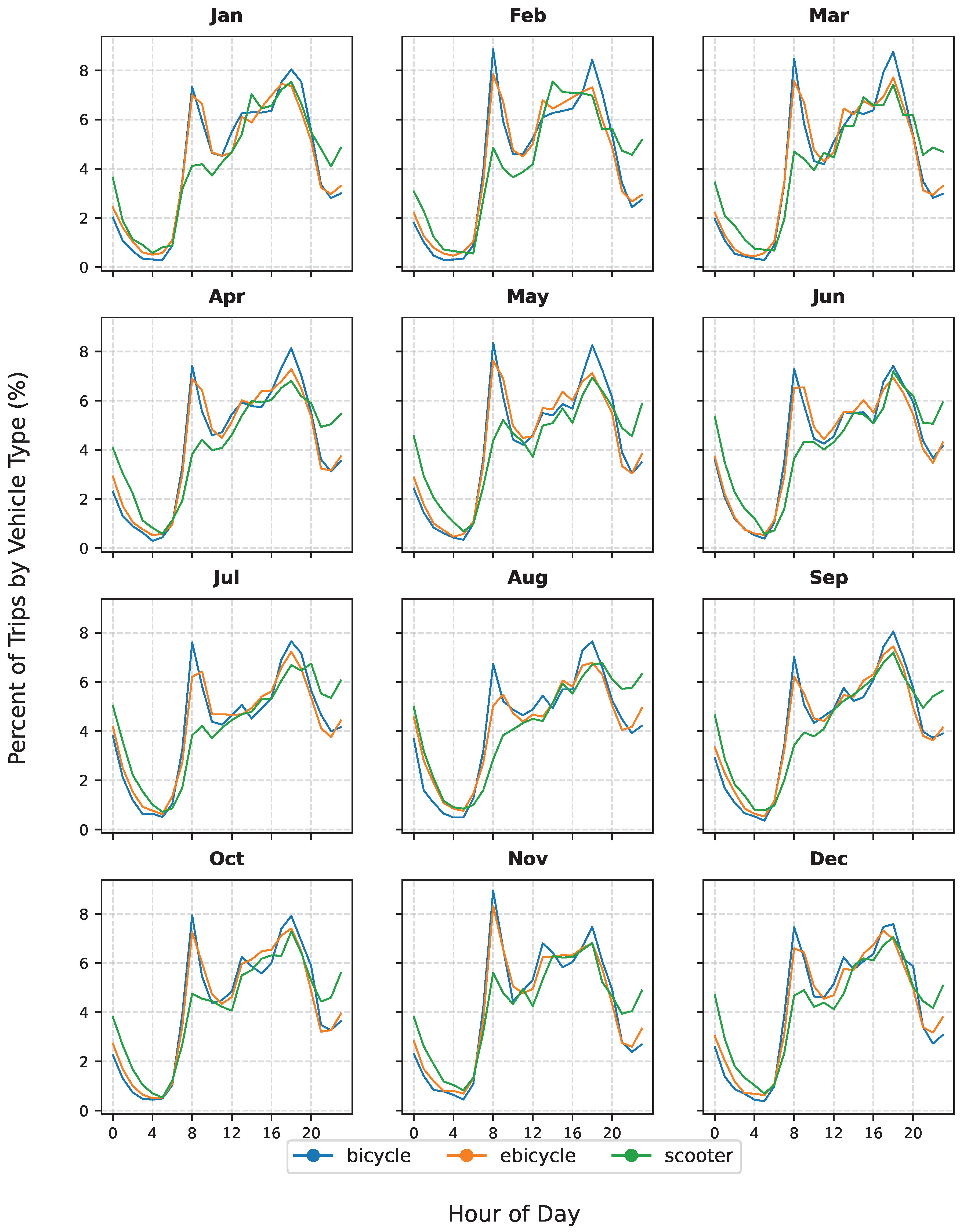
Figure A2.
Florence monthly average daily demand pattern of weekends (Saturday-Sunday) for all modes. e-bikes displayed in orange, bikes in blue, e-scooters in green.
Figure A2.
Florence monthly average daily demand pattern of weekends (Saturday-Sunday) for all modes. e-bikes displayed in orange, bikes in blue, e-scooters in green.
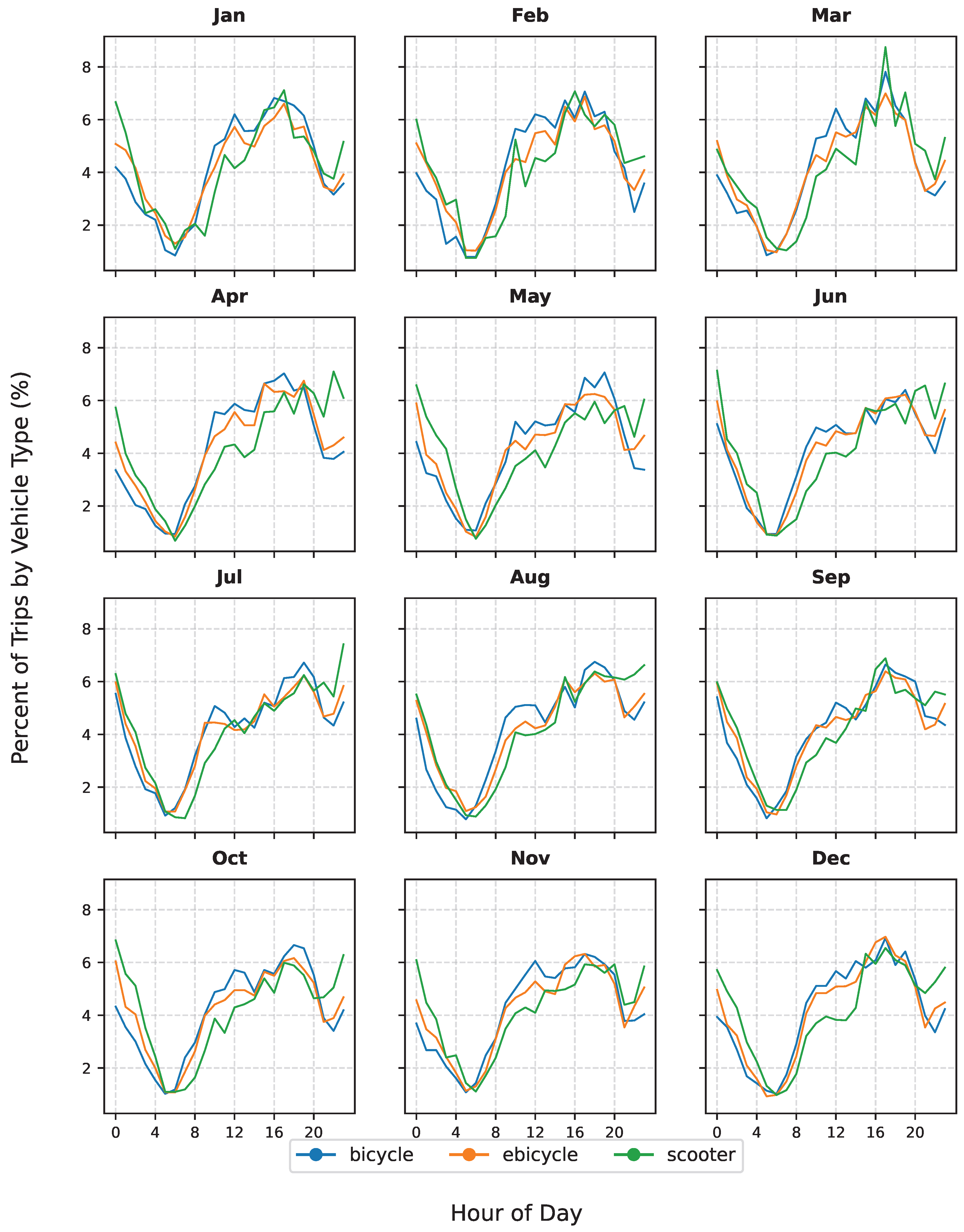
Figure A3.
Bologna monthly average daily demand pattern of working days (Monday-Friday) for all modes. E-bikes displayed in orange, bikes in blue.
Figure A3.
Bologna monthly average daily demand pattern of working days (Monday-Friday) for all modes. E-bikes displayed in orange, bikes in blue.
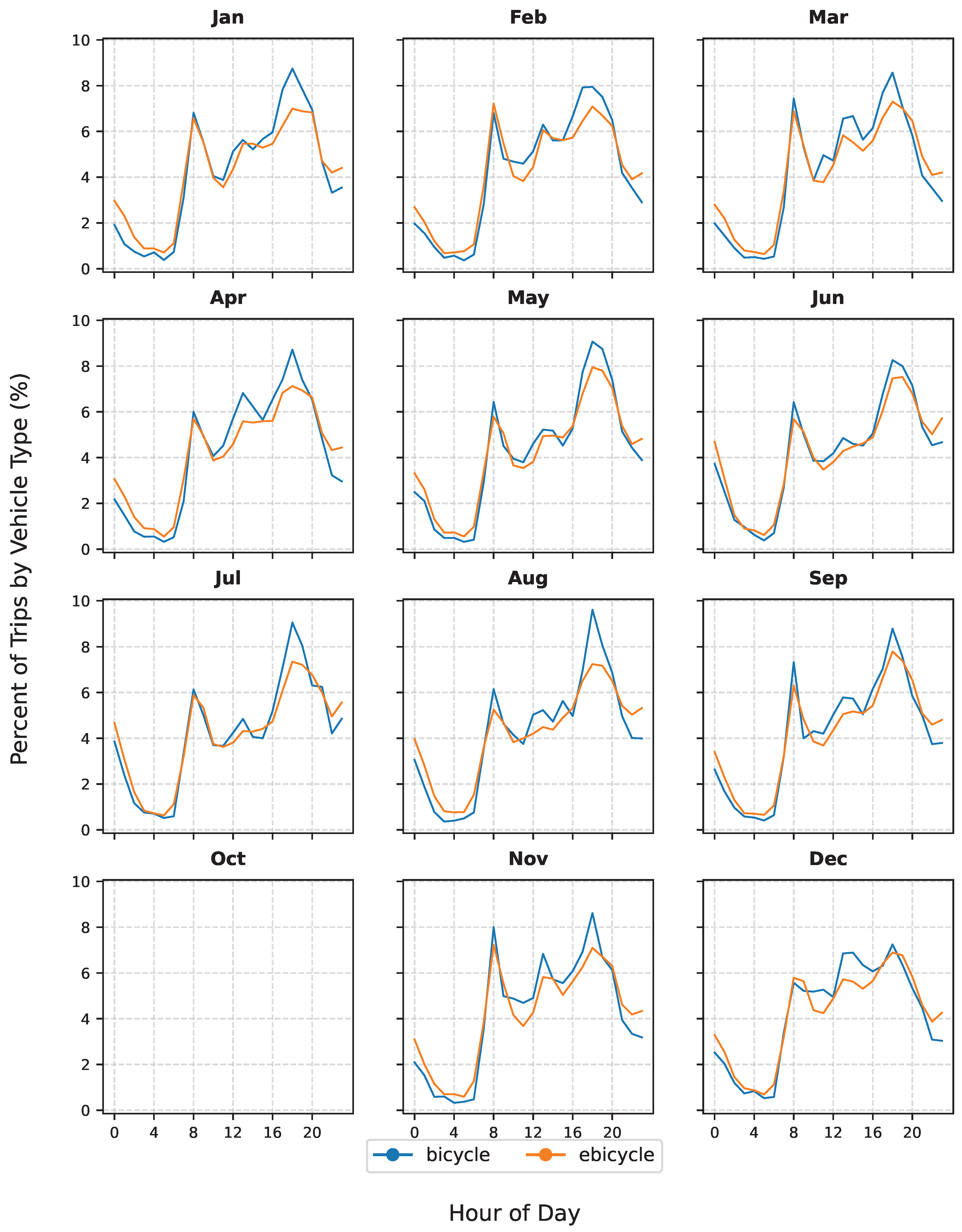
Figure A4.
Bologna monthly average daily demand pattern of weekends (Saturday-Sunday) for all modes. E-bikes displayed in orange, bikes in blue.
Figure A4.
Bologna monthly average daily demand pattern of weekends (Saturday-Sunday) for all modes. E-bikes displayed in orange, bikes in blue.
References
- Li, W.; Kamargianni, M. Providing quantified evidence to policy makers for promoting bike-sharing in heavily air-polluted cities: A mode choice model and policy simulation for Taiyuan-China. Transportation research part A: policy and practice 2018, 111, 277–291. [Google Scholar] [CrossRef]
- Agency, E.E. SOER 2020 Executive SUmmary, 2020. Last accessed 9 August 2025.
- Zhang, Y.; Mi, Z. Environmental benefits of bike sharing: A big data-based analysis. Applied energy 2018, 220, 296–301. [Google Scholar] [CrossRef]
- Buehler, R.; Hamre, A.; et al. Economic benefits of capital bikeshare: A focus on users and businesses. Technical report, Mid-Atlantic Universities Transportation Center, 2014.
- Milne, A.; Melin, M. Bicycling and walking in the United States: 2014 benchmarking report 2014.
- Bauman, A.; Crane, M.; Drayton, B.A.; Titze, S. The unrealised potential of bike share schemes to influence population physical activity levels–A narrative review. Preventive medicine 2017, 103, S7–S14. [Google Scholar] [CrossRef] [PubMed]
- Eren, E.; Uz, V.E. A review on bike-sharing: The factors affecting bike-sharing demand. Sustainable cities and society 2020, 54, 101882. [Google Scholar] [CrossRef]
- Teixeira, J.F.; Silva, C.; Moura e Sá, F. Empirical evidence on the impacts of bikesharing: a literature review. Transport reviews 2021, 41, 329–351. [Google Scholar] [CrossRef]
- Li, Q.; Luca, D.; Fuerst, F.; Wei, Z. Success in tandem? The impact of the introduction of e-bike sharing on bike sharing usage. Research in Transportation Economics 2024, 107, 101476. [Google Scholar] [CrossRef]
- fka Andersson, A.S.; Adell, E.; Hiselius, L.W. What is the substitution effect of e-bikes? A randomised controlled trial. Transportation research part D: transport and environment 2021, 90, 102648. [Google Scholar] [CrossRef]
- Campbell, A.A.; Cherry, C.R.; Ryerson, M.S.; Yang, X. Factors influencing the choice of shared bicycles and shared electric bikes in Beijing. Transportation research part C: emerging technologies 2016, 67, 399–414. [Google Scholar] [CrossRef]
- Mafi, S.; McIntyre, E.; Prior, J.; Mohammadi, A.; Choobchian, P. Riding together: A scoping review of factors influencing user behaviour in bike-sharing systems. Transportation Research Part F: Traffic Psychology and Behaviour 2026, 116, 103413. [Google Scholar] [CrossRef]
- Hyland, M.; Hong, Z.; de Farias Pinto, H.K.R.; Chen, Y. Hybrid cluster-regression approach to model bikeshare station usage. Transportation Research Part A: Policy and Practice 2018, 115, 71–89. [Google Scholar] [CrossRef]
- Kim, K. Investigation on the effects of weather and calendar events on bike-sharing according to the trip patterns of bike rentals of stations. Journal of transport geography 2018, 66, 309–320. [Google Scholar] [CrossRef]
- Reiss, S.; Bogenberger, K. Validation of a relocation strategy for Munich’s bike sharing system. Transportation Research Procedia 2016, 19, 341–349. [Google Scholar] [CrossRef]
- Gallop, C.; Tse, C.; Zhao, J. A seasonal autoregressive model of Vancouver bicycle traffic using weather variables. In Proceedings of the Transportation research board 91st annual meeting, 2012, number 12-2119.
- Schoner, J.E.; Levinson, D.M. The missing link: Bicycle infrastructure networks and ridership in 74 US cities. Transportation 2014, 41, 1187–1204. [Google Scholar] [CrossRef]
- Habib, K.N.; Mann, J.; Mahmoud, M.; Weiss, A. Synopsis of bicycle demand in the City of Toronto: Investigating the effects of perception, consciousness and comfortability on the purpose of biking and bike ownership. Transportation research part A: policy and practice 2014, 70, 67–80. [Google Scholar] [CrossRef]
- Lu, W.; Scott, D.M.; Dalumpines, R. Understanding bike share cyclist route choice using GPS data: Comparing dominant routes and shortest paths. Journal of transport geography 2018, 71, 172–181. [Google Scholar] [CrossRef]
- Kabak, M.; Erbaş, M.; Çetinkaya, C.; Özceylan, E. A GIS-based MCDM approach for the evaluation of bike-share stations. Journal of cleaner production 2018, 201, 49–60. [Google Scholar] [CrossRef]
- Kaltenbrunner, A.; Meza, R.; Grivolla, J.; Codina, J.; Banchs, R. Urban cycles and mobility patterns: Exploring and predicting trends in a bicycle-based public transport system. Pervasive and Mobile Computing 2010, 6, 455–466. [Google Scholar] [CrossRef]
- Wang, K.; Akar, G.; Chen, Y.J. Bike sharing differences among millennials, Gen Xers, and baby boomers: Lessons learnt from New York City’s bike share. Transportation research part A: policy and practice 2018, 116, 1–14. [Google Scholar] [CrossRef]
- Feng, P.; Li, W. Willingness to use a public bicycle system: An example in Nanjing City. Journal of Public Transportation 2016, 19, 84–96. [Google Scholar] [CrossRef]
- Fishman, E.; Washington, S.; Haworth, N. Bike share’s impact on car use: Evidence from the United States, Great Britain, and Australia. Transportation research part D: transport and environment 2014, 31, 13–20. [Google Scholar] [CrossRef]
- Ricci, M. Bike sharing: A review of evidence on impacts and processes of implementation and operation. Research in Transportation Business & Management 2015, 15, 28–38. [Google Scholar] [CrossRef]
- Martin, E.; Shaheen, S.; Cohen, A. Public Bikesharing in North America: Early Operator and User Understanding, 2013.
- Mobility, O.N.S. Ottavo rapporto nazionale sulla sharing mobility, 2024.
- Chun, B.; Nguyen, A.; Pan, Q.; Mirzaaghazadeh, E. Spatial Analysis of bike-sharing ridership for sustainable transportation in Houston, Texas. Sustainability 2024, 16, 2569. [Google Scholar] [CrossRef]
- Jin, S.T.; Sui, D.Z. A comparative analysis of the spatial determinants of e-bike and e-scooter sharing link flows. Journal of Transport Geography 2024, 119, 103959. [Google Scholar] [CrossRef]
- Zhou, X. Understanding spatiotemporal patterns of biking behavior by analyzing massive bike sharing data in Chicago. PloS one 2015, 10, e0137922. [Google Scholar] [CrossRef]
- Zhao, J.; Wang, J.; Deng, W. Exploring bikesharing travel time and trip chain by gender and day of the week. Transportation Research Part C: Emerging Technologies 2015, 58, 251–264. [Google Scholar] [CrossRef]
- Chung, J.; Yao, E.; Ko, J.; Namkung, O.S. Investigation of private and public bikes usage patterns considering GPS trajectory based cycling features. Journal of Transport Geography 2024, 118, 103904. [Google Scholar] [CrossRef]
- Berke, A.; Truitt, W.; Larson, K. Is access to public bike-share networks equitable? A multiyear spatial analysis across 5 US Cities. Journal of transport geography 2024, 114, 103759. [Google Scholar] [CrossRef]
- Shang, W.L.; Chen, J.; Bi, H.; Sui, Y.; Chen, Y.; Yu, H. Impacts of COVID-19 pandemic on user behaviors and environmental benefits of bike sharing: A big-data analysis. Applied Energy 2021, 285, 116429. [Google Scholar] [CrossRef]
- Diao, M.; Song, K.; Shi, S.; Zhu, Y.; Liu, B. The environmental benefits of dockless bike sharing systems for commuting trips. Transportation research part D: transport and environment 2023, 124, 103959. [Google Scholar] [CrossRef]
- Bhowmick, D.; Dai, D.; Saberi, M.; Nelson, T.; Stevenson, M.; Seneviratne, S.; Nice, K.; Pettit, C.; Vu, H.L.; Beck, B. Collecting population-representative bike-riding GPS data to understand bike-riding activity and patterns using smartphones and Bluetooth beacons. Travel Behaviour and Society 2025, 38, 100919. [Google Scholar] [CrossRef]
- Schweizer, J. Sumopy: an advanced simulation suite for sumo. In Proceedings of the Simulation of Urban MObility User Conference; Springer, 2013; pp. 71–82. [Google Scholar]
- Schweizer, J.; Schuhmann, F.; Poliziani, C. hybridPy: The Simulation Suite for Mesoscopic and Microscopic Traffic Simulations. In Proceedings of the SUMO Conference Proceedings; 2024; Vol. 5, pp. 39–55. [Google Scholar]
- Schweizer, J.; Rupi, F.; Poliziani, C. Estimation of link-cost function for cyclists based on stochastic optimisation and GPS traces. IET Intelligent Transport Systems 2020, 14, 1810–1814. [Google Scholar] [CrossRef]
- Turistici, C.S. La Gestione del Turismo nel Centro Storico di Firenze Patrimonio Mondiale UNESCO, 2024.
- Bernieri, G.; Rupi, F.; Schweizer, J. It’s How You Build Them: The Evolution of Cycling Infrastructure and Traffic in Bologna before and after COVID-19. Preprints 2025. [Google Scholar] [CrossRef]
- Meloni, I.; Musolino, G.; Piras, F.; Rindone, C.; Russo, F.; Sottile, E.; Vitetta, A. Mobility as a Service: Insights from pilot studies across different Italian settings. Transportation Engineering 2024, 18, 100294. [Google Scholar] [CrossRef]
- Rupi, F.; Poliziani, C.; Schweizer, J. Analysing the dynamic performances of a bicycle network with a temporal analysis of GPS traces. Case studies on transport policy 2020, 8, 770–777. [Google Scholar] [CrossRef]
- Rupi, F.; Poliziani, C.; Schweizer, J. Data-driven bicycle network analysis based on traditional counting methods and GPS traces from smartphone. ISPRS International Journal of Geo-Information 2019, 8, 322. [Google Scholar] [CrossRef]
- Ul-Abdin, Z.; Rajper, S.Z.; Schotte, K.; De Winne, P.; De Backer, H. Analytical geometric design of bicycle paths. In Proceedings of the Proceedings of the Institution of Civil Engineers-Transport; Thomas Telford Ltd., 2020; Vol. 173, pp. 361–379. [Google Scholar]
- Lyubenov, D.; Balbuzanov, T.; Steliyanov, M.; Topchu, D. Study of Main Traffic Parameters and Bicycle Path Suitability for Electric Vehicles and Bicycles in the City of Ruse. In Proceedings of the 2023 4th International Conference on Communications, Information, Electronic and Energy Systems (CIEES); IEEE, 2023; pp. 1–4. [Google Scholar]
- Paulsen, M.; Rasmussen, T.K.; Nielsen, O.A. Fast or forced to follow: A speed heterogeneous approach to congested multi-lane bicycle traffic simulation. Transportation research part B: methodological 2019, 127, 72–98. [Google Scholar] [CrossRef]
- Schleinitz, K.; Petzoldt, T.; Franke-Bartholdt, L.; Krems, J.; Gehlert, T. The German Naturalistic Cycling Study–Comparing cycling speed of riders of different e-bikes and conventional bicycles. Safety science 2017, 92, 290–297. [Google Scholar] [CrossRef]
- Waldner, F.; Balke, G.; Rech, F.; Lellep, M. Data-driven insights into (E-) bike-sharing: mining a large-scale dataset on usage and urban characteristics: descriptive analysis and performance modeling. Transportation 2025, 1–41. [Google Scholar] [CrossRef]
- Li, A.; Zhao, P.; Liu, X.; Mansourian, A.; Axhausen, K.W.; Qu, X. Comprehensive comparison of e-scooter sharing mobility: Evidence from 30 European cities. Transportation Research Part D: Transport and Environment 2022, 105, 103229. [Google Scholar] [CrossRef]
- O’brien, O.; Cheshire, J.; Batty, M. Mining bicycle sharing data for generating insights into sustainable transport systems. Journal of Transport Geography 2014, 34, 262–273. [Google Scholar] [CrossRef]
Figure 1.
Process diagram from origin-destination GPS dataset to reconstruct trips.
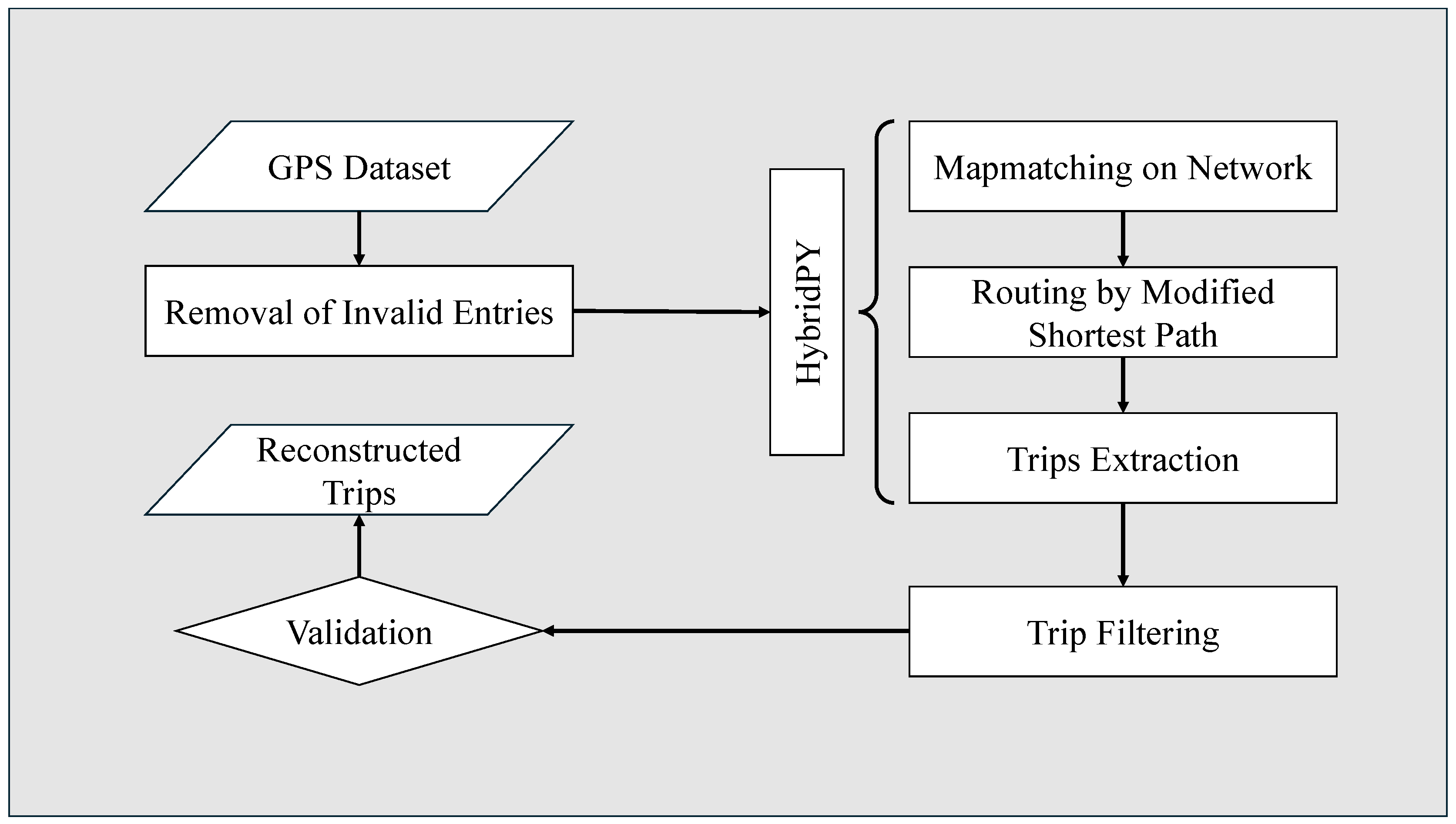
Figure 3.
From left to right: total trips in 2023, unique vehicle IDs in 2023: e-bikes displayed in orange, bikes in blue, e-scooters in green, city of Florence.
Figure 3.
From left to right: total trips in 2023, unique vehicle IDs in 2023: e-bikes displayed in orange, bikes in blue, e-scooters in green, city of Florence.
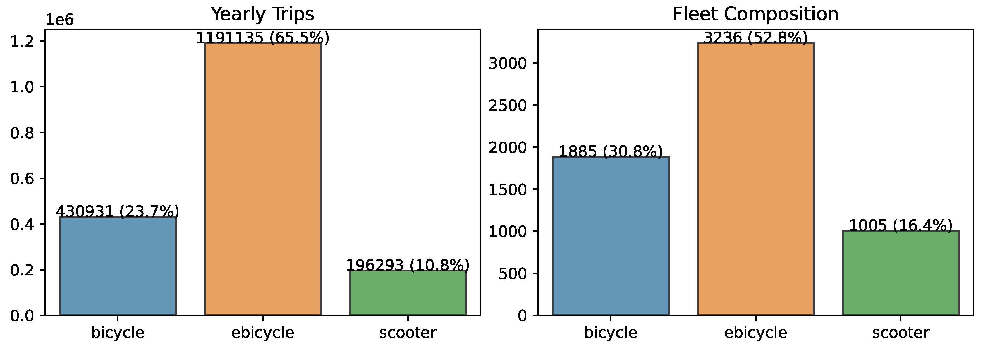
Figure 4.
Trip parameter distributions (post-filtering) for all modes in Florence. From top to bottom: trip length (meters), average trip speed (meters per second), and trip duration (seconds). E-bikes in orange, bikes in blue, and e-scooters in green.
Figure 4.
Trip parameter distributions (post-filtering) for all modes in Florence. From top to bottom: trip length (meters), average trip speed (meters per second), and trip duration (seconds). E-bikes in orange, bikes in blue, and e-scooters in green.
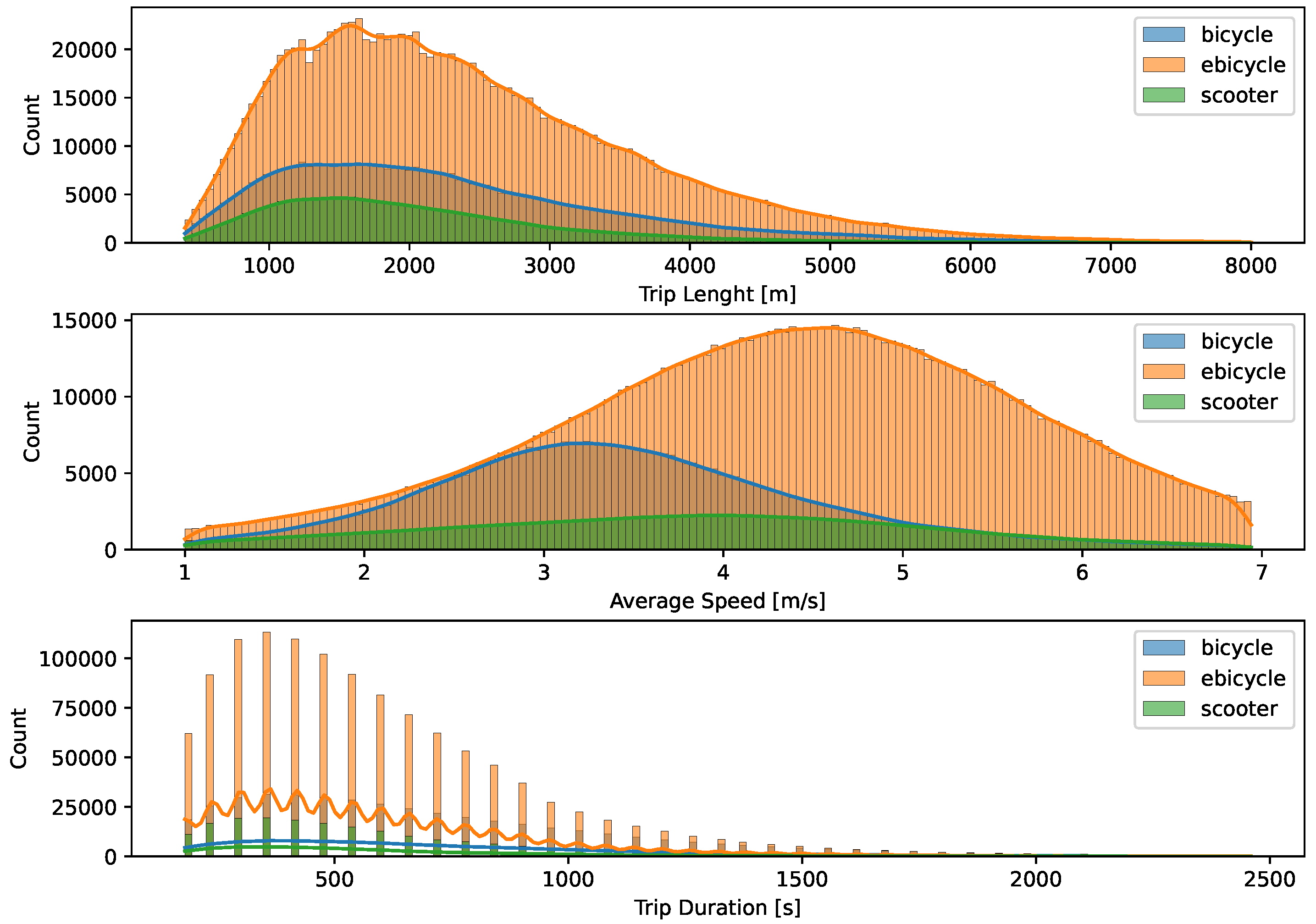
Figure 5.
(a) Heatmap of Florence trips’ origins. (b) Heatmap of Florence trips’ destinations. (c) Heatmap of Florence net yearly flows in the 250x250 meters cells. Negative values indicate that in that cell more trips started than ended, indicating a deficit of bikes in that area throughout the year. Positive values, in red, indicate that in that cell more trips ended than started, indicating a surplus of bikes in that area throughout the year.
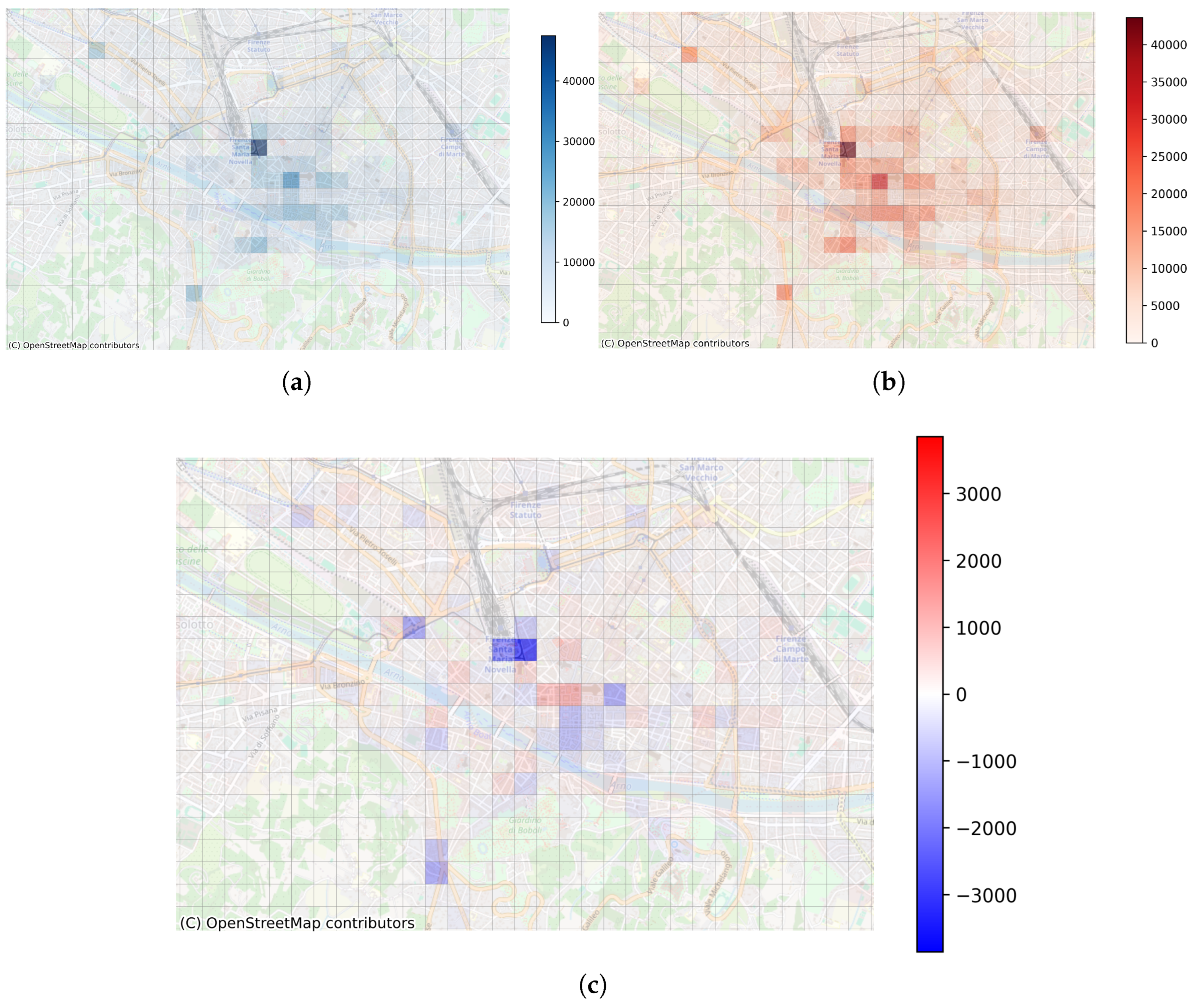
Figure 6.
Month-by-month variation of trips, average daily turnover, and fleet composition in Florence. E-bikes displayed in orange, bikes in blue, e-scooters in green.
Figure 6.
Month-by-month variation of trips, average daily turnover, and fleet composition in Florence. E-bikes displayed in orange, bikes in blue, e-scooters in green.
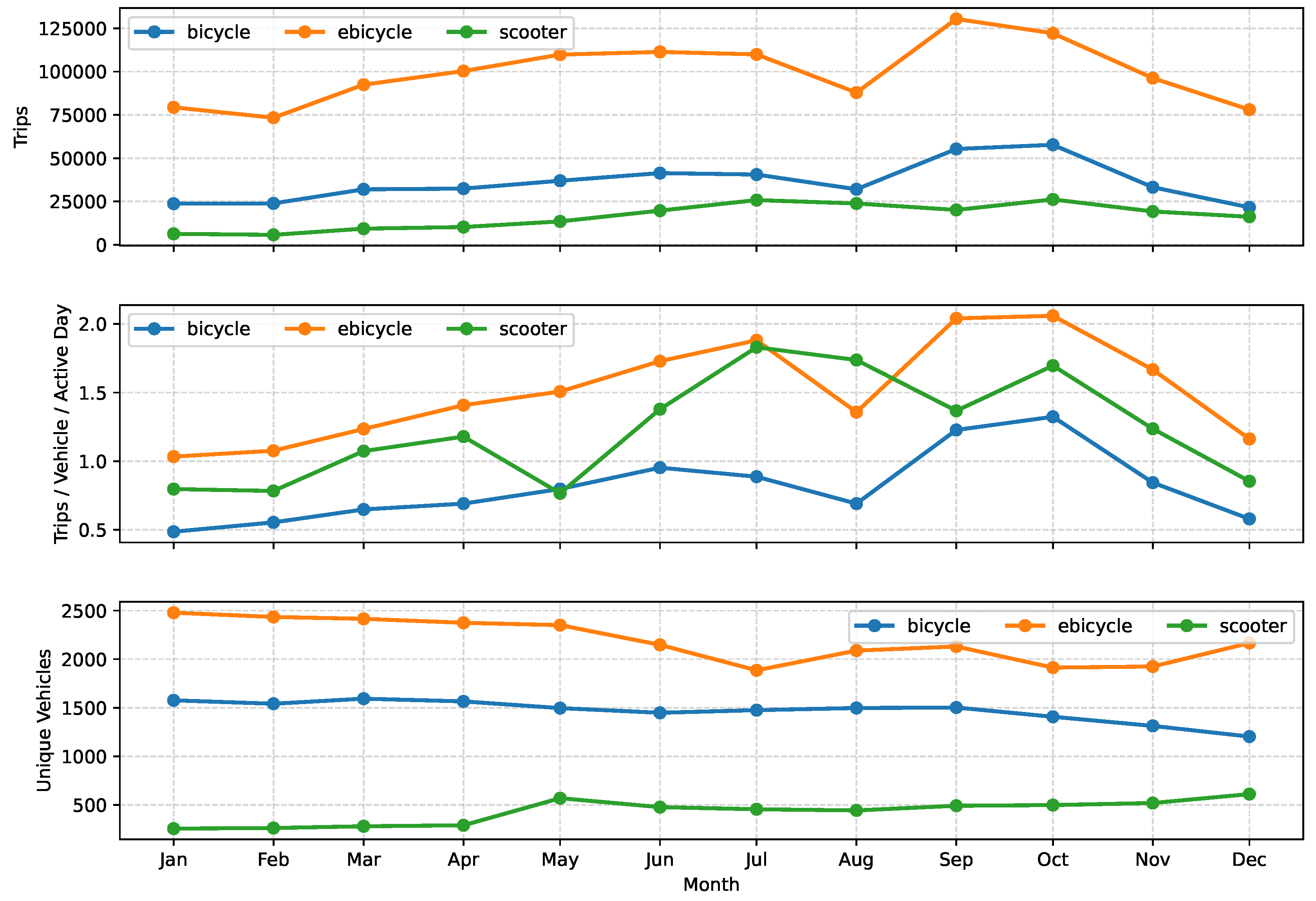
Figure 7.
Portions of the yearly average daily turnover by trip length ranges in Florence. E-bikes displayed in orange, bikes in blue, e-scooters in green.
Figure 7.
Portions of the yearly average daily turnover by trip length ranges in Florence. E-bikes displayed in orange, bikes in blue, e-scooters in green.
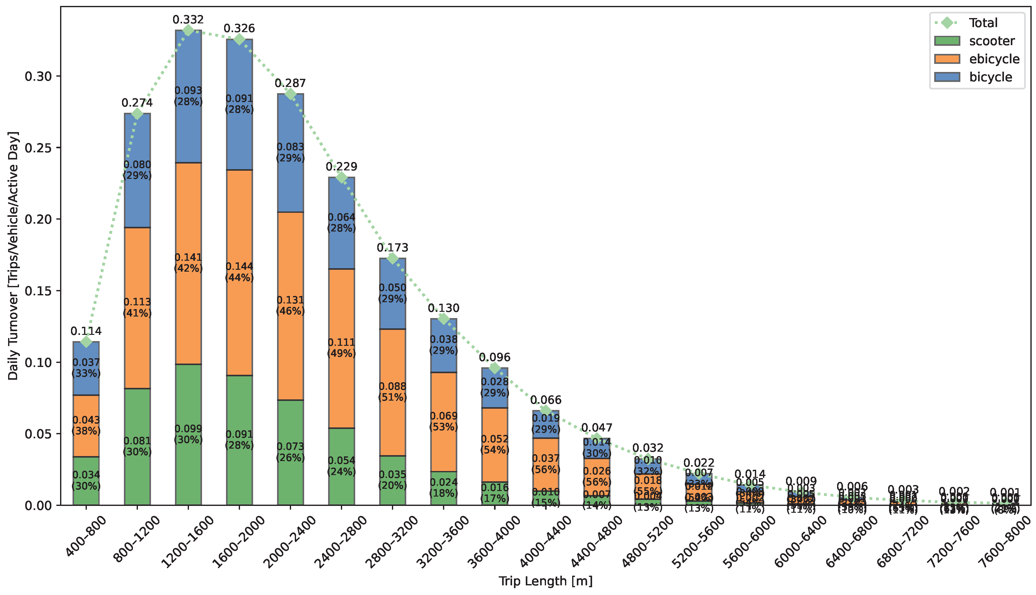
Figure 8.
Distributions of trip length, average speed, and trip duration on different days of the week in Florence. E-bikes displayed in orange, bikes in blue, e-scooters in green.
Figure 8.
Distributions of trip length, average speed, and trip duration on different days of the week in Florence. E-bikes displayed in orange, bikes in blue, e-scooters in green.
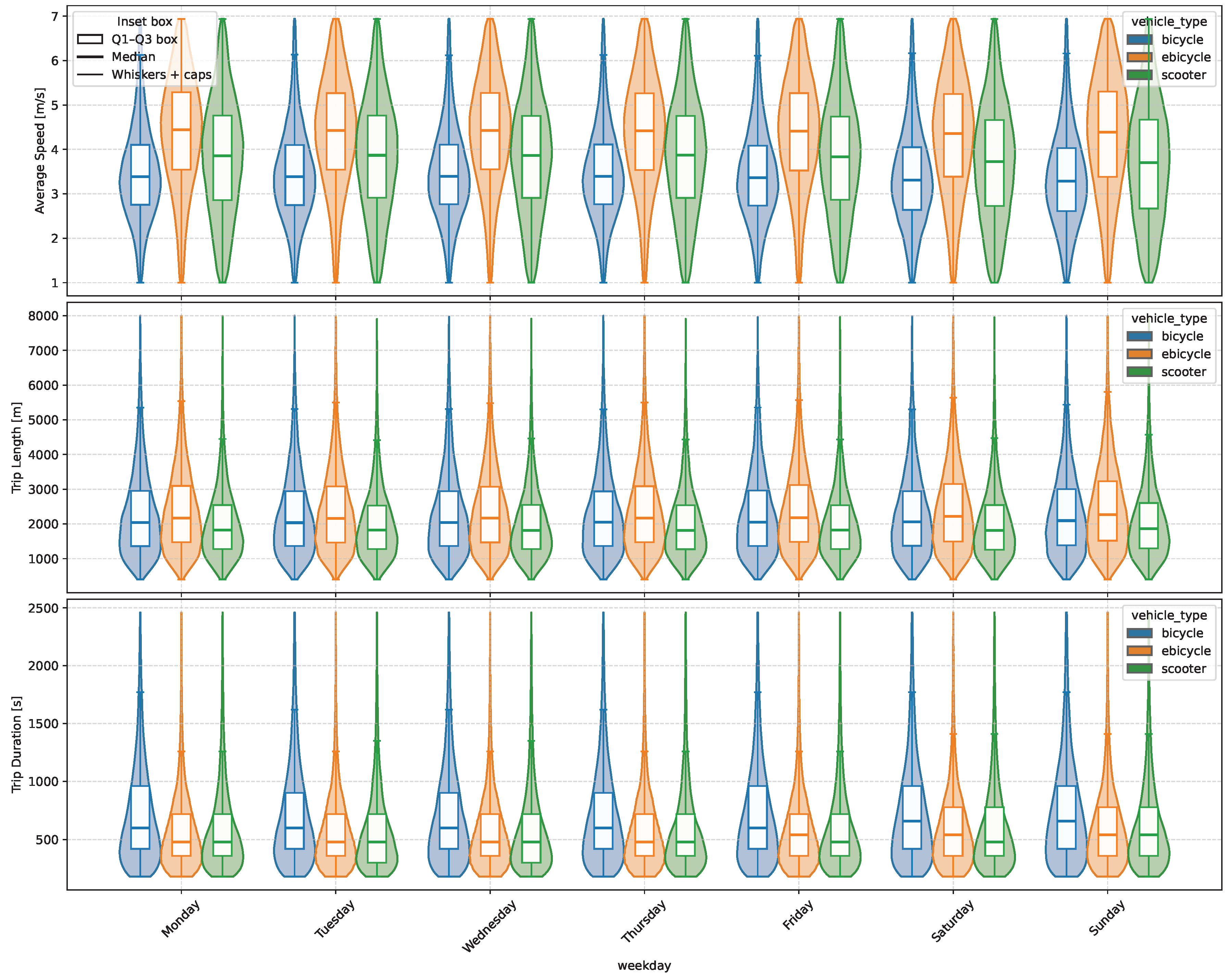
Figure 9.
Yearly average daily demand pattern of weekdays (Monday-Friday) for all modes in Florence. E-bikes displayed in orange, bikes in blue, e-scooters in green.
Figure 9.
Yearly average daily demand pattern of weekdays (Monday-Friday) for all modes in Florence. E-bikes displayed in orange, bikes in blue, e-scooters in green.
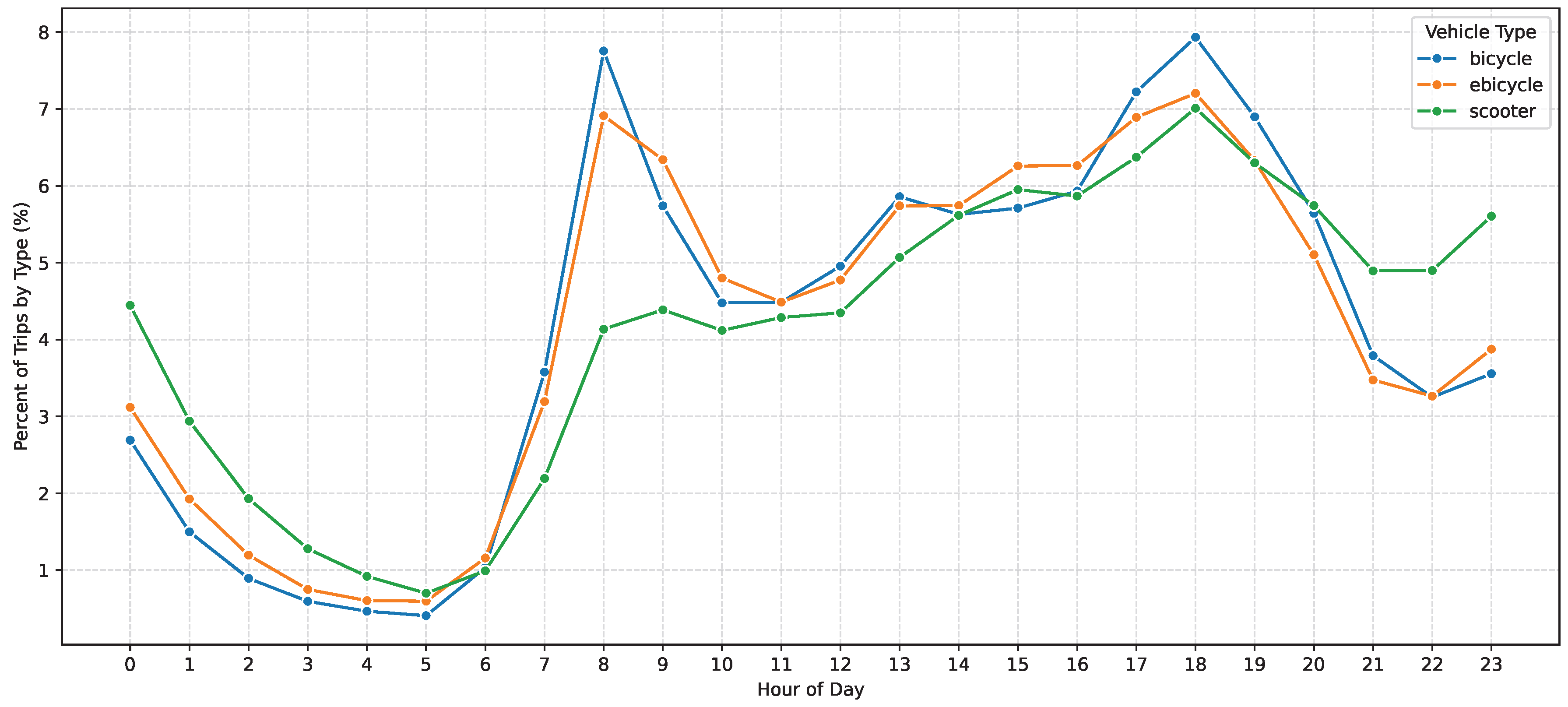
Figure 10.
Yearly average daily demand pattern of weekends (Saturday-Sunday) for all modes in Florence. E-bikes displayed in orange, bikes in blue, e-scooters in green.
Figure 10.
Yearly average daily demand pattern of weekends (Saturday-Sunday) for all modes in Florence. E-bikes displayed in orange, bikes in blue, e-scooters in green.
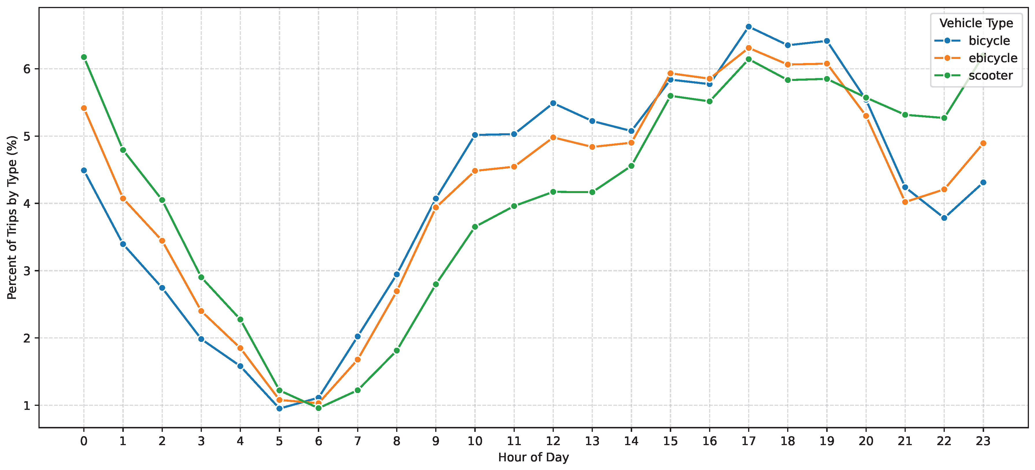
Figure 11.
From left to right: total trips in 2023, unique vehicle IDs in 2023 in Bologna. E-bikes displayed in orange, bikes in blue.
Figure 11.
From left to right: total trips in 2023, unique vehicle IDs in 2023 in Bologna. E-bikes displayed in orange, bikes in blue.
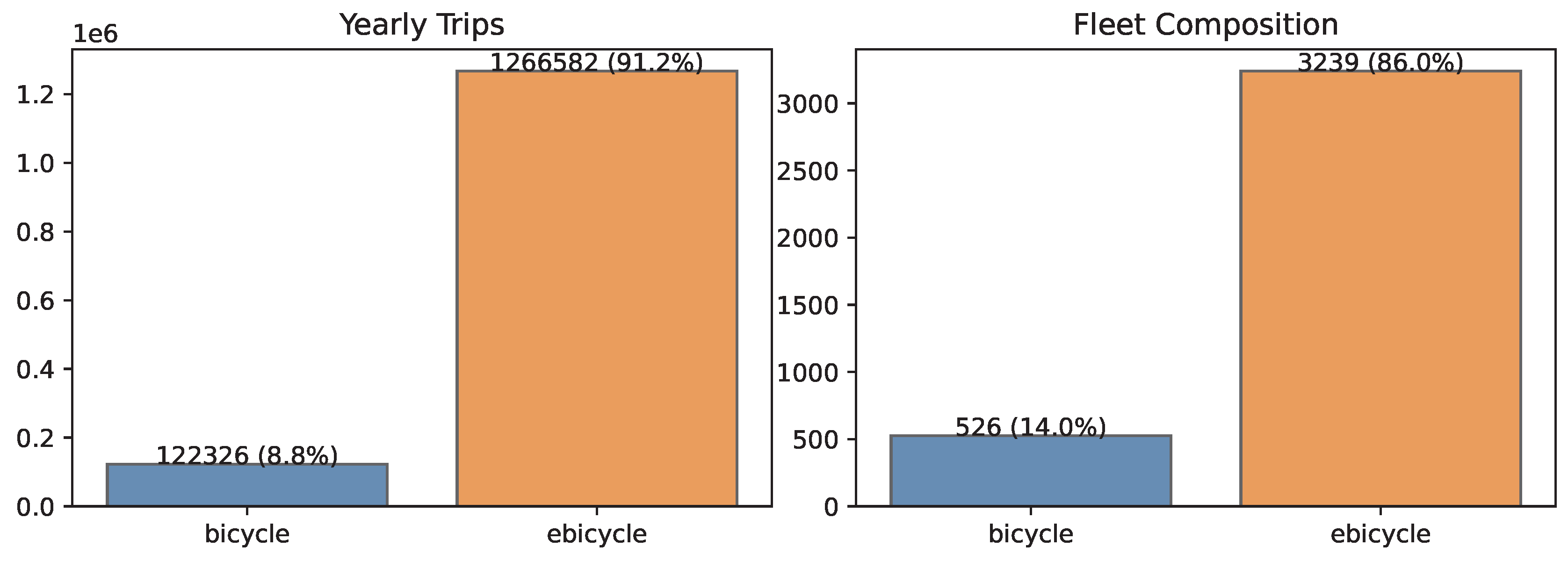
Figure 12.
Main trip parameters distribution (post-filtering) for all modes in Bologna. From top to bottom: Trip length [meters], Average trip speed [meters/second], and Trip duration [seconds]. E-bikes displayed in orange, bikes in blue.
Figure 12.
Main trip parameters distribution (post-filtering) for all modes in Bologna. From top to bottom: Trip length [meters], Average trip speed [meters/second], and Trip duration [seconds]. E-bikes displayed in orange, bikes in blue.
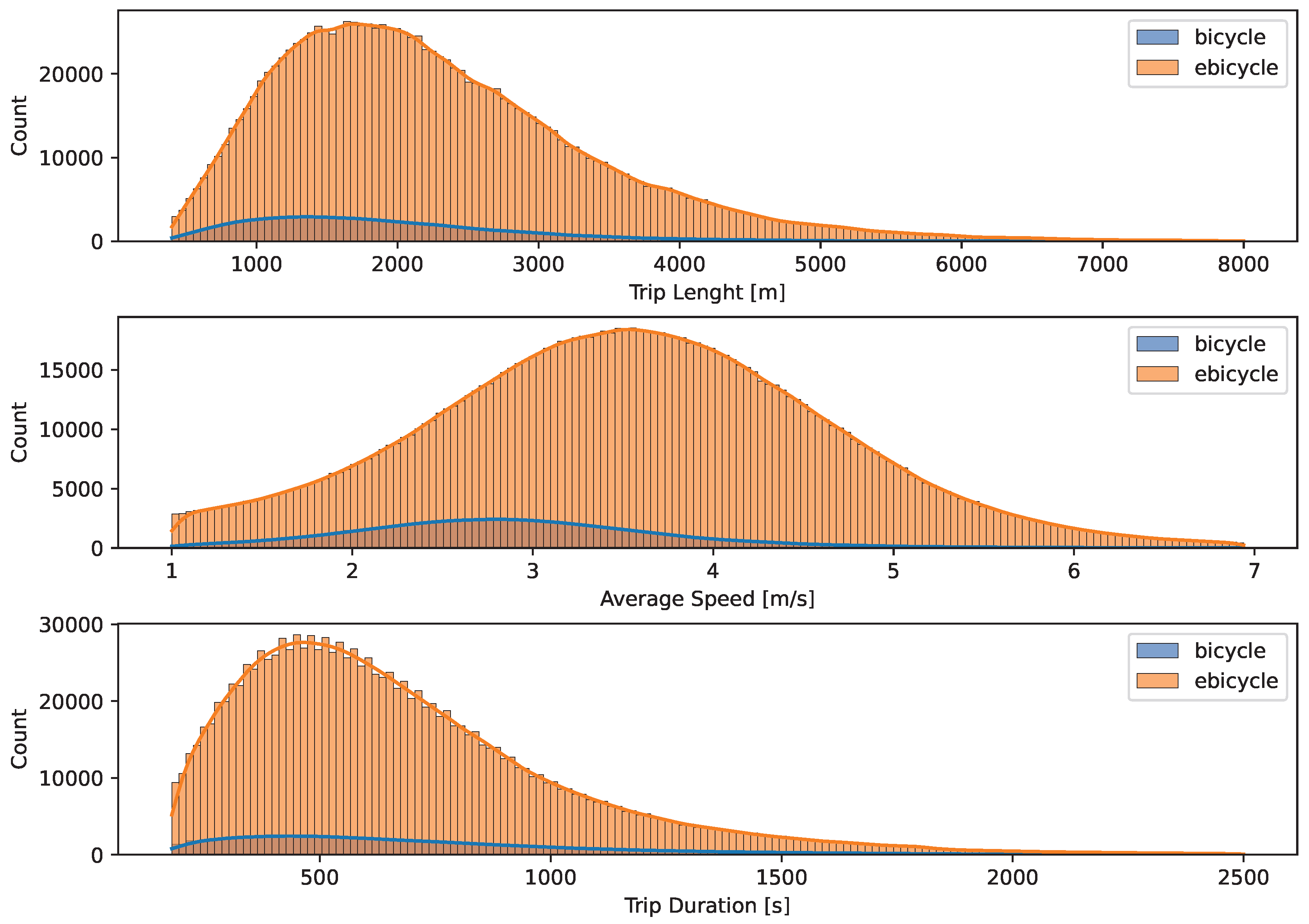
Figure 13.
(a) Heatmap of Bologna trips’ origins. (b) Heatmap of Bologna trips’ destinations. (c) Heatmap of Bologna net yearly flows in the 250x250 meters cells. Negative values indicate that in that cell more trips started than ended, indicating a deficit of bikes in that area throughout the year. Positive values, in red, indicate that in that cell more trips ended than started, indicating a surplus of bikes in that area throughout the year.
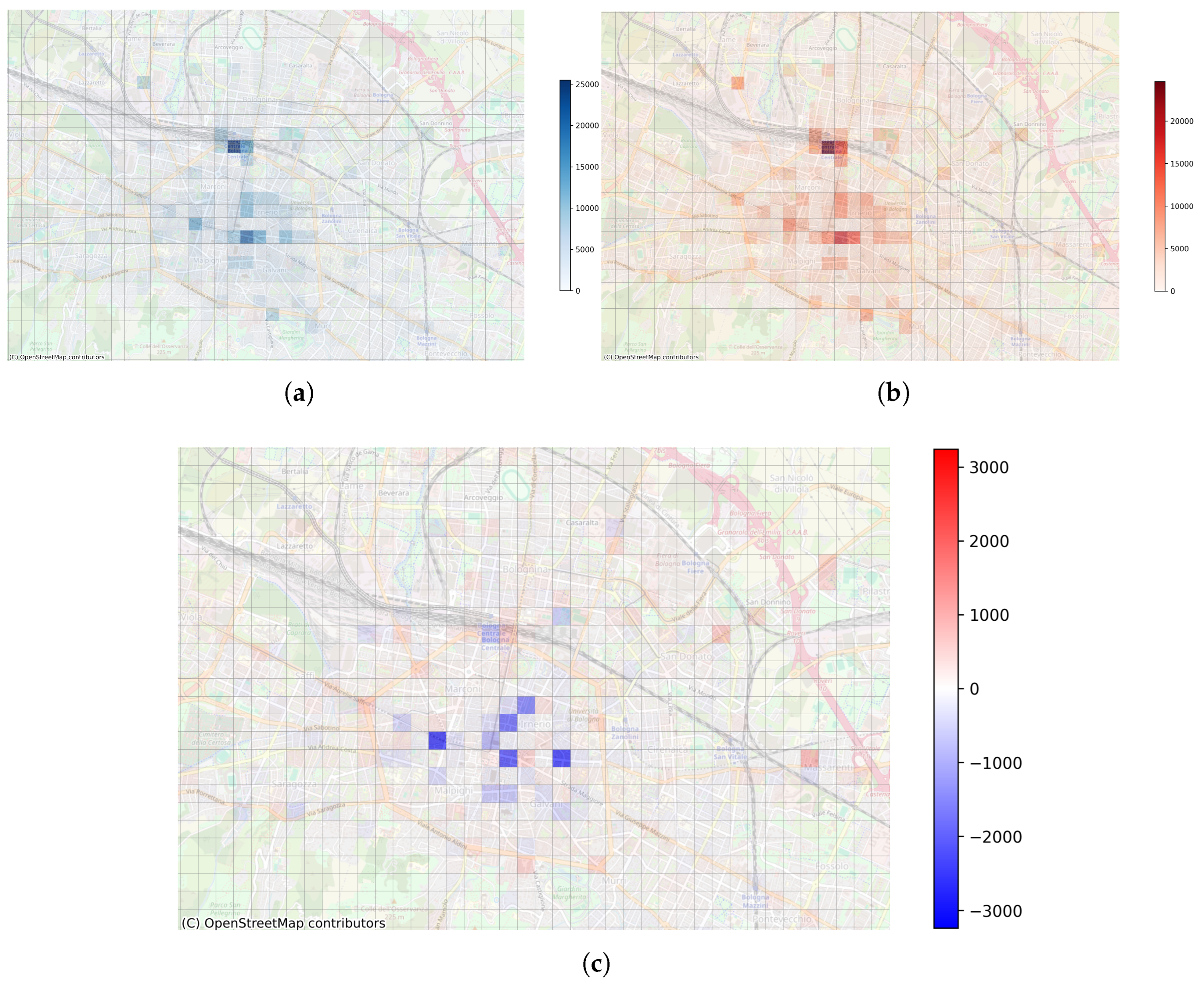
Figure 14.
Month-by-month variation of trips, average daily turnover, and fleet composition in Bologna. E-bikes displayed in orange, bikes in blue.
Figure 14.
Month-by-month variation of trips, average daily turnover, and fleet composition in Bologna. E-bikes displayed in orange, bikes in blue.
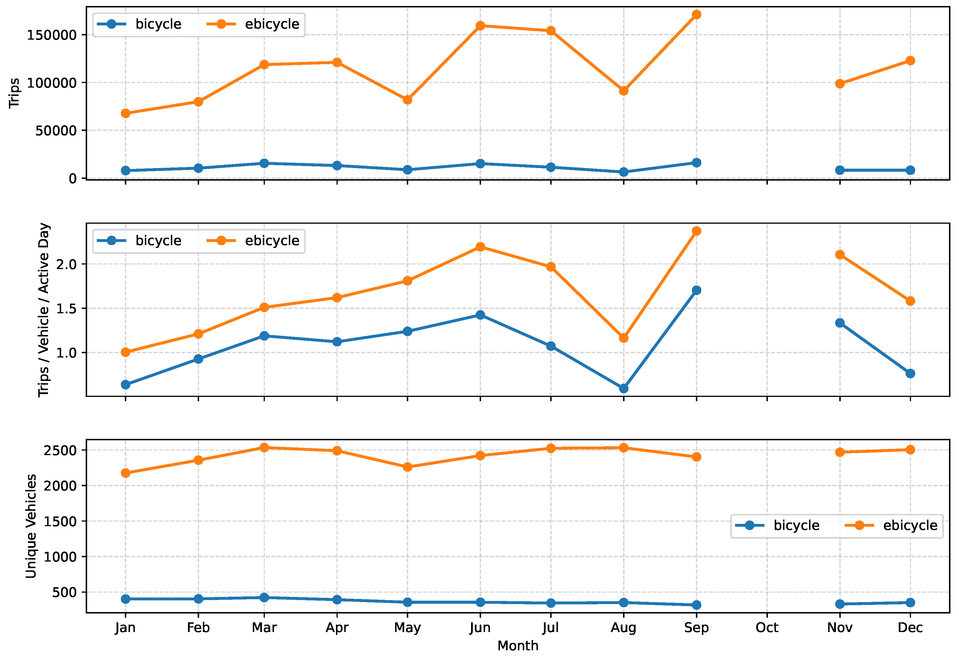
Figure 15.
Portions of yearly average daily turnover by trip length ranges in Bologna. E-bikes displayed in orange, bikes in blue.
Figure 15.
Portions of yearly average daily turnover by trip length ranges in Bologna. E-bikes displayed in orange, bikes in blue.
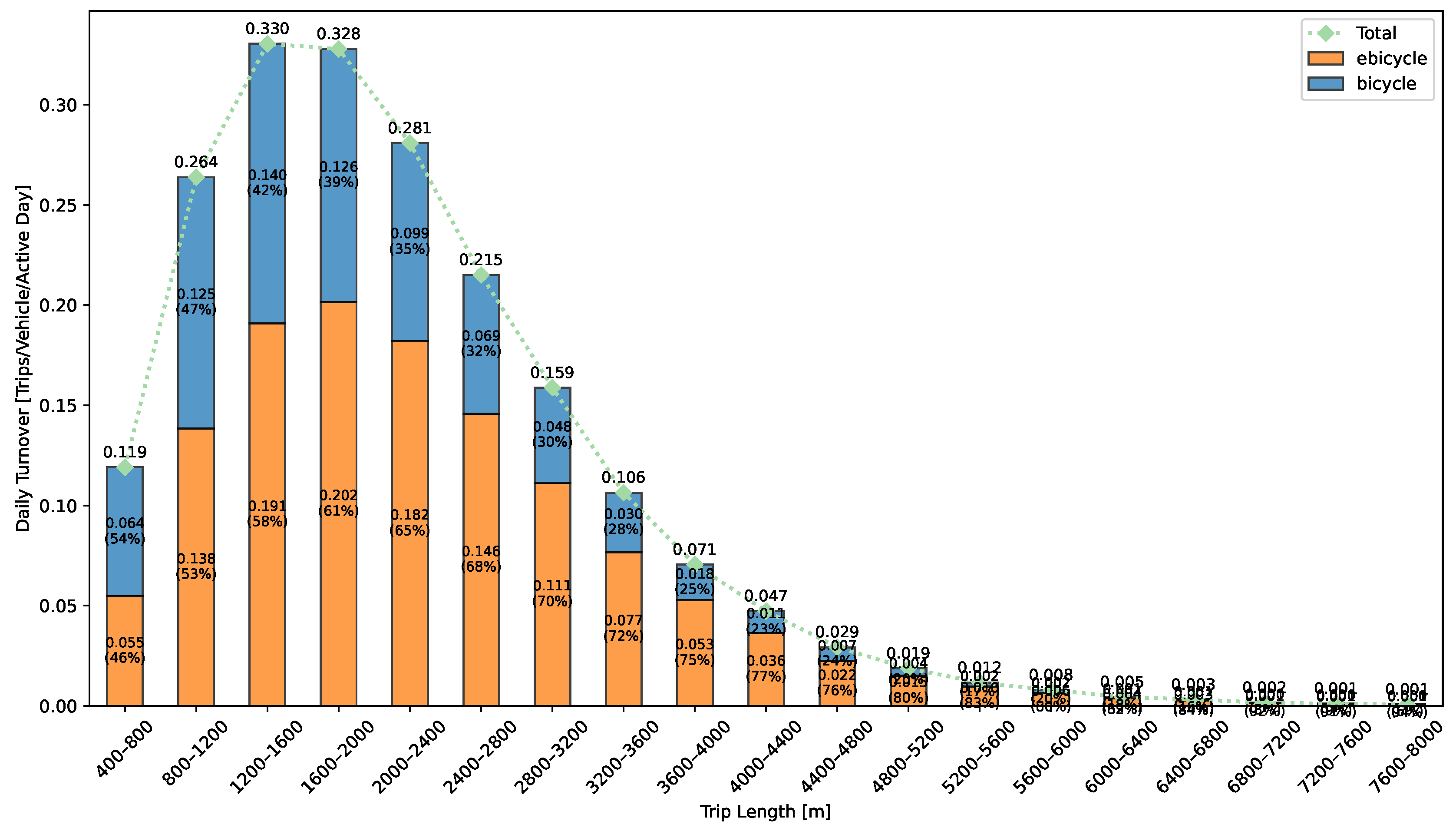
Figure 16.
Distributions of trip length, average speed, and trip duration on different days of the week in Bologna. E-bikes displayed in orange, bikes in blue.
Figure 16.
Distributions of trip length, average speed, and trip duration on different days of the week in Bologna. E-bikes displayed in orange, bikes in blue.
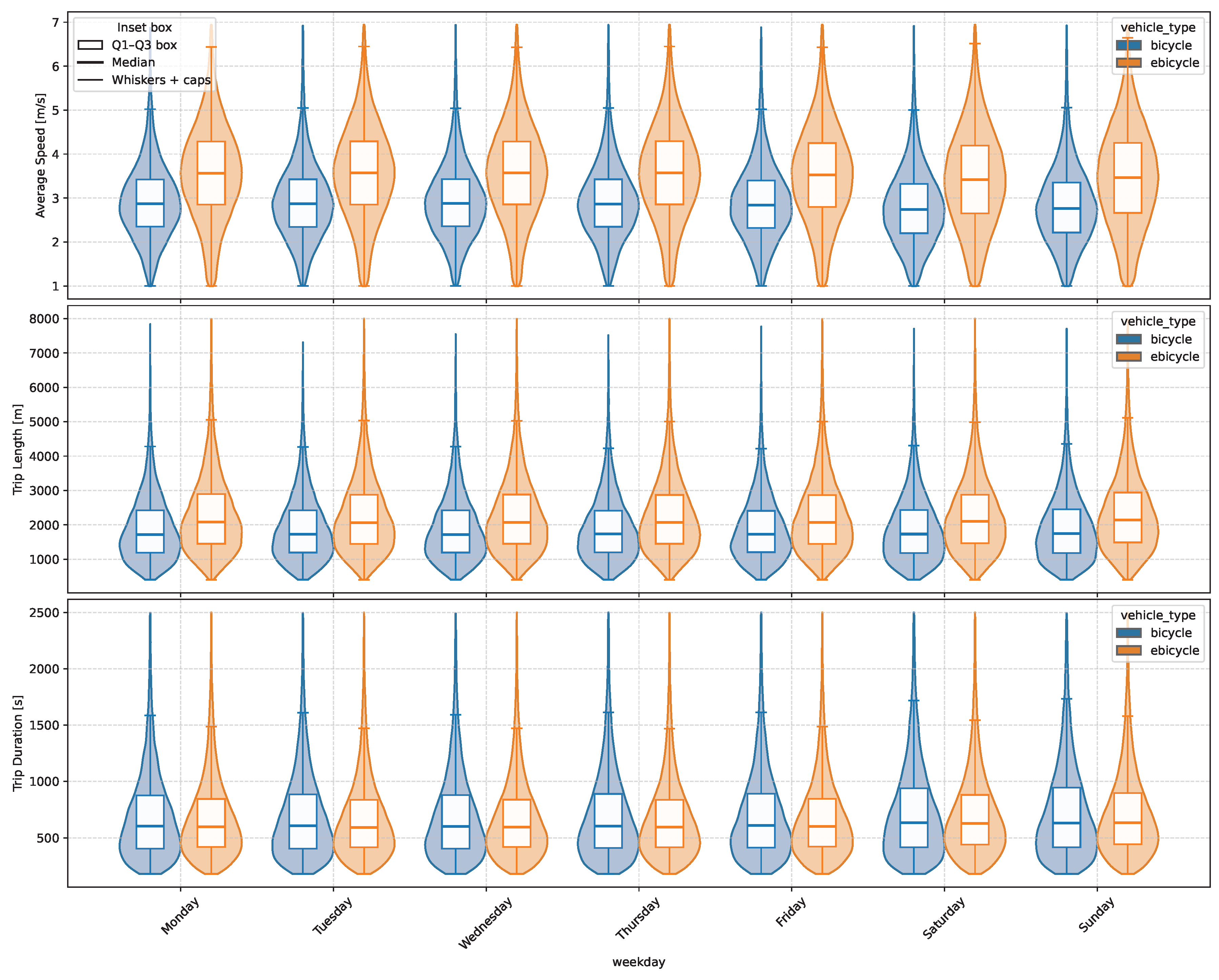
Figure 17.
Yearly average daily demand pattern of weekdays (Monday-Friday) for all modes in Bologna. E-bikes displayed in orange, bikes in blue.
Figure 17.
Yearly average daily demand pattern of weekdays (Monday-Friday) for all modes in Bologna. E-bikes displayed in orange, bikes in blue.
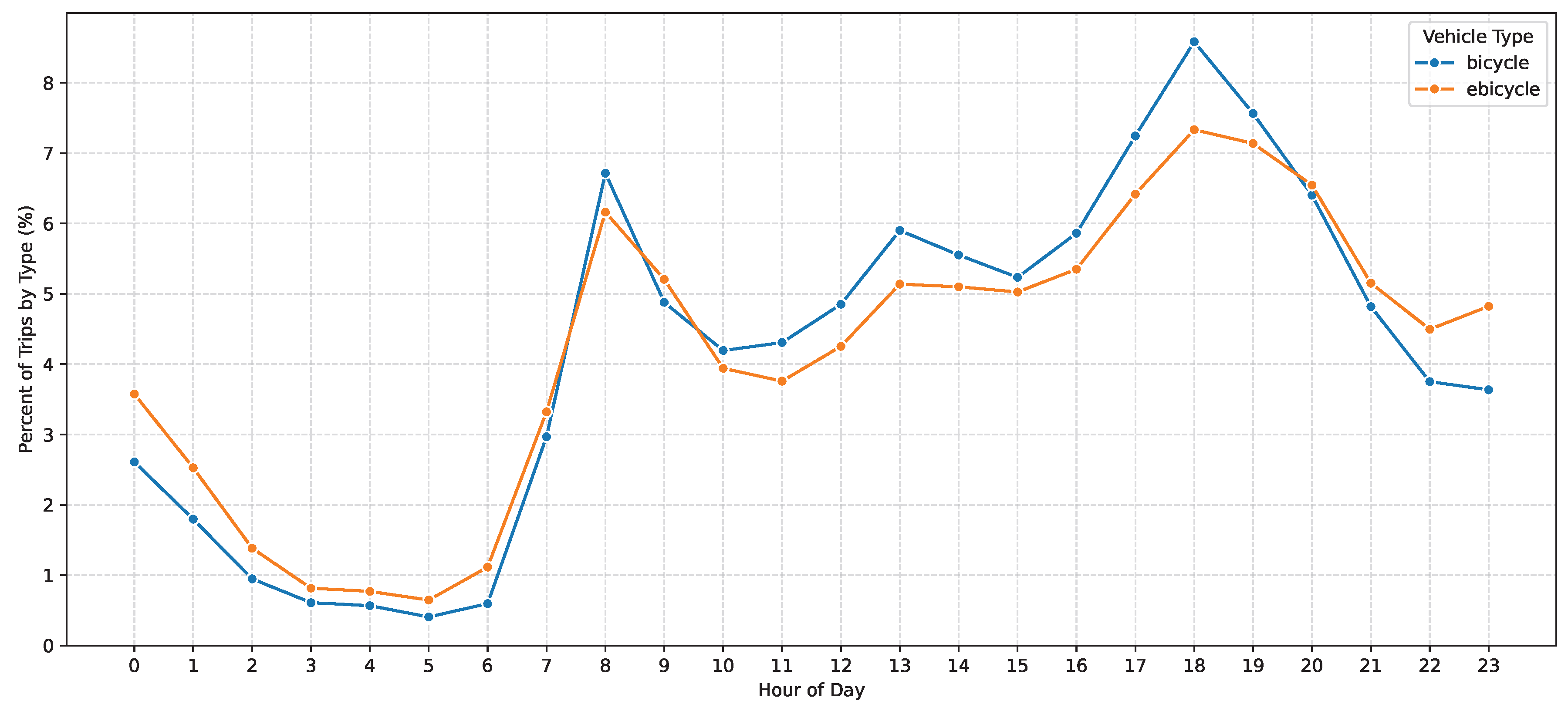
Figure 18.
Yearly average daily demand pattern of weekends (Saturday-Sunday) for all modes in Bologna. E-bikes displayed in orange, bikes in blue.
Figure 18.
Yearly average daily demand pattern of weekends (Saturday-Sunday) for all modes in Bologna. E-bikes displayed in orange, bikes in blue.
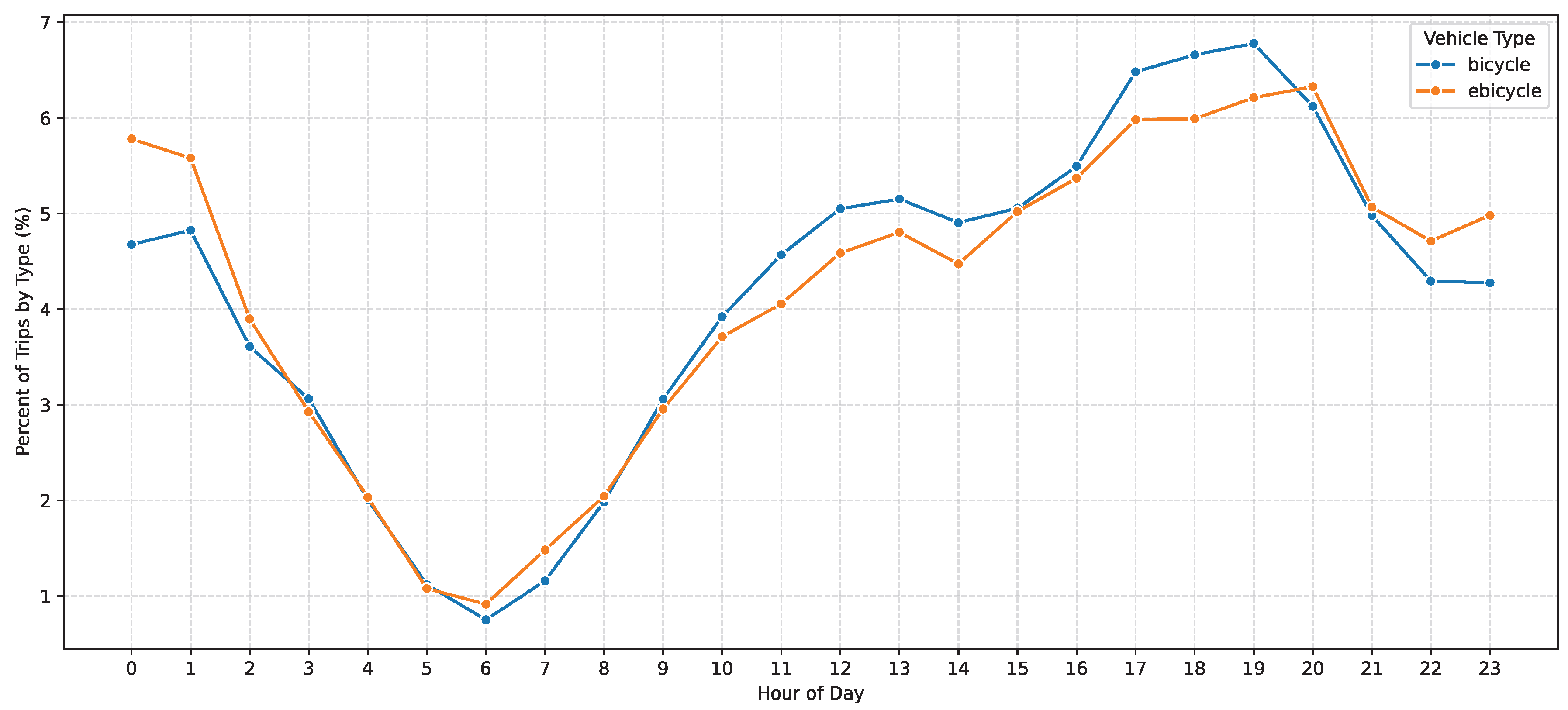
Table 1.
Trip filtering results
| Case Study | Filtering Parameter | Retaining Range | Valid Trips |
|---|---|---|---|
| Bologna | Trip Length [m] | 400<x | 83.7% |
| Trip Duration [s] | 180<x | 88.9% | |
| x<2500 | 98.0% | ||
| Av. Trip Speed [m/s] | 1.00<x | 87.6% | |
| x<6.94 | 97.6% | ||
| Total Retained | 1,389,982 (77.3%) | ||
| Florence | Trip Length [m] | 400<x | 91.6% |
| Trip Duration [s] | 180<x | 93.5% | |
| x<2500 | 98.4% | ||
| Av. Trip Speed [m/s] | 1.00<x | 92.2% | |
| x<6.94 | 93.8% | ||
| Total Retained | 1,822,055 (81.2%) |
Table 2.
Average speed distribution comparison for trip reconstruction validation
| Study | Av. Speed [m/s] | Standard Deviation [m/s] |
|---|---|---|
| This Study | 3.44 | 0.80 |
| ECC 2016 [43] | 4.20 | 1.09 |
| Ratio | 82% | 73% |
Table 4.
Overview of trip parameters distributions (post-filtering) for all modes in Florence.
| Trip Parameter | Percentile & Average | E-bike | Bike | E-Scooter |
|---|---|---|---|---|
| Trip Length [m] * | 10th Percentile | 1028 | 944 | 916 |
| 50th Percentile | 2281 | 2049 | 1825 | |
| 90th Percentile | 4092 | 3979 | 3407 | |
| Mean | 2399 | 2325 | 2023 | |
| Average Speed [m/s] * | 10th Percentile | 2.61 | 2.14 | 1.99 |
| 50th Percentile | 4.41 | 3.36 | 3.82 | |
| 90th Percentile | 6.00 | 4.88 | 5.56 | |
| Mean | 4.35 | 3.45 | 3.80 | |
| Trip Duration [s] | 10th Percentile | 240 | 240 | 240 |
| 50th Percentile | 540 | 600 | 480 | |
| 90th Percentile | 1020 | 1320 | 1080 | |
| Mean | 588 | 717 | 594 |
* Estimated values, see Methodology.
Table 5.
Weekend versus weekday means comparison of trip length, average speed, and trip duration for all modes in Florence.
Table 5.
Weekend versus weekday means comparison of trip length, average speed, and trip duration for all modes in Florence.
| Trip Parameter (Mean) | Transport Mode | Weekdays | Weekends | Variation Weekend/Weekday |
|---|---|---|---|---|
| Trip Length [m] * | E-bike | 2385 | 2440 | +2.3% |
| Bike | 2282 | 2290 | +0.4% | |
| E-Scooter | 2018 | 2036 | +0.9% | |
| Average Speed [m/s] * | E-bike | 4.36 | 4.29 | -1.6% |
| Bike | 3.47 | 3.38 | -2.6% | |
| E-Scooter | 3.84 | 3.71 | -3.4% | |
| Trip Duration [s] | E-bike | 580 | 610 | +5.2% |
| Bike | 710 | 739 | +4.1% | |
| E-Scooter | 585 | 615 | +5.1% |
* Estimated values, see Methodology.
Table 6.
Overview of trip parameters distributions (post-filtering) for all modes in Bologna.
| Trip Parameter | Percentile & Average | E-bike | Bike |
|---|---|---|---|
| Trip Length [m] * | 10th Percentile | 1032 | 838 |
| 50th Percentile | 2082 | 1728 | |
| 90th Percentile | 3772 | 3195 | |
| Mean | 2271 | 1905 | |
| Average Speed [m/s] * | 10th Percentile | 2.08 | 1.83 |
| 50th Percentile | 3.52 | 2.84 | |
| 90th Percentile | 4.95 | 4.00 | |
| Mean | 3.53 | 2.90 | |
| Trip Duration [s] | 10th Percentile | 308 | 288 |
| 50th Percentile | 607 | 613 | |
| 90th Percentile | 1161 | 1243 | |
| Mean | 684 | 704 |
* Estimated values, see Methodology.
Table 7.
Weekend versus weekday means comparison of trip length, average speed, and trip duration for all modes in Bologna.
Table 7.
Weekend versus weekday means comparison of trip length, average speed, and trip duration for all modes in Bologna.
| Trip Parameter (Mean) | Transport Mode | Weekdays | Weekends | Variation Weekend/Weekday |
|---|---|---|---|---|
| Trip Length [m] * | E-bike | 2264 | 2287 | +1.01% |
| Bike | 1905 | 1906 | +0.01% | |
| Average Speed [m/s] * | E-bike | 3.56 | 3.46 | -2.81% |
| Bike | 2.92 | 2.82 | -3.42% | |
| Trip Duration [s] | E-bike | 673 | 709 | +5.35% |
| Bike | 694 | 728 | +4.90% |
* Estimated values, see Methodology.
Table 8.
Comparison of trip parameters between Florence and Bologna case studies.
| Trip Parameter (Mean) | Case Study | E-bike | Bike | E-Scooter |
|---|---|---|---|---|
| Trip Length [m] * | Florence | 2399 | 2284 | 2024 |
| Bologna | 2271 | 1905 | n/a | |
| Florence/Bologna | +5.6% | +19.9% | ||
| Average Speed [m/s] * | Florence | 4.35 | 3.45 | 3.80 |
| Bologna | 3.53 | 2.90 | n/a | |
| Florence/Bologna | +23.2% | +19.0% | ||
| Trip Duration [s] | Florence | 588 | 717 | 594 |
| Bologna | 684 | 704 | n/a | |
| Florence/Bologna | -14.0% | +1.8% |
* Estimated values, see Data and Methodology.
Table 9.
Comparison of median values of trip length, speed, and duration with other case studies.
| Trip Parameter (Median) | Case Study | E-bike | Bike | E-Scooter |
|---|---|---|---|---|
| Trip Length [m] | Florence | 2181 | 2050 | 1825 |
| Bologna | 2082 | 1728 | ||
| 267 European BSS [49] | 1950 | 1750 | ||
| 30 Eur. E-Scooter Sharing [50] | 910-1790 | |||
| Average Speed [m/s] | Florence | 4.41 | 3.36 | 3.82 |
| Bologna | 3.52 | 2.84 | ||
| 267 European BSS [49] | 2.22 | 2.08 | ||
| 30 Eur. E-Scooter Sharing [50] | ||||
| Trip Duration [s] | Florence | 540 | 600 | 480 |
| Bologna | 607 | 613 | ||
| 267 European BSS [49] | 750 | 750 | ||
| 30 Eur. E-Scooter Sharing [50] | 340-826 |
Disclaimer/Publisher’s Note: The statements, opinions and data contained in all publications are solely those of the individual author(s) and contributor(s) and not of MDPI and/or the editor(s). MDPI and/or the editor(s) disclaim responsibility for any injury to people or property resulting from any ideas, methods, instructions or products referred to in the content. |
© 2025 by the authors. Licensee MDPI, Basel, Switzerland. This article is an open access article distributed under the terms and conditions of the Creative Commons Attribution (CC BY) license (http://creativecommons.org/licenses/by/4.0/).
Copyright: This open access article is published under a Creative Commons CC BY 4.0 license, which permit the free download, distribution, and reuse, provided that the author and preprint are cited in any reuse.


