Submitted:
21 November 2025
Posted:
24 November 2025
You are already at the latest version
Abstract
Emerging services such as artificial intelligence (AI), 5G, the Internet of Things (IoT), cloud data services and teleworking are growing exponentially, pushing bandwidth needs to the limit. Space Division Multiplexing (SDM) in the spatial domain, along with Ultra-Wide Band (UWB) transmission in the spectrum domain, represent two degrees of freedom that will play a crucial role in the evolution of backbone optical networks. SDM and UWB technologies necessitate the replacement of conventional Wave-length-Selective-Switch (WSS)-based architectures with innovative optical switching elements capable of handling both higher port counts and flexible switching across various granularities. In this work, we introduce a novel Photonic Integrated Circuit (PIC)-based switching element called flex-Waveband Selective Switch (WBSS), designed to provide flexible band switching across the UWB spectrum (~21 THz). The proposed flex-WBSS supports a hierarchical three-layered Multi-Granular Optical Node (MG-ON) architecture incorporating optical switching across various granularities ranging from entire fibers, flexibly defined bands down to individual wavelengths. To evaluate its performance, we develop a custom network simulator, enabling a thorough performance analysis on all node’s critical performance metrics. Simulations are conducted over an existing network topology evaluating three traffic-oriented switching policies: Full Fiber Switching (FFS), Waveband Switching (WBS), and Wavelength Switching (WS). Simu-lation results reveal high Optical to Signal Ratio (OSNR) and low Bit Error Rate (BER) values, particularly under the FFS policy. In contrast, the integration of the WBS policy bridges the gap between existing WSS- and future FFS-based architectures, manages to relax bandwidth demands and mitigates capacity bottlenecks enabling rapid scalable network upgrades in existing infrastructures. Additionally, we propose a probabilistic framework to evaluate the node’s bandwidth utilization and scaling behavior, exploring tradeoffs among scalability, components’ number and complexity. The proposed framework can be easily adapted for the design of future transport optical networks. Finally, we perform a SWaP-C (Size, Weight, Power and Cost) analysis to underscore the advantages of the proposed architecture. Our results confirm that the proposed node incorporating PIC-based flex-WBSSs, prove to be a cost- and power-efficient solution compared to its counterparts, as reduce excessive initial network deployment/upgrade costs while at the same time minimizing power resource requirements.
Keywords:
Space Division Multiplexing (SDM)
; Ultra-Wide Band (UWB)
; Waveband Selective Switches (WBSSs)
; Photonic Integrated Circuits (PICs)
; full fiber switching (FFS)
; Multi-Granular Optical Node (MG-ON)
1. Introduction
The forthcoming capacity scaling [1,2] driven by bandwidth-demanding services (such as AI, 5G, IoT, cloud data services and teleworking) will further stress optical transport networks. Space Division Multiplexing (SDM)-based optical links and Ultra-Wide Band (UWB) transmission (e.g., over S+C+L bands) constitute a combination that will provide the desirable extra capacity scaling. Consequently, the SDM technology, already commercially deployed in submarine systems [3], is increasingly recognized as a cornerstone for future evolution of backbone networks. In contrast, existing optical node architectures that incorporate WSSs into Reconfigurable Optical Add-Drop Multiplexer (ROADM) nodes to support the UWB transmission may result in very high port counts [4], substantial costs, large volumes of packaging and high installation complexity. Recent research shows that stacked-WDM technology is costly and inefficient at scale, whereas fiber cross-connects can deliver higher throughput and lower blocking probability, reinforcing the need for multi-granular, cost-efficient designs [5]. Consequently, new switching elements should be investigated not only to support UWB switching but also to mitigate the challenge of excessive port counts. In this regard, a recently demonstrated C+L dual-band WSS, capable of grooming 240 wavelengths and enabling more than 3 Pb/s optical-layer throughput ([6]), underscores the rapid industry progress in multi-band switching. Moreover, in emerging Spatial Channel Networks SCNs [7,8], the implementation of hierarchical node architectures seems to be the only feasible solution for effectively supporting the UWB transmission. Accordingly, next-generation optical nodes must be multi-granular, cost-effective, utilizing logical port counts being easily reconfigured, functioning as all-in-one nodes. Several optical node architectures have been proposed ([8,9,10,11]) incorporating these characteristics. All of them feature a two- or three-layer layout and use Optical Cross Connect (OXC) devices to efficiently switch all means of traffic carriers including fibers, bands and wavelengths. A recent study in [12] presents a multi-granular OXC-based architecture utilizing space and wavelength-granular hybrid switching across C- and L-bands, achieving a net throughput of 4.17 Pb/s with a port count of 128. Alternatively, another multi-granular design implementing a double-decker ROADM node supporting UWB switching and incorporating a band cross-connect along with the typical wavelength cross-connect was proposed in [13]. Complementary to these architectural advances, authors in [14] introduced dynamic routing, waveband, and spectrum assignment (RWBSA) algorithms for Multi-Granular Optical Node (MG-ON) networks, offering performance validation and optimization insights that align with the hierarchical architectures. Significant efforts by research consortia are focused on minimizing the chip footprint of existing and future switching elements. Therefore, as advancements in electro-optics and new fabrication techniques are evolving, innovative network elements such as PIC-based WSS and -WBSS are becoming a reality [15]. In this context, recent demonstrations of silicon-photonics-based Mini-ROADMs [16] for packet-optical transport in future 6G-ready networks highlight the feasibility and cost-efficiency of PIC-based reconfigurable nodes.
The introduction of PIC technology offers a cost-effective solution for implementing large port-count WSSs with a small footprint and, as such, they represent a viable alternative for the near future. A design building upon this concept, incorporating PIC-based multi-band WSSs across (S+C+L Bands) was proposed in [17]. This architecture implements S/C/L band-separating Bragg filters coupled with channel-resolving micro-ring resonator filters. The latter is followed by a Mach-Zehnder Interferometer (MZI) switching tree architecture. However, further investigation is required to assess the scalability, volume requirements, and inter-node connectivity of this design. Another node architecture facilitating the transition from multi-band to multi-rail core networks and from wavelength to band/fiber switching was introduced in [18]. This architecture employs fixed band separation filters, ensuring robustness but with limited flexibility and increasing hardware complexity. Authors in [19] proposed a high-port count ROADM architecture that integrates two types of network elements: space and wavelength-routing switches that allow for a cost-effective expansion of the ROADM port count while maintaining acceptable routing performance. In contrast, conventional WSS-based ROADMs [2] require higher port-count switches to accommodate larger node degrees and SDM input fibers, leading to increased size, complexity, and overall cost. This issue can be addressed by hierarchical architectures [4,7,8,20] and WBSSs [9], particularly as multiband transmission emerges as a promising solution [8,13,18]. Previous generation WBSSs utilized concatenating cyclic Waveguide Grating Routers (WGR) along with optical switches [21,22], a combination, however, best suitable for constant bandwidth demands. Furthermore, they operate exclusively within the C-band, not covering the UWB spectrum (e.g. S+C+L -bands). So, what optical nodes urgently need is a flex WBSS. By the term “flex”, we mean the ability to split (if needed) the whole transmission spectrum into flexibly defined contiguous bands and then switch/route each filtered band (or a portion of it) to a specific node’s output port. The proposed MG-ON node, shown in Figure 1, incorporates the novel flex-WBSSs. Leveraging these switches, MG-ON can manage (e.g. divide on demand) and switch everything, from a whole fiber up to a single wavelength channel. The MG-ON was initially introduced in [23] and further analyzed in [24,25].
The main novelty of this work is three-fold: First, we develop a multi-layer, multi-band optical network simulator which models both linear and nonlinear effects in switching layers of MG-ON. The simulator evaluates several traffic policies (FFS, WBS, WS) enabling an extensive performance analysis on all key node metrics, including IL, BER and OSNR.
Second, we explore tradeoffs among scalability, component number and complexity. To support this analysis, we introduce a probabilistic framework for assessing bandwidth utilization and scaling behavior, which can be easily adapted for the design of future optical network deployments or upgrades.
Finally, we perform a detailed SWaP-C analysis, demonstrating the efficiency of our node architecture, followed by a comparison with alternative architectures to highlight its compact design, enhanced energy and superior cost-effectiveness.
The structure of this paper is organized as follows: Section 2 introduces the three-layered architecture of the MG-ON node and provides a thorough analysis of the internal structures of the novel flex-waveband selective switch, and the proposed crossbar switch respectively. Section 3 analyzes all node’s critical performance metrics as a function of traffic loads and network configurations for three different switching policies. Section 4 explores the tradeoffs among scalability, components’ number and node complexity, followed by an evaluation of the optical node's capacity using our proposed probabilistic framework. Section 5 derives cost estimates for the proposed architecture and compares them with alternative switching solutions. Section 6 presents the power consumption analysis of the node. Finally, Section 7 concludes the paper with a summary of our study’s key findings, limitations and outlines future research directions.
2. MG-ON Three-Layered Architecture
The three-layered MG-ON hierarchical architecture is illustrated in Figure 1. The flex-WBSSs are located at the highest hierarchy, Layer 1—(Flex-Band Route and Select) of MG-ON. All incoming (and outcoming) fibers are connected “hard-wired” to the ingress and egress WBSSs modules, in a Route-and-Select (R&S) mode. Layer 1 is responsible for switching either the filtered disjoint bands or the full fiber content (in express traffic mode) of traffic passing through the node (L1P and L1PE in Figure 1 respectively). In the case of FFS, the Finite-Impulse Response (FIR) filters are set to pass-through mode, thus bypassing all the filtering delays of WBSS (FFS inset in Figure 1). A 3-degree node is illustrated in Figure 1, with the possible light-paths from West to East or South denoted as solid black lines. SDM spatial dimensions for East and West are equal to three, while South are equal to two respectively. Finally, Layer 1 can support Spatial Lane Change (SLC) providing the relocation of bands from one input spatial lane to another in case of a link failure, at the cost of higher port count WBSSs due to additional output ports needed. The intermediate hierarchy, Layer 2—(Flex Band Add/Drop) is responsible for Flex Add/Drop bands from/to local premises or other smaller sub-networks.
Figure 1.
Hierarchical (3-Layered) Multi-Granular UWB/SDM Optical Node (MG-ON) architecture. Insets: FFS, WBSS.
Figure 1.
Hierarchical (3-Layered) Multi-Granular UWB/SDM Optical Node (MG-ON) architecture. Insets: FFS, WBSS.
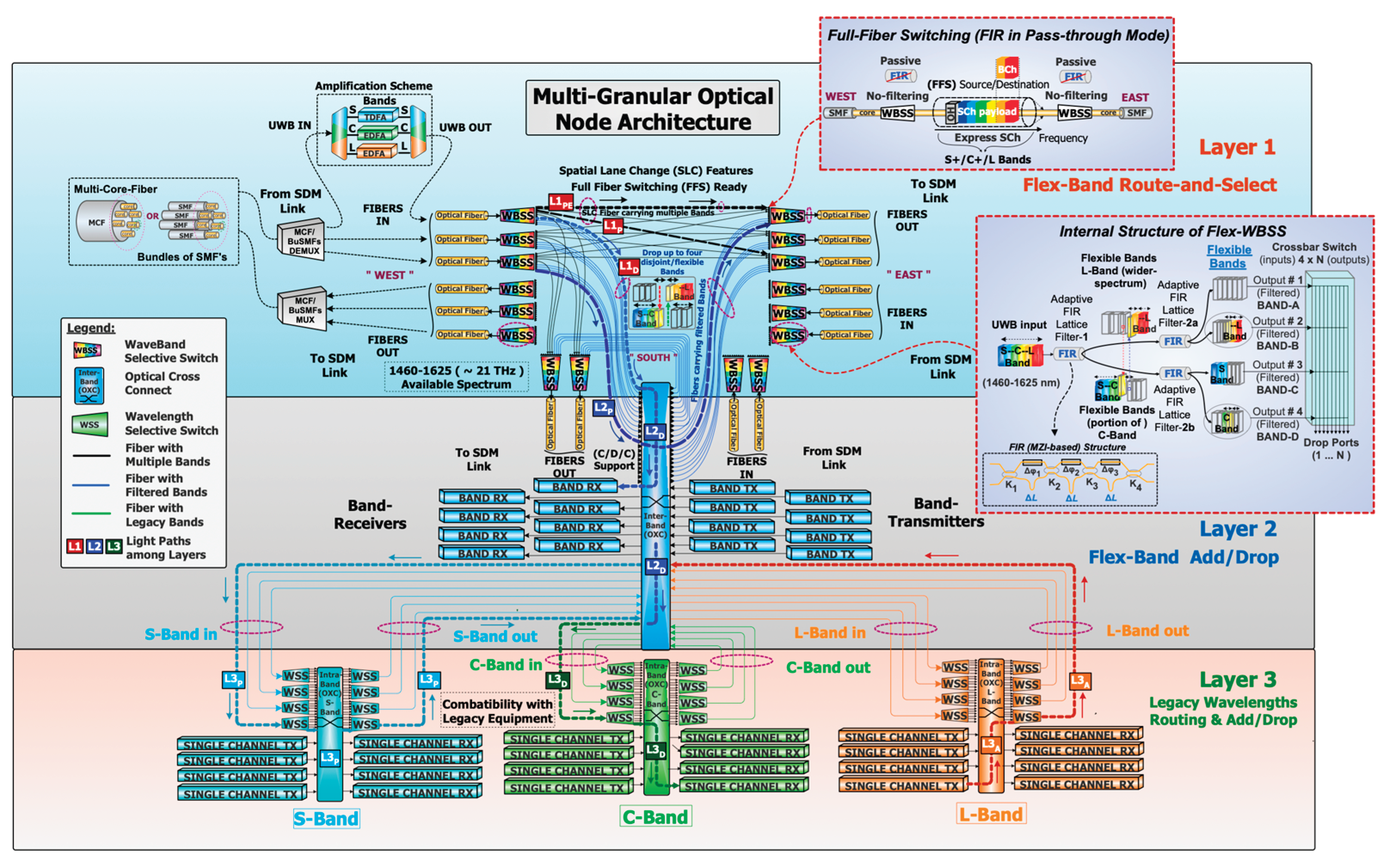
Layer 2 relies solely on an Inter-Band Optical Cross Connect (OXC) which can manage and receive/forward bands (or portion of bands) in a Colorless/Directionless/Contentionless manner (C/D/C) [24] from/to the local band-transceivers. Blue lines from the West ingress WBSS direct the selected flex-bands to the OXC (L1D in Figure 1) which can either assign each dropped band to an available band receiver (L2D in Figure 1) or passes through the selected flex-bands to another degree (L2P in Figure 1), either to improve the traffic management or/and to provide enhanced redundancy and resilience. Similarly, the blue lines from the OXC to the East/South egress WBSS represent additional paths for signals originating from band-transmitters, with the reconfiguration association performed by the OXC. For clarity, other blue connection lines are omitted. Finally, the lowest hierarchy, Layer 3—(Legacy Wavelengths Access for Routing and Add/Drop) ensures compatibility with legacy equipment such as C-band transmission systems. Bands S, C and L, which require wavelength access, are configured via conventional WSS interfacing with an Intra-Band OXC. This setup supports routing and/or wavelength add (L3A in Figure 1) or drop (L3D in Figure 1) to single-channel transceivers. The choice for passing individual wavelengths through the node to another degree is another option too (L3P in Figure 1). As wavelength access is expected to be phased out gradually, resources at this layer can be decommissioned over time and replaced by scalable elements of Layer-2 (e.g. WBSSs, band-transceivers).
2.1. Internal Structure of WBSS
The novel MG-ON architecture aims to address the transition from current wavelength switching to future full fiber switching through an intermediate step to waveband switching, being compatible with all these technologies. It incorporates PIC-based, state-of-the-art flex-WBSSs comprising features such as reduced size footprint, low insertion losses (few dB), fast switching (found to be in the range of 10 microseconds when utilizing piezo actuators on silicon nitride waveguides) combined with a low-cost signature. The expected crosstalk suppression is roughly ≥ 23 dB at the output. The internal WBSS structure depicted in Figure 2(a) incorporates two adaptive filtering stages implemented with cascaded optical FIR lattice filters (Figure 2(a), inset) [22,23], where k₁–k₄ represent the coupling coefficients, Δφ₁–Δφ₃ the tunable phase shifters, and ΔL segments indicate the optical path length differences between the two arms of each MZI stage. These filters can split the incoming traffic into one up to four flexible disjoint bands. After this stage, the bands are routed to a 4×N non-blocking Crossbar Switch (CS) which directs each band (or portion of it) to a designated output port.
Figure 2(a) shows the internal structure of flex-WBSS and its filtering operation. Figure 2(b) shows a fabricated compact prototype of the WBSS/crossbar-switch PICs on a large silicon nitride wafer. Figure 2(c) depicts the packaged module of a WBSS/switch PIC designed for seamless integration in the MG-ON node. The UWB switching scenario is illustrated in Figure 2(a) where the incoming UWB signal (S+C+L bands) is divided into three disjoint parts and routed to three different outputs out of four possible ports.
In the 1st stage (Filter-1) of adaptive FIR lattice filtering, the spectrum of the UWB signal is divided into two segments: the first segment includes the L-band and a portion of the C-band (forwarded to the top stream), and the second segment includes the S-band and the remaining C-band (forwarded to the bottom stream).
The 2nd stage of adaptive FIR lattice filtering comprises two main cases. In the first case if no further splitting is required on the top stream, the Filter 2a is set to pass-through mode (no filtering performed Figure 1 inset) and so the top stream remains unchanged. (Denote that the MZI lattice elements can be configured in two modes. The first is the pass-through mode: traffic traverses only one arm of each MZI and so is not filtered at all, so it emulates the WBSS to a simple fiber switch. The second mode performs band filtering as designed).
Afterwards in the second case, the Filter 2b splits the bottom stream into two parts: one containing the S-band and the other containing a portion of the C-band. So, in this switching scenario the resulting carved bands are:
The CS relies on a non-blocking layout ensuring that each of the four bands (or any segment/combination of them) can be independently directed to one of its output ports. The total number of filter taps used defines the sharpness of the lattice filters. If we need a finer resolution, we must use more taps. In such a case, the optical delay is affected by the larger bandwidth that the filter can support (spanning 165 nm ~ 21 THz total bandwidth). Our filter design is based on a low-pass filter. In this filter we must specify the pass-bandwidth, the block-bandwidth, the attenuation specification (-23 dB) and the number of filter taps. The transition band (the gap between the passband and the block-band) is the bandwidth used at the transition time when the filter drops from the pass to the block band. Of course, a narrow transition band would be more desirable as it would ensure a sharp transition. So, we control the transition sharpness by altering the number of filter taps: more filter taps ensure a sharper filter transition as in the following Figure 3.
Our simulation results of transmissivity versus frequency for four flexible disjoint bands, using 20 and 40 taps, are shown in Figure 3(a) and Figure 3(b) respectively, and validate the aforementioned values. Should we choose to increase the number of taps (e.g., by a factor of 2) this results in a broader, continuously flat-top band shape, a narrower transition bandwidth (from 2.318 to 1.098 THz) and sharper filtering transitions.
The number of taps is given by:
2.2. The Innovative Design of the Crossbar Switch (CS)
The proposed crossbar switch utilizes tunable couplers, which are implemented as single-stage MZIs with equal arm lengths. One arm of the MZI incorporates a phase actuator, enabling the formation of a coupler with a variable coupling ratio. When the input light enters the MZI, it is split into two arms. By adjusting the phase in one of the arms, the interference upon recombination at the output can be controlled to be either constructive or destructive. This phase-tuning capability allows the input signal to exit the MZI through either the bar port, cross port, or a combination of both, contingent upon the specific phase adjustment applied. The internal structures of (4-input/N-output) CS for two different implementations are depicted in Figure 4. The conventional implementation features an array of inputs connected to an array of outputs, typically arranged in rows and columns (see Figure 4(a)). At each intersection of these waveguides, an MZI is positioned. To create an association between each input and output, the intersecting MZI is adjusted to redirect the input signal, which travels through the horizontal waveguide, to the designated output on a vertical waveguide. In this configuration, most switches are set to the cross-state, while the switch that establishes the connection is set to the bar-state (see Figure 4(a)). In our proposed CS’ design (in Figure 4(b)) we invert the logic at each intersection. This approach requires the most MZIs set to the bar state and complements the operation with a waveguide crossing. When a traffic flow enters the CS from input port 1, it can be seamlessly switched to any one of the N=6 output ports just by configuring the adjacent tunable couplers (which are set to either bar or cross-state). So, the signal in the CS may pass through one crossing where the MZI drops the signal, which is set to bar state (minimum, best-case scenario) up to 3+N crossings (maximum, worst-case scenario). Crosstalk optimization, in our proposed architecture, requires pre-setting all tunable couplers to the bar-state, except at the one selecting the desired output (drops the signal which set to cross-state) port. This configuration leverages waveguide crossings, as shown in (Figure 4(b)) while the conventional one is missing them (Figure 4(a)). Nevertheless, this approach may incur additional waveguide losses. In the following section, we present simulation studies for both implementations which determine the approach with the optimal performance.
3. Performance Evaluation of MG-ON Node
In theory the WBSS operates with negligible losses. However, in practice, the WBSS Insertion Loss (IL) depends on: the number of FIR filter’s taps (~0.1 dB/tap) that are used, the accuracy that the directional couplers (DCs) across S+C+L bands can achieve, and finally how many times the signal passes through the crossbar crossings in the CS (~0.05 dB/junction), (Figure 1, inset).
3.1. Performance Evaluation of WBSS Components
The signal in the CS may pass through from one crossing up to 3+N crossings and varies with specific wavelength. The average IL is calculated upon all cases (from best to worst), for all (four bands) and then divided by eight (two paths for each band). Optimal performance of both components (FIR and CS) necessitates precise 50:50 power splits, which can be achieved using stabilized DCs (Figure 5(a)). The IL of lattice filters, as noted earlier, is a function of the number of taps used. This number is an a priori parameter normally set by the node designer. Typically, the CS’s switches are set to the cross-state (except for the selected intersection switch which is set to bar-state). However, conducted studies in [24] revealed that the bar state has a slightly better performance than that of the cross-state. So, it is preferable to invert the state of CS’s switches and finally set most MZIs at the bar state and use a waveguide crossing to at each intersection (see Figure 4(b)) to achieve an improved CS performance. So, if a waveguide crossing shows better performance than a DC, then this method turns out to be beneficial. Waveguide crossings in general do not create significant crosstalk, but they result in low values of IL. As a result, this method introduces a trade-off between crosstalk and IL. In any case, we must take into consideration that crosstalk is the most critical performance metric. Figure 5(a) depicts the performance of a coupler with stabilized DCs (50:50); Figure 5(b) shows the simulated output of a single lattice stage (unitary transformation with tunable coupler, MZI delay, tunable coupler), set to 50:50 power splits and varying the delay phase to scan the notch frequency. Figure 5(c) shows the performance of a 4×19 CS for two separate designs: direct (MZIs in bar-state) and traversed (MZIs in cross-state).
The IL is derived by the equation:
3.2. Simulation Results Using the Developed Multi-Layer Optical Network Simulator Implementing Three Different Traffic-Oriented Policies
We have built a multi-layer, multi-band optical network simulator designed to evaluate node’s key transmission performance metrics such as OSNR and BER. Several diverse impairment scenarios, attenuation profiles, and traffic loads across various network layers of the node are examined. The simulator provides a Quality of Transmission (QoT) estimation along with signal penalties analysis by thoroughly modeling both linear and nonlinear physical layer impairments across the S-, C-, and L-bands. It also incorporates a wide range of modulation formats—Quadrature Phase Shift Keying (QPSK), 8-Quadrature Amplitude Modulation (QAM), 16-QAM, and 64-QAM—as well as multiple switching paradigms, enabling robust performance assessment and network optimization. The simulation framework evaluates three basic traffic switching policies/scenarios: Full Fiber Switching (FFS), Waveband Switching (WBS), and Wavelength Switching (WS), each mapped to different MG-ON layers (Layers 1, 2, and 3, respectively). These scenarios allow comparative analysis under varying traffic distribution and allocation schemes (e.g., L1, L2 and L3 cases shown in Figure 1). Other simulation parameters include amplifier specifications [26], such as Thulium-Doped Fiber Amplifiers (TDFAs) for the S-band and Erbium-Doped Fiber Amplifiers (EDFAs) for the C- and L-bands respectively. Nonlinear impairments—including Four-Wave Mixing (FWM), Stimulated Raman Scattering (SRS), Raman tilt—as well as linear effects such as Polarization Mode Dispersion (PMD), are also incorporated into the simulation. Finally, the simulator also models IL across key MG-ON’s optical elements, including WBSSs, FIR filters, Crossbar Switches (CSs), Inter/Intra Optical Cross-Connects (OXCs) and WSSs.
Figure 6 illustrates the OSNR and the corresponding traffic load—ranging up to 10 Pb/s—across various switching scenarios and flexible transmission bands (S-, C-, and L-bands) of the MG-ON.
Simulation results indicate that the OSNR degrades with increasing traffic load. This degradation is driven by both nonlinear effects (e.g., SRS, Raman tilt, FWM) and linear effects (e.g., PMD and insertion losses derived from MG-ON components such as WBSSs, FIRs, CSs, and OXCs). Scenario-based curves emphasize the impact of varying loss profiles (L1–L3 light paths shown in Figure 1) and traffic allocations for Full Fiber Switching (FFS, Scenario 1), Waveband Switching (WBS, Scenario 2), and Wavelength Switching (WSS, Scenario 3) policies across flexible S, C, and L bands. Our simulation results reveal that the S-band exhibits the steepest degradation, followed by the L-band, while the C-band performs best. Scenario 1 (FFS) maintains the highest OSNR due to minimal losses, as FIRs are in passthrough mode (depicted in Figure 1 inset) and no OXCs are utilized. Scenario 2 (WBS) shows moderate performance (missing gap on existing architectures), while Scenario 3 (WS) experiences the lowest OSNR due to cumulative insertion losses (note that WS is only used for legacy support). At higher traffic loads, the degradation in OSNR becomes significantly more pronounced (as expected), highlighting the impact of nonlinear effects, optical losses, and traffic loads.
The BER (on a logarithmic scale) shows increasing error rates as traffic load rises, driven by OSNR degradation due to linear and nonlinear effects discussed above. Scenario-based curves highlight the influence of loss profiles and traffic allocation schemes on BER across S, C, and L bands under three switching policies: Full Fiber Switching (FFS, Scenario 1), Waveband Switching (WBS, Scenario 2), and Wavelength Switching (WSS, Scenario 3). As shown in Figure 7, the BER increases with higher traffic loads due to cumulative impairments. Comparing individual bands’ performance, the S-band has the highest BER, the L-band achieves moderate values, and the C-band achieves the lowest BER among all bands. Comparing different switching scenarios’ performance, Scenario 1 (FFS) has the lowest BER (ranging from 10E-9 to 10E-2), while Scenario 2 (WBS) achieves moderate BER values (ranging from 10E-5 to 10E-2). Finally, Scenario 3 (WSS) has the highest BER (10E-2 to 10E-1) due to greater losses. At higher loads (e.g., 9–10 Pb/s), differences in BER across bands and scenarios become less pronounced.
4. Scalability Challenges of MG-ON
In this section we analytically derive the number of MG-ON’s devices as they affect not only the performance metrics but also the deployment cost of the proposed node. Another critical factor that directly affects both performance and the efficiency is the number of spatial lanes and the node’s degree of connectivity. Accordingly, we explore the trade-offs between scalability, component count and complexity, along with the corresponding throughput, for various configurations in the three-layered MG-ON architecture.
4.1. Proposed Model and Assumptions for Scalability and Throughput Analysis
Table 1 lists the key design parameters along with their description and usage which are used in order to explore the scalability and achievable throughput performance of the MG-ON architecture.
- ▪
- Regarding the computations of the total count of band-transceivers, we consider the individual units of transmitters (Tx) and receivers (Rx).
- ▪
- Regarding total throughput, we consider only the incoming traffic from wherever is entering the node.
- ▪
- Regarding the computations of the total traffic (and thus throughput) entering from the band-transceivers located at Layer 2, we use a bandwidth of ~0.5 THz for all guard bands used to account for the transition bandwidth lost in the entire UWB spectrum.
So, for the whole UWB spectrum, the defined guard bandwidth (), the total number of guard bands (, and for a specific spectral efficiency (SE), the total MG-ON throughput is derived by:
For MG-ON’s Layer-1: The WBSSs needed for R&S, for degree (D) and spatial lanes (Si) is given by:
The total port count of all deployed WBSS’s for degree (D) considering SLC capability is given by:
If we do not consider the ability of SLC we result in a lower number of ports, given by:
By KB we denote the number of ports (in each WBSS) that are allowed to serve split bands destined for add/drop. As the total number of bands is 4, KB takes values from 1 to 4. So, when SLC is enabled, any incoming band can be routed to any WBSS in any direction across all degrees.
For MG-ON’s Layer-2: The number of ports of the Inter-OXC located at Layer-2 is given by:
Note that NBTx /NBRx is the total number of band transmitters/receivers (located at the MG-ONs add/drop section in Layer-2) and KW is the Inter-OXC’s total number of ports dedicated to wavelength granularity of Layer 3.
Suppose that G denotes the percentage of granularity used (e.g. G=2 with 50% granularity and G=4 with 25% granularity), then eq. (8) gives us the total number of band-transceivers for different values of G.
4.2. Proposed Probabilistic Framework for Band Modelling of MG-ON
The MG-ON is characterized by the degree of connectivity (D) to neighboring nodes and the number of spatial lanes (S) per link. Traffic on a link is distributed across the S spatial lanes (fibers), but the question arises on the number of flexibly defined bands we can expect to have on each fiber. Efficient traffic routing attempts to pack flows to existing bands across the S fibers that are destined for the same network site. An efficient network design would attempt to pack traffic into a minimal number of fibers, which would lead to four bands per fiber and lost BW due to transitions. Since the future belongs to FFS (no separate band handling), a common ground we develop herein strikes a balance between bands and fibers.
An assumption we make is that for low spatial (parallelism) lanes (e.g., S=3), fibers will tend to have more bands. In our node design, we set the max number of bands equal to 4. Overall band count (and destination grouping) is capped at 12. At high spatial (parallelism) lanes (e.g. S=12), fibers will tend to have fewer bands (skewed towards 1 and 2 bands, rather than 3 or 4). At minimum we have 12 full fiber bands, and higher when 2 bands (or higher) are utilized per fiber.
To model the expected bands per fiber, we adopt the binomial distribution model below. The probability for value x in a binomial distribution is:
for integers from 0 up to n. Since the distribution starts at 0, we will essentially count the number of guard bands between 0 and 3 (accordingly for band counts from 1 to 4).
Expected Total Bands:
For example, for S=12, using p=0.125:
There’s about a 67% probability that there will be 0 guard bands (1 band total) per fiber.
Binomial Model: The number of bands on each fiber is modeled using the binomial distribution:
where S is the number of trials (Fiber per link)
Total number of Bands for (S) spatial lanes (fibers) among degrees (D) is given by:
where is drawn from the bionomial distribution above.
So, taking into account the above, the distribution can be expressed as:
where:
- Total Bandwidth is the total UWB spectrum across S+C+L bands (~21 THz).
- is the number of guard bands used after FIR filtering.
- is the transition bandwidth lost from the entire UWB spectrum (with each guard band has an approximate bandwidth of ~0.5 THz).
Figure 8 shows how the number of bands expected per fiber can be modeled with the binomial distribution Eq. (9-10) mentioned above. The top x-axis gives the probability of different band counts (e.g., 1–4 bands) from Eq. (10-11), while the bottom x-axis shows the equivalent number of guard bands (defining the unused spectrum due to band-transitions). As the spatial degree (S) increases from 3 fibers Figure 8(a) up to 12 fibers Figure 8(d), the distribution shifts: at low S values, fibers tend to carry more bands while at high S values, fibers are more likely to have fewer bands (1–2) thus reducing the guard-band overhead.
4.3. Simulation Results
After determining the minimum and maximum number of bands using our probabilistic framework for band modeling of MG-ON (for each value of S), we next evaluate how MG-ON scales across different implementations—small, medium, and large number of degrees (D=3, 4, 5) with respect to the proposed values of spatial lanes S and the corresponding number of bands. Furthermore, we compute the total throughput (minimum and maximum values) depending on the transition-loss bandwidth associated with the number of bands.
Figure 9 evaluates the scalability of WBSS components in MG-ON Layer-1 with necessitate ports (KB) embedded for add/drop traffic capabilities.
On the horizontal axis we evaluate spatial lanes (S) ranging from 3 up to 12 for varying degrees of connectivity (D)= 4, 5, 6 simulating a small-, medium-, and large-scale node respectively. The left vertical axis indicates the number of required components while the right vertical axis evaluates the achievable throughput (ingress traffic to MG-ON node). Results show that increasing the number of spatial lanes leads to a rise in both the number of components and the achievable throughput. For example, a small-scale node with S=3 and D=4 needs the deployment of 24 1×11 WBSSs and achieves a throughput of minimum ~2.63 Pb/s to maximum ~2.71 Pb/s. A medium-scale node with S=6 and D=5 requires the deployment of 60 1×26 WBSSs and reaches a throughput of ~6.64 Pb/s up to ~6.75 Pb/s. Finally, a large-scale node with S=12 and D=6 requires 144 1×62 WBSSs and delivers a throughput of roughly ~16.70 Pb/s up to ~16.78 Pb/s. The achievable target of 10 Pb/s or higher is attained with a D equal or greater than 5 at S=9, reaching approximately of ~10.14 Pb/s to ~10.36 Pb/s necessitating the deployment of 90 1×38WBSSs.
Figure 10 illustrates the relationship between spatial lanes and system performance for INTER-OXC located at MG-ON’s Layer-2.
From Figure 10 we indicate that both the port count and the achievable throughput increase with the number of spatial lanes. For example, for a large-scale configuration, at S=12 and D=6, the system delivers a maximum throughput exceeding 6.13 Pb/s and minimum of ~4.77 Pb/s with the deployment of approximately 468 ports. A medium-scale configuration with D=5 and S=6 reaches a maximum throughput of roughly 3.29 Pb/s and minimum around ~2.78 Pb/s using 196 ports. Lower-degree configurations (small-scale nodes) require fewer ports but as expected, deliver lower throughput; for instance, with S = 3 and D = 4, the system achieves about 1.10 up to 1.26 Pb/s with the deployment of 78 ports. We conclude that while increasing the number of spatial lanes directly boosts performance, it does so at the cost of a significantly higher port count.
Figure 11 shows the Layer-2 throughput along with the number of band-transceivers for various numbers of spatial lanes (S).
As expected, the number of band-transceivers scales with the spatial lanes, with higher degrees enabling slightly higher throughput. For example, the highest throughput of 0.93 Pb/s is attained at S=12 utilizing 36 band-transceivers (Tx/Rx). A modest throughput of up to 0.56 Pb/s is attained at S=9 deploying 22 band-transceivers (Tx/Rx). Finally, the lowest throughput of ~0.15 Pb/s achieved at S=3 required 6 band-transceivers (Tx/Rx). However, this configuration is less performance-intensive compared to WBSS or INTER-OXC systems.
5. Technoeconomic Analysis
Techno-economic analysis of any new technology is an essential task towards going commercial. The envisioned flex-WBSS is proposed as a PIC solution, as this approach generally offers a significantly reduced SWaP-C (Size, Weight, Power and Cost) factor compared to other possible implementations (such as wideband WSSs utilizing free space optics).
5.1. MG-ON’s Cost Model
The MG-ON’s cost model considers the total number, the port-count, and the relative cost of its key components.
For each component type i ∈ {WBSS, Inter-OXC, Band-transceivers},
The cost can be expressed as:
While the total MG-ON node cost is given by the following equation:
Where:
- is the baseline relative cost of an element at the reference size (e.g. regarding WBSSs, the reference size 1×9 WBSS with Cost ≈1).
- is the element’s actual number of ports.
- is the element’s reference number of ports (see Table 2).
- is the number of elements of type i with size N (e.g. WBSS, OXC, Band-transceivers).
- is the scaling factor, which specifies the relative increase in cost per quadrupling of ports.
We assume a well-known general rule suggesting that “In practice, a new technology is assumed to displace its predecessor only when it delivers ~4× higher throughput while keeping cost ≤ 2.5× that of the previous generation [27]”. However, in our context, this typically corresponds to a substantial increase in port count per element.
Simulation assumptions: We implement the assumption by setting:
This corresponds to ~4× higher port count while keeping cost ≤ 2.5× the increase in relative cost. The same value α is applied to band-transceivers with the scaling further adjusted proportionally to the number of wavelengths λ to account for multi-λ operation.
Table 2 presents the relative cost (RC) of the MG-ON components, normalized to that of a 1×9 WBSS (which is the base in the cost analysis).
5.2. Cost Analysis of the Key MG-ON Components
Figure 12 illustrating the cost analysis of the MG-ON architecture, derives the relative cost contribution of its key components across Layers 1 and 2 (Figure 1). We evaluate the cost for different configurations with varying numbers of spatial lanes (S=2, 4, 6, 8) and degrees of connectivity (D=3, 4, 5), with (KB=4) full drop bands (used to estimate the full-scale node cost) corresponding to three different node implementations.
In the Figure 12, the x-axis represents the number of spatial lanes per degree (S), ranging from 2 to 8 while the y-axis shows the total relative cost, normalized to the cost of a 1×9 WBSS (see Table 2). Different colors and bar groups correspond to the costs of PIC-based WBSSs, both with and without SLC support, together with supporting components including C- and L-band EDFAs, S-band TDFAs, Inter-OXCs, and band-transceivers. The cost model defined in Eq. 13 is applied to compute the relative cost considering both the type (WBSS, Inter-OXC, Band-transceivers) and the port count of each component. Simulation results reveal that, if we leave out the SLC feature we do achieve substantial cost reductions, making this option particularly suitable for SCN networks highlighting a trade-off between cost savings and redundancy.
For instance, in a large-scale node configuration (D=5, S=8), the deployment cost reaches approximately 207.20 CUs employing 80 1×36 WBSSs in Layer 1 with SLC support. In contrast, without SLC the cost decreases to 80 CUs by employing 80 1×8 WBSSs, corresponding to an improvement of nearly 2.5-fold. For a medium-scale configuration (D=4, S=6) the cost amounts approximately to 99.36 CUs when incorporating 48 1×22 WBSSs with SLC support, whereas without SLC, the cost drops by about 50% to 48 CUs using 48 1×7 WBSSs. Similarly, in small-scale implementations (D=3, S=4) we have to spend 33.60 CUs with SLC utilizing 24 1×12 WBSSs, whereas without SLC, the cost decreases to 24.00 CUs with 24 1×6 WBSSs , representing a 29% cost reduction.
The cost of the Inter-OXC in Layer 2 also scales with node size though at a considerably lower rate than other MG-ON’s components. A large-scale implementation (D=5, S=8) needs only 19.16 CUs deploying an OXC with 364 ports, whereas a medium scale-implementation (D=4, S=6) requires 14.66 CUs deploying an OXC with 220 ports. In contrast, a small -scale node (D=3, S=2) requires only 5.86 CUs with 58 ports.
As expected, the number of band-transceivers scales with the spatial lanes, with higher degrees leading to higher costs compared to other equipment. For a large-node deployment (D=5, S=8), 160 CUs are required incorporating 20 band-transceivers (Tx/Rx). A medium-scale node (D=4, S=8) requires 128 CUs for 16 band-transceivers represent a ≈ 20% cost reduction compared to the previous configuration. Finally, a small-scale node (D=3, S=6) required 72 CUs for 16 band-transceivers, yielding a 55% cost reduction compared to the large configuration.
For amplification schemes, specifically for EDFA and TDFA amplifiers, the cost analysis reveals consistent trends across different node sizes. In large-node deployments (D=5, S=8), the required CUs are 40 and 48 when deploying 80 C- or L-band EDFAs, respectively, whereas 96 CUs are required with 80 TDFAs, resulting in an approximately 2-fold cost increase for TDFA-based implementations. For medium-scale nodes (D=4, S=4), the cost amounts to 16 and 19.2 CUs when deploying 32 C- or L-band EDFAs, respectively, compared to 38.4 CUs with 32 TDFAs, corresponding to a 2-fold higher cost. Similarly, in a small-scale node (D=3, S=2), 6 and 7.2 CUs are required with 12 C- or L-band EDFAs respectively, while 14.4 CUs are needed with 12 TDFAs, confirming a ≈200% higher cost for TDFAs.
5.3. Comparative Analysis of the Proposed Versus Other PIC- and Non-PIC-Based Alternatives
Previous technoeconomic studies that examined the broader potential of multi-band optical networks were presented in [28,29]. Performing a fair cost comparison among different node architectures is inherently challenging, since each solution relies on distinct components and exhibits different performance characteristics. It should be emphasized that this evaluation serves only to highlight the potential advantages of the proposed technology, rather than to provide an absolute cost comparison, as actual deployments involve numerous complex and variable factors. To ensure consistency, we adopted a best-effort benchmarking approach based on normalized costs to a single 1×9 WBSS, thereby allowing all designs to be evaluated under a common reference framework. Using this methodology, we extend our analysis by conducting a cost comparison of the proposed MG-ON architecture against other (PIC- and non-PIC-based) WSS alternatives ([17,18,30]).
Figure 13 presents the cost comparison of MG-ON WBSS-based architecture and alternative WSS-based solutions for various spatial lanes S=(2, 4, 6, 8) and node degrees of connectivity D= (3, 4, 5). The vertical axis shows the total node cost normalized to that of a single 1×9 WBSS, enabling direct comparison across architectures. As shown, the MG-ON design achieves a clear cost advantage across the most evaluated scenarios, with the largest savings occurring when SLC support is not enabled, particularly in cases C(1), C(6), and C(11) (indicated by *).
For small degrees, MG-ON offers significant cost reductions compared to all alternatives. For example, for S=6 and D=3, MG-ON incurs a relative cost of 36 CUs without SLC and of 59.04 CUs with SLC enabled, while the multi-band PIC-based WSS, conventional WSS-only, and hybrid-WSS architectures require 73.44 CUs, 80.84 CUs, and 152.56 CUs, respectively. This corresponds to more than a 5-fold cost reduction compared to the hybrid-WSS solution (with SLC disabled), a 20% up to 50% improvement over multi-band PIC-based WSS, and a 27% up to 55% improvement relative to WSS-only conventional architecture depending on SLC use or not.
The scalability benefits of MG-ON become more apparent at higher degrees especially without SLC support. For example, for S=6 and D=5, MG-ON requires 60 CUs without SLC and 155.40 CUs with SLC. Similarly, the multi-band PIC-based WSS architecture achieves 193.80 CUs, the conventional WSS-only achieves 132.73 CUs, whereas the hybrid-WSS architecture reaches 446,60 CUs, representing a 3.0 up to 7.0× cost advantage. In contrast, the WSS-only architecture slightly outperforms MG-ON only when SLC is enabled, offering about a 17% lower cost, whereas MG-ON remains more economical when SLC is disabled, providing roughly a 54.8% cost advantage.
Similar trends are observed at higher spatial lane counts. For example, at S=8 and D=5, the MG-ON cost is 80 CUs (without SLC), and 207.2 CUs (with SLC), compared to 271.20 CUs for multi-band PIC-WSS, 176.78 CUs for WSS-only, and 594.8 CUs for hybrid-WSS approach. In this configuration MG-ON achieves 23,6 up to 70.5% cost reductions compared to multi-band PIC-WSS and a 2.87- up to 7.43-fold cost reduction compared to hybrid-WSS architecture. Conventional WSS-only architecture can slightly undercut MG-ON by roughly 14.7 percent when SLC is enabled, but MG-ON maintains better scalability overall.
To sum up, among all the alternatives, the hybrid-WSS architecture is consistently the most expensive. Its cost rapidly escalates with both spatial lanes and degrees of connectivity due to the compounded requirements of large-port WSS modules and multiple OCS elements. For instance, at S=8 and D=5, the hybrid-WSS cost reaches 594.8 CUs, the highest across all evaluated scenarios.
The conventional WSS-only design exhibits intermediate behavior. For lower degrees (D=3), it remains more costly than MG-ON, but at higher degrees its costs converge toward or even slightly undercut those of MG-ON. This inversion reflects a trade-off: WSS-only designs avoid the additional interconnect and banding overhead of MG-ON, but they scale poorly with increasing S, making them less attractive in large-scale scenarios. The multi-band PIC-based WSS approach provides moderate improvements over conventional and hybrid designs but remains consistently above MG-ON. Its costs grow from 73.44 CUs at S=6 and D=3, to 271.20 CUs at S=8 and D=5, exceeding MG-ON by 20–40% across the operating range. This overhead arises from the requirement for additional multiplexing/demultiplexing stages, which offsets the benefits of photonic integration. In summary, the results depicted in Figure 13 confirm that MG-ON offers the most favorable cost–scalability trade-off among all the compared architectures. It achieves substantial cost savings compared to hybrid-WSS (up to more than 7.5× at S=8 and D=5), remains consistently more efficient than multi-band PIC-WSS, and competes closely (when SLC support disabled) with conventional WSS-only designs. The trade-off lies in functionality: MG-ON without SLC minimizes cost but sacrifices flexibility, whereas enabling SLC increases the WBSS size and associated cost at the benefit of enhanced redundancy and resilience. Finally, both the proposed MG-ON and the multi-band PIC-WSS architectures exhibit reduced volume of packaging and lower deployment expenditures compared with non-PIC-based solutions, thereby achieving a smaller SWaP-C factor.
6. Power Consumption Evaluation
Industry consortia and collaborative research initiatives are actively exploring ways to reduce energy consumption and, so, end up with energy-efficient designs. One promising approach is the adoption of optical bypass technology in network elements, which minimizes electronic terminations by implementing energy-efficient PIC-based solutions ([23,31]). In the MG-ON design, each WBSS, regardless of its port count is equipped with a control unit driven by an Algorithmic Intelligent Controller (AIC). The AIC implements Control and Calibration (C&C) algorithms, as described in [32], which provides C&C of WBSS PICs [33], thereby enhancing overall energy efficiency.
6.1. Power Consumption Model for the Proposed MG-ON
As the number of required WBSSs scales differently for the examined degrees, the overall power consumption of the node due to the control unit scales accordingly. Based on internal data from our partners, this control unit consumes a fixed power of 1.5 watts for every PIC-based WBSS module [23] and approximately 75 watts for a single 192×192 Inter-Band OXC [23] (see Table 3) in order to operate flawlessly. For band-transceivers, this scaling is further applied proportionally with the number of wavelengths λ (approximately 15 for a band-transceiver), with a baseline of 13.81 watts per single wavelength, to account for their multi-λ operation.
Consequently, as the number of WBSSs required for implementing MG-ON scales varies, the overall power consumption of the node due to the control unit scales differently. Figure 14 illustrates simulation results for power consumption of the corresponding MG-ON in terms of the number of spatial lanes (S) and degrees of connectivity (D) across the different layers of MG-ON simulating small-, medium- and large-scale node deployments. Table 3 shows the power consumption of MG-ON components across the two layers that were used for our simulation studies.
The Power Consumption Model for the MG-ON node’ components in Layers 1 and 2 is determined by the following equation:
For each component type,
𝑖 ∈ {WBSS, Inter-OXC, Band-transceivers},
The power consumption is expressed as:
In addition, the total power consumption of the node is expressed as:
where:
- is the baseline power consumption of the element at the reference port/number (see Table 3).
- is the element’s actual number of ports.
- is the element’s reference number of ports (see Table 3).
- is the number of elements of type i (e.g. WBSS, Inter-OXC, Band-transceivers).
- is the scaling factor, which specifies the relative increase in power consumption per doubling of ports.
Simulation assumptions: In our simulations, we set α=1.3 for WBSS and OXC, corresponding to a 30% increase in power consumption per doubling of ports/count, and a=1.8 for band-transceivers, corresponding to an 80% increase per doubling. For band-transceivers, this scaling is further applied proportionally with the number of wavelengths λ to account for their multi-λ operation.
6.2. Simulation Results
Figure 14 depicts a comparative power consumption analysis of key MG-ON components, including PIC-based WBSSs (MG-ON Layer-1), Inter-OXCs and Band-transceivers (MG-ON Layer-2). The vertical axis represents the power consumption (in Watts) of the control units in WBSSs, Inter-OXCs, and Band-transceivers, while the horizontal axis shows the number of spatial lanes per degree (S=2, 4, 6, 8) across three MG-ON network scales (D=3, 4, 5).
For MG-ON’s Layer-1 (WBSSs ) our analysis shows that:
A large-scale node (D=5, S=8) consumes approximately 207 W deploying 80 1×36 WBSSs while without SLC support, the same configuration achieves about a ~40% reduction, consuming only 120 W using 80 1×8 WBSSs. In contrast, a medium-scale node (D=4, S=6) reaches approximately 109 W incorporating 48 1×22 WBSSs while without SLC, consumption drops by about 30% to 72 W, utilizing 48 1×7 WBSSs. Small-scale nodes (e.g., D=3, S=2) require much less power: around 18 W both with and without SLC, using 12 1×8 WBSSs and 12 1×6 WBSSs, accordingly.
For MG-ON’s Layer-2 (Inter-OXCs and Band-transceivers) our study reveals that:
As expected, band-transceivers are the most power-consuming components, but due to the implementation of PIC-based technology and innovative control algorithms, their power requirements are comparatively relaxed. A large-scale node with 20 band-transceivers (D=5, S=8) draws about ~2.750 W. In comparison, a small-scale node (D=3, S=4) with 8 Band-transceivers requires approximately ~824 W. The Inter-OXCs show relatively low variation in power consumption: a small-scale node (D=3, S=4) necessitates the deployment of 112×112 Inter-OXC consuming ~75 W while a medium-scale node (D=4, S=8) necessitates a 292×292 Inter-OXC and draws about 89 W. Finally, a large-scale node (D=5, S=8), consumes about 95 W utilizing a 364×364 Inter-OXC. In conclusion, MG-ON proves a highly power-efficient solution, particularly without SLC support where a trade-off between efficiency and resilience is inevitable. Finally, the AIC implemented both in WBSSs and oDAC’s components further contributes to significant energy savings.
7. Conclusion
We present a novel hierarchical MG-ON architecture implementing a novel switching element, the 1×N flex-WBSS, emerging the PIC-based technology. Unlike conventional WSS-centric designs, MG-ON’s hierarchical structure enables scalable switching across fibers, bands, and wavelengths, offering ~21 THz of bandwidth and full compatibility with emerging SCN networks. Moreover, its modular approach achieves a high net- throughput exceeding 10 Pb/s with minimal IL, OSNR and BER values especially under the FFS policy (BER 10E-9) while WS provides a practical bridge between legacy WSS and future architectures. Our simulations show that power consumption can be kept at very low values, highlighting the efficiency of PIC integration and intelligent control. Techno-economic analysis further indicates significant cost savings up to 7.5× compared to hybrid-WSS solutions. Overall, MG-ON balances performance, cost, and energy efficiency, establishing a viable solution for next-generation optical networks supporting AI, IoT, and 6G traffic demands. However further experimental verification is necessary to assess real-world performance. Future research should focus on further reducing power consumption and integrating Machine Learning (ML)-based control mechanisms to enhance adaptability, resilience, and operational efficiency.
Author Contributions
Conceptualization, C.P., D.M. and I.T.; methodology, C.P., D.M. and K.P.; software, C.P., D.M.; validation, C.P., D.M., K.P., and I.T.; formal analysis, C.P, K.P.; investigation, C.P., D.M.; resources, C.P., D.M and I.T.; data curation, C.P., K.P., D.M., I.T.; writing—original draft preparation, C.P., K.P.; writing—review and editing, C.P., D.M., K.P., I.T..; visualization, C.P., D.M.; supervision, C.P., I.T.; project administration, I.T.; funding acquisition, I.T. All authors have read and agreed to the published version of the manuscript.
Funding
This research received no external funding.
Data Availability Statement
The data discussed in this article have been referenced at the corresponding points.
Conflicts of Interest
The authors declare no conflicts of interest.
Abbreviations
The following abbreviations are used in this manuscript:
| AI | Artificial Intelligence |
| AIC | Algorithmic Intelligent Controller |
| BER | Bit-Error-Rate |
| CDC | Colorless Directionless Contentionless |
| CS | Crossbar Switch |
| CU | Cost Unit |
| DC | Directional Coupler |
| DFA | Doped Fiber Amplifier |
| DSCM | Digital Subcarrier Multiplexing |
| EDFA | Erbium Doped Fiber Amplifiers |
| FFS | Full Fiber Switching |
| FIR | Finite Impulse Response |
| FWM | Four Wave Mixing |
| IoT | Internet of Things |
| MG-ON | Multi Granular Optical Node |
| MZI | Mach-Zehnder Interferometer |
| oDAC | Optical Digital to Analog Converter |
| OSNIR | Optical Signal to Noise and Interference Ratio |
| OSNR | Optical Signal to Noise Ratio |
| OXC | Optical Cross Connect |
| PIC | Photonic Integrated Circuit |
| PMD | Polarization Mode Dispersion |
| QAM | Quadrature Amplitude Modulation |
| QoT | Quality Of Transmission |
| QPSK | Quadrature Phase Shift Keying |
| ROADM | Reconfigurable Optical Add Drop Multiplexer |
| SCN | Spatial Channel Networks |
| SDM | Space Division Multiplexing |
| SLC | Spatial Lane Change |
| SRS | Stimulated Raman Scattering |
| SWaP-C | Size, Weight, Power and Cost |
| TDFA | Thulium Doped Fiber Amplifiers |
| UWB | Ultra-Wide Band |
| WBSS | Waveband Selective Switch |
| WGR | Waveguide Grating Routers |
| WSS | Wavelength Selective Switch |
References
- D. M. Marom, Y. Miyamoto, D. T. Neilson and I. Tomkos, "Optical Switching in Future Fiber-Optic Networks Utilizing Spectral and Spatial Degrees of Freedom," in Proceedings of the IEEE, vol. 110, no. 11, pp. 1835-1852, Nov. 2022. [CrossRef]
- C. Papapavlou, K. Paximadis and G. Tzimas, "Progress and Demonstrations on Space Division Multiplexing," 2020 11th International Conference on Information, Intelligence, Systems and Applications (IISA), Piraeus, Greece, 2020, pp. 1-8. [CrossRef]
- Papapavlou, C.; Paximadis, K.; Uzunidis, D.; Tomkos, I. Toward SDM-Based Submarine Optical Networks: A Review of Their Evolution and Upcoming Trends. Telecom 2022, 3, 234-280. [CrossRef]
- N. K. Fontaine, M. Mazur, R. Ryf, H. Chen, L. Dallachiesa and D. T. Neilson, "36-THz Bandwidth Wavelength Selective Switch," 2021 European Conference on Optical Communication (ECOC), Bordeaux, France, 2021, pp. 1-4. [CrossRef]
- Khan, I; et al. Networking Analysis of Fiber Cross-Connect and Stacked-WDM Architectures in Bandwidth Abundant Optical Networks in 2025 International Conference on Optical Network Design and Modeling (ONDM), 2025.
- https://www.huawei.com/en/news/2025/4/nine-lightwavebtr-innovation-reviews-honorees, (accessed on 1st Oct. 2025).
- M. Jinno, "Spatial Channel Cross-Connect Architectures for Spatial Channel Networks," in IEEE Journal of Selected Topics in Quantum Electronics, vol. 26, no. 4, pp. 1-16, July-Aug. 2020, Art no. 3600116. [CrossRef]
- K. Nakada, H. Takeshita, Y. Kuno, Y. Matsuno, I. Urashima, Y. Shimomura, Y. Hotta, T. Sasaki, Y. Uchida, K. Hosokawa, R. Otowa, R. Tahara, E. Le Taillandier de Gabory, Y. Sakurai, R. Sugizaki, and M. Jinno, "Single Multicore-Fiber Bidirectional Spatial Channel Network Based on Spatial Cross-Connect and Multicore EDFA Efficiently Accommodating Asymmetric Traffic," in Optical Fiber Communication Conference (OFC) 2023, Technical Digest Series (Optica Publishing Group, 2023), paper M4G.7.
- Y. Huang, J. P. Heritage and B. Mukherjee, "A new node architecture employing waveband-selective switching for optical burst-switched networks," in IEEE Communications Letters, vol. 11, no. 9, pp. 756-758, September 2007.
- K. Matsumoto and M. Jinno, "Core Selective Switch Based Branching Unit Architectures and Efficient Bidirectional Core Assignment Scheme for Regional SDM Submarine System," 2022 Optical Fiber Communications Conference and Exhibition (OFC), San Diego, CA, USA, 2022, pp. 1-3.
- K. Suzuki et al., "Multi-granular switching node and enabling devices," in Journal of Lightwave Technology. [CrossRef]
- T. Kuno, T. Ochiai, R. Higuchi, et al., “4.71-Pbps-throughput multiband OXC based on space-and wavelength-granular hybrid switching,” in International Conference on Photonics in Switching and Computing (PSC), September 2023, paper Th2A.2.
- K. Suzuki, M. Ota, Y. Morimoto, K. Yamaguchi, F. Hamaoka, S. Sugawara, T. Sasai, T. Kobayashi, M. Nakamura, S. Katayose, T. Umeki, D. Ogawa, Y. Ma, S. Camatel, M. Fukutoku, Y. Miyamoto, and O. Moriwaki, "Double-decker CDC-ROADM node for multi-band network with wavelength band granularity," in Optical Fiber Communication Conference (OFC) 2024, Technical Digest Series (Optica Publishing Group, 2024), paper Th1I.2.
- Lohani, V.; Casellas, R.; Muñoz, R. “Dynamic Routing, Waveband, and Spectrum Assignment for Optical Superchannels in IP over Multi-Granular Optical Nodes.” Computer Networks, 2025. [CrossRef]
- Papapavlou, C; Moschopoulos, K; Christofidis, C; Uzunidis, D; Paximadis, K; Marom, D; Muñoz, R; Nazarathy, M; and Tomkos, I. " Forthcoming Optical X-Haul Infrastructure Supporting 6G Mobile Networks Requirements”. Opt. Commun. Netw., (2025).
- Iovanna, P.; Bianchi, A.; Bigongiari, A.; Bottari, G.; Giorgi, L.; Marconi, S.; Puleri, M.; Stracca, S.; Testa, F.; Ubaldi, F.; Sabella, R. Packet-Optical Transport Network for Future Radio Infrastructure. J. Opt. Commun. Netw. 2024, 16, D96–D113. [CrossRef]
- M. U. Masood , I. Khan, L. Tunesi, B. Correia, E. Ghillino, P. Bardella, A. Carena, V. Curri, "Network Performance of ROADM Architecture Enabled by Novel Wideband-integrated WSS," GLOBECOM 2022 - 2022 IEEE Global Communications Conference, Rio de Janeiro, Brazil, 2022, pp. 2945-2950. [CrossRef]
- R. Schmogrow, "Solving for Scalability from Multi-Band to Multi-Rail Core Networks," in Journal of Lightwave Technology, vol. 40, no. 11, pp. 3406-3414, 1 June1, 2022. [CrossRef]
- T. Kuno, Y. Mori, S. Subramaniam, et al., "Design and evaluation of a reconfigurable optical add-drop multiplexer with flexible waveband routing in SDM networks," J. Opt. Commun. Netw. 14, 248-256 (2022).
- C. Papapavlou and K. Paximadis, "ROADM Configuration, Management and Cost Analysis in the Future Era of SDM Networking," 2020 11th International Conference on Network of the Future (NoF), Bordeaux, France, 2020, pp. 168-175. [CrossRef]
- S. Kakehashi, H. Hasegawa, K. Sato, O. Moriwaki and M. Okuno, "Waveband Selective Switch Using Concatenated AWGs," 33rd European Conference and Exhibition of Optical Communication, Berlin, Germany, 2007, pp. 1-2. [CrossRef]
- C. K. Madsen and J. H. Zhao, “Optical Filter Design and Analysis: a signal processing approach,” New York: Wiley, 1999. [CrossRef]
- https://6g-flexscale.eu/en, (accessed on 1st Oct. 2025).
- C. Papapavlou, et al., “Performance Analysis of an UWB/SDM Optical Network Node with PIC-based WaveBand Selective Switches (WBSSs)”, in Proc. Conference on Laser & Electro-Optics (CLEO 2024), North Carolina, USA, 2024, pp. 1-3.
- C. Papapavlou, et al., "Scalability analysis and switching hardware requirements for a novel multi-granular SDM/UWB 10 Pbps optical node," in 49th European Conference on Optical Communications (ECOC), Glasgow, UK, 2023, pp. 570-573, 2023.
- N. Sambo et al., "Provisioning in Multi-Band Optical Networks," in Journal of Lightwave Technology, vol. 38, no. 9, pp. 2598-2605, 1 May1, 2020. [CrossRef]
- K. Paximadis and C. Papapavlou, "Towards an all New Submarine Optical Network for the Mediterranean Sea: Trends, Design and Economics," 2021 12th International Conference on Network of the Future (NoF), Coimbra, Portugal, 2021, pp. 1-5. [CrossRef]
- M. Nakagawa, T. Seki and T. Miyamura, "Techno-Economic Potential of Wavelength-Selective Band-Switchable OXC in S+C+L Band Optical Networks," 2022 Optical Fiber Communications Conference and Exhibition (OFC), San Diego, CA, USA, 2022, pp. 01-03.
- Souza et al., "Cost analysis of ultrawideband transmission in optical networks," in Journal of Optical Communications and Networking, vol. 16, no. 2, pp. 81-93, February 2024. [CrossRef]
- Hiroshi Hasegawa, Suresh Subramaniam, and Ken-ichi Sato, "Node Architecture and Design of Flexible Waveband Routing Optical Networks," J. Opt. Commun. Netw. 8, 734-744 (2016).
- N. Sambo, F. Cugini, L. D. Marinis and P. Castoldi, "Solutions to Increase Energy Efficiency of Optical Networks," 2024 Optical Fiber Communications Conference and Exhibition (OFC), San Diego, CA, USA, 2024, pp. 1-3.
- J. Fisher, A. Kodanev and M. Nazarathy, "Multi-Degree-of-Freedom Stabilization of Large-Scale Photonic-Integrated Circuits," in Journal of Lightwave Technology, vol. 33, no. 10, pp. 2146-2166, 15 May15, 2015. [CrossRef]
- C. Papapavlou, K. Paximadis, D. Marom and I. Tomkos, "Exploring Performance Metrics and Scalability Challenges in a Three-Tiered Multi-Granular 10 Pb/s SDM/UWB Optical Node," 2025 International Conference on Optical Network Design and Modeling (ONDM), Pisa, Italy, 2025, pp. 1-6. [CrossRef]
Figure 2.
(a) The internal structure of flex-WBSS consists of two adaptive filtering stages followed by non-blocking CS that directs signals to the output fiber ports. (b) A compact fabricated prototype of the WBSS/crossbar-switch in PIC design on a large silicon-nitride wafer (c) The packaged module of a single WBSS/switch in PIC design ready for deployment.
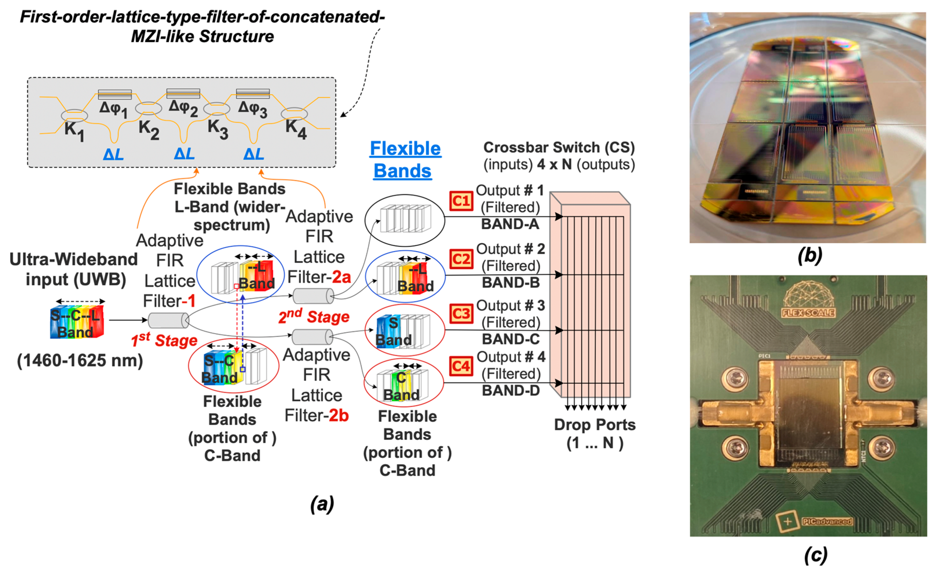
Figure 3.
Simulations results of cascaded adaptive filtering across (165 nm) spectrum defining four flexible bands for (a) FIR taps=20, (b) FIR taps=40.
Figure 3.
Simulations results of cascaded adaptive filtering across (165 nm) spectrum defining four flexible bands for (a) FIR taps=20, (b) FIR taps=40.
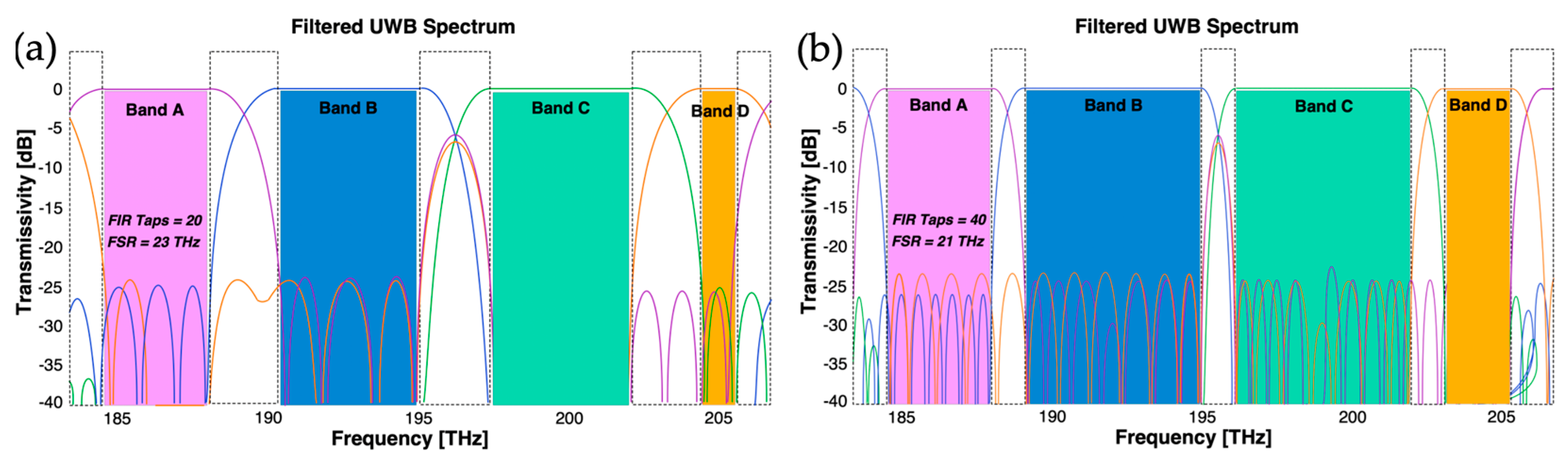
Figure 4.
(a) Conventional crossbar switch configuration of size 4×N (shown with N=6 output ports) lacks MZI at waveguide crossings. (b) Proposed Crossbar switch featuring waveguide crossings following every MZI aims to enhance performance as most MZIs are set to bar-state.
Figure 4.
(a) Conventional crossbar switch configuration of size 4×N (shown with N=6 output ports) lacks MZI at waveguide crossings. (b) Proposed Crossbar switch featuring waveguide crossings following every MZI aims to enhance performance as most MZIs are set to bar-state.
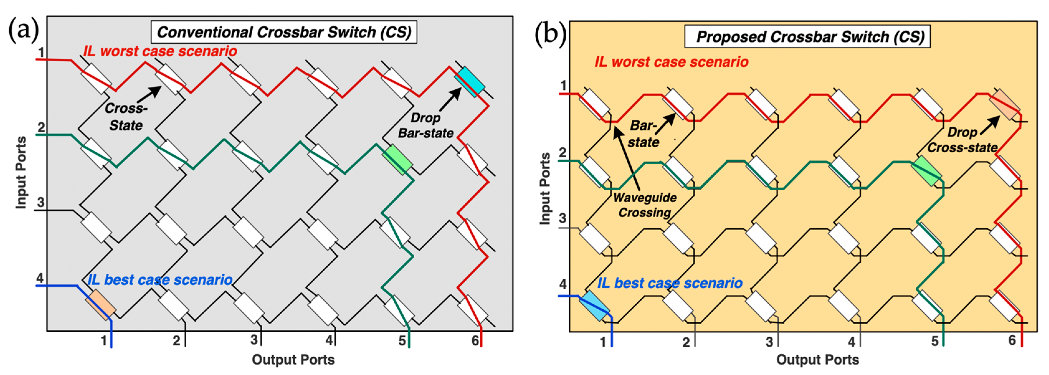
Figure 5.
Performance of (a) Stabilized DCs (50:50). (b) Single-stage FIRs with stabilized DC (50:50) and phase shifts. (c) Performance of CS switch for default cross||bar states.
Figure 5.
Performance of (a) Stabilized DCs (50:50). (b) Single-stage FIRs with stabilized DC (50:50) and phase shifts. (c) Performance of CS switch for default cross||bar states.
Figure 6.
OSNR as a function of traffic load highlights how OSNR decreases with increasing traffic load of MG-ON for different scenarios and spectral bands (S, C, L). The results highlight the impact of traffic allocation and loss mechanisms.
Figure 6.
OSNR as a function of traffic load highlights how OSNR decreases with increasing traffic load of MG-ON for different scenarios and spectral bands (S, C, L). The results highlight the impact of traffic allocation and loss mechanisms.
Figure 7.
BER vs Traffic Load for various scenarios and spectral bands (S, C, L) shows the impact of loss mechanisms and traffic distribution on signal quality, with higher BER indicating greater degradation under heavy traffic loads.
Figure 7.
BER vs Traffic Load for various scenarios and spectral bands (S, C, L) shows the impact of loss mechanisms and traffic distribution on signal quality, with higher BER indicating greater degradation under heavy traffic loads.
Figure 8.
Probability distributions (p) of the number of bands (top x-axis) and the corresponding number of guard bands (x) (bottom x-axis, up to n=3) under the binomial distribution, for different values of (S): (a) S=3, (b) S=6, (c) S=9 and (d) S=12.
Figure 8.
Probability distributions (p) of the number of bands (top x-axis) and the corresponding number of guard bands (x) (bottom x-axis, up to n=3) under the binomial distribution, for different values of (S): (a) S=3, (b) S=6, (c) S=9 and (d) S=12.
Figure 9.
Number of components and throughput for WBSS as a function of spatial lanes at different degrees of connectivity.
Figure 9.
Number of components and throughput for WBSS as a function of spatial lanes at different degrees of connectivity.
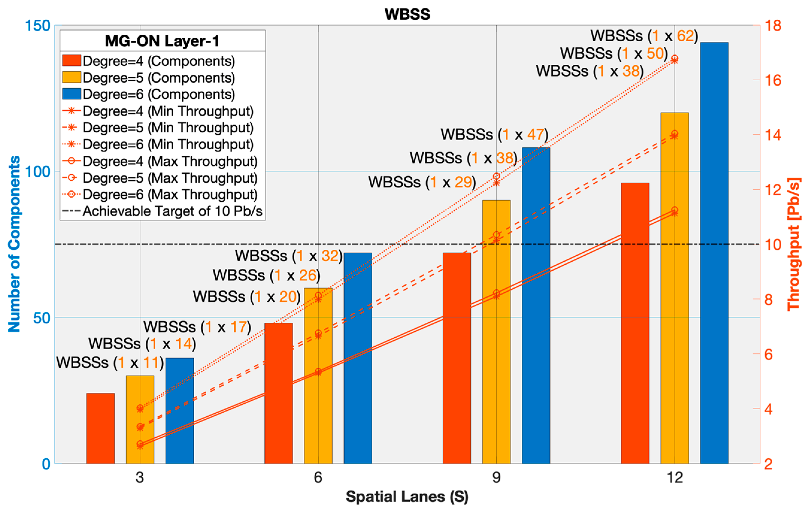
Figure 10.
Port count of components and throughput for INTER-OXC systems across various numbers of spatial lanes and degrees of connectivity.
Figure 10.
Port count of components and throughput for INTER-OXC systems across various numbers of spatial lanes and degrees of connectivity.
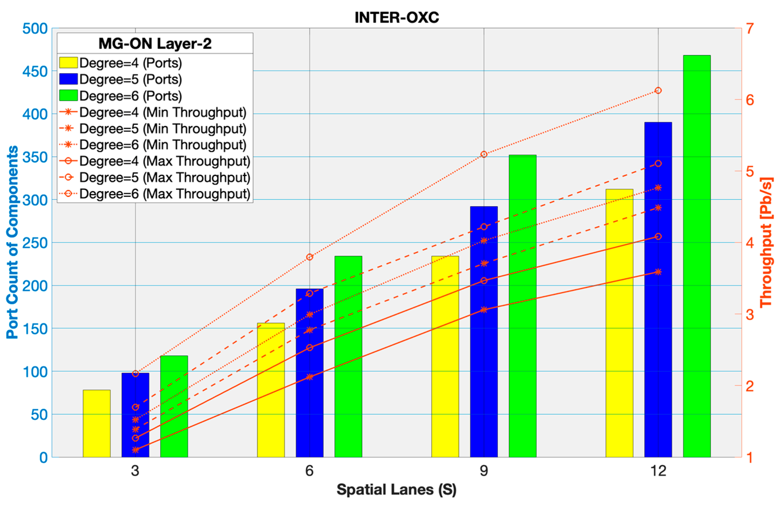
Figure 11.
Layer-2 throughput and number of band-transceivers across spatial lanes and degrees.
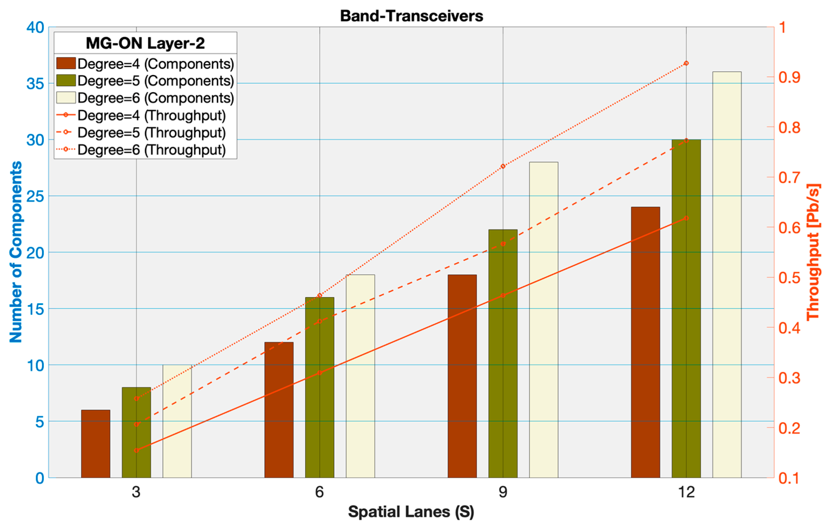
Figure 12.
MG-ON Relative Cost (Layers 1, 2) for various spatial lanes (S=2, 4, 6, 8) and Degrees (D= 3, 4, 5); (b) MG-ON vs Conventional and hybrid WSS-based architectures cost for D= (3, 4, 5).
Figure 12.
MG-ON Relative Cost (Layers 1, 2) for various spatial lanes (S=2, 4, 6, 8) and Degrees (D= 3, 4, 5); (b) MG-ON vs Conventional and hybrid WSS-based architectures cost for D= (3, 4, 5).
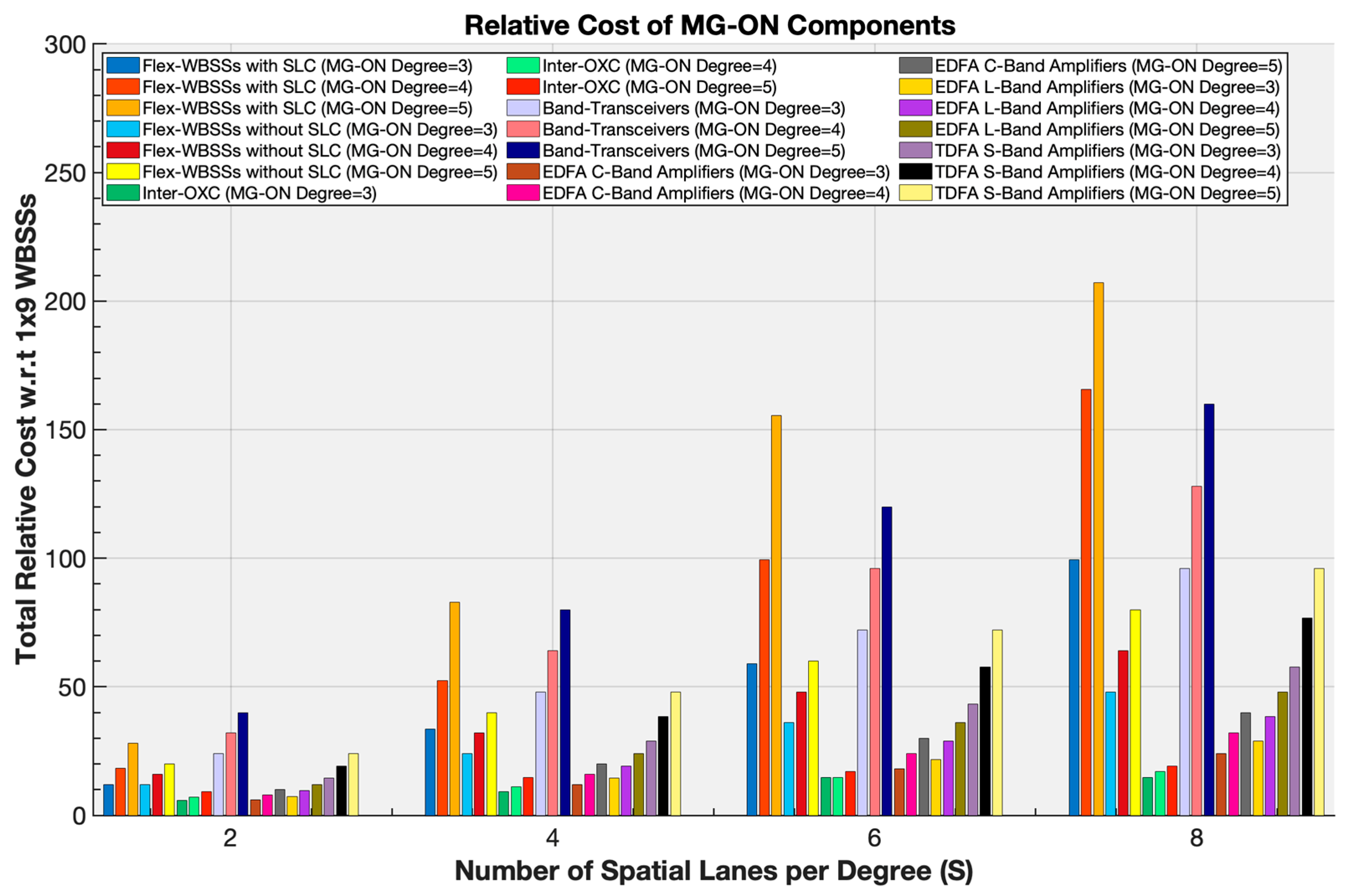
Figure 13.
Cost comparison of MG-ON (WBSS-based) and competitive WSS-based architectures for various spatial lanes (S = 2, 4, 6, 8) and degrees (D = 3, 4, 5).
Figure 13.
Cost comparison of MG-ON (WBSS-based) and competitive WSS-based architectures for various spatial lanes (S = 2, 4, 6, 8) and degrees (D = 3, 4, 5).
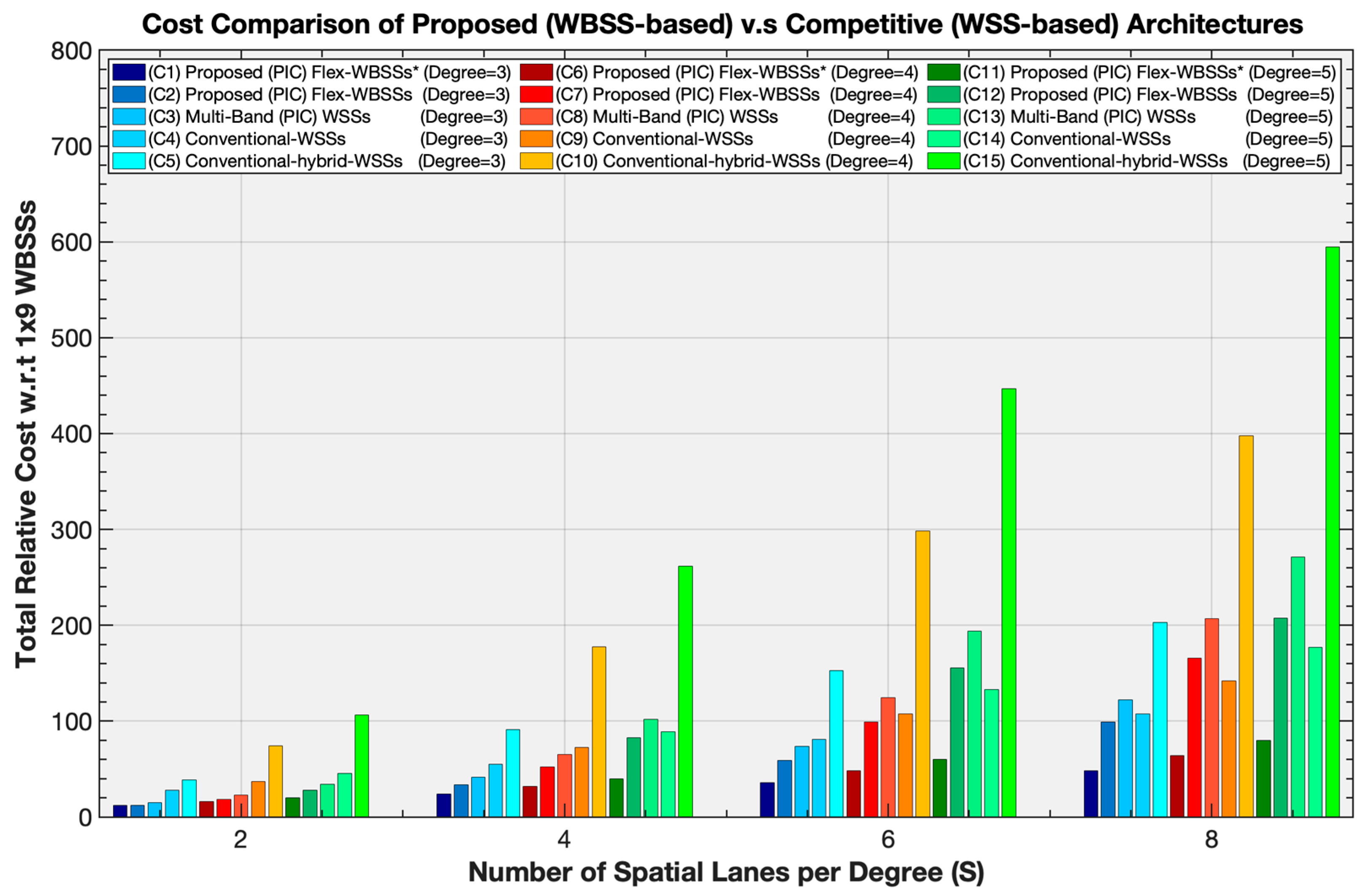
Figure 14.
Power consumption of control unit of (a) WBSSs with and without (SLC), (b) Inter-OXC and (c) Band-transceivers needed for realizing SDM nodes for three different MG-ON network scales (D=3, 4, 5), with varying numbers of spatial lane changes (S=2, 4, 6, 8).
Figure 14.
Power consumption of control unit of (a) WBSSs with and without (SLC), (b) Inter-OXC and (c) Band-transceivers needed for realizing SDM nodes for three different MG-ON network scales (D=3, 4, 5), with varying numbers of spatial lane changes (S=2, 4, 6, 8).
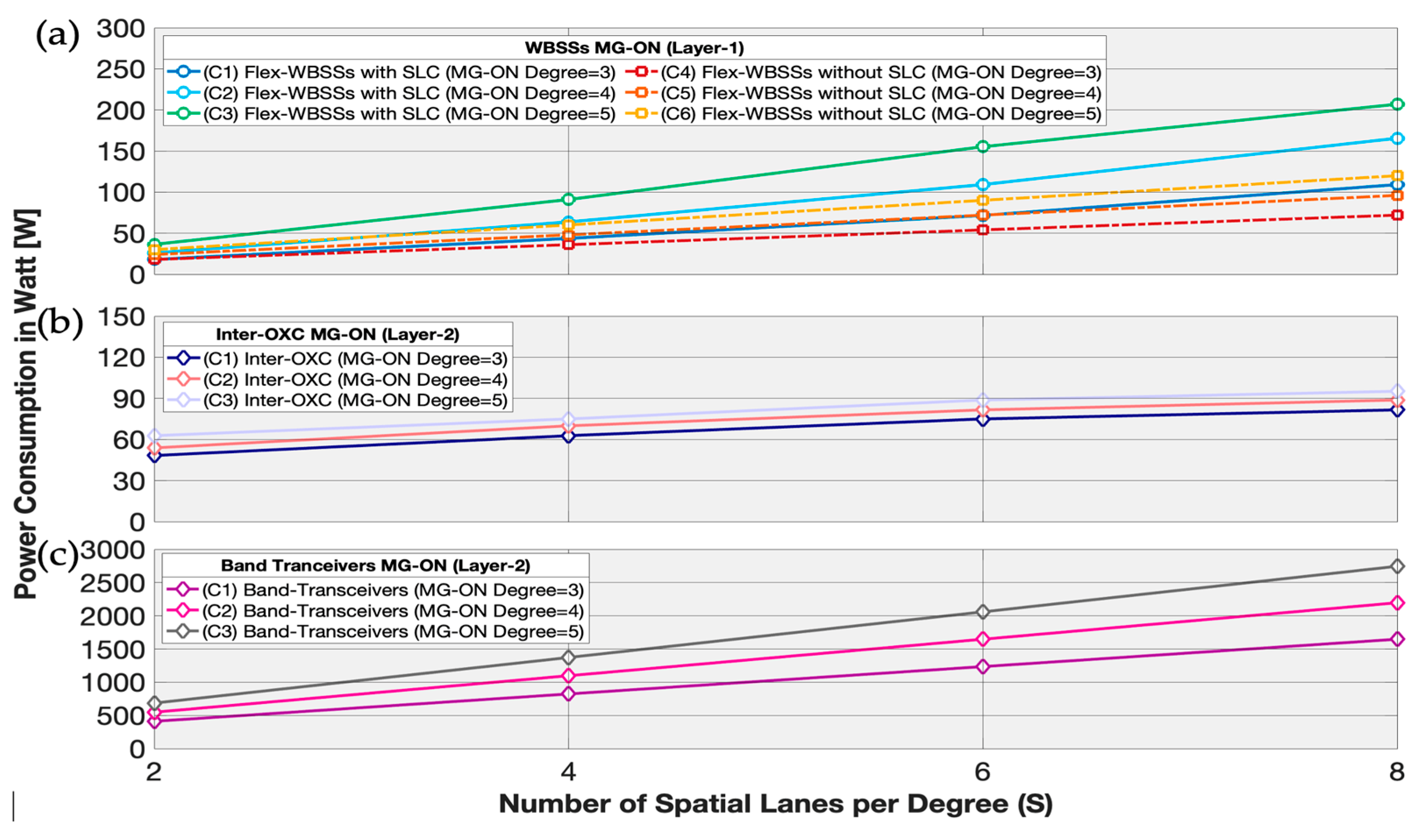

Table 1.
A description of node design parameters.
| Parameters | Description/Use |
| Spatial Lanes (S) | Seamlessly adapts from 3 to 9 spatial lanes ensuring compatibility with SDM technologies of high spatial parallelism. |
| Degree of Connectivity (D) | Investigating proper and efficient operation at varying degrees of connectivity (4, 5 and 6) simulating small, medium and large-scale nodes. |
| Inter-Layer Traffic (KB) | Supports add/drop 2 out of 4 available bands (KB=2) from/to Layer-1 to/from Layer-2, highlighting its multi-granular traffic switching. |
| For each element (Port Count) | Represents the count of both ingress and egress ports of each network element. |
| For each element (Total Number of components) | Represents the total number of components used for managing ingress /egress traffic. |
|
Guard Bands Bandwidth (GuardBW) |
Represents the transition bandwidth among (up to four) flexible bands ≈ 0.50 THz. |
| UWB Spectrum (UWBBW) | Represents the Ultra-Wide Band spectrum for (S+C+L) bands ≈ 21 THz. |
| Spectral Efficiency (SE) | Represents the spectral efficiency of band-transceivers ≈ 10.65 b/s/Hz. |
| Modulation Formats | QPSK and 16-QAM |
Table 2.
Derives the RC of all the MG-ON elements. All cost values are normalized to the cost of a 1×9 WBSS (Cost Unit CU ≈1).
Table 2.
Derives the RC of all the MG-ON elements. All cost values are normalized to the cost of a 1×9 WBSS (Cost Unit CU ≈1).
| Equipment | Cost Unit (CU) |
| Transceivers (single 600G) PIC | 8 |
| C-band EDFA | 0.5 |
| L-band EDFA | 0.6 |
| S-band TDFA | 1.2 |
| WBSS (PIC-based) [1×9] | 1 |
| WSS (PIC-based) [1×9] | 1.1 |
| WSS (Conventional) [1×9] | 2.2 |
| Inter-OXC [192×192] | 20 |
| Matrix-Switch [192×192] | 10 |
| OCS [192×192] | 16 |
| Band-MUX | 0.02 |
| Band-DEMUX | 0.02 |
Table 3.
Power Consumption Values for Basic MG-ON Switching Components (Layer 1-2).
| MG-ON Equipment (Nref) | Power Consumption (Pbase) |
| WBSS (PIC-based) [1×9] | 1.5 W |
| Inter-OXC [192×192] | 75 W |
| Band-Transceiver (multi-λ) | 13.81 W (single λ) |
Disclaimer/Publisher’s Note: The statements, opinions and data contained in all publications are solely those of the individual author(s) and contributor(s) and not of MDPI and/or the editor(s). MDPI and/or the editor(s) disclaim responsibility for any injury to people or property resulting from any ideas, methods, instructions or products referred to in the content. |
© 2025 by the authors. Licensee MDPI, Basel, Switzerland. This article is an open access article distributed under the terms and conditions of the Creative Commons Attribution (CC BY) license (http://creativecommons.org/licenses/by/4.0/).
Copyright: This open access article is published under a Creative Commons CC BY 4.0 license, which permit the free download, distribution, and reuse, provided that the author and preprint are cited in any reuse.


