Normalized Coefficient Linear Combinations (NCLC): A Unifying Framework for Discrete-Time Filters, Control, and Signal Analysis

1. Introduction

In engineering and applied mathematics, specifically within the domains of digital signal processing (DSP) and control theory, it is common to encounter expressions of the form

$$y=\sum _{i=1}^N{k}_i{f}_i,$$

where $f_i$ represents functions, signals, or sub-models, and the coefficients $k_i$ are subject to a normalization constraint

$$\sum _{i=1}^N{k}_i\left(x\right)=h\left(x\right),$$

for some carrier function h. Canonical examples include weighted averaging in numerical analysis, parallel signal paths in filter structures [1,2], and model blending in estimation and control.

The objective of this work is to formalize these structures as Normalized Coefficient Linear Combinations (NCLC). We propose this not as a new algorithm, but as a unified mathematical language to describe system behavior across disciplines. We show that:

• NCLC provides a consistent notation for systems in DSP, control, and numerical sequences.
• A simple normalization condition yields a general result regarding asymptotic preservation.
• In discrete-time LTI systems, normalization can be exploited as a design constraint to guarantee BIBO stability and DC gain simultaneously.

This perspective offers a structural approach to design, distinct from adaptive algorithms that update coefficients based on error minimization [3], focusing instead on invariant properties enforced by the normalization.

2. General NCLC Framework

2.1. Definition

Let X be a domain (e.g., $X=\mathbb{R}$ or $X=\mathbb{N}$), and let $f_i:X\to \mathbb{R}$, $i=1,\dots ,N$, be a set of basis functions or signals. Let $k_i:X\to \mathbb{R}$ be the coefficient functions.

Definition 1 (NCLC).

Given a carrier function $h:X\to \mathbb{R}$, the expression

$$y\left(x\right)=\sum _{i=1}^N{k}_i\left(x\right)f_i\left(x\right)$$

is a Normalized Coefficient Linear Combination (NCLC) with respect to h if and only if

$$\sum _{i=1}^N{k}_i\left(x\right)=h\left(x\right)forallx\in X.$$

The case $h\left(x\right)\equiv 1$ corresponds to a unitary normalization.

The carrier h encodes the global scale or asymptotic trend of the mixture, while the coefficients $k_i$ determine the local weighting of the branches $f_i$.

2.2. Asymptotic Preservation Properties

We now derive a proposition showing that NCLC structures preserve the asymptotic behavior of a reference trend.

Proposition 1 (Asymptotic preservation).

Let $f_{\mathrm{ref}}:X\to \mathbb{R}$ be a reference function such that $|f_{\mathrm{ref}}\left(x\right)|>0$ for all sufficiently large x. Suppose that for each i,

$$f_i\left(x\right)=f_{\mathrm{ref}}\left(x\right)\left(1+{\epsilon }_i\left(x\right)\right)$$

with ${\epsilon }_i\left(x\right)\to 0$ as $x\to \infty$. Assume that the coefficients $k_i\left(x\right)$ are bounded and satisfy the NCLC condition ${\sum }_{i=1}^N{k}_i\left(x\right)=h\left(x\right)$, where $h\left(x\right)$ is bounded away from zero for large x. Then

$$y\left(x\right)\sim h\left(x\right)f_{\mathrm{ref}}\left(x\right)(x\to \infty ).$$

Proof. 

Substituting the decomposition of $f_i$ gives

$$\begin{array}{cc}\hfill y\left(x\right)& =\sum _{i=1}^N{k}_i\left(x\right)f_{\mathrm{ref}}\left(x\right)\left(1+{\epsilon }_i\left(x\right)\right)\hfill \\ \hfill & =f_{\mathrm{ref}}\left(x\right)\sum _{i=1}^N{k}_i\left(x\right)\left(1+{\epsilon }_i\left(x\right)\right)\hfill \\ \hfill & =f_{\mathrm{ref}}\left(x\right)\left[\sum _{i=1}^N{k}_i\left(x\right)+\sum _{i=1}^N{k}_i\left(x\right){\epsilon }_i\left(x\right)\right]\hfill \\ \hfill & =f_{\mathrm{ref}}\left(x\right)\left[h\left(x\right)+\delta \left(x\right)\right],\hfill \end{array}$$

where

$$\delta \left(x\right):=\sum _{i=1}^N{k}_i\left(x\right){\epsilon }_i\left(x\right).$$

By boundedness of $k_i$ and ${\epsilon }_i\left(x\right)\to 0$, it follows that $\delta \left(x\right)=o\left(h\right(x\left)\right)$ as $x\to \infty$, provided $h\left(x\right)$ is bounded away from zero. Hence

$${\displaystyle \frac{y\left(x\right)}{h\left(x\right)f_{\mathrm{ref}}\left(x\right)}}=1+{\displaystyle \frac{\delta \left(x\right)}{h\left(x\right)}}⟶1,$$

which proves the asymptotic equivalence. □

3. Discrete-Time NCLC Systems

3.1. Design Theorem for LTI Systems

Standard discrete-time LTI systems are governed by the difference equation

$$y\left[n\right]=\sum _{i=1}^N{a}_{i}y[n-i]+\sum _{j=0}^M{b}_{j}x[n-j].$$

(1)

We can restate stability and gain conditions using the NCLC framework.

Theorem 1 (NCLC design constraint).

For the causal LTI system (1), suppose that:

1 

The feedback coefficients satisfy the contraction condition

$$\sum _{i=1}^N\left|a_i\right|<1;$$

2 

The input coefficients satisfy the normalization

$$\sum _{j=0}^M{b}_j=G_{\mathrm{dc}}\left(1-\sum _{i=1}^N{a}_i\right),$$

(2)

for some prescribed DC gain $G_{\mathrm{dc}}>0$.

Then the system is BIBO stable and its steady-state response to a step input of amplitude $X_0$ is exactly $y[\infty ]=G_{\mathrm{dc}}{X}_0$.

Proof. 

Stability follows from the absolute summability of the impulse response implied by condition 1 (the homogeneous recursion is a contraction; see [1]). For the steady-state value, consider a constant input $x\left[n\right]\equiv X_0$. For a BIBO-stable system, $y\left[n\right]\to Y_{\mathrm{ss}}$ exists, and taking limits in (1) yields

$$Y_{\mathrm{ss}}=\sum _{i=1}^N{a}_i{Y}_{\mathrm{ss}}+\sum _{j=0}^M{b}_j{X}_0,$$

so

$$Y_{\mathrm{ss}}\left(1-\sum a_i\right)=X_0\sum b_j.$$

Using (2), we obtain

$$Y_{\mathrm{ss}}={\displaystyle \frac{\sum b_j}{1-\sum a_i}}{X}_0=G_{\mathrm{dc}}{X}_0.$$

□

This theorem highlights that the sum of feedforward coefficients acts as a “carrier” normalizer for the DC gain, consistent with the NCLC interpretation.

4. Applications

4.1. First-Order NCLC Low-Pass Filter

The classic first-order recurrence

$$y\left[n\right]=ay[n-1]+(1-a)x\left[n\right],0<a<1,$$

(3)

is an explicit NCLC where $k_1=a$ and $k_2=1-a$, summing to $h\left[n\right]=1$. The carrier $h\equiv 1$ enforces a unit DC gain, independently of the pole location.

The impulse response of (3) is

$$h\left[0\right]=1-a,h\left[n\right]=(1-a)a^n,n\ge 0,$$

which is absolutely summable whenever $\left|a\right|<1$, guaranteeing BIBO stability.

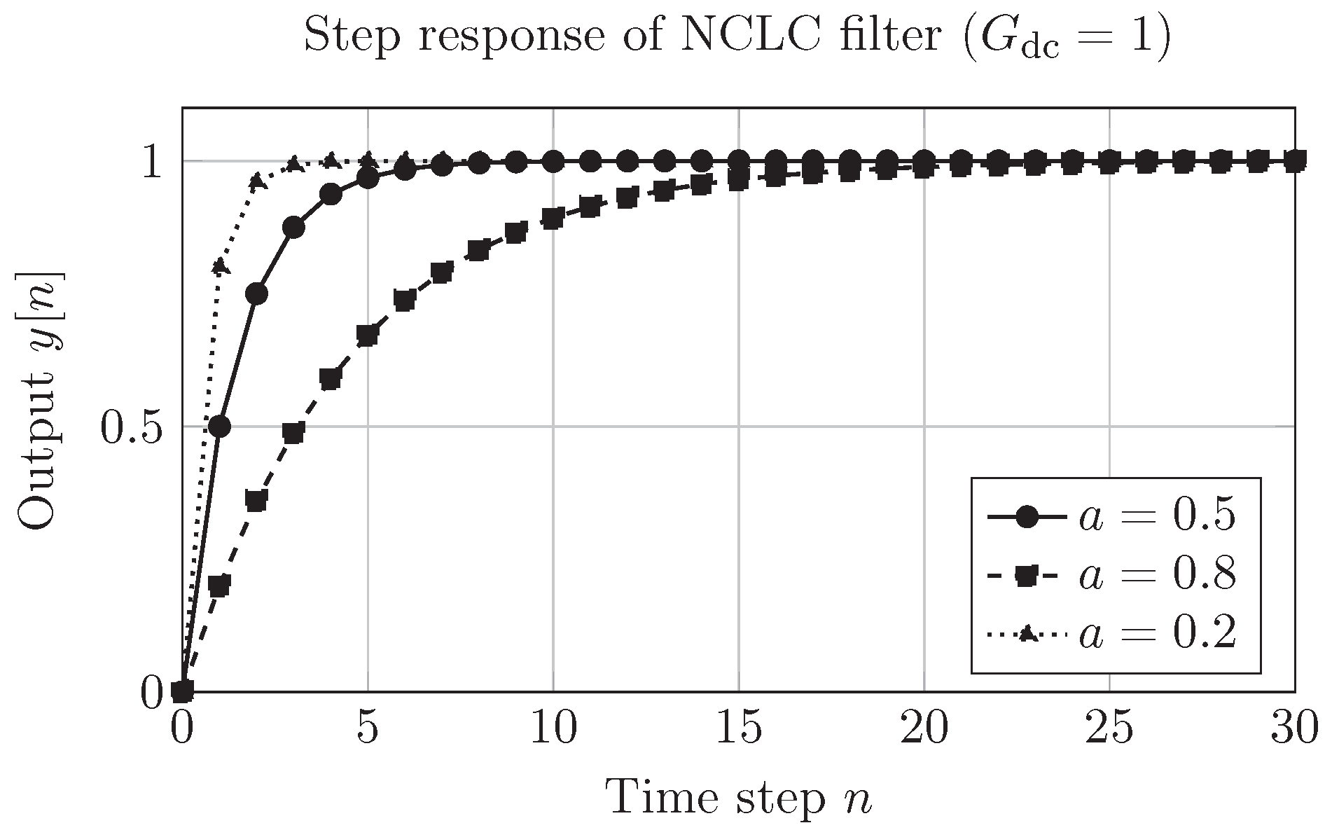
4.2. Step Response and Illustrative Simulation

Consider the unit-step input $x\left[n\right]=1$ for $n\ge 0$. For $\left|a\right|<1$, the step response of (3) is

$$y\left[n\right]=1-a^n,n\ge 0,$$

so all filters with $0<a<1$ converge to the same steady-state value $y[\infty ]=1$, but with different time constants. The NCLC normalization $a+(1-a)=1$ enforces the common carrier (unit DC gain), while tuning a changes only the dynamics.

Figure 1 shows the step response for three representative values of a. The plot is generated analytically using the above expression, but it can be interpreted as a simple discrete-time simulation.

4.3. Parametric Model Blending

In control, an adaptive mechanism might blend a nominal model $a_0$ with a corrected model $\widehat{a}$ through a normalized combination. For example, for the scalar system

$$x[n+1]=ax\left[n\right]+bu\left[n\right],y\left[n\right]=x\left[n\right],$$

one may consider a corrected model

$$\widehat{a}=a_0(1+\theta ),\widehat{x}[n+1]=\widehat{a}\widehat{x}\left[n\right]+bu\left[n\right],$$

with the parameter $\theta$ updated according to an error signal $e\left[n\right]=y\left[n\right]-\widehat{y}\left[n\right]$ via

$${\theta }_{n+1}={\theta }_n+\alpha e\left[n\right],0<\alpha \le 1.$$

At each step, the effective model blends the nominal contribution and a multiplicative correction controlled by $\theta$. This can be interpreted as an NCLC in parameter space, where the normalized combination balances nominal and corrective dynamics. A more detailed analysis of convergence conditions is left as future work.

5. Signal Analysis of Arithmetic Sequences

The NCLC framework can be extended to analyze numerical sequences by treating them as discrete-time signals. Consider the sequence of prime numbers $p_n$. From the prime number theorem, we know the asymptotic trend

$$p_n\sim nlogn$$

as $n\to \infty$ (see, e.g., [5]). Define the sequence

$$A_n:={\displaystyle \frac{nlogn}{p_n}}.$$

Then

$$A_n=1+{\epsilon }_n,{\epsilon }_n\to 0(n\to \infty ),$$

where ${\epsilon }_n$ can be interpreted as an “arithmetic noise” term in the approximation $p_n\approx nlogn$.

We can build an NCLC signal of the form

$$S_n=k_1\left(n\right)+k_2\left(n\right)A_n,$$

with normalization relative to a carrier $h\left(n\right)$:

$$k_1\left(n\right)+k_2\left(n\right)=h\left(n\right).$$

Substituting $A_n$,

$$S_n=h\left(n\right)+k_2\left(n\right){\epsilon }_n.$$

Proposition 2 (Growth-order preservation in a numerical NCLC).

Assume that $|{\epsilon }_n|\le C_{\epsilon }$ for all sufficiently large n, that $|k_2\left(n\right)|\le K$ is bounded, and that $h\left(n\right)\to \infty$ as $n\to \infty$. Then

$${\displaystyle \frac{S_n}{h\left(n\right)}}\to 1(n\to \infty ).$$

In particular, $S_n$ preserves the growth order of the carrier $h\left(n\right)$.

Proof. 

We have

$${\displaystyle \frac{S_n}{h\left(n\right)}}={\displaystyle \frac{h\left(n\right)+k_2\left(n\right){\epsilon }_n}{h\left(n\right)}}=1+{\displaystyle \frac{k_2\left(n\right){\epsilon }_n}{h\left(n\right)}}.$$

By assumption, $|k_2\left(n\right){\epsilon }_n|\le K{C}_{\epsilon }$, so

$$\left|{\displaystyle \frac{k_2\left(n\right){\epsilon }_n}{h\left(n\right)}}\right|\le {\displaystyle \frac{K{C}_{\epsilon }}{h\left(n\right)}}\to 0$$

as $n\to \infty$, since $h\left(n\right)\to \infty$. Thus $S_n/h\left(n\right)\to 1$. □

This suggests that techniques and intuition from signal filtering can be applied to smooth numerical sequences and recover asymptotic trends, with NCLC providing a structural language for doing so.

6. Conclusions

We have introduced the Normalized Coefficient Linear Combination (NCLC) as a unifying pedagogical and design framework. By explicitly separating the carrier (scale) from the constituent signals, NCLC simplifies the analysis of stability and gain in discrete-time LTI systems and offers a complementary perspective on numerical sequence analysis. The main contributions are:

• A general asymptotic-preservation result for NCLC structures.
• An NCLC-based design constraint for finite-order LTI systems, linking coefficient normalization to both BIBO stability and DC gain.
• Illustrative examples in first-order filtering, simple parametric model blending, and prime-based numerical signals.

Future work will investigate the application of NCLC in higher-order filter banks, constrained optimization for filter design, and nonlinear state estimation schemes where normalization constraints play a structural role.

References

- A. V. Oppenheim and A. S. Willsky, Signals and Systems, 2nd ed., Prentice Hall, Upper Saddle River, NJ, 1997.
- J. G. Proakis and D. K. Manolakis, Digital Signal Processing: Principles, Algorithms, and Applications, 4th ed., Pearson Prentice Hall, 2007.
- S. Haykin, Adaptive Filter Theory, 5th ed., Pearson Education, 2013.
- M. D. Kušljević and V. V. Vujičić, “Design of Digital Constrained Linear Least-Squares Multiple-Resonator-Based Harmonic Filtering,” Acoustics, vol. 4, no. 1, pp. 1–15, 2022. [CrossRef]
- T. M. Apostol, Introduction to Analytic Number Theory, Springer, New York, 1976.
Figure 1.
Step response of the NCLC filter . The coefficient normalization enforces the common steady-state value.
Disclaimer/Publisher’s Note: The statements, opinions and data contained in all publications are solely those of the individual author(s) and contributor(s) and not of MDPI and/or the editor(s). MDPI and/or the editor(s) disclaim responsibility for any injury to people or property resulting from any ideas, methods, instructions or products referred to in the content. |
© 2025 by the authors. Licensee MDPI, Basel, Switzerland. This article is an open access article distributed under the terms and conditions of the Creative Commons Attribution (CC BY) license (http://creativecommons.org/licenses/by/4.0/).
Copyright: This open access article is published under a Creative Commons CC BY 4.0 license, which permit the free download, distribution, and reuse, provided that the author and preprint are cited in any reuse.