Submitted:
20 November 2025
Posted:
21 November 2025
You are already at the latest version
Abstract
For the numerical simulation of rainwater infiltration in forest slope, information on the water retention curve (WRC), which shows spatial variability due to forest ecosystem and weathered granite in natural forest soils, is required. A scaling approach using three parameters of the LN model has been developed to simplify the spatial variability in the WRCs of forest slope of the soil under geomorphological process. This approach showed that we required spatial data set in scaling parameter, effective porosity, e, and each average value of remaining two parameters (the matric pressure head corresponding to the median pore radius, m, and the width of the pore-size distribution, ) which were defined as reference parameters. In this study, we estimated the minimum number of WRCs required to determine the reference parameters effectively. For this purpose, 77 WRCs of core samples were collected from whole 25 m forest slope, and we randomly sampled WRCs using a Monte Carlo simulation. The effect of scaling (EOS) increased with the sample size, and the increase became small at a sample size of approximately 20. We could explain 78% (EOS = 0.78) of spatial variability in the WRCs at the 95% confidence level by using the reference parameters derived from 8 samples. In addition, we performed stratified sampling to reduce the number of WRCs required. As a result, the sampling scheme, which considers the variability in only slope direction, was the most advantageous. This result indicated that the geomorphological process, which produces spatial variability in the reference parameters of forested slopes, is an important factor to effectively determine reference parameters. This paper concluded that scaling approach enables us to reduce the required number of samples for WRCs.
Keywords:
water retention curve
; Miller and Miller scaling
; reference parameter of scaling method
; required number of soil samples
; sampling strategy
1. Introduction
A quantitative assessment of rainwater infiltration into the soil is fundamental to evaluate the slope collapse caused by heavy rainfall in mountainous areas. The rainwater infiltration process was theoretically modeled and numerically simulated using the hydraulic properties of unsaturated soil, which were represented by the water retention curve (WRC) (the relationship between the volumetric soil water content, θ, and matric pressure head, ψ) and by unsaturated hydraulic conductivity. The WRC parameters are a part of the function of unsaturated hydraulic conductivity and are crucially important. These WRCs in drying path are formed by pore size distribution (Kosugi, 1996) show a large spatial variability within a natural forested slope (Hendrayanto et al., 1999; Pirastru et al., 2013).
However, it is usually not feasible to directly determine the spatial variability in the WRC from the sampling of soil on the entire forest slope and measurements in the laboratory because these studies are time-, labor-, and cost-intensive. Therefore, the hydraulic properties of unsaturated soils have been assumed to be homogeneous in many studies on the numerical simulation of rainwater infiltration (Hopp et al., 2009; Jana & Mohanty, 2012; Weiler & McDonnell, 2004). However, simulations assuming homogeneous soil cannot fully predict the actual water flow in the field (Sivapalan, 2003; Herbst et al., 2006).
To date, many studies have developed pedo-transfer function to predict WRC (Liao et al., 2014; Nguyen et al., 2015; Schaap et al., 2001; Wang et al., 2013). The pedo-transfer function could determine the WRCs easily. These methods require texture data, bulk density and organic matter content which require tiresome measurement and time.
A scaling technique was developed as an effective tool for simplifying the description of spatial variability in WRCs. The original scaling theory was introduced by Miller and Miller (1956), who derived the scaling theory using similar media theory. Scaling simplifications related WRCs at different spatial locations to a parameter called a scaling factor using the WRC of a set of reference parameters. Based on this concept, the microscopic structures of soils are assumed to be identical, and the soils differ only in their microscopic length scale, which is characterized by a scaling factor for each soil sample. This scaling technique is widely used in agricultural fields and grasslands (Ahuja et al., 1984; Eching et al., 1994). In contrast to soils in agricultural fields and grasslands, few studies have applied this technique to forest soils.
Kosugi and Hopmans (1998), indicated that ψm represents the microscopic length of the soil using the lognormal model, LN model (Kosugi, 1996), which contains three parameters (effective porosity, θe; matric pressure head corresponding to the median pore radius of pore-size distribution, ψm; and standard deviation of pore-size distribution, σ). Based on this finding, Hayashi et al. (2009) examined three parameters of the LN model to determine the parameters that characterize the spatial variability of WRCs on a natural forested slope. The results indicated that θe instead of ψm, mostly characterizes it. They proposed a new scaling approach that evaluates the spatial variability in WRCs using the spatial variability in θe. In this approach, θe was set as a scaling parameter that exhibits high spatial variability. At this time, the remaining two parameters showing small spatial variability (ψm and σ) were set as reference parameters and were identical within the forested slope.
For practical application of the scaling technique, a simple method for determining the scaling and reference parameters is needed. For this purpose, Nasta et al. (2009) proposed a simple application of a scaling technique based on a similar media theory. In their methods, WRCs were estimated from soil particle-size distribution data, whose measurement was much simpler than that of the WRC. They demonstrated that the spatial variability of WRCs can be characterized using the proposed method. To easily apply scaling approach to forest soils, Hayashi et al. (2009) calculated scaling parameter, θe as a difference between the water content observed at saturation and water content observed at ψ = −1000 cm, which is assumed equal to the residual water content. This method explained approximately 90% of the spatial variability in WRCs on the studied natural forested slope. Thus, the WRCs for the entire matric pressure range are not necessary for determining the scaling parameter.
However, little attentions have been paid to methods for determining reference parameters. Kosugi and Hopmans (1998) proposed a method in which the reference parameters are optimized by minimizing the residuals of volumetric water content, q. Several studies have used this method (Hendrayanto & Kosugi, 2000; Lakzaianpour et al., 2021; Sadeghi et al., 2016; Tuli et al., 2001). Deurer et al. (2001) derived the reference parameters from geometric means of their parameters. Chari et al. (2020) used an infiltration curve to determine the reference parameters, and Fred Zhang et al. (2004) estimated the reference parameters at the field scale through the inverse modeling of field experiments. Vishkaee et al. (2014) used reference parameter assuming that the reference soil is the one that consists of uniform-size spherical particles.
Most previous studies used a large number of WRCs and needed labor approaches to determine the reference parameters. They did not try to reduce the number of WRCs. However, because the values of the reference parameters are common within a site, it may be possible to determine them with high confidence from a small number of WRCs (Fred Zhang et al., 2004). In addition, in natural forested slopes, the soil structure characterizing the WRC is affected by forest biological activities, weathering, and geomorphological processes in Japan. Thus, there may be a spatial pattern in the spatial variability of the soil structure. Consequently, by recognizing the spatial pattern of the soil structure, we need to select the optimal sampling location to determine the reference parameters. This optimal sampling design for reference parameters, in combination with a simple determination of the scaling parameter proposed by Hayashi et al. (2009), reduces the required number of WRCs and allows us to save effort in measuring the enormous number of WRCs for describing the spatial variability in WRCs in a forested slope. Few studies have focused on the number of samples required to determine the hydraulic properties. Salemi et al. (2020) estimated an adequate number using statistical analysis. However, they analyzed the saturated hydraulic conductivity and not the water retention curves.
Therefore, the aim of this study is to establish the optimal sampling design for WRCs to identify reference parameters and facilitate the application of the scaling technique based on Hayashi et al. (2009) to forest soil. For this purpose, we statistically examined the accuracy of estimation of the WRCs to clarify how many samples are required to obtain these parameters and to suggest a sampling location that accounts for the effects of spatial distribution characteristics of WRCs in forest slope.
2. Materials and Method
2.1. Soil Sampling Location
The soil samples were taken from a natural forested slope (main and middle lower panels of Figure 1) underlain by the granitic bedrock (left upper panel of Figure 1) in the Tanakami Mountain range, Shiga Prefecture, Japan, situated at 34°55’00’’N and 135°58’58’’E. Detailed information on this site is provided by Hayashi et al. (2009).
We collected soil samples from vertically distributed profiles, as shown by Nh in Figure 1. Nh correlated with scaling parameter, qe (Hayashi et al., 2009), and reference parameters were not so correlated.
There was a small dip (indicated by an arrow in Figure 1) on the soil surface of the middle slope. There were slope regions with a thin soil layer below this dip and a thick soil layer above this dip. Thus, the dip may correspond to the head of an ancient landslide, and it was presumed that the thick soil layer consisted of debris brought by the landslide from the middle slope region. This was also supported by the vertical distribution of penetration resistance, Nh (Figure 1). Nh is the number of blows required for a 10-cm soil depth penetration, which was measured using a cone penetrometer with a 60° bit, cone diameter of 2 cm, weight of 2 kg, and fall distance of 50 cm. For Points b–d, the soil in the soil layer remained loose (Nh in the range of 0–20 blows/10 cm); however, the soil hardness on the bedrock increased rapidly and reached 100 blows/10 cm, which was the value observed at the interface between the soil layer and the bedrock. Such vertical distributions of Nh values are characteristic of a soil layer consisting of debris (Ousaka et al., 1992). Points e–h, which had a thin soil layer, were thought to be the residual soil remaining after the landslide. For the soils at points i–o, Nh gradually increased with depth. The soil layer indicating such a vertical distribution of Nh value was considered unaffected by the landslide (Ousaka et al., 1992).
Undisturbed soil samples were collected from 15 points distributed from the downslope (Point a) to upslope (Point o) segments to assess the spatial variability in the WRC on this forested slope (Figure 1). The sampling depths were set from the surface layer to the layer above the bedrock. The sampling locations are indicated by white dots in the panels in Figure 1. Soil samples were collected in triplicate at each point and depth. But, only at point j, we collected six samples at the depths of 15, 25, 35, 45, 55 cm and three samples at the depths of 2.5 and 75 cm.
2.2. Soil Sampling and Laboratory Experiments
Undisturbed soil samples were collected using thin-walled steel core samplers with a volume of 100 cm3 (5 cm inner diameter and 5.1 cm height). A sampler with a sharp edge was inserted vertically into the soil. Impact energy was applied to the cylinder using a hammer-driven device (DIK-1630; Dike Rika Kogyo, Tokyo, Japan). We followed the method described by Grossman and Reinsch (2002) to collect undisturbed soil samples and ensure sampling with minimum disturbance. The roots and organic material were carefully cut around the sampler during the insertion process.
Soil samples were transferred to aluminum trays in the laboratory. These were slowly saturated by wetting from the bottom over a 24 h period, and then weighed to determine the saturated water content, θs. Soil WRCs were then measured using the pressure plate method (Jury et al., 1991) for a matric pressure head, ψ, of −5, −10, −20, −30, −50, −70, –100, −200, −500, and −1000 cm. After measuring the water content at ψ = −1000 cm, each sample was oven-dried to determine the weight of soil in dry condition. The analyses described below were carried out using the average WRCs of three or six replicate samples (each with a volume of 100 cm3) collected at each point and depth. We analyzed the water retention characteristics of 77 soil samples.
There is a problem of hysteresis. The numerical simulation without hysteresis makes the matric potential head more widely fluctuated, compared with actual soil. However, because analysis including hysteresis is complicated, it is valid that in this study water retention curves of drying processes are analyzed using scaling method.
2.3. Water Retention Model
The LN model (Kosugi, 1996) is based on the assumption that the soil pore radius distribution obeys a lognormal distribution and expresses the WRC as
where θr and θs (cm3 cm-3) are the residual and saturated water contents, respectively; ψm (cm) is the matric pressure head corresponding to the median pore radius; σ represents the width of the pore-size distribution; and Q denotes the complementary normal distribution function defined as
The difference between θs and θr (i.e. θs − θr) is referred to as the effective porosity, θe.
A plot of Eq. [1] shown in Figure 2 demonstrates that ψm is the matric pressure head at the inflection point. The parameter σ is defined such that;
θ[ln(–ψm) − σ] − θ[ln(–ψm) + σ] = 0.68 × θe
Equation [3] shows that σ controls the magnitude of the change in θ around the inflection point. The parameter θe is defined by θs − θr, and represents the volumetric pore ratio effective for water storage.
2.4. Fitting of the LN Model
Prior to testing the proposed scaling methods, the observed WRC for each soil sample was fitted using the LN model (Fitting Approach IF; Individually Fitting). For ith soil sample, jth calculated water content, was calculated by applying the following equation using a nonlinear least squares optimization procedure (Wraith & Or, 1998):
where θr,i, θs,i, ψm,i and σi are the parameters for each soil sample i, ψj is the jth matric pressure head. To apply Eq. [4], for each soil sample, i, θr,i were fixed at water contents observed at ψ = −1,000 cm, θs,i was fixed to the observed saturated water content. As shown in Figure 3, slope of water retention curves at y = −1000 cm were almost 0. Therefore, we assumed q at y = −1000 cm was θr.
The parameters ψm,i and σi were optimized by minimizing the residual sum of squares (RSS) computed from
where J is the total number of data points for WRC of each soil sample (= 9), is the jth observed water content for a sample i, and is the calculated water content corresponding to . The sum of RSSi of all soil samples (RSSIF) was calculated as follows:
where, I is the total number of soil samples (= 77). This method provides the best description of the spatial variability in soil WRCs under the conditions assumed in the LN model.
In Fitting Approach UF (Universal Fitting), a single curve was applied to the entire data set with the LN model to exclude the spatial variability in all the parameters (ym, s, and qe) of the pore-size distribution function and a single set of parameters (i.e., and ) was optimized using
where is the jth water content calculated for sample i using Fitting Approach UF. The is shown in Figure 3. and were fixed to the arithmetic mean of all samples to apply Eq. [7]. The optimization procedure was conducted by minimizing RSSUF computed from
2.5. Scaling Method
Hayashi et al. (2009) indicated that, among the three parameters expressing the soil pore-size distribution (ψm, σ and θe), θe mostly characterizes the spatial variability in WRCs in natural forested slopes. Because θe is defined by the difference between θs and θr, they proposed a scaling approach in which θs and θr are set as scaling parameters differing for each soil, and the remaining two parameters (ψm and σ) are set as reference parameters identical within a study site). According to this scaling technique, WRC can be expressed as
where is the jth water content calculated for sample i using Eq. [9]. θr,i and θs,i are the residual and saturated water contents of the soil sample i, respectively. and are the reference parameters and are identical for the entire dataset.
Hayashi et al. (2009) suggested a scaling method that determines the scaling parameters θr,i and θs,i for each sample without using a dataset of WRCs, whose measurement requires enormous effort. In this method, θs,i is set to be observed θs for each soil, and θr,i is set to be the water content observed at ψ = −1000 cm for each soil, which was assumed to be equal to the residual water content θr. The reference parameters and were determined using optimization so that the parameters produced the best description of the entire dataset of WRCs for the entire slope. That is, Eq. [9] was applied to the whole dataset, and and were optimized using minimizing the residual sum of squares computed from
Using the whole dataset, I and J were 77 and 9, respectively.
2.6. Determination of Reference Parameters
If the universal reference parameters could be determined from a small number of WRCs without using the dataset of WRCs on the entire slope with acceptable confidence, effort in describing the spatial variability in WRCs on a forested slope would be reduced tremendously. We conducted a numerical experiment involving random sampling of WRCs by varying the sample size, n, using a Monte Carlo approach to examine the efficiency of the reference parameters derived from a limited number of WRCs. The procedure was as follows:
1) The first step was randomly selecting non-overlapping n WRC sets of WRCs among the 77 WRC datasets collected from the entire slope.
2) Reference parameters ( and ) were determined using n datasets of the selected WRCs. For this purpose, Eq. [9] was applied to n WRCs datasets and and were optimized by minimizing the RSS computed from Eq. [10]. θs,i was set to be observed θs for each soil, and θr,i was set to be the water content observed at ψ = −1,000 cm for each soil to apply Eq. [9]. The I and J in Eq. [10] were n and 9, respectively.
3) WRCs were described using the determined reference parameters. That is, the whole datasets of WRCs for the entire slope were computed by substituting one set of reference parameters ( and ) determined in Procedure 2 into Eq. [9]. The scaling parameters (difference between θs,i and θr,i) were set to the observed values for each sample i to apply Eq. [9]. The RSS of the estimated WRCs were calculated using Eq. [10]. In this case, I and J as expressed in Eq. [10] are n and 9, respectively. The accuracy of the scaling method was evaluated using the RSS values.
Procedures 1–3 were repeated 100,000 times for each assumed n value.
Scaling Approach demonstrated in Hayashi et al. (2009) corresponds to the case for sample size of 77 (i.e., n = 77).
2.7. Efficiency of Scaling Method
Using RSS by Eq. [10], the following two indices were computed to evaluate the accuracy of the scaling method: The coefficient of determination, R2, was calculated as
where is the arithmetic mean of the observed volumetric water content chosen in random sampling. R2 can be used to evaluate the performance of each scaling method by considering the variation in the observed θ values. In the proposed scaling method, I and J were equal to n and 9, respectively.
In addition to R2, considering the possible RSS range derived using the scaling method, the effect of scaling, EOS, was computed according to Hayashi et al. (2009):
Here, RSSIF represents the residual error when the spatial variability is most accurately expressed under the conditions in which the LN model is assumed. In contrast, RSSUF represents the error when the spatial variability in the pore-size distribution is not considered. Thus, EOS evaluates the effect of each scaling method by considering the possible range of RSS derived from the proposed scaling method. When the scaling method perfectly explains the spatial variation under the conditions in which the LN model is assumed, EOS is equal to one. In contrast, when the scaling method cannot explain spatial variability, EOS is equal to zero.
2.8. Semivariogram of Reference Parameters
We analyzed spatial distribution of reference parameters using semivariogram. The definition of semivariogram goes back to Matheron (1963). The experimental semivariograms of log(-ψm) and σ were calculated for the slope and vertical direction to assess the spatial pattern of log(-ψm) and σ in detail. The semivariogram function was computed as follows (Goovaerts, 1997):
where γ(h) is the semivariance, N(h) is the number of pairs of variables, z(xi) is the measured variable at spatial location xi, z(xi + h) is the measured variable at spatial location xi + h.
In general, the interval of the lag distance, h, is set to be constant; however, in the present study, N(h) is set to be constant to eliminate the bias of the number of data points (N(h) was fixed to 20 and 15 for the slope and vertical directions, respectively). In order to plot the γ(h), the arithmetic mean of the lag distance in each class was used to plot (h).
3. Result and Discussion
3.1. Observed Data and Efficiency of Fitting with the LN Model
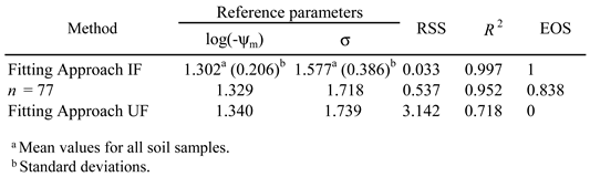
The 77 observed WRCs are shown in Figure 3. Figure 4 and Table 1 show the results of fitting the LN model to the WRCs. For Fitting Approach IF plots comparing the observed and calculated θ values were distributed close to the 1:1 line (Figure 4a), resulting in a very high R2 (0.997; Table 1) compared with n = 77 and Fitting Approach UF (Figure 4b and Figure 4c). This implied that the LN model performed well for each retention dataset at the study site.
Figure 5 shows spatial variabilities of reference parameters (log(-ψm) and σ) for each soil sample derived from Fitting Approach IF. Table 1 summarizes the arithmetic means and standard deviations. The log(-ψm) varied in the vertical direction without any clear trend, whereas there was a trend for the slope position: log(-ψm) in the middle and lower slope regions (Points b, c, and d) was smaller than the arithmetic mean 1.302 of for all data (Table 1), but in most areas of the upper slope region (Points e–o), log(-ψm) was greater than the arithmetic mean value. This might be because there are loose soils with large-sized pores from the middle slope region of the lower slope due to past landslides, as noted in the geomorphological processes in Figure 1. The σ for the slope direction has similar trends to log(-ψm); that is, at the lower slope region (points a through d), σ was greater than the arithmetic mean of 1.577 for all data (Table 1), but at the middle and upper slopes region (points e through o), σ was smaller than the arithmetic mean. In the vertical direction, σ varied slightly with depth, particularly at points i–o.
As mentioned above, the values of the two parameters differed between the lower and upper slope regions. Most likely, the soils in the lower part of the slope were composed of debris, and the soils in the upper part of the slope were composed of the material remaining after the landslide (Figure 1). Thus, log(-ψm) and σ may be affected by the topographic factor. The same trends of log(-ψm) and σ slope direction were observed by Hendrayanto et al. (1999) in forested granite slopes.
The fitted curve for the UF approach is shown in Figure 3. The plots comparing the observed and calculated θ values were widely scattered around the 1:1 line (Figure 4c). Hence, R2 for Fitting Approach UF (0.718) was much smaller than that for the Fitting Approach IF (0.997; Table 1).
The parameter log(-ψm) optimized using the Fitting Approach UF was similar to the arithmetic mean of log(-ψm) obtained using the Fitting Approach IF, whereas σ obtained using Fitting Approach UF was slightly greater than that obtained using the Fitting Approach IF (Table 1).
3.2. Effectivity of Scaling Using the Whole WRCs for Determination of Reference Parameters
This section confirmed the accuracy of the scaling method proposed by Hayashi et al. (2009) in which the reference parameters ( and ) were derived using the whole 77 data sets of WRCs (i.e., n = 77) in the entire forested slope. This accuracy corresponded to that of the case that produced the highest scaling effectiveness with optimal reference parameter values. As shown in Figure 4b, the plots for sample size of 77 comparing the observed and calculated θ values were distributed close to the 1:1 line with a high R2 (0.952; Table 1). EOS was 0.838, and this result indicated that the scaling method using the entire data sets of WRCs explained 83.8% of the total spatial variability in the WRCs. The value of log(-) optimized using this case was similar to that using the Fitting Approaches IF and UF (Table 1). In addition, the value of was similar to the value optimized using Fitting Approach UF.
Consequently, the scaling method could derive reference parameters that could describe the spatial variability in the WRCs for the studied forested slope. Therefore, we conclude that scaling can be conducted with high accuracy if the reference parameters are determined appropriately.
3.3. Relationship Between Effect of Scaling, EOS, and Reference Parameters and
Figure 6 presents the relationship between reference parameters log(-ψm) and σ optimized for each soil sample (i.e., case of sample size 1). This panel also shows isolines of EOS and the plot showing the highest EOS (i.e., EOS for a sample size of 77) determined in the previous subsection. This analysis of Figure 6 shows data to confirm how data of reference parameters distribute and how much EOS of each data of one WRC is, before main analysis, Montecarlo approach.
In Figure 6, the lengths of both axes were set such that the standard deviations of both reference parameters were of the same length on the panel. Hence, the shape of the isolines of EOS reflects the sensitivity of EOS to both reference parameters. It is clear from the figure that the EOS showed a concentric ellipse, whose widths were narrower in the direction of log(-) axis than in that of the axis. This shape indicated that the value of EOS was more sensitive to log(-) than .
In the following, we focus on the plots of the parameters log(-ψm) and σ, which correspond to the reference parameters when the sample size is one (i.e., n = 1). The plots of reference parameters were scattered widely around the highest EOS point, and it turned out that about 80% of the plots were in the area of EOS > 0.6. This proportion of plots corresponded to the confidence level of obtaining the EOS > 0.6 when we determined and by measuring WRC of one soil sample. In Figure 7, we show the cumulative relative frequency of the EOS values obtained when the sample size was 1 (i.e., n = 1). In this figure, the cumulative relative frequency represents the confidence level of obtaining an EOS value equal to or less than that indicated by the abscissa. At the 80% confidence level, EOS of 0.6 was obtained for the sample size of 1 (i.e., n = 1). Moreover, when a lower 60% confidence level was set, the obtained EOS increased to > 0.77.
3.4. Accuracy of Scaling Method for Different Sample Sizes
In this section, we present the results of a numerical experiment to examine the efficiency of the reference parameters derived from the WRCs selected using random sampling.
Figure 8 shows the plots of the reference parameters (log(- and ) for the sample sizes n = 3, 7, 8, 20, and 30, with the isolines of EOS. For each n value, sets of reference parameters were generated using Monte Carlo simulation. The figure shows the relative frequency for each grid in the log(-) and ranges. The cumulative frequency distribution curves for several sample sizes are shown in Figure 7.
As previously shown in Figure 6, the parameters exhibited large variations for a sample size of 1, and the EOS obtained at a high confidence level (e.g., 80%) was low (e.g., 0.6). Figure 8 shows that the plots of the parameters were concentrated around the point showing the highest EOS with an increase in sample size. According to this change, the cumulative relative frequency increased; that is, the EOS obtained at a given confidence level increased.
In Figure 9, we show how the scaling effect increases with the sample size at a given confidence level. Using this figure, we can investigate the number of samples required to obtain a sufficient EOS. By using only eight samples, one can attain an EOS > 0.78 at a 95% confidence level. The scaling modelling method developed by Hayashi et al. (2009) was applied successfully by reducing number of reference parameters. Salemi et al. (2020) proposed that the adequate sample size required to represent the spatial variability of the saturated hydraulic conductivity is approximately 20. The sample size of eight was much smaller than that estimated by Salemi et al. (2020).
We explained why our number of the necessary sample is widely smaller than that of Salemi et al. (2020). Salemi et al. (2020) did not analyze spatial variability of reference parameters, which showed small variability, but analyze large variability of saturated hydraulic conductivity. Furthermore, Salemi et al. (2020) and our study collected soils from different fields. Salemi et al. (2020)’s field was a 40-years old pasture, while our study’s field is forest slope.
3.5. Efficient Sampling Strategy
As previously mentioned, many samples are required using random sampling to obtain a high EOS when a high confidence level is set. It is expected that by conducting sampling at the optimal slope segment and soil layer, rather than random sampling, the required number of WRCs can be reduced. In this section, we evaluated the most effective sampling strategy for determining the reference parameters.
For this purpose, we conducted stratified instead of uniform random sampling to select WRCs. In the stratified sampling, 77 WRCs were divided into n strata according to their depths and horizontal points (Figure 10), and one WRC dataset was chosen randomly from each stratum, resulting in n samples.
We divided the population into the following strata: In Scheme 1, the population was divided into upper and lower slope segments, each of which was subdivided into n/2 soil layers (Figure 10a). In Scheme 2, the population was divided into surface and subsurface layers, each of which was subdivided into n/2 segments in the slope direction (Figure 10b). In Scheme 3, the population was divided into n segments along the slope direction (Figure 10c). Consequently, under the condition that the same sample size was set, Scheme 1 considered the variability for the vertical direction the most and for the forest slope direction the least, whereas Scheme 3 considered the variability for the vertical direction the least and for the slope direction the most.
Figure 11 presents the cumulative relative frequency of the EOS for Schemes 1, 2, and 3 for a sample size of 8 and for random sampling for sample sizes of 8 and 10. Each of the three stratified sampling schemes performed better than random sampling for the same sample size of eight. Among the three schemes, the cumulative frequency was the highest in Scheme 3, lower in Scheme 2, and lowest in Scheme 1, respectively. The cumulative frequency for Scheme 3 was comparable to that for random sampling for a sample size of 10. Therefore, Scheme 3 could reduce the sample size by two to obtain the same EOS in comparison to the case in which no sampling strategy was introduced.
3.6. Semivariogram of Reference Parameters
Scheme 3, which considered the variability for the slope direction most greatly, was most advantageous among the three schemes, whereas Scheme 1, which mostly considered the variability for the vertical direction, was least advantageous. This result suggested that the values of reference parameters had larger variability for the forest slope direction than for the vertical direction. In fact, both log(-ψm) and σ showed this trend in Figure 5. Note that this does not necessarily indicate that the WRC exhibits larger variability for the slope direction than for the vertical direction because the spatial variability of WRC was characterized more greatly by the scaling parameter than by the reference parameters.
Figure 12 shows the calculated semivariogram (Eq. [13]). The semivariance of the log(-ψm) for the slope direction had small nugget and was as large as the variance of all samples at the lag distance of 1.7 m (Figure 12a). Because the average sampling interval for the slope direction is 1.8 m, this result indicated that there were many adjacent pairs in the slope direction that had a small correlation in the log(-ψm) value. The same is true σ for the slope direction (Figure 12c). That is, the semivariance of the σ for the slope direction reached the variance of all samples at the lag distance < 1.8 m. For the vertical direction, both semivariance of log(-ψm) and σ did not show a larger value than nugget (Figure 12b and Figure 12d).
Consequently, both reference parameters varied more in the slope direction than in the vertical direction. For both parameters, there was little correlation between the values of adjacent pairs in the slope direction. Therefore, it was led to the result that Scheme 3 performed best. It is crucial to collect samples from different slope segments differentiated by geomorphological processes to determine the reference parameters for a naturally forested slope.
4. Conclusion
We estimated the number of WRCs required to determine the reference parameters ( m and ) to effectively apply the scaling technique proposed for forest soil (Hayashi et al., 2009). For this purpose, we implemented random sampling of the WRCs collected from an entire forested slope by varying the sample size using the Monte Carlo method. As a result, in the figure of relationship between log(- m) and s, isolines of EOS were distributed concentrically. The highest EOS calculated from the whole 77 data sets of reference parameters was plotted at the center of the figure. In addition, as sample number of WRCs required to determine reference parameters was larger, the probability of deriving the highest EOS was greater. The effect of scaling increased with increasing sample size. Its rate of increase decreased and became about 0 at a sample size of approximately 20. 78% of the spatial variability of the WRCs was explained at a 95% confidence level by using the reference parameters derived from eight samples.
Stratified sampling was performed to reduce the number of WRCs required with a high EOS. Three sampling schemes were tested by considering the different spatial patterns to investigate the effective stratified sampling. The sampling scheme that considered the variability in the slope direction but not in the vertical direction was the most advantageous. The reference parameters derived from eight samples using this scheme performed the accuracy of ten samples derived from complete random sampling. This result suggested that the spatial variability in the reference parameters is affected by geomorphological processes. Here, geomorphological processes mean an ancient landslide on the studied slope caused a thick soil layer in the downslope region consisting of debris brought from the middle slope region, and the middle and upper slope regions contained the remaining soils. We found that such geomorphological processes had a governing effect on determination of reference parameters.
We should describe the unsaturated hydraulic conductivity. LN model functionalized unsaturated hydraulic conductivity using parameters of saturated hydraulic conductivity and two parameters ( ;m and ). Here, the two parameters correspond to the reference parameters used in this study. Hayashi et al. (2009) insisted that reference parameters can be set to be homogeneous based on soil pore structure. Therefore, it is highly possible to assume that two parameters are homogeneous when we express unsaturated hydraulic conductivity.
In this study, we investigated datasets obtained from a steep forested slope underlain by weathered granite. Future studies should examine the applicability of the proposed scaling technique to slopes under different geomorphological, vegetative, and geological conditions.
Abbreviations
EOS, Effect of Scaling;
LN model, lognormal model;
RSS, residual sum of squares;
WRC, water retention curve
References
- Ahuja, L. R., Naney, J. W., & Nielsen, D. R. (1984). Scaling soil-water properties and infiltration modeling. Soil Science Society of America Journal, 48(5), 970–973. [CrossRef]
- Chari, M. M., Poozan, M. T., & Afrasiab, P. (2020). Modeling soil water infiltration variability using scaling. Biosystems Engineering, 196, 56–66. [CrossRef]
- Deurer, M., Duijnisveld, W. H. M., Böttcher, J., & Klump, G. (2001). Heterogeneous solute flow in sandy under a pine forest: Evaluation of a modeling concept. Journal of Plant Nutrition and Soil Science, 164(6), 601–610. [CrossRef]
- Eching, S. O., Hopmans, J. W., & Wallender, W. W. (1994). Estimation of in-situ unsaturated soil hydraulic functions from scaled cumulative drainage data. Water Resources Research, 30(8), 2387–2394. [CrossRef]
- Fred Zhang, Z. F., Ward, A. L., & Gee, G. W. (2004). A parameter scaling concept for estimating field-scale hydraulic functions of layered soils. Journal of Hydraulic Research, 42, sup1, 93–103. [CrossRef]
- Goovaerts, P. (1997). Geostatistics for Natural Resources Evaluation Oxford University Press.
- Grossman, R. B., & Reinsch, T. G. (2002). Core method. In A. Klute (Ed.), Methods of soil analysis. Part 4- Physical Methods. Monograph 9 (pp. 207–209). ASA and SSSA.
- Hayashi, Y., Kosugi, K., & Mizuyama, T. (2009). Soil water retention curves characterization of a natural forested hillslope using a scaling technique based on a lognormal pore-size distribution. Soil Science Society of America Journal, 77, 55–64.
- Hendrayanto, K., & Kosugi, T. Mizuyama. (2000) Scaling hydraulic properties of forest soils, Hyrol. Process., 14, 521–538.
- Hendrayanto, K., Kosugi, T., & Uchida, S. Matsuda, and T. Mizuyama. (1999). Spatial variability of soil hydraulic properties in a forested hillslope. Japan forest research 4:107-114.
- Herbst, M., Diekkrüger, B., & Vanderborght, J. (2006). Numerical experiments on the sensitivity of runoff generation to the spatial variation of soil hydraulic properties. Journal of Hydrology, 326(1–4), 43–58. [CrossRef]
- Hopp, L., Harman, C., Desilets, S. L. E., Graham, C. B., McDonnell, J. J., & Troch, P. A. (2009). Hillslope hydrology under glass: Confronting fundamental questions of soil-water-biota co-evolution at Biosphere 2. Hydrology and Earth System Sciences, 13(11), 2105–2118. [CrossRef]
- Jana, R. B., & Mohanty, B. P. (2012). On topographic controls of soil hydraulic parameter scaling at hillslope scales. Water Resources Research, 48(2), W02518. [CrossRef]
- Jury, W. A., Gardner, W. R., & Gardner, W. H. (1991). Soil Physics Wiley. New York.
- Kosugi, K. (1996). Lognormal distribution model for unsaturated soil hydraulic properties. Water Resources Research, 32(9), 2697–2703. [CrossRef]
- Kosugi, K., & Hopmans, J. W. (1998). Scaling water retention curves for soil with lognormal pore-size distribution. Soil Science Society of America Journal, 62(6), 1496–1505. [CrossRef]
- Lakzaianpour, G. H., Chari, M. M., Tabatabaei, S. M., & Afrasiab, P. (2021). Scaling lognormal water retention curves for dissimilar soils. Hydrological Sciences Journal, 66(4), 622–629. [CrossRef]
- Liao, K., Xua, F., Zheng, J., Zhu, Q., & Yang, G. (2014). Using different multimodel ensemble approaches to simulate soil moisture in a forest site with six traditional pedotransfer functions. Environmental Modelling and Software, 57, 27–32. [CrossRef]
- Miller, E. E., & Miller, R. D. (1956). Physical theory for capillary flow phenomena. Journal of Applied Physics, 27(4), 324–332. [CrossRef]
- Nasta, P., Kamai, T., Chirico, G. B., Hopmans, J. W., & Romano, N. (2009). Scaling soil water retention functions using particle-size distribution. Journal of Hydrology, 374(3–4), 223–234. [CrossRef]
- Nguyen, P. M., De Pue, J. D., Le, K. V., & Cornelis, W. (2015). Impac of regression methods onimproved effect of soil structure on soil water retention estimates. Journal of Hydrology, 525, 598–606. [CrossRef]
- Ousaka, O., Tamura, T., Kubota, J., & Tsukamoto, Y. (1992). Survey of developing processes of soil layer in a granitic hillslope (in Japanese with English abstract). Journal of the Japan Society of Erosion Control. Engeering, 43, 3–12.
- Pirastru, M., Castellini, M., Giadrossich, F., & Niedda, M. (2013). Comparing the hydraulic properties of forested and grassed soils on an experimental hillslope in a Mediterranean environment. Procedia Environmental Sciences, 19, 341–350. [CrossRef]
- Sadeghi, M., Ghahraman, B., Warrick, A. W., Tuller, M., & Jones, S. B. (2016). A critical evaluation of the Miller and Miller similar media theory for application to natural soils. Water Resources Research, 52(5), 3829–3846. [CrossRef]
- Salemi, L. F., Fernandes, R. P., Silva, R. W. C., Garcia, L. G., de Moraes, J. M., Groppo, J. D., & Martinelli, L. A. (2020). Soil hydraulic properties: A simple and practical approach to estimate the number of samples. Eurasian Journal of Soil Science, 9(1), 18–23. [CrossRef]
- Schaap, M. G., Leij, F. J., & van Genuchten, M. T. (2001). Rosetta: A computer program for estimating soil hydraulic parameters with hierarchical pedotransfer functions. Journal of Hydrology, 251(3–4), 163–176. [CrossRef]
- Sivapalan, M. (2003). Prediction in ungauged basins: A grand challenge for theoretical hydrology. Hydrological Processes, 17(15), 3163–3170. [CrossRef]
- Tuli, A., Kosugi, K., & Hopmans, J. W. (2001). Simultaneous scaling of soil water retention and unsaturated hydraulic conductivity functions assuming lognormal pore-size distribution. Advances in Water Resources, 24(6), 677–688. [CrossRef]
- Vishkaee F. M., M. H. Mohammadi, & M. Vanclooster (2014). Predicting the soil moisture retention curve, from soil particle size distribution and bulk density data using a packing density scaling factor. Hydrol. Earth Syst. Sci., 18, 4053–4063. doi:10.5194/hess-18-4053-2014.Wang, C., Zhao, C. Y., Xu, Z. L., Wang, Y., & Peng, H. H. (2013). Effect of vegetation on soil water retention and storage in a semi-arid alpine forest catchment. Journal of Arid Land, 5(2), 207–219. [CrossRef]
- Weiler, M., & McDonnell, J. (2004). Virtual experiments: A new approach for improving process conceptualization in hillslope hydrology. Journal of Hydrology, 285(1–4), 3–18. [CrossRef]
- Wraith, J. M., & Or, D. (1998). Nonlinear parameter estimation using spread sheet softwater. Journal of Natural Resources and Life Sciences Education, 27(1), 13–19. [CrossRef]
Figure 1.
Photo, topography and longitudinal section of the natural forested slope showing the locations of soil sampling Points a–o. Values of Nh represent the number of blows required for a 10-cm penetration using a cone penetrometer with a 60-bit, a cone diameter of 2 cm, a weight of 2 kg, and a fall distance of 50 cm. White dots on the longitudinal section indicate the sampling locations.
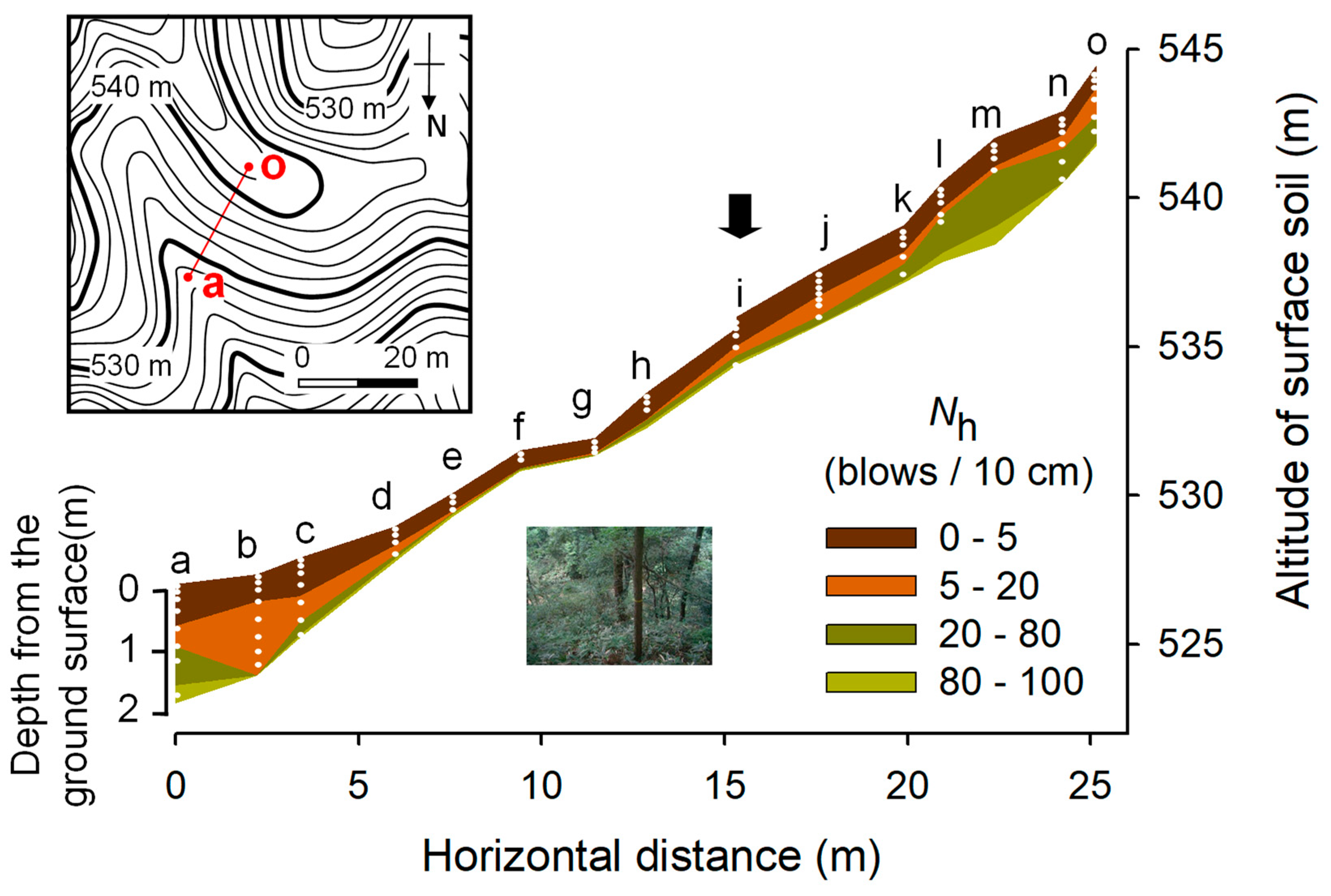
Figure 2.
Schematic representation of the water retention curve (WRC), based on the LN model represented in Eq. [1].
Figure 2.
Schematic representation of the water retention curve (WRC), based on the LN model represented in Eq. [1].
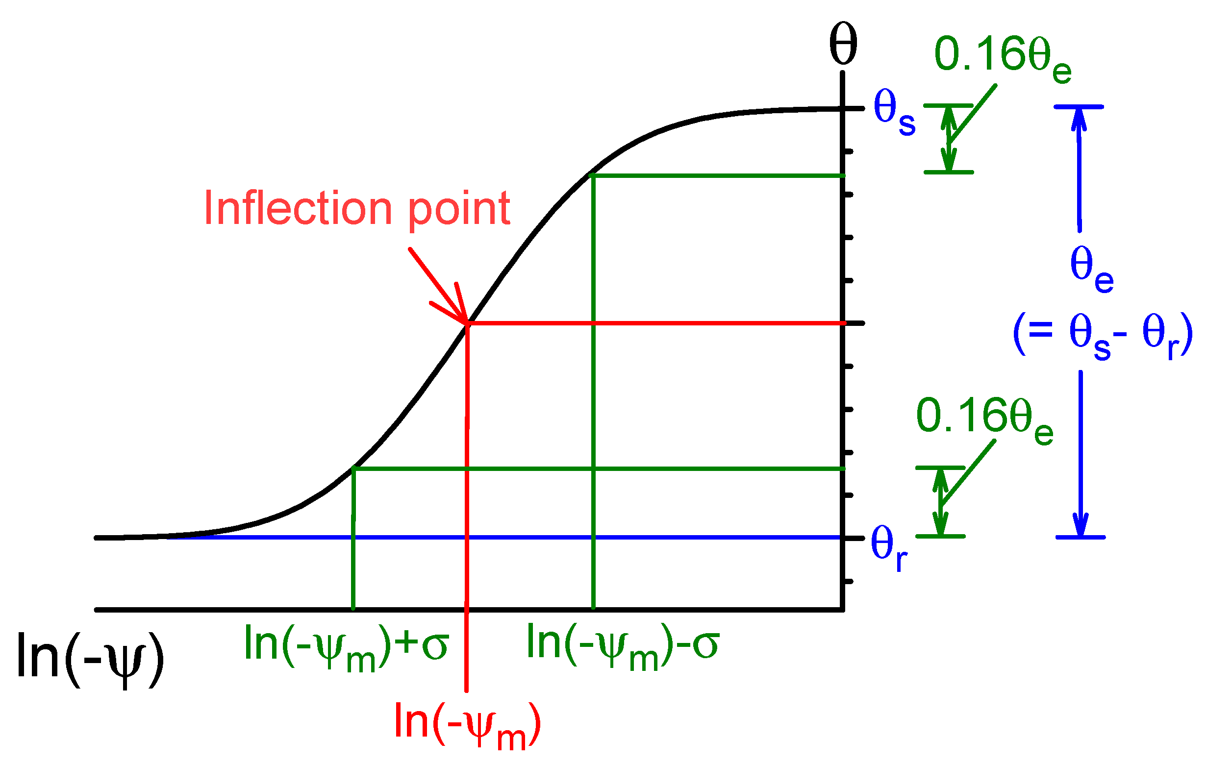
Figure 3.
Observed 77 water retention curves (WRCs) for all soil samples and red curve fitted using Fitting Approach UF (i.e. Eq. [7]).
Figure 3.
Observed 77 water retention curves (WRCs) for all soil samples and red curve fitted using Fitting Approach UF (i.e. Eq. [7]).
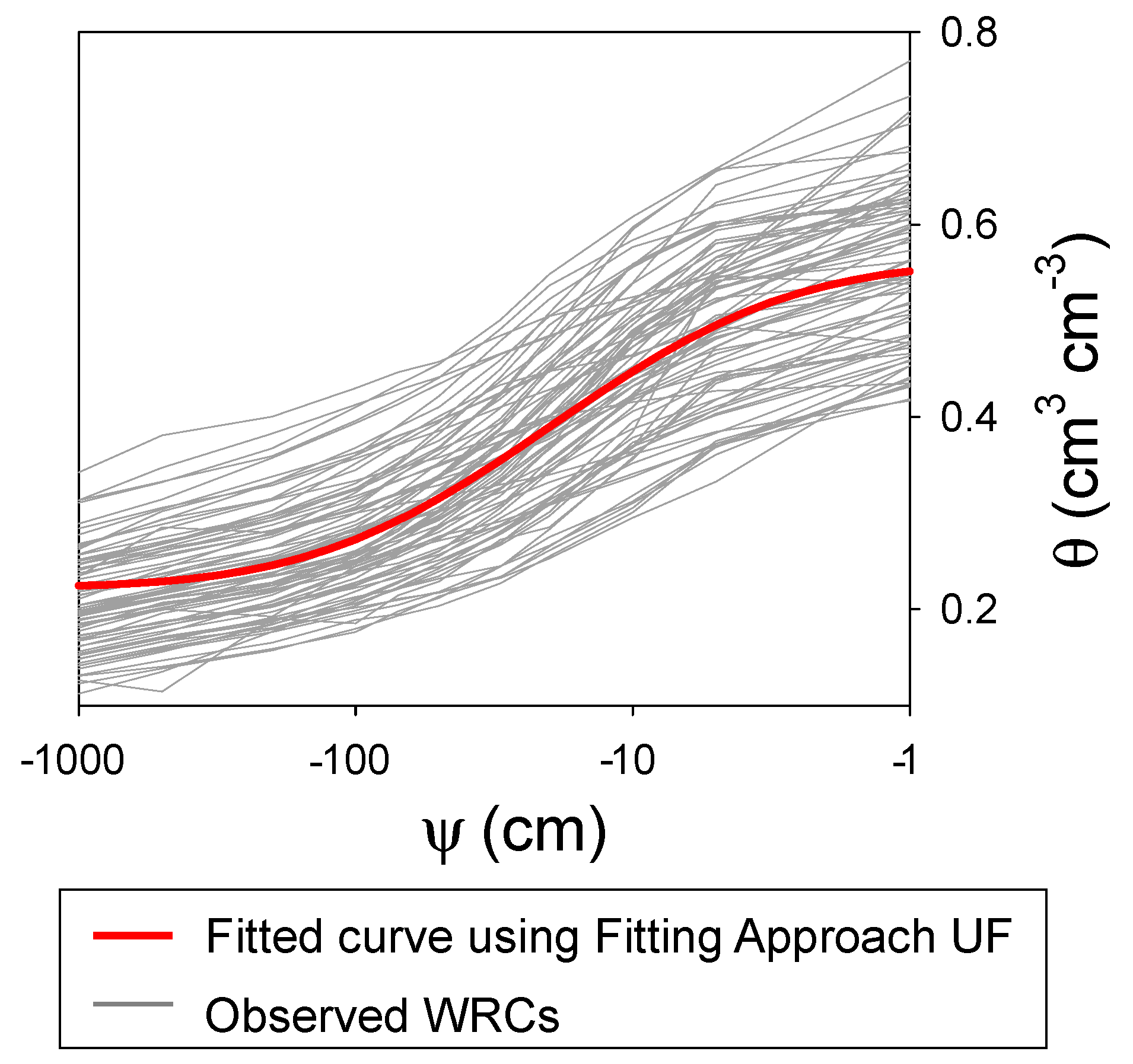
Figure 4.
Comparison between observed water content qobs and calculated water content qcal using (a) Fitting Approach IF, (b) scaling method for sample size of 77, and (c) Fitting Approach UF.
Figure 4.
Comparison between observed water content qobs and calculated water content qcal using (a) Fitting Approach IF, (b) scaling method for sample size of 77, and (c) Fitting Approach UF.
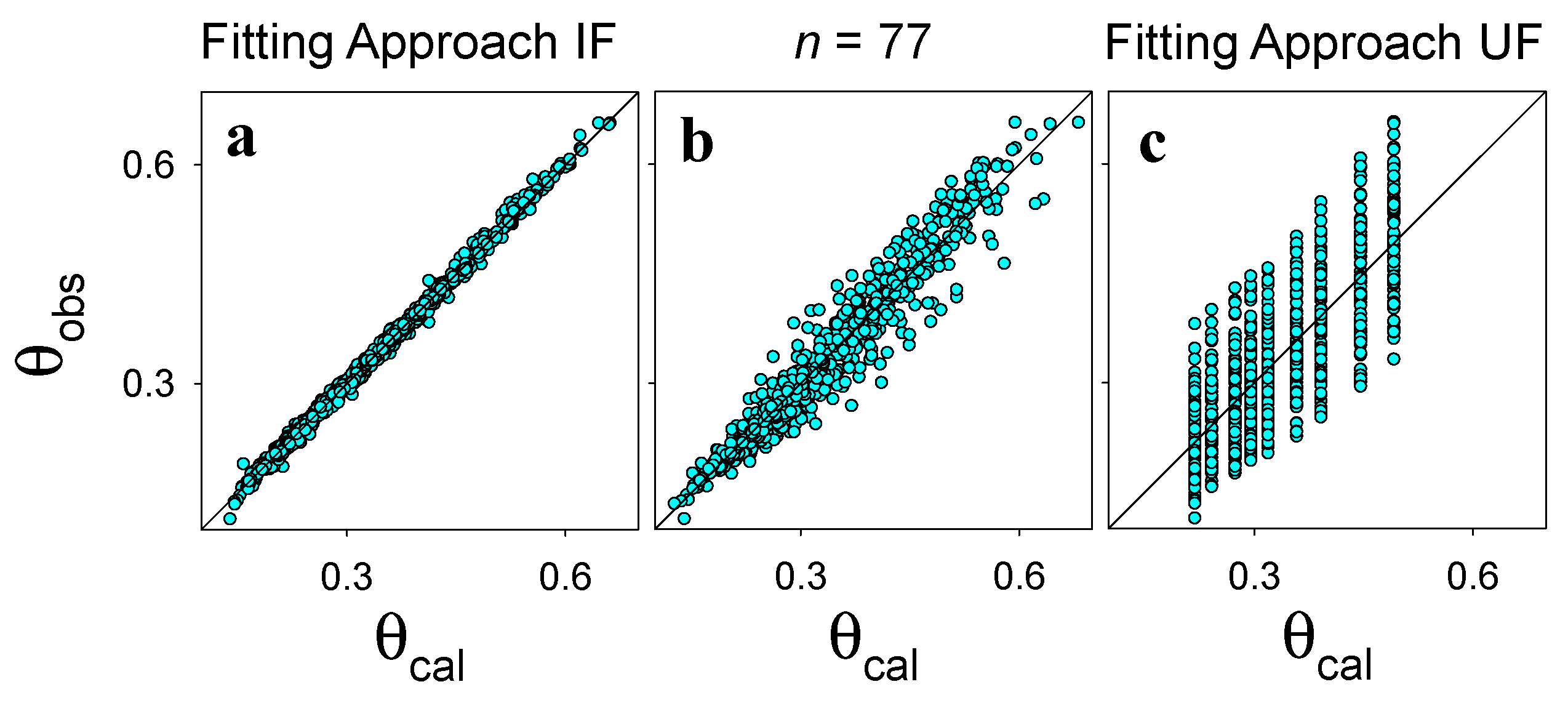
Figure 5.
Spatial variability of refence parameters, log(-ym) and s of observed 77 water retention curves (WRCs) for all soil samples on the studied forested slope. Small open circles indicate the sampling depths.
Figure 5.
Spatial variability of refence parameters, log(-ym) and s of observed 77 water retention curves (WRCs) for all soil samples on the studied forested slope. Small open circles indicate the sampling depths.
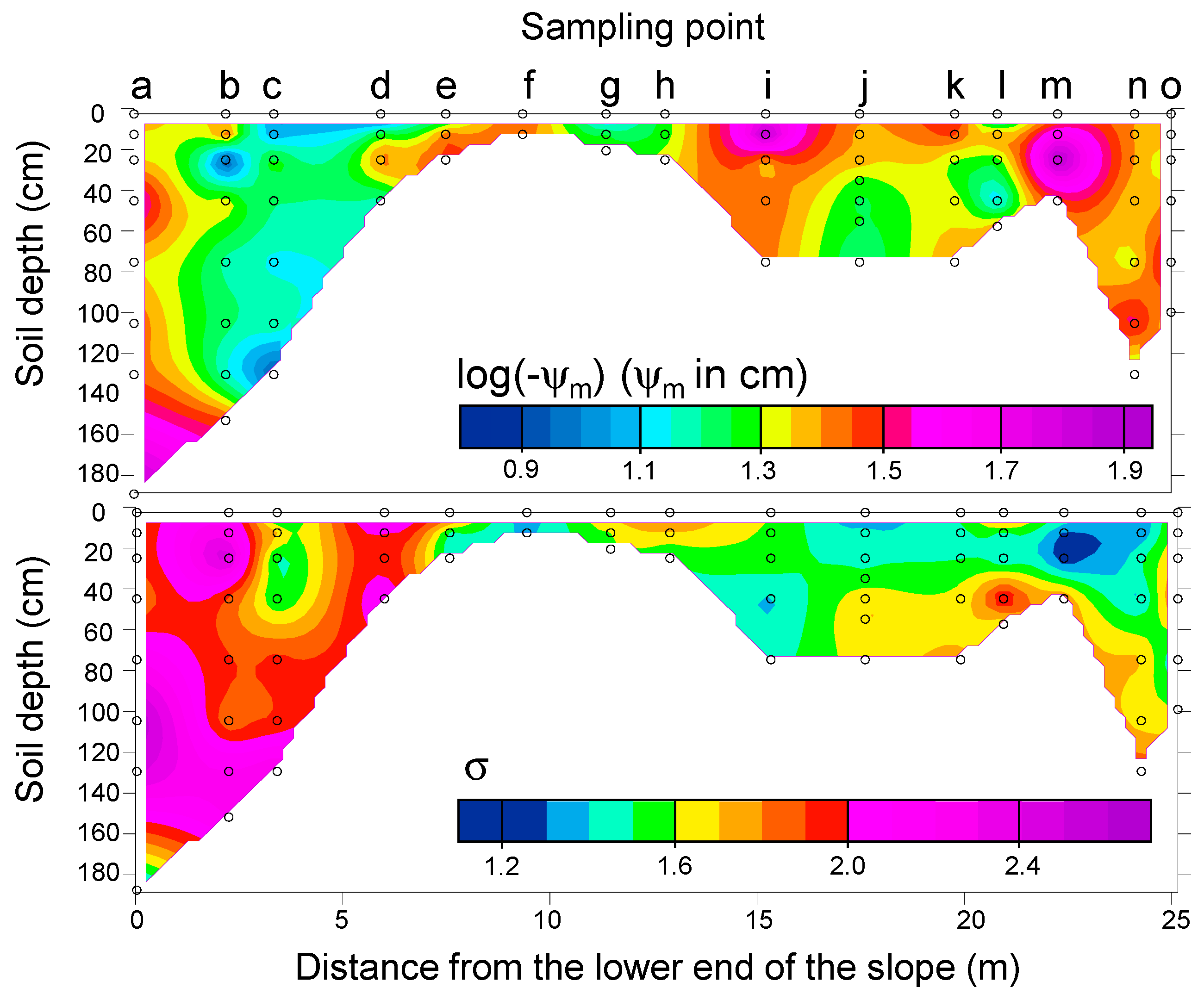
Figure 6.
Relationship between log(-ym) and s and, isolines of the effect of scaling (EOS), expressed as Eq. [12] with EOS = 0, 0.5, 0.6, 0.7, and 0.8. The plots are reference parameters ym and s expressed as Eq. [4] derived from Fitting Approach IF. The lengths of both axes were set such that the standard deviations of both parameters derived from Fitting Approach IF were the same lengths on the panel. n represents the sample size.
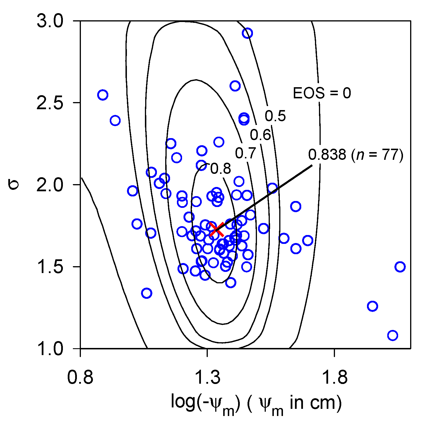
Figure 7.
Cumulative relative frequency distribution of the effect of scaling (EOS), derived from random sampling of WRCs by varying the sample size, n, using a Monte Carlo approach. n represents the sample size.
Figure 7.
Cumulative relative frequency distribution of the effect of scaling (EOS), derived from random sampling of WRCs by varying the sample size, n, using a Monte Carlo approach. n represents the sample size.
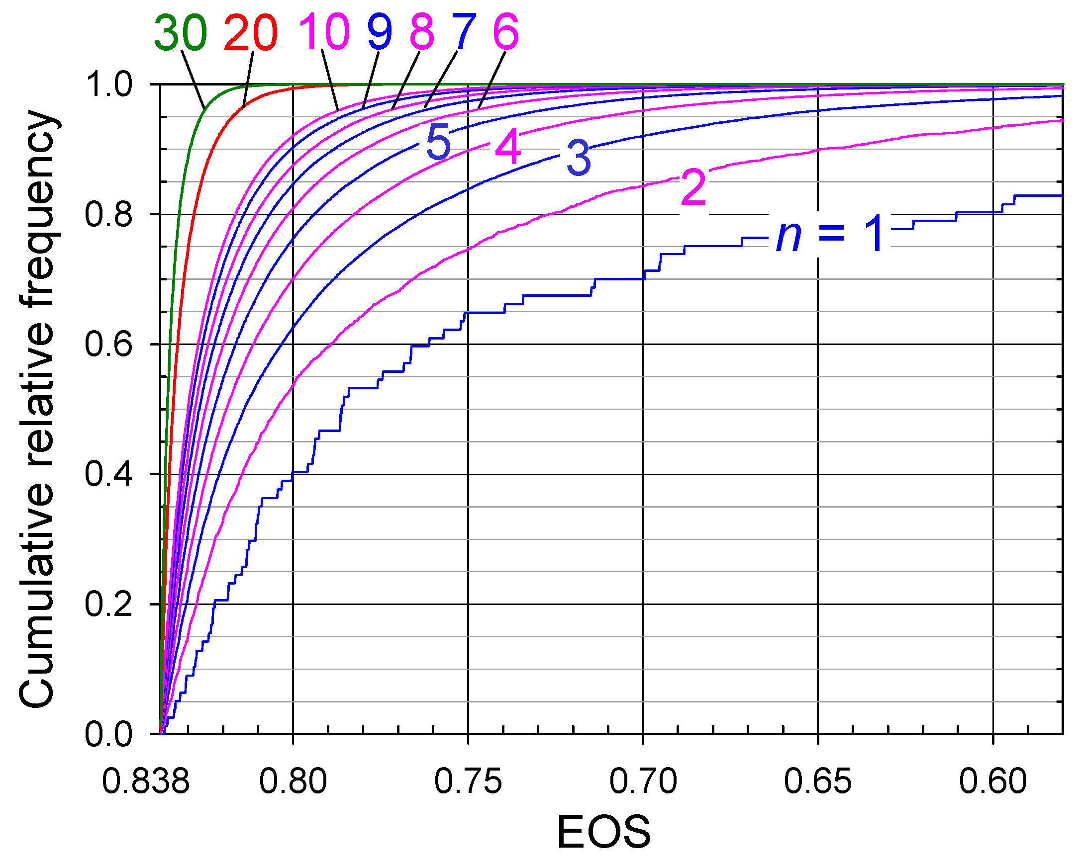
Figure 8.
Relationship between log(-) and derived from water retention curves (WRCs) chosen using random sampling of WRCs by varying the sample size, n, using a Monte Carlo approach for sample size of (a) 3, (b) 7, (c) 8, (d) 20, and (e) 30. The colors on each grid of log(-) and are proportional to the relative frequency of the plot. Isolines indicate effect of scaling (EOS), expressed using Eq. [12] with EOS = 0, 0.5, 0.6, 0.7, and 0.8. The n represents the sample size.
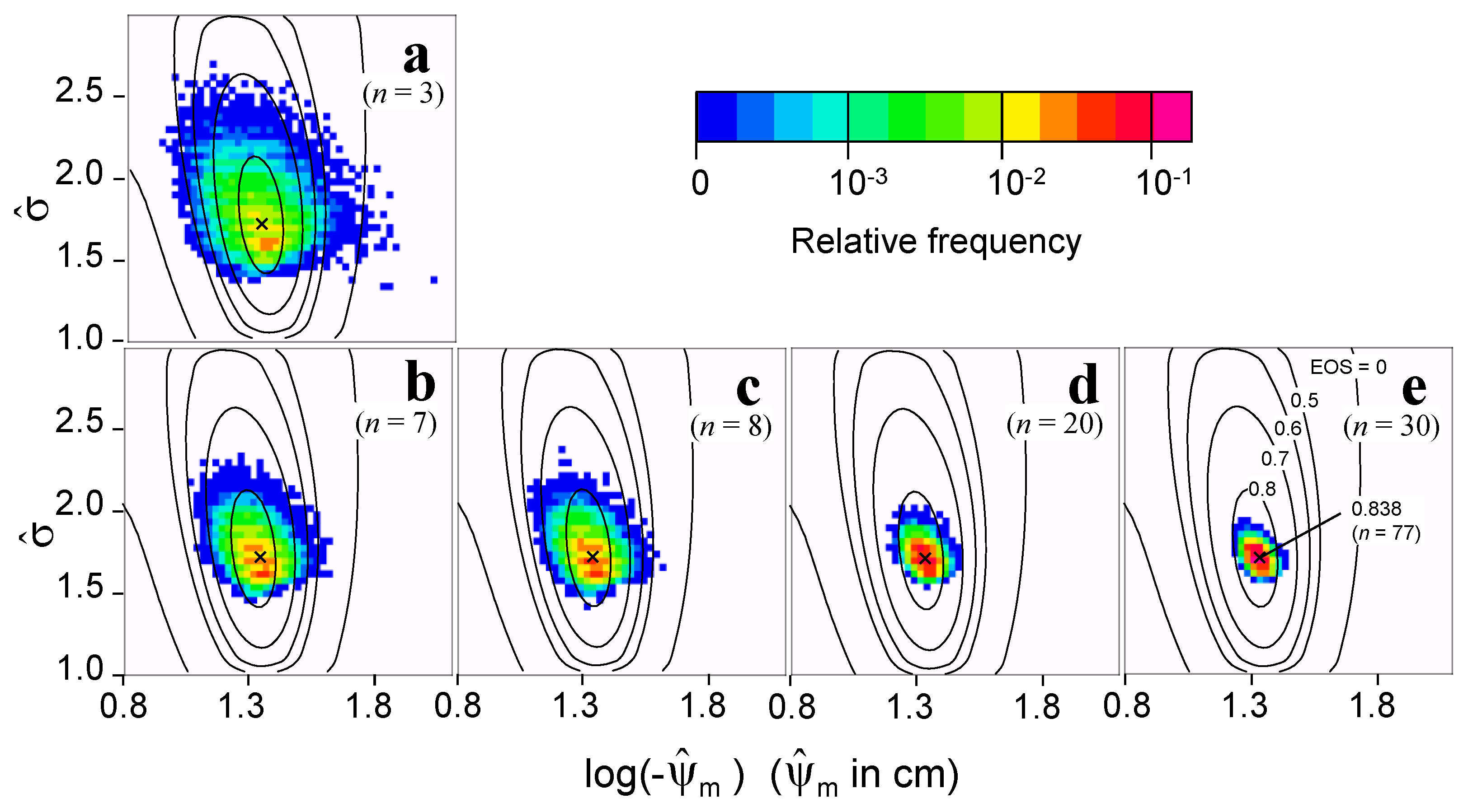
Figure 9.
Relationship between sample size and the effect of scaling (EOS) derived from random sampling of WRCs by varying the sample size, n, using a Monte Carlo approach.
Figure 9.
Relationship between sample size and the effect of scaling (EOS) derived from random sampling of WRCs by varying the sample size, n, using a Monte Carlo approach.
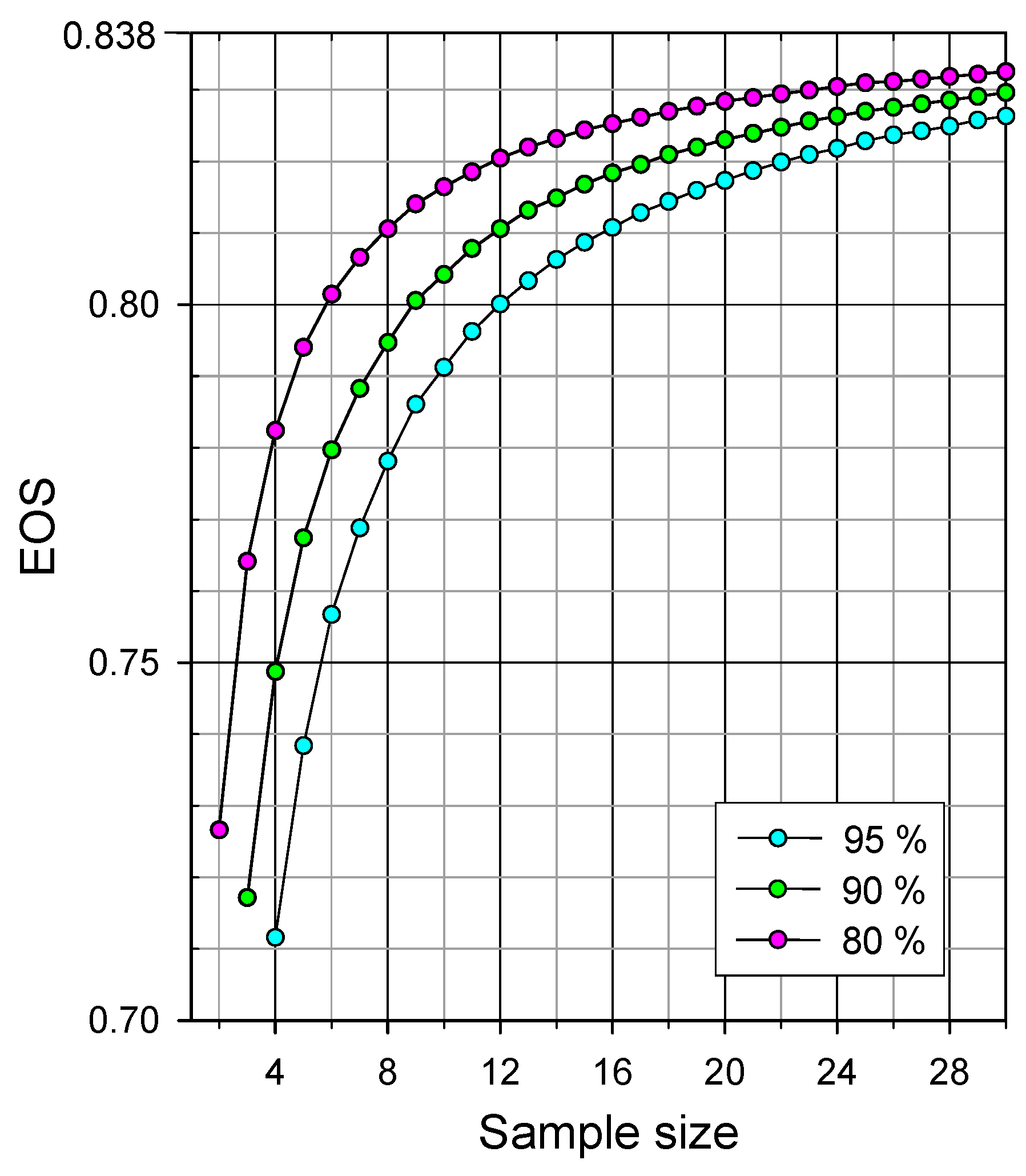
Figure 10.
Schematic representation of the strata used by stratified sampling (a) Schemes 1, (b) 2, and, (c) 3. The blue line is fixed and red lines vary according to the sample size (n).
Figure 10.
Schematic representation of the strata used by stratified sampling (a) Schemes 1, (b) 2, and, (c) 3. The blue line is fixed and red lines vary according to the sample size (n).
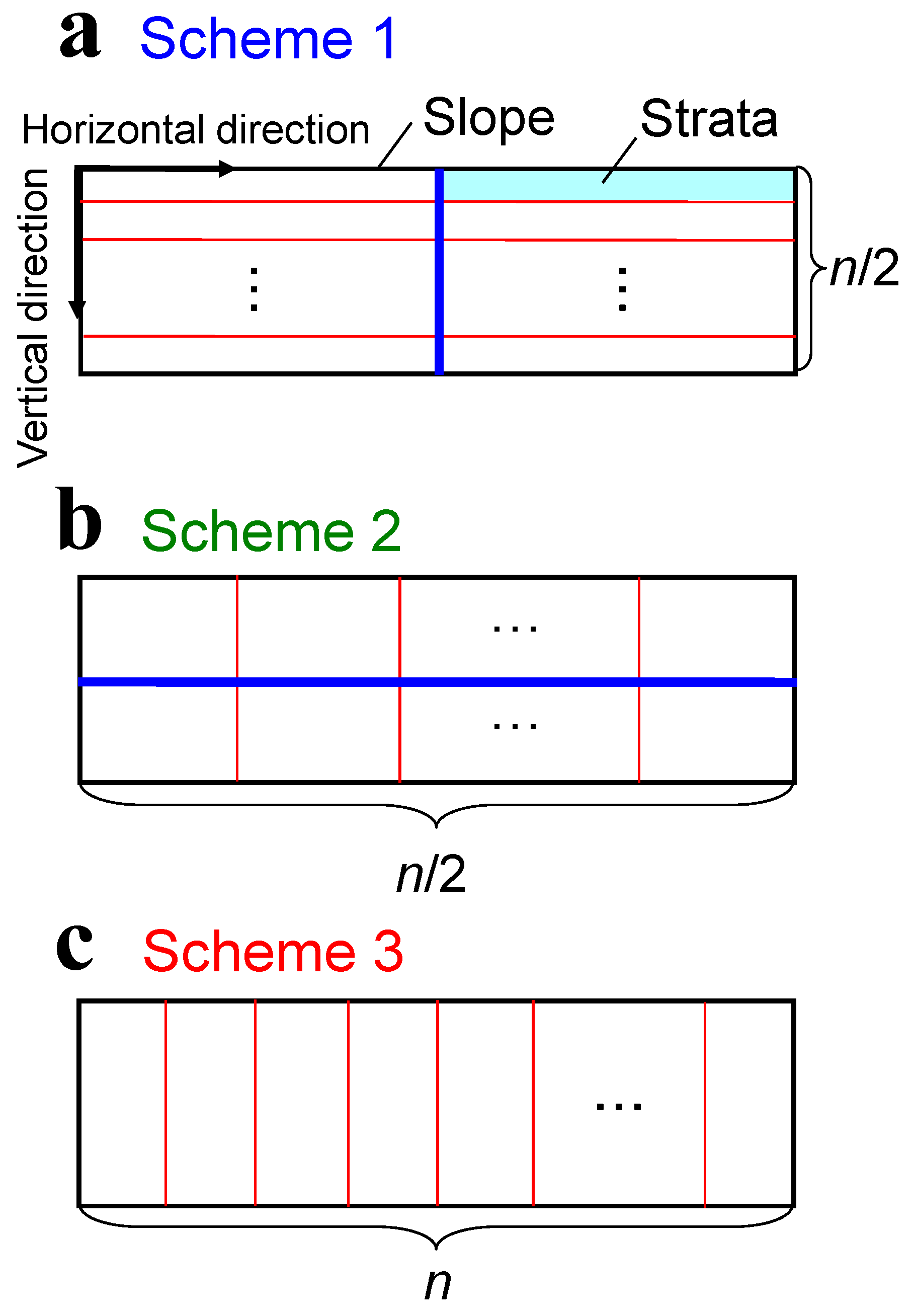
Figure 11.
Cumulative relative frequency of the effect of scaling (EOS) derived from random and stratified sampling of WRCs by varying the sample size, n, using a Monte Carlo approach. The n represents the sample size.
Figure 11.
Cumulative relative frequency of the effect of scaling (EOS) derived from random and stratified sampling of WRCs by varying the sample size, n, using a Monte Carlo approach. The n represents the sample size.
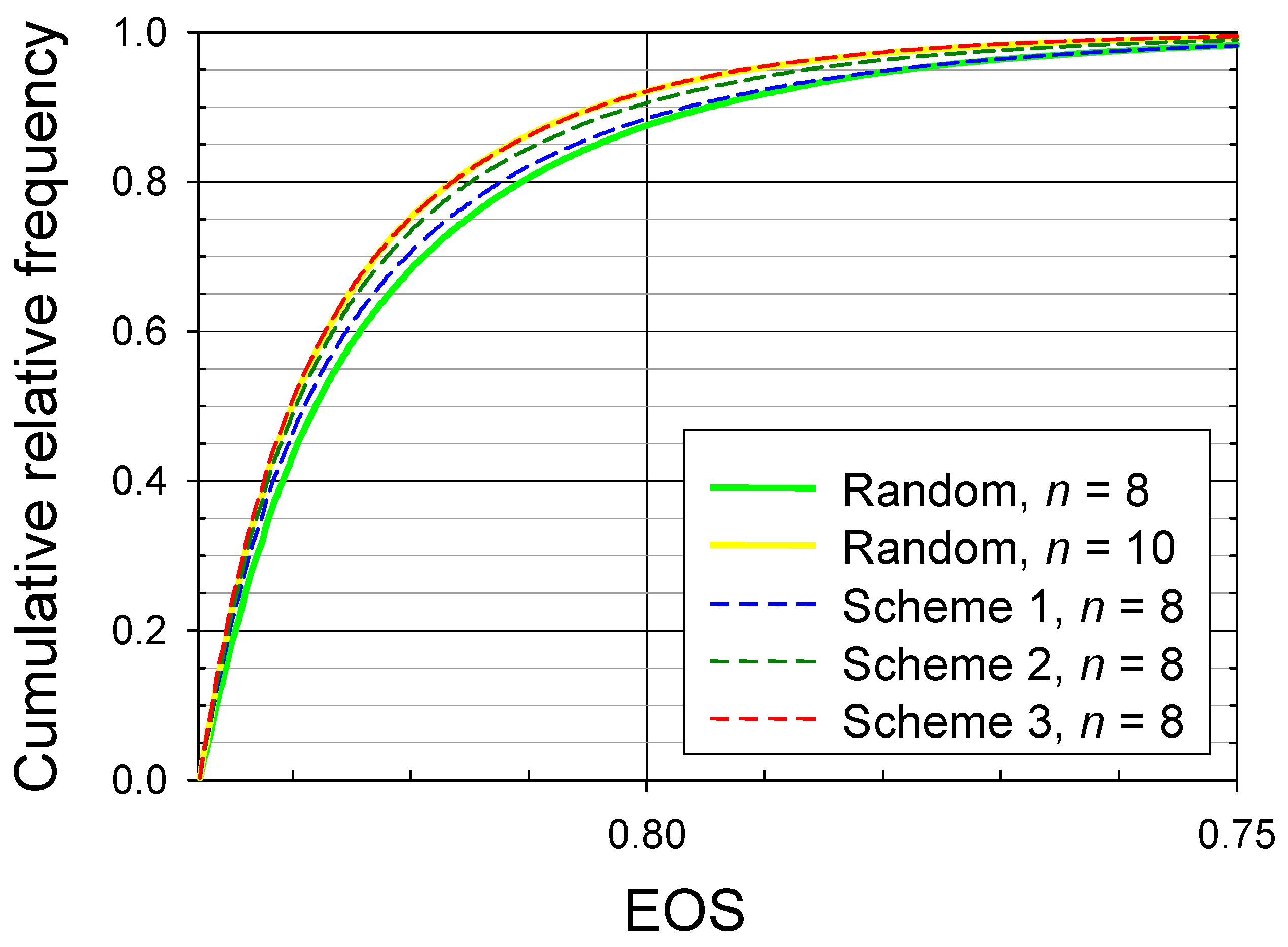
Figure 12.
Semivariograms in the slope and vertical directions for log(-ym) and s. Straight vertical lines indicate the variance of all samples.
Figure 12.
Semivariograms in the slope and vertical directions for log(-ym) and s. Straight vertical lines indicate the variance of all samples.
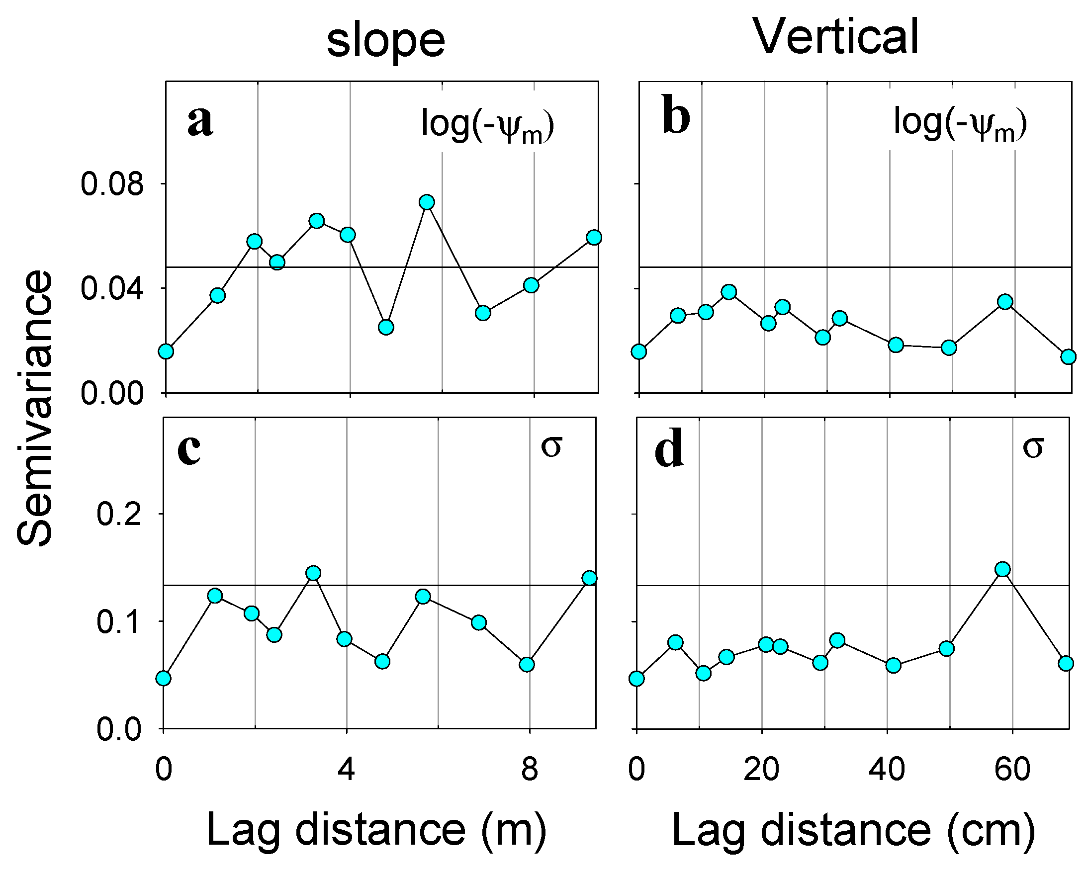

Table 1.
Reference parameters and residual sum of square (RSS), coefficient of determination (R2), and effect of scaling (EOS), for Fitting Approaches IF and UF, and scaling method proposed by Hayashi (2009) using the overall 77 water retention curves (WRCs).
Table 1.
Reference parameters and residual sum of square (RSS), coefficient of determination (R2), and effect of scaling (EOS), for Fitting Approaches IF and UF, and scaling method proposed by Hayashi (2009) using the overall 77 water retention curves (WRCs).
 |
Disclaimer/Publisher’s Note: The statements, opinions and data contained in all publications are solely those of the individual author(s) and contributor(s) and not of MDPI and/or the editor(s). MDPI and/or the editor(s) disclaim responsibility for any injury to people or property resulting from any ideas, methods, instructions or products referred to in the content. |
© 2025 by the authors. Licensee MDPI, Basel, Switzerland. This article is an open access article distributed under the terms and conditions of the Creative Commons Attribution (CC BY) license (http://creativecommons.org/licenses/by/4.0/).
Copyright: This open access article is published under a Creative Commons CC BY 4.0 license, which permit the free download, distribution, and reuse, provided that the author and preprint are cited in any reuse.


