Submitted:
20 November 2025
Posted:
21 November 2025
You are already at the latest version
Abstract
This paper introduces Axiomatic System Dynamics (ASD), a novel, formally self-consistent framework for describing the evolutionary processes of diverse complex systems. ASD is founded on three fundamental axioms which establish a unified, action-driven causal architecture. By utilizing the formal syntax of "State-Action-State Increment," ASD reduces distinct phenomena to Generalized Constitutive Relations that possess a unified structure. This formalization creates a critical bridge between observed phenomena and their mathematical expressions, directly addressing the challenge of incommensurability by providing a common semantic language for models across scientific domains. The framework's efficacy is demonstrated through three progressively complex applications. The analysis of Newtonian Mechanics re-interprets inertia as an Internal Action. The study of material constitutive relations validates the use of the Generalized State Parameter to formally model path dependence and system memory in Non-Markovian systems. Finally, the application to soil consolidation illustrates ASD's power in logically integrating multi-scale, multi-mechanism coupled processes. ASD provides a powerful conceptual tool for advancing the goal of scientific methodological unification.
Keywords:
axiomatic system dynamics (ASD)
; general systems theory
; system dynamics
; complex systems
; state-space
; multiscale modeling
1. Introduction
1.1. The Challenge to Reductionism in Complex Systems
Scientific inquiry has long relied on a two-path strategy: reductionism, which decomposes complex objects into fundamental units to induce universal laws (e.g., Newtonian mechanics); deduction, which uses these laws to reconstruct the behavior of complex systems. This "decompose-and-reconstruct" method has been the cornerstone of modern science, exemplified by the successful derivation of macroscopic laws, such as the Ideal Gas Law , from the principles of statistical mechanics applied to microscopic particle motion.
However, this strategy faces significant limitations in disciplines focused on complex, multi-scale systems that resist simple reduction, such as geomechanics, biology, and social sciences. In soil mechanics, for instance, the macroscopic behavior of a soil element (e.g., constitutive relations, consolidation) cannot be deductively derived from the fundamental laws governing its microscopic components (particles and pore water). This complexity, often rooted in multi-scale structure and stochasticity, necessitates an alternative approach.
1.2. The Problem of Incommensurability
Faced with irreducible complexity, researchers turn to phenomenological modeling, treating the complex object (e.g., a soil element, an ecosystem) as a holistic unit and establishing empirical laws based on observation. While pragmatically effective, this approach leads to a critical fragmentation of knowledge and a pervasive dilemma: incommensurability.
For a complex problem like soil consolidation (Guerriero and Mazzoli, 2021; Holtz et al., 1981; Terzaghi et al., 1996), which involves multiple and mutually coupled mechanisms (external loading, seepage, and creep), the attempt to integrate phenomenological models from specialized sub-fields consistently leads to significant conceptual confusion and physical inconsistency. This integration fails due to the incompatibility rooted in disciplinary specialization, which manifests in three ways:
- 1)
- Semantic Incompatibility: Across sub-fields, the scale of the study object, the primary variables of interest, and the mechanisms that induce change often diverge. Furthermore, inconsistent terminology prevents the semantic alignment necessary for interdisciplinary synthesis.
- 2)
- Logical Disconnect: The causal relationships between different physical mechanisms are not systematically characterized, breaking the chain of inference.
- 3)
- Formal Rigidity: Existing mathematical models are often valid only under specific boundary conditions and lack the formal flexibility to be seamlessly coupled.
Ultimately, this incompatibility prevents the creation of a unified logical platform to describe system evolution across different scales and domains.
1.3. The Gap in Existing Systems Science
The quest for a unified platform gave rise to the Systems Science movement. However, existing theories have failed to resolve the problem of formal incommensurability:
General Systems Theory (GST) (Rousseau, 2015; Von Bertalanffy, 1968): GST's initial goal was to establish a universal, trans-disciplinary language to study common laws across all systems. While establishing the "system" concept and highlighting cross-disciplinary isomorphisms, GST remains largely philosophical and qualitative, lacking the rigorous formal syntax needed for hard sciences.
Cybernetics and Control Theory (Ashby, 1956; Chen, 1984): These disciplines established the rigorous state-space framework for dynamic systems. However, they presuppose that the system's state variables and dynamic equations are already known (identified systems), offering no methodology for discovering the state space of an unknown, complex system (wait-to-be-identified systems).
System Dynamics (SD) (Richardson, 2011; Sterman, 2018) and Complexity Science (Kauffman, 1992; Thurner, 2018): While offering tools for feedback and emergence, SD lacks axiomatic rigor, and Complexity Science provides disparate mathematical tools without a unified formal framework.
Later developments including Soft and Critical Systems Methodology (Cabrera et al., 2023; Checkland and Poulter, 2020; Jackson, 2016, 2019; Midgley, 2000; Rousseau, 2017; Suh, 1998) largely abandoned the pursuit of a universal, formal language. Consequently, a structural gap remains: no existing theory simultaneously possesses the philosophical universality of GST and the mathematical rigor of Control Theory while being applicable to the identification of unknown systems.
1.4. Introducing Axiomatic System Dynamics (ASD)
To bridge the crucial structural gap left by existing systems theories, this paper introduces Axiomatic System Dynamics (ASD). ASD is a rigorous, content-free meta-theory constructed from three fundamental axioms. It does not aim to replace existing physical laws, but rather to establish a universal syntax—centered on the primitives of State, Action, and State Increment—that acts as a semantic bridge for specialized disciplines.
By structuring the causal logic of system evolution, ASD provides a logically consistent platform for integrating incommensurable models. This is achieved by establishing the research path as "Conceptual Model first, Mathematical Model second," which forces semantic alignment before mathematical implementation. This framework may serve as a critical step toward realizing the founder's ambition of GST.
2. Fundamental Axioms
The First Axiom of State Change (Axiom 1): Action is the sole factor that causes a change in the system's state. The system's state at time and the action exerted on the system during the time interval uniquely determine the state increment during that interval.
The Second Axiom of State Change (Axiom 2): The system's state at time uniquely determines the internal action exerted on the system during the time interval .
The External Action Induction Principle (B-A Principle): If a system's state at time is , the external action received during the time interval is , and the resulting state increment is ; and if the system's state at time is also , the external action received during the time interval is zero, and the resulting state increment is . Then, the state increment of the system due solely to the external action during is defined as the difference .
3. Fundamental Concepts
3.1. Primary Concepts
System. The system is the object of study. It encompasses the physical parts of the object and a portion of the influence of the environment upon those physical parts.
State. The state represents "what the system is like." It is the decisive basis for determining the system's response (state increment) under any action. The state is an ontological concept; the system's state exists and is unique at any given time . We denote the state using the symbol .
Action. Action is the sole factor that changes the system's state, and it is also an ontological concept. Action is always defined over a time interval ; considering the action at a single moment is meaningless.
Parameter. A parameter is a measurable attribute of the system, representing the quantitative feature of the state. Compared to the state, the parameter is an epistemological concept. The parameters of the system at any time are entirely determined by the state at time . If two systems have the same state at the same time, all their corresponding parameters are identical; however, the converse is not necessarily true, as any set of measurable parameters may not completely describe the system's ontological state.
Characteristic Time Scale. The characteristic time scale is the time interval used in the fundamental axioms. It represents the temporal scale at which we observe and comprehend the system's behavior. The system's dynamic characteristics may vary significantly under different characteristic time scales, necessitating its determination in the study.
3.2. Secondary Concepts
Target Parameter. The target parameters are the system parameters of most concern in the study. In specific research, we are not interested in the ontological state; the full set of the system's characteristics is usually impossible, and unnecessary, to fully understand. We are concerned only with a portion of the system's characteristics, and the target parameters are the concentrated manifestation of this portion. The objective of the research is to study the changes in the system's target parameters during the state change process. For example, when studying the motion of a particle, the particle's position is a target parameter, and its shape and spatial orientation may sometimes be included, but the particle's color and price are typically not.
Internal Action and External Action. Internal action is the action exerted by the system on itself, and external action is the action exerted on the system by the external environment. The total action received by the system is a function of these two, i.e., . According to Axiom 2, the system is unconditionally subject to its internal action. The internal action does not necessarily originate solely from the physical parts of the object of study; it may include some environmental influences upon it. The demarcation between internal and external actions is the result of defining the system boundary. This division is related not only to the material properties of the object of study but also to the specific research purpose, and it must strictly adhere to Axiom 2. Those environmental influences classified as internal action may change as the system's state changes
Generalized Constitutive Relation. The generalized constitutive relation is any functional relationship that satisfies Equation (1) and possesses the expression form of "State-Action-State Increment." The generalized constitutive relation is used to express the ontological system dynamics conceptual model. It requires the quantification of the state and the action before a specific mathematical model can be obtained. While expressed mathematically as the function , the notation from Equation (1) is used to emphasize the causal relationship described by Axiom 1 and to distinguish it from other simultaneous functional relationships, a convenience that is more pronounced when multiple generalized constitutive relations are involved.
Coupling and Decoupling of Actions. The total action received by the system can be decomposed according to underlying mechanisms into several types of sub-actions . In this case, the total action is the coupling of these sub-actions, i.e., . If the system's response under the coupled effect of these sub-actions can be (approximately) regarded as the linear superposition of the responses under each sub-action acting alone, then these sub-actions are said to be decoupled. Specifically, assuming the system's response under the coupled action is:
then these sub-actions are decoupled if:
By the B-A Principle, the decoupling of the system's total internal action and total external action is a logical necessity.
State Creep Process. The state creep process is the process of state change (including the process of no change) that occurs when the system is subjected to no external action, operating solely under its internal action. It represents the system's pure spontaneous evolution. The state creep process is determined solely by the system's initial State, a property derived as a logical consequence of Axioms 1 and 2.
3.3. Tertiary Concepts
State Space and State Path. To provide an abstract geometric representation of the system's state, the state can be viewed as a point in a state space. The process of state change can be viewed as a parametric curve in the state space with time as the parameter; this curve is called the system's state path.
External Action Space and External Action Path. If there exists a function with time as the independent variable, such that the external action exerted on the system during any time interval is completely determined by the function segment , i.e., there exists a functional relationship:
Then, the function is called the external action path of the external action , and the image space of function is called the external action space. If the external action received by the system can be reduced to certain system parameters, or to the active alteration of these parameters, then the space where these parameters reside can serve as the external action space, and the function of these parameters with respect to time can serve as the external action path . In this case, within the generalized constitutive relation, the external action during any interval can be directly equivalent to the function segment , i.e.:
This allows the external action to be quantified.
State Parameter. A state parameter is a parameter that can serve as an equivalent substitute for the system's state in specific research. The state parameter should determine or contain the target parameters and serve as the decisive basis for the evolution of the state parameter itself when the system undergoes state change under internal and external actions. A system's state parameter does not necessarily exist. The system's state is ontological and cannot necessarily be characterized by a finite number of observable parameters; the existence of state parameters, or the describability of the system state, is epistemological. The existence of state parameters, and which system parameters constitute them if they do exist, is usually closely related to the target parameters, the system's initial state, and the potential external actions. The state parameter is a method for describing Markovian systems.
External Action History and Generalized State Parameter. If the system's initial state at a certain time is known, and the external action has an external action path , then according to Axioms 1 and 2, the system's state at any time is a functional of the initial state and the function segment , i.e.:
In this case, the function segment is called the system's external action history (at time ). The determination of the system state by the external action history possesses logical redundancy: for a given initial state, if the external action history is the same, the system's current state is the same; however, the converse is not necessarily true, because different external action histories may lead to the same current state.
In scientific research, one usually observes which features of the external action history (such as endpoint function values, integral averages, etc.) predominantly determine the changes in the system's target parameters. Combining these features of the external action history with some other system parameters to form a composite parameter serving as an equivalent substitute for the system state , this composite parameter is called the generalized state parameter. Functionally, like a state parameter, the generalized state parameter should determine or contain the target parameters and serve as the decisive basis for the evolution of the generalized state parameter itself when the system undergoes state change under internal and external actions. Strictly speaking, a generalized state parameter is not necessarily a general parameter, because it is not necessarily determined solely by the state at time , but possesses historicity. The generalized state parameter is a method for describing Non-Markovian systems.
4. Illustrative Applications
The following section presents three representative examples to demonstrate the mapping relationship between ASD conceptual models and specific mathematical models. The discussion will focus on the structural mapping rather than the historical development or epistemological origins of these models.
4.1. Newtonian Particle Mechanics
Consider the motion of a particle under external forces within an inertial reference frame. The system is the particle itself. The target parameter is the particle's spatial position vector . The internal action represents the effect of the particle's inertia. The external action represents the effect of the net external force acting on the particle. The ASD conceptual model for Newtonian particle mechanics is shown below:
To transform the conceptual model into a mathematical model, the system's state , internal action , and external action must be quantified. According to Axiom 2, the quantification of the internal action is achieved indirectly through the quantification of the state .
In Newtonian particle mechanics, the state is quantified via state parameters. The state parameters are the particle's position , velocity , and mass ; thus, the state is defined as . Note that the state parameters encompass the target parameter, and mass is included because it is strictly necessary to determine the state increment (specifically the velocity change) induced by the external action.
The external action is quantified via an external action path. The external action path is the function of the net external force over time , therefore. According to Equation (7), the external action within any time interval is:
When the characteristic time scale approaches zero, the external action is determined solely by the value at the left endpoint of the function segment —namely, the value of the net external force at time . Consequently, Equation (12) simplifies to:
The mathematical model derived from the ASD conceptual model is as follows:
Equations (14) and (15) correspond to Newton's First Law and Newton's Second Law, respectively. By observing the iterative relationship of velocity in Equation (15), one can derive the standard expression of Newton's Second Law: .
The conceptual model of Newtonian particle mechanics represents the simplest form of an ASD conceptual model, containing exactly one internal action and one external action. The particle's uniform linear motion constitutes the system's state creep process. Here, inertia is conceptualized as an internal action. Uniform linear motion is thus interpreted as a continuous state change generated by this internal action, rather than the unconditional persistence described in traditional Newtonian mechanics. Admittedly, a system's state change in the absence of external action could be viewed as a spontaneous evolution free from any action. However, Axiom 1 emphasizes that action is the sole factor changing the system's state; this stipulation provides greater logical and formal uniformity when explaining the causality of state changes.
From an epistemological perspective, experimental observation can only directly yield the generalized constitutive relation for the internal action (Equation 14) and the generalized constitutive relation for the coupled internal and external actions (Equation 16). The generalized constitutive relation for the external action (Equation 15) must be obtained indirectly via the B-A Principle (the logic of controlled experiments).
4.2. The Stress-Strain Constitutive Relation of Materials
As shown in Figure 1, consider a material element within a triaxial testing apparatus. In this test, we can measure the confining stress and axial stress , as well as the radial strain and axial strain . Assume that at time , the element is in an initial state corresponding to a stress , and that the initial state is identical across repeated experiments. By observing the strain paths of the element under various manually controlled stress paths , we aim to derive its Stress-Strain Constitutive Relation (Dill, 2006; Lai et al., 2009). Secondary effects such as heat conduction are neglected.
The system is the material element. The target parameters are the stress and strain of the element. The internal action represents the action determined solely by the material's intrinsic properties, independent of the changes in stress , relating to the material's creep or rheological characteristics. The external action represents the action on the element caused by changes in stress .
The ASD conceptual model for the material element is structurally identical to that of Newtonian particle mechanics (Equations 9-11). However, compared to the previous example, quantifying the state and external action for a material element is more difficult due to the complexity of real material microstructures.
4.2.1. Path Dependence and Non-Markovian Nature
The stress-strain relationship of a material element typically exhibits path dependence. That is, the state of the element at time depends not only on its stress and strain at time but also on its loading history (stress history) . Furthermore, for two states and , even if their stress , strain , and other microscopic parameters (e.g., pore size distribution, particle orientation frequency, fractal dimension in porous media) are identical, there is no guarantee that the states are truly identical. Even if their subsequent stress paths are identical, their strain paths may diverge significantly. Therefore, a material element is typically a Non-Markovian system, making it difficult to identify a definitive set of state parameters.
The external action is quantified via an external action path , specifically the stress path , therefore . According to Equation (7), the external action in any time interval is:
Due to the element's path dependence and rate dependence, starting from a state at time , the strain increment during depends not only on the stress increment contained within the stress variation , but potentially also on the shape of the curve in stress space and other properties. This prevents us from simplifying Equation (17) directly to without considering specific material properties.
4.2.2. Generalized State Parameters and Mathematical Modeling
To determine the state of the material element, the approach in mechanics essentially employs generalized state parameters. Based on Equation (8), the stress history up to any moment determines the state at that moment, which in turn determines the strain at time . Thus, the simplest approach is to select the stress history itself as the generalized state parameter:
In our stress-controlled experiments, the stress history is fully determined at any time , so the conceptual model (Equations 9-11) is effectively transformed into mathematical expressions. Since the generalized state parameter does not directly contain strain , we must determine the specific functional relationship of strain with respect to stress history:
This yields the mathematical model for the material's stress-strain constitutive relation. The expressions for the strain increments contained in and are, respectively:
Simply put, the strain increment under the internal action represents the creep deformation unrelated to stress change, generated during the interval when the stress remains constant at value . This represents the system's baseline response in the absence of external action.
Conversely, the strain increment under the external action represents the difference between the actual strain increment produced when the stress changes as during and . This represents the difference between the actual response under coupled internal and external actions and the baseline response. From an epistemological perspective, can only be obtained indirectly through the B-A Principle or controlled experiments.
Directly using the entire stress history as generalized state parameter (Equation 18) makes the functional relationship in Equation (19) extremely complex, as experiments cannot exhaust all possible stress histories. Therefore, mechanics assumes that partial features of the stress history determine the current state , using these features as the generalized state parameter. We illustrate this with Elastic and Elasto-Plastic models.
4.2.3. Rate-Independent Models (Elastic and Elasto-Plastic)
Both Elastic and Elasto-Plastic models are rate-independent models. The assumptions of rate-independent models can be summarized in two points:
- The geometric curve shape of the stress history in stress space (as illustrated by curve AB in Figure 2) uniquely determines the element's state at time , regardless of the rate at which the loading is performed. In the context of rate-independent models, where no confusion arises, the curve shape is also referred to as the stress history.
- Starting from a given state at time , the state increment during the interval depends solely on the curve shape of the stress variation in stress space. Furthermore, as the characteristic time scale approaches zero,depends solely on the vector formed by the two endpoints of this curve—namely, the stress increment . Geometrically, the stress history at time "adds" this increment to yield the stress history at time .
These assumptions introduce two simplification effects for the analysis. First, the state increment produced by the internal action in Equation (9) is always zero. This allows the internal action to be directly ignored during analysis, resulting in and . This occurs because the element's response under internal action is the response corresponding to a zero stress increment , so the stress history at time is effectively the same as the stress history at time in a geometric sense (i.e., the path has not changed).
Second, the stress history can be chosen as the generalized state parameter, defining the state at any time as:
Consequently, Equation (19) simplifies to:
And Equation (17) simplifies to:
The rate-independent model can be figuratively described as a geometry that studies the strain corresponding to different stress histories in the stress space.
Elastic model is the simplest rate-independent model. It further assumes that the endpoint of the stress history (point B in Figure 2), which is the current stress , completely determines the current State . The stress can be chosen as the generalized state parameter, simplifying Equation (22) to:
At this point, the generalized state parameter is composed entirely of general parameter, and it degrades into the system's state parameter. The historicity has been eliminated, and the element becomes a Markovian system. Equation (23) simplifies to:
Strain is purely a function of stress , which fully reflects the characteristics of elasticity.
The Elasto-Plastic model builds upon the Elastic model by additionally considering plastic strain. The element's total strain is conceptually separated into elastic strain and plastic strain :
Where the elastic strain is calculated using the Elastic model:
To determine the plastic strain , it is necessary to define internal variable , which are typically used to characterize the material's microstructural state. Two constitutive functions, the yield function and the plastic potential function , which are functions of the internal variable and stress , are then defined. At any time , the element's stress , the constitutive functions and , and the stress increment during the interval collectively determine the plastic strain increment and the internal variable increment (which may be zero) during the interval. This determination involves concepts such as the Loading Condition, Plastic Flow Rule, and Consistency Condition (Hill, 1998; Khan, 1995). Logically, given the initial internal variable and plastic strain of the initial state , the internal variable and plastic strain corresponding to any stress history can be uniquely determined through a recursive procedure, therefore:
Furthermore, if the internal variable , plastic strain , and stress at time are known, their increments during the interval can be determined by the stress increment .
From a theoretical standpoint, the internal variable , as artificially defined variables, do not have a clear physical meaning and cannot be obtained by measuring the state at time . Plastic strain is defined as the residual strain after the stress is unloaded from the state back to the initial value . For an actual material element, the plastic strain obtained via different unloading stress paths may not be identical. This indicates that, without relying on additional assumptions, plastic strain is not necessarily a well-defined system parameter.
Therefore, in the Elasto-Plastic model, the internal variable and plastic strain are not general system parameters, but rather specific features of the stress history . The Elasto-Plastic model essentially uses the triplet , , as the generalized state parameter, defining the state at any time as:
The elastic strain is determined by the stress , and the plastic strain is directly included in the generalized state parameter, determined through the recursive procedure.
4.2.4. Discussion on Action Partitioning
The above study of the material element's stress-strain constitutive relation fully demonstrates how to establish the corresponding mathematical model based on the simplest ASD conceptual model when facing Non-Markovian systems. Simultaneously, it explicitly clarifies the introduction and application method of the generalized state parameter.
Comparing the particle example with the material element example, a difference in the partition of internal and external actions can be observed.
For the material element, its response under internal action represents the response when the stress remains constant at during the interval , rather than the response when it is completely unloaded (). During this period, the stress received by the element originates from the physical exterior, for example, from the fluid in the triaxial test chamber or the axial loading ram. It is an environmental action, but in this context, this stress is considered part of the internal action . The information determining this part of the internal action is the stress at time ; it is a parameter of the system at time and is contained within the state at time . This adheres to the requirement of Axiom 2.
In contrast, the element's response under external action is the difference between the actual response and , generated when the stress changes relative to during the interval . represents the net effect caused by this stress change and is the result of applying the B-A Principle.
Defining the element's response under internal action as the response when stress is held constant at , rather than the response when is zero, is determined by the research objective. In real-world scenarios, a material element is always situated in a specific environment and under a certain initial stress state. We need to study its response under additional loading, not the response of an initially stress-free element to loading. The situation of a completely stress-free element is highly specialized. This is also why the material's creep is defined as the behavior under constant stress.
This example highlights that: the internal action received by the system may include a portion of environmental action, and the partition of internal and external actions is related to the research objective, but must always comply with Axiom 2.
4.3. One-Dimensional Consolidation of Saturated Soil
In soil mechanics (Guerriero and Mazzoli, 2021; Holtz et al., 1981; Terzaghi et al., 1996), the consolidation of saturated soil is the process by which internal pore water gradually drains out under external load, usually accompanied by the gradual dissipation of pore water pressure and the continuous increase in effective stress. Terzaghi's one-dimensional consolidation theory (Terzaghi, 1925, 1943) is the most classic consolidation theory, which has been greatly developed over the past 100 years (Guerriero, 2022; Radhika et al., 2020).
As shown in Figure 3, we consider a one-dimensional consolidation problem of a saturated soil sample under an initially () applied additional external load . The system is the soil sample. The soil sample is composed of countless soil elements; the soil element is the Subsystem. The state of the soil element is denoted by . The state of the soil sample is determined by the states of all soil elements and can therefore be represented as a state distribution . The target parameters for the soil element are the total stress , effective stress , pore water pressure , and void ratio ; for the soil sample, they are the spatial distributions of these parameters , , , . The Principle of Effective Stress:
is the fundamental principle of soil mechanics. Small strain assumption is adopted in the analysis.
4.3.1. Soil Element Subsystem
For the soil element, it is subjected to three approximately decouplable actions: external load action , seepage action , and creep action .
Among these, the creep action is the internal action of the soil element, representing the action determined solely by the soil's intrinsic properties, independent of total stress change and seepage, and related to the soil's creep or rheological characteristics. The external load action and seepage action are the external actions of the soil element. The external load action represents the action generated by the change in total stress , independent of seepage. The seepage action represents the action generated by the volume change of the element due to seepage, independent of total stress change. Therefore, the ASD conceptual model for the soil element is:
The generalized constitutive relations for the external load action , seepage action , and creep action are the conceptual abstractions of the soil's stress-strain constitutive relation; they describe three independent physical mechanisms.
External load action is quantified via an external action path. Since the change in total stress originates from the additional external load (where ), the external action path is defined as the external load , i.e., . According to Equation (7), the external load action during any interval is:
Seepage action can be quantified by the change in void ratio caused by seepage:
Seepage action is the only action that can cause a change in the void ratio ; thus, . According to Axiom 2, the quantification of creep action is completed indirectly through the quantification of the state .
4.3.2. Soil Sample System
For the soil sample, it is similarly subjected to the external load action , seepage action , and creep action , which have the same physical meaning. Its ASD conceptual model is:
In any time interval , the soil sample's response under the external load action is equal to the spatial distribution of the responses of all soil elements within it under their respective external load action . The same applies to seepage action and creep action . For the soil sample, the quantification of the external load action is the same as Equation (36). Therefore, if we obtain the mathematical expressions for the generalized constitutive relations of the soil element under external load action and creep action , we simultaneously obtain the mathematical expressions of the soil sample under these two actions.
The crucial issue arises with the seepage action of the soil sample. According to Equation (37), the soil sample's seepage action is quantified as . But how do we know the distribution of the void ratio increment during the interval ?
Seepage is the liquid-phase transport process within the soil sample. Its genesis essentially originates from the non-uniform distribution of soil element states , and is predominantly governed by the non-uniform pore water pressure distribution contained within that state distribution. Therefore, as long as the state distribution at time and the soil sample's drainage boundary conditions are determined, the instantaneous seepage velocity distribution within the soil sample can be determined. The non-uniformity of the seepage velocity distribution further leads to a net change in the pore water volume of the soil elements during the interval , thereby determining the void ratio increment distribution .
Therefore, by incorporating the soil sample's drainage boundary conditions into its state , the generalized constitutive relation for the soil sample under seepage action , Equation (39), is decomposed as follows:
Equation (42) indicates that the state distribution at time determines the seepage velocity distribution at time . The specific mathematical expression for this equation is the Permeability Law, such as the Darcy permeability law adopted by Terzaghi:
Where is the permeability coefficient, and is the unit weight of water (a constant). Equation (43) indicates that the seepage velocity distribution at time determines the void ratio increment distribution during the interval . The specific mathematical expression for this equation is the Continuity Condition, which represents the relationship between the net inflow of pore water and the change in the pore volume of the soil element. Under the small strain assumption and assuming incompressible pore water and soil particles, Equation (43) is equivalent to:
Where is the initial void ratio at . Equation (44) is simply the spatial aggregation of the generalized constitutive relations (33) for all soil elements under seepage action .
It is clear from Equations (42) to (44) that the soil sample's response under seepage action is entirely determined by its state . By Axiom 2, the seepage action has become the internal action of the soil sample. For the soil sample system, its internal actions are seepage action and creep action , while its external action is the external load action , which is solely determined by the external load . Therefore, the method of partitioning internal and external actions differs between the soil sample system and the soil element subsystem.
4.3.3. Derivation of Specific Mathematical Models
In summary, the ASD conceptual model for one-dimensional consolidation is shown in Figure 4.
Now, it is only necessary to quantify the state of the soil element using an appropriate method, and based on this, select the mathematical expressions for the soil element's stress-strain constitutive relation (Equations 32–34), the permeability law (Equation 42), and the continuity condition (Equation 43), in order to obtain a specific one-dimensional consolidation mathematical model. We will present three examples below.
First, we choose all the soil element's target parameters as its state parameters. Thus, the state of the soil element is , and the state of the soil sample is .
We begin by considering the seepage action . For the permeability law, we select the Darcy permeability law from Equation (45). For the continuity condition, we select the form from Equation (46) assuming incompressible pore water and soil particles. Note that in Equation (33), always. By the principle of effective stress, we only need to determine the relationship between and to specify this equation. Assuming a linear relationship exists between and , the stress-strain constitutive relation of Equation (33) is:
Where is the coefficient of compressibility. By combining Equations (45) to (47), we obtain the mathematical expression for the generalized constitutive relation (39) of the soil sample under seepage action :
It should be noted that because the soil element state is , without further assumptions, both the coefficient of compressibility and the permeability coefficient in the equation are functions of the state . Additional functional relationships must be determined to obtain the complete expression of Equation (48). For this purpose, Terzaghi further assumed that and are constants and uniform throughout the soil sample. Equation (48) is then simplified to:
Where is the coefficient of consolidation (a constant here). The above equation is the specific mathematical expression for the generalized constitutive relation of the soil sample under seepage action in Terzaghi's consolidation theory.
As the simplest static consolidation theory, Terzaghi's consolidation theory neglects external load action and creep action . In this case, , and Equation (49) is the total state evolution equation. By observing the iterative pattern of the pore water pressure within it, the classic Terzaghi one-dimensional consolidation equation is obtained (Terzaghi, 1925, 1943):
This equation can be solved by combining certain drainage boundary conditions and the initial condition at .
Further consider the external load action . Note that in Equation (32), always. Considering the soil sample in a laterally constrained one-dimensional strain state, and combining this with the already-adopted assumption of incompressible pore water and soil particles, the stress-strain constitutive relation of Equation (32) becomes:
That is, the external load action can only cause equal changes in the soil element's total stress and pore water pressure . The corresponding mathematical expression for the generalized constitutive relation (38) of the soil sample under external load action is:
By combining Equation (52) and (49), we can obtain a class of consolidation theories based on Terzaghi's consolidation theory that additionally consider a varying external load (Baligh and Levadoux, 1978; Wilson and Elgohary, 1974; Ying-chun and Kang-he, 2005). The total state evolution equation is:
By observing the iterative pattern of the pore water pressure within it, the corresponding consolidation equation is obtained (Baligh and Levadoux, 1978; Ying-chun and Kang-he, 2005):
This equation can be solved by combining certain drainage boundary conditions and the initial condition at .
Further consider the creep action . Note that in Equation (34), always. We adopt the Yin-Graham Elastic-Viscoplastic (EVP) model (Yin and Graham, 1994, 1996, 1999; Islam and Gnanendran, 2017), in which the soil element's stress relaxation satisfies an equation of the following form:
Where is the viscoplastic rate of the effective stress. Since it is already a function of the soil element's state , it is a complete expression. Combining this with the principle of effective stress, the stress-strain constitutive relation of Equation (34) is:
That is, creep action can only cause equal and opposite changes in the soil element's effective stress and pore water pressure . The corresponding mathematical expression for the generalized constitutive relation (40) of the soil sample under creep action is:
By combining Equations (57), (52), and (49), we obtain a class of consolidation theories based on Terzaghi's consolidation theory that additionally considers a varying external load and creep characteristics (Yin and Graham, 1996). The total state evolution equation is:
By observing the iterative patterns of the pore water pressure and void ratio within it, the corresponding consolidation equation is obtained (Yin and Graham, 1996):
This equation can be solved by combining certain drainage boundary conditions and the initial condition at . It should be noted that the differential equation for pore water pressure alone is not complete here, because the viscoplastic change rate:
cannot be expressed as a function of alone, but can be expressed as a function of and .
The above example of consolidation research effectively demonstrates how to establish a logically clear ASD conceptual model and subsequently derive the corresponding mathematical models when dealing with multi-scale objects and multiple physical mechanisms. By selecting different specific mathematical models or expressions for the stress-strain constitutive relation (Equations 32–34), the soil's permeability law (Equation 42), and the continuity condition (Equation 43), a wider variety of consolidation models can be obtained. The prerequisite is that the quantification method of the soil element state must be uniform, and all basic assumptions adopted must be logically self-consistent when deriving the mathematical models through these generalized constitutive relations.
5. Methodology: From Conceptual Model to Mathematical Model
5.1. The Limitations of Direct Modeling
Traditional scientific research typically proceeds directly from observing experimental phenomena to establishing mathematical models. These models are usually tailored to specific phenomena, reflecting empirical laws observed under defined experimental conditions. While this "phenomenon to mathematical model" approach is highly efficient within a single specialized discipline, it lacks an intermediate layer of conceptual abstraction.
The limitations of this direct approach become apparent when the object of study involves multiple, mutually coupled mechanisms. As demonstrated in the example of the one-dimensional consolidation of saturated soil, the physical process involves the complex interaction of external load changes, fluid seepage, and soil creep. When researchers attempt to integrate phenomenological models from specialized sub-fields—such as stress-strain constitutive relations, consolidation theory, and dynamic characteristics test—they often encounter significant conceptual confusion and physical inconsistency.
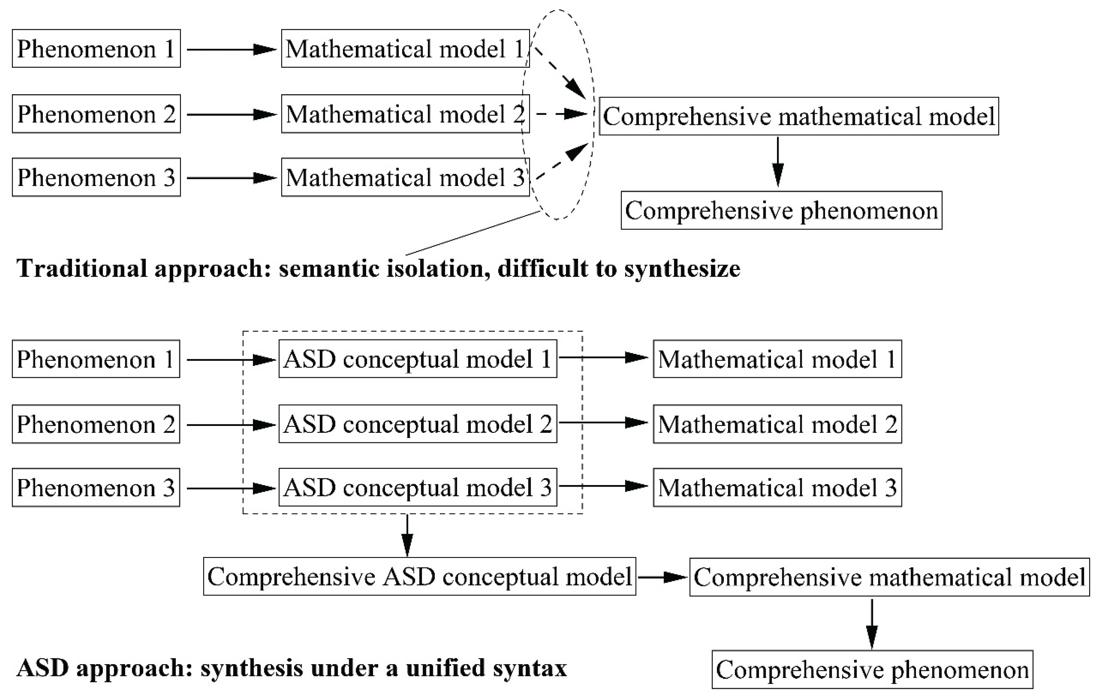
Across these different sub-fields, the scale of the study object, the specific characteristics of interest (target parameters), and the factors inducing change (internal and external actions) often overlap or diverge. Furthermore, terminology varies significantly between domains. Consequently, the traditional path lacks a unified logical and semantic foundation for interdisciplinary research. Mathematical models from different fields suffer from semantic incompatibility and even incommensurability, rendering formal comparison and synthesis difficult, as illustrated in Figure 5.
5.2. The Conceptual Model as a Semantic Bridge
ASD addresses this incommensurability by introducing a "Conceptual Model" layer between the raw phenomenon and the mathematical implementation. By utilizing the formal syntax of "State-Action-State Increment", ASD reduces distinct phenomena to generalized constitutive relations that possess a unified structure.
Serving as a medium for semantic abstraction, the conceptual model allows researchers to define the relationships between the system, its actions, and its state changes at a strictly logical level. This provides a common starting point for diverse phenomenological models. The workflow of ASD operates bidirectionally to achieve semantic alignment:
- Forward Path: Phenomenon → Conceptual Model (Semantic Abstraction) → Mathematical Model (Quantitative Implementation).
- Reverse Path: Existing Mathematical Model → Conceptual Model (Semantic Extraction).
Through this bidirectional mechanism, mathematical models from different sub-fields can be aligned semantically. At the conceptual model level, researchers can explicitly compare and define key elements: system division and boundaries, characteristic time scales, the selection of target parameters, methods of state quantification, and the decomposition of actions. These elements constitute a comparable space, enabling mathematical models that were originally independent and terminologically incommensurable to be analyzed, compared, and synthesized within a unified logical structure (Figure 5).
The detailed scientific research workflow under the ASD framework (specifically the Forward Path) can be summarized as follows:
-
Phenomenon Identification and System Division:
- ∘
- Define the object of study and its boundaries.
- ∘
- Establish the system's spatial scale and the observational time scale.
- ∘
- Identify the research objective and select appropriate target parameters.
-
Conceptual Modeling:
- ∘
- Clarify the logical distinction between internal and external actions and determine the decomposition method for these actions.
- ∘
- Establish the generalized constitutive relations for all identified actions.
-
Mathematical Modeling:
- ∘
- Determine the quantification methods for both state and action (e.g., selecting state parameters and external action paths).
- ∘
- Guided by the conceptual model, establish the specific mathematical expressions for all generalized constitutive relations.
- ∘
- Explicitly define the meaning of each parameter within these mathematical expressions.
-
Model Validation and Refinement:
- ∘
- Calibrate parameters and validate the mathematical model's rationality through experiments or numerical computation.
- ∘
- If systematic deviations occur that cannot be eliminated by parameter correction, return to the Mathematical Modeling stage or, if necessary, the Conceptual Modeling stage.
- ∘
- Continuously engage in an iterative cycle of refinement between Conceptual Modeling and Mathematical Modeling.
5.3. Modularity and the "Platform" Approach
ASD operates as a standardized "platform" or "interface"—anchored by the generalized constitutive relation—into which various mathematical sub-models can be "plugged in" as modular components.
As demonstrated in the illustrative examples of Section 4, the ASD conceptual models are not inherently complex; yet, extremely rich mathematical models and theories can be derived from these simple foundations. Under the ASD framework, these theories are not fundamentally different paradigms, but simply different combinations of components plugged into the same conceptual model.
This inherent modularity clarifies that the complexity of a final mathematical model may arise not from a complex systemic structure, but from the complexity of the specific functions chosen to instantiate the generalized constitutive relations. ASD allows researchers to manage this complexity by isolating it within specific modules. Therefore, ASD does not aim to replace existing scientific laws, but rather to organize them within a unified axiomatic structure.
6. implications and limitations
6.1. Methodological and Philosophical Implications
6.1.1. Ontological State and Epistemological Parameter: A Fundamental Distinction
The distinction between the ontological state and the epistemological parameter is a fundamental philosophical contribution of ASD. While drawing upon the state-space concepts of control theory, ASD posits that a system's true state—its underlying ontological reality—may be complex enough to be unquantifiable by a finite set of known, measurable Parameters.
This perspective significantly expands the theoretical applicability of ASD. It allows the framework to not only unify the mathematical descriptions of known systems (where the state can be fully described by parameters), but also to provide a consistent research methodology for systems awaiting identification. ASD ensures that scientific inquiry maintains a coherent logical structure and a consistent syntax of inference even when operating in an unknown state space. Philosophically, ASD establishes a new epistemology of system modeling, formalizing scientific modeling as a strictly logical behavior and integrating the formation of scientific theories within a formal axiomatic system.
6.1.2. Axiom 2 and the Non-Arbitrary System Boundary
The delineation of a system's boundary often involves a degree of arbitrariness. Axiom 2 provides a metaphysical criterion for correct boundary partition: the boundary is correctly drawn if and only if the resultant internal action is uniquely and deterministically derived from the system's state.
This criterion functionally shifts the system boundary problem to the quantification of state and action. Although quantification remains challenging, Axiom 2 provides a clear heuristic for model development: if the system's response under internal action appears random or indeterminate, it logically implies one of two possibilities: either the system's state has not been fully determined (an incomplete state parameter set), or the action in question includes an external component that has been incorrectly classified.
6.1.3. The B-A Principle and the Logic of Control Experiments
The B-A Principle formalizes the logic of control experiments by defining the net effect of the external action as the difference between the total state change and the change under only the internal action. This comparison provides an axiomatic basis for a formalized superposition principle, crucial for separating the system's self-evolution (state creep) from the externally induced change.
6.1.4. Fulfilling the Vision of General Systems Theory (GST)
ASD represents a decisive attempt to fulfill the original, ambitious vision of GST. GST's initial goal was to establish a universal, trans-disciplinary language to study common laws across all systems.
However, as systems science specialized, this ideal waned, leaving a persistent lack of a rigorous, formalized, and universally applicable framework even for hard systems. ASD provides this essential formal framework and language for hard systems, thereby filling the vacuum left by the incomplete realization of GST's founding ambition. It offers a fully formalized, yet flexible, mechanism for achieving cross-disciplinary semantic alignment by defining a common syntax for causality across fields from physics to engineering.
6.2. Limitations of the Current Framework and Future Directions
The ASD framework proposed herein focuses primarily on the dynamic description of individual systems. While inter-system interactions are deterministically governed by their respective states, modeling large-scale collectives with complex interaction topologies requires the integration of additional mathematical tools. Future research must extend ASD to establish a formalized analytical framework for the complex behaviors central to systems science, including multi-level feedback, emergence, and self-organization.
Furthermore, the current formulation of ASD is validated primarily through physical "hard" systems. While "soft" systems (social, ecological, management) and stochastic systems can theoretically be described as deterministic via metaphysical generalized constitutive relations, significant methodological challenges remain:
- Soft Systems: Parameters in these domains often possess a high degree of subjectivity and complexity (e.g., "satisfaction"), rendering them difficult to quantify with standard scientific instrumentation. Consequently, determining the Ontological State of such systems presents a significant measurement challenge that requires new quantification methodologies.
- Stochastic Systems: For systems exhibiting inherent randomness, a potential resolution is to encapsulate randomness as an intrinsic property of the state itself. Under this paradigm, parameters are treated as probability distributions rather than scalar values. The evolution of the system's state (the distribution) remains deterministic, even if the specific physical manifestation is probabilistic.
Addressing the rigorous quantification of soft states and the formalization of stochastic state evolution remain open areas for further investigation.
7. Conclusions
This study introduced Axiomatic System Dynamics (ASD), a novel, formally self-consistent, and universal framework for the systematic description of evolutionary processes of diverse objects across scientific disciplines. Grounded in three fundamental axioms, ASD establishes a unified conceptual architecture, creating a critical, formal bridge between observed phenomena and their mathematical expressions. This structural alignment directly addresses the persistent challenge of incommensurability, positioning ASD as a foundational step toward a rigorous, trans-disciplinary scientific language.
The efficacy and broad generality of the ASD framework were validated through three progressively complex, illustrative applications:
- Newtonian Particle Mechanics: Demonstrated the framework's capacity to model elementary dynamics, formally re-conceptualizing inertia as the system's Internal Action and linear motion as its inherent state creep.
- Material Stress-Strain Constitutive Relations: Validated the application to Non-Markovian systems, highlighting how the generalized state parameter formally incorporates history-dependence, thus providing a rigorous axiomatic home for system "memory."
- Saturated Soil Consolidation: Demonstrated the framework's effectiveness in handling multi-scale, multi-mechanism coupled systems. This application illustrated the crucial point that the partition of actions (internal vs. external) is not intrinsic but is fundamentally dictated by the research objective, provided it strictly adheres to Axiom 2.
While ASD provides a robust formalization for a broad range of deterministic physical systems, this work represents an initial endeavor. Future investigations must substantially extend the framework’s rigor to more challenging domains, specifically by developing formal methodological structures for confronting large interacting systems, soft systems (where state quantification is inherently difficult), and inherently stochastic systems. Ultimately, the principles established by ASD offer a valuable conceptual and formal reference point for advancing the goal of scientific methodological unification.
Data Availability Statement
Data will be made available on request.
Acknowledgments
This research was supported by the Natural Science Foundation of Zhejiang Province (LZ24E080002), which is gratefully acknowledged.
Conflicts of Interest
The author declare that they have no known competing financial interests or personal relationships that could have appeared to influence the work reported in this paper.
References
- Ashby, W. R. (1956). An introduction to cybernetics.
- Baligh, M. M., & Levadoux, J. N. (1978). Consolidation theory for cyclic loading. Journal of the Geotechnical Engineering Division, 104(4), 415-431. [CrossRef]
- Cabrera, D., Cabrera, L. L., & Midgley, G. (2023). The four waves of systems thinking. Journal of Systems Thinking, 1-51. [CrossRef]
- Checkland, P., & Poulter, J. (2020). Soft systems methodology. In Systems approaches to making change: A practical guide (pp. 201-253). London: Springer London.
- Chen, C. T. (1984). Linear system theory and design. Saunders college publishing.
- Dill, E. H. (2006). Continuum mechanics: elasticity, plasticity, viscoelasticity. CRC press. [CrossRef]
- Guerriero, V., & Mazzoli, S. (2021). Theory of effective stress in soil and rock and implications for fracturing processes: a review. Geosciences, 11(3), 119. [CrossRef]
- Guerriero, V. (2022). 1923–2023: one century since formulation of the effective stress principle, the consolidation theory and Fluid–Porous-Solid interaction models. Geotechnics, 2(4), 961-988. [CrossRef]
- Hill, R. (1998). The mathematical theory of plasticity (Vol. 11). Oxford university press.
- Holtz, R. D., Kovacs, W. D., & Sheahan, T. C. (1981). An introduction to geotechnical engineering (Vol. 733). Englewood Cliffs, NJ: Prentice-hall.
- Islam, M. N., & Gnanendran, C. T. (2017). Elastic-viscoplastic model for clays: Development, validation, and application. Journal of Engineering Mechanics, 143(10), 04017121. [CrossRef]
- Jackson, M. C. (2016). Systems thinking: Creative holism for managers. John Wiley & Sons, Inc.
- Jackson, M. C. (2019). Critical systems thinking and the management of complexity. John Wiley & Sons.
- Kauffman, S. A. (1992). The origins of order: Self-organization and selection in evolution. In Spin glasses and biology (pp. 61-100).
- Khan, A. S., & Huang, S. (1995). Continuum theory of plasticity. John Wiley & Sons.
- Lai, W. M., Rubin, D., & Krempl, E. (2009). Introduction to continuum mechanics. Butterworth-Heinemann.
- Midgley, G. (2000). Systemic intervention. In Systemic intervention: Philosophy, Methodology, and practice (pp. 113-133). Boston, MA: Springer Us. [CrossRef]
- Radhika, B. P., Krishnamoorthy, A., & Rao, A. U. (2020). A review on consolidation theories and its application. International Journal of Geotechnical Engineering, 14(1), 9-15. [CrossRef]
- Richardson, G. P. (2011). Reflections on the foundations of system dynamics. System dynamics review, 27(3), 219-243. [CrossRef]
- Rousseau, D. (2015). General systems theory: Its present and potential. Systems Research and Behavioral Science, 32(5), 522-533. [CrossRef]
- Rousseau, D. (2017). Systems research and the quest for scientific systems principles. Systems, 5(2), 25. [CrossRef]
- Sterman, J. (2018). System dynamics at sixty: the path forward. System Dynamics Review, 34(1-2), 5-47. [CrossRef]
- Suh, N. P. (1998). Axiomatic design theory for systems. Research in engineering design, 10(4), 189-209.
- Terzaghi, K. (1925). Principles of soil mechanics. IV. Settlement and consolidation of clay. Engineering News-Record, 95, 874.
- Terzaghi, K. (1943). Theoretical soil mechanics.
- Terzaghi, K., Peck, R. B., & Mesri, G. (1996). Soil mechanics in engineering practice. John wiley & sons.
- Thurner, S., Hanel, R., & Klimek, P. (2018). Introduction to the theory of complex systems. Oxford University Press.
- Von Bertalanffy, L. (1968). General system theory. New York, 41973(1968), 40.
- Wilson, N. E., & Elgohary, M. M. (1974). Consolidation of soils under cyclic loading. Canadian Geotechnical Journal, 11(3), 420-423. [CrossRef]
- Yin, J. H., & Graham, J. (1994). Equivalent times and one-dimensional elastic viscoplastic modelling of time-dependent stress–strain behaviour of clays. Canadian Geotechnical Journal, 31(1), 42-52. [CrossRef]
- Yin, J. H., & Graham, J. (1996). Elastic visco-plastic modelling of one-dimensional consolidation. Geotechnique, 46(3), 515-527. [CrossRef]
- Yin, J. H., & Graham, J. (1999). Elastic viscoplastic modelling of the time-dependent stress-strain behaviour of soils. Canadian geotechnical journal, 36(4), 736-745. [CrossRef]
- Ying-chun, Z., & Kang-he, X. (2005). Study on one-dimensional consolidation of soil under cyclic loading and with varied compressibility. Journal of Zhejiang University-SCIENCE A, 6(2), 141-147. [CrossRef]
Figure 1.
Stress path and strain path of material element.
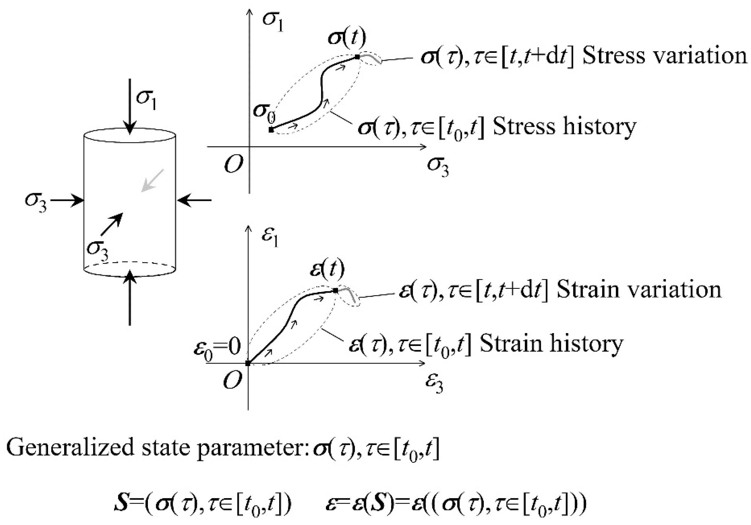
Figure 2.
Generalized state parameter in different models.
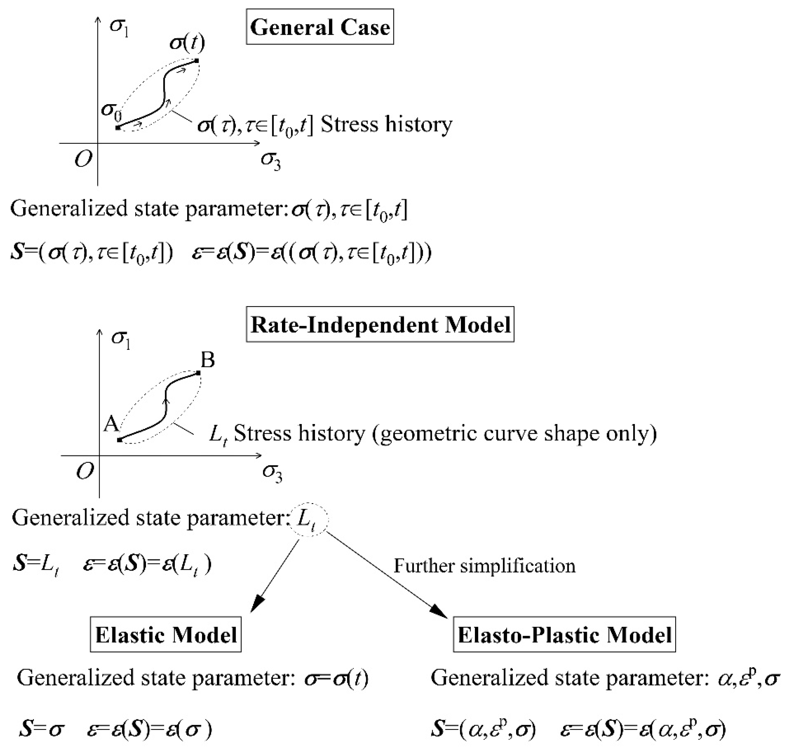
Figure 3.
Soil sample system and soil element subsystem.
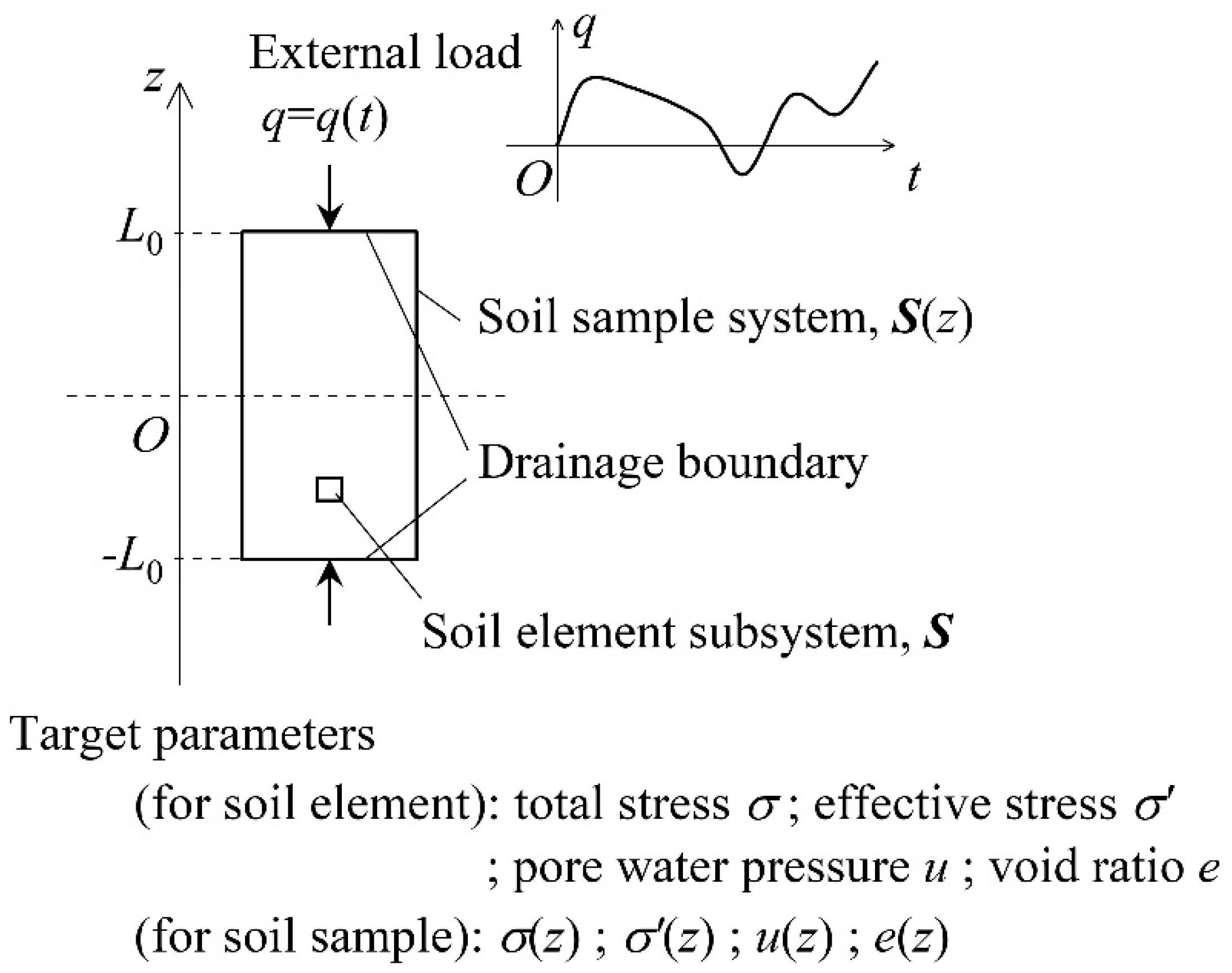
Figure 4.
ASD conceptual model for one-dimensional consolidation.
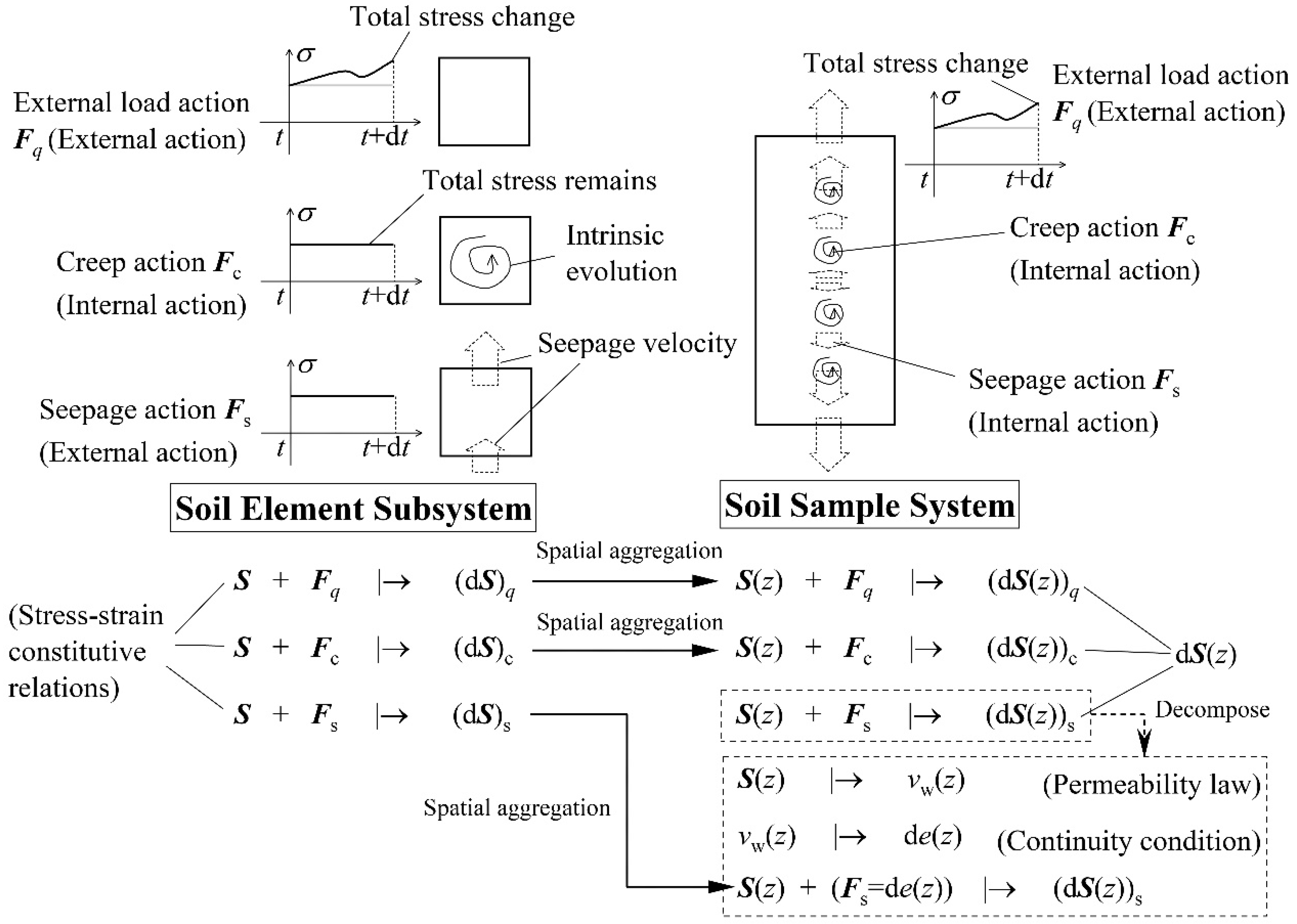
Figure 5.
Traditional and ASD approaches of modeling.
Disclaimer/Publisher’s Note: The statements, opinions and data contained in all publications are solely those of the individual author(s) and contributor(s) and not of MDPI and/or the editor(s). MDPI and/or the editor(s) disclaim responsibility for any injury to people or property resulting from any ideas, methods, instructions or products referred to in the content. |
© 2025 by the authors. Licensee MDPI, Basel, Switzerland. This article is an open access article distributed under the terms and conditions of the Creative Commons Attribution (CC BY) license (http://creativecommons.org/licenses/by/4.0/).
Copyright: This open access article is published under a Creative Commons CC BY 4.0 license, which permit the free download, distribution, and reuse, provided that the author and preprint are cited in any reuse.


