
Submitted:
20 November 2025
Posted:
20 November 2025
You are already at the latest version
Abstract
Plastic pollution in aquatic environments is a major ecological problem requiring scalable autonomous solutions for cleanup. This study addresses the coordination of multiple Autonomous Surface Vehicles by formulating the problem as a Partially Observable Markov Game and decoupling the mission into two tasks: exploration, to maximize coverage, and cleaning, to collect trash. These tasks share navigation requirements but present conflicting goals, motivating a multi-objective learning approach. The proposed multi-agent deep reinforcement learning framework involves the utilisation of the same Multitask Deep Q-network shared by all the agents, with a convolutional backbone and two heads, one dedicated to exploration and the other to cleaning. Parameter sharing and egocentric state design leverages agent homogeneity and enable experience aggregation across tasks. An adaptive mechanism governs task switching, combining task-specific rewards with a weighted aggregation and selecting tasks via a reward-greedy strategy. This enables the construction of Pareto fronts capturing non-dominated solutions. The framework surpasses existing algorithms in the literature, improving hypervolume and uniformity metrics by 14 % and 300 %, respectively. It also adapts to diverse initial trash distributions, providing decision-makers with a portfolio of effective and adaptive strategies for autonomous plastic cleanup.
Keywords:
multi-task multi-agent deep reinforcement learning
; multi-objective optimization
; autonomous surface vehicles
; environmental monitoring
; partially observable markov games
1. Introduction
Macro-plastic (plastic >25 mm) persists in aquatic environments, threatening ecosystems through entanglement, ingestion, and the trophic transfer of toxic additives [1,2]. Despite advances in mitigation and cleanup technologies using Autonomous Surface/Unmanned Surface Vehicles (ASVs/USVs) [3,4,5,6], a primary challenge in plastic cleanup missions remains the uncertainty of trash distribution before deployment [7,8,9]. Plastic contamination is highly dynamic—driven by water currents, wind, and human activity—which undermines static trajectory planning and limits the efficiency of deterministic control or classical optimization approaches. Recent advances in Deep Reinforcement Learning (DRL) have demonstrated the capacity to handle such uncertainty by enabling adaptive, data-driven decision-making. Canonical methods such as Deep Q-Learning (DQL) [10] and its extensions like Rainbow DQN [11] have shown strong performance in high-dimensional control tasks, including pollution monitoring [12,13,14] and trash collection [9]. To extend these capabilities to coordinated multi-robot systems, we model the cleanup mission as a Partially Observable Markov Game (POMG) [15], which naturally captures both the uncertainty of trash locations and the interactions among multiple ASVs operating simultaneously. The POMG generalizes the classical Markov Decision Process (MDP) to multi-agent scenarios where each vehicle receives only partial observations of the environment, reflecting realistic sensing and communication constraints. POMG thereby provides a mathematical foundation for Multi-Agent DRL (MADRL), which leverages parameter sharing to improve scalability and coordination across ASV fleets [16,17].
To manage mission complexity, we decouple the mission into two distinct tasks: exploration, where agents aim to cover the map to localize trash, and cleaning, where they focus on trash collection. Multi-task learning has been used in this context to jointly optimize policies for both objectives using Multi-task DQN (MDQN) architectures [7,8,18]. Unlike prior studies that relied on fixed-phase strategies, conducting exploration first and cleaning afterward [8], we treat task allocation as a dynamic decision variable. Specifically, a binary switch variable enables each agent to adaptively select between exploratory and cleaning policies. Therefore, agents can shift toward cleaning when nearby plastic concentrations are high or return to exploration when the local area becomes depleted. This flexible task allocation introduces an inherent trade-off: excessive exploration reduces cleaning time, while insufficient exploration risks leaving undetected debris.
The use of Multi-Objective DRL (MO-DRL) has gained increasing attention for resolving trade-offs between conflicting objectives. Foundational studies such as [19,20], and [21] developed techniques for learning Pareto-optimal policies through scalarization and preference-conditioned networks. Building on these ideas, by training across varying allocations of , we construct Pareto-optimal fronts that capture the trade-offs between exploration coverage and cleaning efficiency. To support adaptive decision-making, we also introduce a reward-greedy policy selection mechanism inspired by submodular optimization principles [22,23]. This mechanism evaluates all possible task assignments across the fleet and selects the one that maximizes a weighted combination of exploration and cleaning performance. By systematically varying the weights, the framework reconstructs a diverse Pareto front, providing decision-makers with a portfolio of strategies tailored to different mission priorities. In summary, we adopt a Multi-Task Multi-Agent DRL (MT-MADRL) framework solved via multi-objective optimization. Our contributions are twofold: (i) a multi-task multi-agent DRL framework for ASV-based plastic cleanup that decouples exploration and cleaning while enabling adaptive task switching; (ii) a multi-objective optimization formulation that leverages reward decomposition and Pareto front construction to balance exploration and cleaning under diverse mission requirements.
The rest of this papers continues as follows: sec:materials introduces the environmental framework, including the scenario characteristics, system dynamics, and the methodology used throughout the study. It also describes the DRL formulation, the policy network architecture and training procedure, the state and reward definitions, and the proposed policy-selection mechanism. sec:Results details the simulation setup and presents the experimental results, including a comparison between the proposed method and existing approaches in the literature. Finally, sec:conclu provides concluding remarks and outlines directions for future research.
2. Materials and Methods
2.1. Problem Formulation
We formulate the plastic cleanup mission as a POMG [24] involving N homogeneous ASVs operating in a discretized aquatic environment. The POMG framework naturally captures the agents’ limited perception and the interactions among multiple ASVs. The overall mission objective is to remove trash as efficiently as possible, which implicitly requires effective coordination, safe navigation, and energy-aware trajectories. In order to locate and remove trash items, it is necessary to explore the environment. Rather than considering this as an implicit part of the cleaning process, we have decided to decouple the learning process into two dedicated policies: an exploration policy, where agents aim to maximize coverage of the environment, and a cleaning policy, where agents collect as much identified trash as possible once locations are known. Both tasks share underlying requirements such as efficient navigation and obstacle avoidance, yet they present conflicting objectives: allocating more effort to exploration improves trash localization but reduces the time available for collection, while prioritizing cleaning without sufficient exploration leads to incomplete recovery. This inherent tension motivates a multi-objective learning framework.
Formally, let denote a policy and let D be the number of objectives. Each policy produces a vector of performance metrics across episodes due to stochastic trash distributions. The expected performance is , where . In our case, , with and representing expected exploration and cleaning performance, respectively. A policy is Pareto-optimal if there is no other policy such that:
The aim of this work is thus twofold: (i) to learn specialized exploration and cleaning policies, and (ii) to construct a Pareto front of solutions that captures the optimal trade-offs between the two objectives.
2.2. Scenario and Vehicle Properties
Let denote a grid-based map of size structured as a connected graph, where
is the set of nodes, with each node corresponding to a location in the grid. The set of edges connecting adjacent nodes is denoted as , indicating possible movements between neighboring nodes. Each node connects to its eight immediate neighbors, making the grid eight-connected. Nodes with fewer than eight connections represent the presence of obstacles. The graph G can also be represented as a binary matrix of size (see Figure 1):
Let N denote the number of ASVs. The fleet position in G at time t is given by , where is the position of vehicle n. ASVs move synchronously in one of the eight cardinal directions (N, E, S, W, NE, SE, NW, SW), with each simulation step corresponding to one discrete movement. Actions leading to non-navigable nodes () are masked to ensure valid transitions. When multiple ASVs attempt to occupy the same node, conflicts are resolved via a consensus algorithm [25], preventing inter-vehicle collisions. Battery life imposes a mission length constraint, defined by the maximum traversable distance under a fully charged battery. Each ASV is also equipped with a camera. The perception area of vehicle n is defined as:
where is the vision radius and denotes Euclidean distance (see Figure 2).
2.3. Trash dynamics and recollection
Let denote the set of trash positions, where K is the total number of items and are continuous coordinates. At the beginning of each episode, trash is generated in 1–10 clusters, with items sampled from a multivariate normal distribution. The dynamics of each item follow:
where is sampled once per episode, and is sampled independently at each step. Weights are fixed at and . Trash items are discretized into a matrix (see Figure 1 and Figure 2), where:
with denoting the region corresponding to cell . Each agent maintains an estimated trash map , initialized to zero and updated whenever :
Agents share their observations via centralized communication, mitigating some limitations of partial observability but still subject to the uncertainty of trash dynamics. When an ASV occupies , it collects all trash at that node, with collection capacity assumed unlimited. The number of items collected is:
2.4. Deep Reinforcement Learning Framework
Reinforcement Learning (RL) [26] addresses sequential decision-making by modeling the interaction between agents and the environment as a MDP . At each step t, an agent observes a state , selects an action , transitions to , and receives a reward . The objective is to learn a policy that maximizes the expected cumulative reward. Q-Learning estimates the action-value function , the expected return of taking action a in state s under . Deep Q-Networks (DQNs) [10] approximate with a neural network parameterized by , updated via:
where is the learning rate. Stability and performance are enhanced through mechanisms such as Experience Replay, Target Networks, Double DQN [27], and the Dueling Architecture [28].
MADRL generalizes DQL to a cooperative setting with N homogeneous agents acting in a shared environment, formalized as a POMG . Each agent receives a local observation , selects an action , and receives a reward , while the environment evolves according to the joint action . Each agent aims to maximize its long-term return:
where denotes all agents except n. In our cooperative ASV cleanup scenario, parameter sharing [29] is applied: all agents use the same policy network, allowing experiences to be aggregated, reducing computational cost, and ensuring scalability. To improve credit assignment, agents are rewarded based on their individual contributions to the team’s performance [30].
To further improve learning, the mission is formulated as a multi-task problem with two tasks: exploration, which aims to maximize coverage and locate trash, and cleaning, which focuses on collecting the identified trash. While the state and action spaces are shared, transition dynamics and rewards differ per task , producing a vectorized reward signal. Following [18], Multi-task Deep Q-Networks (MDQN) employ separate Q-heads per task while sharing the underlying feature representation. This allows knowledge gained in exploration, such as efficient navigation and obstacle avoidance, to transfer to cleaning, improving overall mission performance.
2.5. Policy Network Training
2.5.1. Phase Construction
Following [7], the mission is divided into two phases to handle initially unknown trash locations: Exploration and Cleaning. The transition between phases is controlled by a variable , representing the probability of selecting an exploration action:
where and are the Q-functions for exploration and cleaning, respectively. In the Exploration phase, at every step, so all actions are chosen according to the exploratory policy , with the primary goal of maximizing map coverage and discovering trash locations. In the Cleaning phase, , so actions are fully governed by the cleaning policy , aiming to recollect the detected trash efficiently.
2.5.2. States
The state representation for agent n is egocentric and composed of three min-max normalized channels:
- Trash model: , shared among all agents, representing detected trash positions and capturing partial observability.
- Agent trail position: records the agent’s detection history over the past 10 steps, with current detection cells at 1 and past steps decaying by 0.1 per step, down to 0.1.
- Position of other agents: the union of detection masks of all other agents, with cells inside the masks set to 1, providing awareness of fleet distribution.
2.5.3. Rewards
At each step t, each agent n receives a vector of two rewards , corresponding to exploration and cleaning objectives.
The Exploration Reward () encourages discovery of new areas while penalizing inactivity and redundancy:
- Visit reward: proportional to newly discovered cells, shared among overlapping agents:where counts overlapping coverage.
- Inactivity penalty: penalizes consecutive steps without discovering new areas:where accumulates the number of consecutive steps without discovering new cells, and scales this penalty to control its impact.
- Redundancy penalty: penalizes overlap with areas explored by self or other agents in the last steps:
The Cleaning Reward () encourages trash collection and efficient movement towards trash:
- Trash collection reward: rewards collecting trash at current position.
- Distance reward: promotes movement towards nearby trash using inverse Dijkstra distances:
- Model update reward: encourages adaptation to dynamic trash movement.
- Time penalty: discourages unnecessary delays.
2.5.4. Multi-task Policy Network
The network containing the two task policies is trained following the Randomized -Sampling for Pareto Front Approximation Algorithm as in [8]. All agents share a single MDQN-based policy network composed of a dense Convolutional Neural Network (CNN) with two dueling Q-heads, one for exploration and one for cleaning. Parameter sharing is employed because the agents are homogeneous in both observations and actions, while the egocentric state formulation ensures scalability to an arbitrary number of agents. Each Q-head is trained independently using its respective task-specific rewards through DQL.
The utilisation of shared layers facilitates the aggregation of experiences derived from both tasks, thereby reducing computational cost and enhancing sample efficiency. In order to ensure diverse learning across the exploration–cleaning trade-off, the duration of the exploration phase is sampled at the beginning of each episode. This duration determines when transitions from 1 (pure exploration) to 0 (pure cleaning) over the course of the mission. By varying the phase length across episodes, the network learns policies covering the full spectrum of task allocations. At the end of training, the network contains two fully trained policies, exploration and cleaning .
2.6. Reward-Greedy Policy Selection and Pareto Front Construction
To enhance adaptive decision-making, we introduce a Reward-Greedy Policy Selection (RGPS) mechanism. At each decision step, RGPS evaluates all possible task allocations across the fleet, specifically, whether each ASV should perform exploration or cleaning. Given two possible tasks per vehicle, this results in possible task combinations for a fleet of N ASVs. Each combination is simulated to compute its expected scalarized reward, which aggregates exploration and cleaning objectives according to a given weighting of objectives. The combination yielding the highest weighted reward is selected, and each agent executes the corresponding action from its designated policy (exploration or cleaning). This process defines the fleet’s joint behavior at every step. The RGPS mechanism follows the principle of greedy submodular optimization, which is well-established for near-optimal decision-making in adaptive and stochastic settings [22,23]. In submodular systems, greedy maximization provides strong theoretical guarantees for solution quality under uncertainty—properties that align well with our partially observable and dynamically changing aquatic environment. Since the marginal benefit of additional exploratory actions typically diminishes as more trash is detected, the problem exhibits approximately submodular behavior. The Reward-Greedy method is simple to implement and it does not require additional learning. It explicitly considers all feasible task assignments, ensuring near-optimal short-term decisions based on the chosen reward weighting. Moreover, it leverages the separate training of exploration and cleaning policies, allowing agents to specialize while maintaining coordination. Figure 3 shows the diagram that summarizes our proposed algorithm.
Weighting Method: To balance exploration and cleaning, we introduce a weighting coefficient that combines the two objectives into a single scalar optimization function. This methods allow the user to specify preferences, which may be articulated in terms of goals or the relative importance of different objectives. Following the most common general scalarization methods for multi-objective optimization[31], with and , the combined objective can be expressed using either:
- Weighted Sum (WS): the most common approach to multi-objective optimization is the weighted sum method, which is essentially a convex combination of the two rewards, it suffers from the disadvantage of not being able to find a diverse set solutions if the Pareto front is non-convex.
- Weighted Power (WP): In this method, each reward is raised to a power before applying the weight. This allows emphasizing certain objectives non-linearly and can be tuned via the parameter :
- Weighted Product of Powers (WPOP): This multiplicative approach combines the rewards by taking each reward to the power of its respective weight and then multiplying them. It is useful for emphasizing that all objectives should be high, as a low value in any objective strongly reduces the total scalarized reward:
- Exponential Weighted Criterion (EWC): In response to the inability of the weighted sum method to capture points on non-convex portions of the Pareto optimal surface, [32] propose the exponential weighted criterion, the performance of the method depends on the value of p and usually a large value of p is needed.
These formulations provide a flexible trade-off between the two competing objectives, enabling systematic exploration of the Pareto front. The RGPS mechanism uses this weighted reward to evaluate all possible policy assignments, selecting the combination that maximizes at each step. By repeating this process across different weightings w and multiple episodes, we obtain a set of policies whose expected performance in exploration and cleaning spans the trade-off space. Plotting the expected versus for these policies forms a Pareto front, representing the set of non-dominated strategies. Decision-makers can then select policies from the Pareto front according to mission priorities, ensuring an explicit balance between maximizing trash collection and achieving full coverage of the environment.
3. Results
The proposed algorithm has been implemented in Python1 3, using the PyTorch2 library for policy optimization. The Gym3 has been used to simulate the environment, NumPy4 and SciPy5 libraries for numerical and matrix operations. Pareto Fronts were constructed using Pymoo6. The algorithm’s code and results are accessible in a GitHub repository7. All experiments and simulations were run on an Intel Xeon Gold 5220R CPU operating at 2.20GHz with 187GB of RAM. Additionally, a NVIDIA GeForce RTX 3090 GPU with 24GB of VRAM was employed to accelerate training.
3.1. Simulation Settings
The environment consists of four ASVs, each equipped with a detection radius of 2 nodes, a movement budget of 200 units per episode, and a movement step size of 1 node. The ASVs start from four fixed initial positions. Horizontal and vertical movements incur a cost of 1 unit, while diagonal movements cost units.
Table 1 lists the summary of the environment and training parameters.
Greedy Execution: The agents are evaluated over 100 episodes using the Reward-Greedy strategy. For each episode, a weight vector is sampled from a uniform distribution , where one weight is drawn and the other is set to , ensuring that the sum of weights equals one. After completing the 100 episodes for a given weight vector, the mean values of the exploration metric (PMV) and the cleaning metric (PTC) are computed. This process is repeated for 100 different weight combinations. Finally, the Pareto Front is constructed from the resulting set of 100 metric pairs. The entire procedure is performed separately for each weight-based scalarization method. The path planner that is going to choose the action once the decision to explore or clean is taken by the RGPS agent, is trained as in [8]
3.2. Metrics
We evaluate the performance of each policy using a set of objective metrics that quantify exploration efficiency and cleaning effectiveness.
- Percentage of the Map Visited (PMV): It is the exploration objective to be maximized, and it measures the percentage of the map that has been visited during the mission. It is defined as the proportion of the total navigable area that has been visited at least once by any ASV. A higher PMV value indicates a more comprehensive exploration, ensuring that the agents gather sufficient information about the environment’s structure, obstacles, and trash distribution, which is crucial for the subsequent cleaning phase. Mathematically, PMV is given by:
- Percentage of Trash Cleaned (PTC): It is the cleaning objective to be maximized, and it measures the proportion of trash that has been effectively eliminated from the environment, relative to the total amount of trash present present at the beginning of the episode (K). Optimizing PTC requires efficient path planning and coordination among agents to maximize trash collection before exceeding their distance limits. PTC is mathematically defined as:
To characterize the trade-offs between these objectives, we compute Pareto front metrics that capture the diversity, extension and quality of the resulting solutions.
-
Consecutive Spacing: The spacing metric measures the variance of distances between consecutive solutions along the Pareto front, sorted by the first objective . It captures gaps along the front better than nearest-neighbor spacing in 2D.For a sorted Pareto front , the consecutive distances areand the spacing metric is defined as the standard deviation of these distances:whereA lower S indicates more uniform spacing along the front.
-
Zitzler’s M3 Metric: The M3 metric measures the extent of the Pareto front along all objectives. For a Pareto front in m objectives, letbe the range of the front along the i-th objective. Then the M3 metric is defined asA higher indicates a larger extent of the front across all objectives.
- Hypervolume (HV): The hypervolume quantifies the size of the objective space dominated by the Pareto Front (PF) with respect to a reference point . For discrete non-dominated points sorted by (e.g., PTC), the hypervolume can be approximated as the sum of rectangular areas between consecutive PF points:where and denote the objective values of the i-th non-dominated solution in the sorted PF, and corresponds to the reference point. A higher indicates a larger and more dominant Pareto region, reflecting both convergence and diversity.
3.3. Scalarisation Results
As illustrated in Figure 4, the Pareto fronts obtained for each scalarization method under the Reward-Greedy Policy Selection (RGPS) framework are presented, in conjunction with the combined Pareto set which integrates all scalarizations to exploit the complete information available. The corresponding performance metrics are summarised in Table 2.
It is evident that the WP method exhibits significantly poorer performance in comparison to the alternative approaches. The Wilcoxon signed-rank test, conducted between Pareto fronts, revealed that the remaining methods do not exhibit statistically significant differences (Table 3). The WS approach achieves the highest hypervolume; however, it is known that it is limited to convex regions of the Pareto front. In contrast, the WPOP and EWC methods, both non-linear scalarisations, achieve slightly lower hypervolume and Pareto extension () values but yield improved Spacing due to their ability to explore non-convex regions. Furthermore, due to the convex-constrained nature of WS, numerous weight combinations tend to converge towards the boundary of the front, thereby leading to elevated values.
When all scalarization results are combined, the best overall metrics are achieved, along with an increased number of Pareto-optimal points. Figure 4 illustrates the contribution of each scalarization method to the combined Pareto front. Out of 40 total Pareto points, EWC contributes the majority (47.50%), followed by WS (27.50%) and WPOP (25.00%), while WP does not contribute. This highlights the importance of employing multiple scalarization techniques of distinct natures (linear, non-linear, additive, multiplicative, and exponential) to achieve a well-distributed and comprehensive Pareto front. The combined front represents our proposed contribution and will serve as the basis for comparison against alternative algorithms from the literature.
3.3.1. Comparison
For benchmarking against existing approaches, we adopt the methodology introduced in [8], hereafter referred to as the Fixed-Phase Pareto Set (FP2S). A predefined set of phase transition configurations, denoted as the Phase Duration Set (PDS), is used to generate possible phase durations whose candidate policies are later evaluated for Pareto optimality. A value in the PDS represents the proportion of the mission dedicated to the exploration phase. The PDS ranges from 1.0 to 0.0 in decrements of 0.1 (therefore 11 values), forming the sequence:
Here, q represents the step index, ensuring a uniform progression from a mission of pure exploration () to pure cleaning (). For instance, a of 0.3 () means that 30% of the mission corresponds to exploration (all agents executing exploration behavior), followed by 70% cleaning. During training, the network is periodically evaluated under each PDS configuration. If a newly trained policy surpasses the current best for a specific PDS and objective, it replaces the previous one, ensuring that only the most optimal policies are retained for Pareto evaluation. Then, for each selected PDS value, three distinct policies are stored as Pareto candidates every 500 training episodes: 1) Best Cleaning Policy: The policy achieving the highest cleaning performance within that PDS. 2) Best Exploration Policy: The policy attaining the greatest exploration efficiency within that PDS. 3) Final Trained Policy: The policy obtained at the end of training, which may exhibit improved generalization to unseen scenarios due to prolonged optimization.
Once all candidate policies are trained, Pareto optimality is determined through post-training evaluation. Each policy generated from the Phase Duration Set (PDS) is tested on an independent evaluation set consisting of 200 randomized episodes per environment. During this stage, the average PTC and PMV metrics are measured for each policy. These averaged results are used to determine Pareto optimality and construct the final Fixed-Phase Pareto Set with ours.
Table 4 reports the performance of the FP2S policies across different fixed exploration-to-cleaning phase ratios (PDS). Figure 5 presents a comparative analysis between the Pareto Front obtained with our proposed Combined approach and the FP2S baseline from the literature. The front generated by FP2S exhibits a smaller number of Pareto-optimal solutions, concentrated primarily in regions with high exploration but limited cleaning performance. This scarcity of solutions results in a sparser and less continuous front, which ultimately reduces the achievable hypervolume and diversity. In contrast, the Combined Pareto Front (black crosses) demonstrates a much denser and more evenly distributed set of non-dominated policies, extending further along both objective axes. This indicates that our method achieves a broader and more balanced coverage of the trade-off space between exploration and cleaning.
As detailed in Table 2, our approach achieves a significantly higher hypervolume value (5810.03 compared to 5091.75), confirming superior overall performance across both objectives. The improved hypervolume indicates that the Combined Pareto Front dominates a larger portion of the objective space, offering more favorable trade-offs between exploration efficiency and cleaning effectiveness. Furthermore, the Spacing metric decreases substantially (0.70 versus 2.14), showing that the solutions in our front are more uniformly distributed, providing smoother transitions between neighboring policies. This uniformity is desirable for multi-objective decision-making, as it allows for finer granularity when selecting operating points according to specific mission preferences.
The extension metric remains comparable between both methods, although our Combined approach achieves similar coverage with a substantially larger number of points (40 versus 9). This richer set of solutions improves the interpretability and applicability of the Pareto front, giving mission planners a broader range of policies to select from based on operational priorities or environmental conditions. It is worth noting that the FP2S front’s lower diversity is primarily due to its reliance on fixed-duration phase transitions, which limits the variability of exploration–cleaning balance during training. By contrast, our approach combines multiple scalarization strategies of different natures—linear, nonlinear, and exponential—allowing the discovery of policies across a wider spectrum of trade-offs.
Overall, the results clearly demonstrate that the proposed Combined Pareto Front not only surpasses the FP2S baseline in terms of quantitative Pareto metrics but also provides greater adaptability, finer policy resolution, and a more comprehensive representation of the underlying exploration–cleaning dynamics. This enhanced front serves as a more informative and flexible decision-making tool for real-world multi-objective environmental cleanup missions.
Figure 6 illustrates the evolution of task allocations across the four agents for three representative scalarization methods, as well as the evolution produced by FP2S for a given . Each line indicates the instantaneous task selected at each time step ( for exploration, for cleaning). As expected, the EWC configuration (Figure 6), which heavily prioritizes cleaning (, ), produces trajectories dominated by cleaning action selections, reflecting a predominance of cleaning behavior. Conversely, the WS configuration (Figure 6), which emphasizes exploration (, ), results in substantially fewer cleaning action selections, consistent with exploratory dominance. The WPOP configuration (Figure 6) lies between these two extremes, producing a balanced alternation between exploration and cleaning phases. Finally, Figure 6 illustrates FP2S, which—as opposed to the adaptive DRL-based policies—applies a predefined task schedule shared synchronously across all agents, and therefore does not constitute an adaptive policy-switching mechanism. However, the temporal evolution of within each episode reveals that the agents’ task decisions are not trivially determined by the scalarization weights. Even in strongly biased configurations, agents exhibit frequent task switches and non-monotonic trajectories. This behavior can be attributed to the strong interdependence between exploration and cleaning: an agent’s optimal task choice depends not only on its local context but also on the collective state of the environment and the complementary actions of other agents. Consequently, the system demonstrates emergent coordination, where task allocation dynamically adapts to environmental and inter-agent conditions.
4. Conclusions
This work introduces a multi-agent deep reinforcement learning framework for autonomous plastic cleanup using fleets of ASVs. The proposed system formulates the problem as a POMG, decoupling the mission into two complementary tasks: exploration, to map and locate waste, and cleaning, to collect it efficiently. Both tasks share navigation capabilities but involve conflicting objectives, motivating a multi-objective optimization approach. A shared two-headed Deep Q-Network, with one head dedicated to exploration and the other to cleaning, allows all agents to benefit from parameter sharing and experience aggregation, enhancing scalability and training efficiency.
To enhance adaptive decision-making, we introduce the Reward-Greedy Policy Selection (RGPS) mechanism, inspired by the principles of adaptive submodularity [22,23]. RGPS evaluates all feasible task allocations across the fleet at each time step and greedily selects the configuration that maximizes a scalarized reward. This mechanism is computationally efficient, requires no additional training, and explicitly considers the interdependence between agents’ actions. By leveraging separate policies for exploration and cleaning, RGPS enables coordinated yet specialized behavior, making it well suited to the dynamic and stochastic nature of aquatic environments. The proposed approach generates a well-distributed Pareto front, revealing diverse strategies across the exploration–cleaning spectrum. Compared to the Fixed-Phase Pareto Set (FP2S) baseline from the literature, our framework achieves a 14% improvement in hypervolume and a 300% increase in uniformity, confirming superior Pareto coverage and policy diversity. Moreover, the system exhibits adaptive behavior across environments of different scales, automatically adjusting phase durations to maximize mission efficiency.
Future work will focus on developing more computationally efficient approaches for constructing Pareto fronts, such as Multi-Objective Evolutionary Algorithms (MOEAs), which can evolve a diverse set of trade-off solutions over successive generations. Another promising direction is to incorporate mission duration as an additional objective, thereby extending the optimization to a three-dimensional Pareto front that captures the interplay between exploration, cleaning, and time efficiency. Moreover, adaptive mechanisms capable of dynamically adjusting the exploration–cleaning balance based on real-time environmental feedback could be explored. This adaptability could be realized through Hierarchical Reinforcement Learning (HRL), where a high-level policy governs the switching between tasks, while low-level controllers handle task-specific decision-making.
Author Contributions
Conceptualization, S.D., Y.S and G.D; methodology, S.D., Y.S. and G.D; software, S.D. and Y.S.; validation, S.D., Y.S. and G.D; formal analysis, S.D., Y.S. and G.D; investigation, S.D.; resources, G.D and T.S.; writing—original draft preparation, S.D.; writing—review and editing, S.D., Y.S., G.D , T.S. and P.M.; visualization, S.D.; supervision, Y.S., G.D , T.S. and P.M.; project administration, G.D and T.S.; funding acquisition, G.D and T.S. All authors have read and agreed to the published version of the manuscript.
Funding
This research was funded by the Spanish Ministry of Science, Innovation, and Universities MICIU/AEI/10.13039/501100011033, by FEDER and by the European Union EU under grant PID2024-158365OB-C21.
Data Availability Statement
The original contributions presented in this study are included in the article. Further inquiries can be directed to the corresponding authors.
Acknowledgments
The authors would like to acknowledge the support of the Department of Electronic Engineering at the Higher Technical School of Engineering (ETSI), University of Seville, for their technical assistance and resources provided throughout the development of this work.
Conflicts of Interest
The authors declare no conflicts of interest.
Abbreviations
The following abbreviations are used in this manuscript:
| POMG | Partially Observable Markov Game |
| ASV | Autonomous Surface Vehicle |
| ML | Marine Litter |
| DRL | Deep Reinforcement Learning |
| DQL | Deep Q-Learning |
| DQN | Deep Q-Network |
| MADRL | Multi-Agent Deep Reinforcement Learning |
| MDQN | Multi-Agent Deep Q-Network |
| MT-MADRL | Multi-Task Multi-Agent Deep Reinforcement Learning |
| CNN | Convolutional Neural Network |
| C-DQL | Censoring Deep Q-Learning |
| MDP | Markov Decision Process |
| RGPS | Reward Greedy Policy Selection |
| WS | Weighted Sum |
| WP | Weighted Power |
| WPOP | Weighted Product of Powers |
| PTC | Percentage of Trash Cleaned |
| PMV | Percentage of the Map Visited |
| HV | Hypervolume |
| FP2S | Fixed-Phase Pareto Set |
| PDS | Phase Duration Set |
| MOEAs | Multi-Objective Evolutionary Algorithms |
| HRL | Hierarchical Reinforcement Learning |
References
- Le, V.G.; Nguyen, H.L.; Nguyen, M.K.; Lin, C.; Hung, N.T.Q.; Khedulkar, A.P.; Hue, N.K.; Trang, P.T.T.; Mungray, A.K.; Nguyen, D.D. Marine macro-litter sources and ecological impact: a review. Environmental Chemistry Letters 2024, 22, 1257–1273. [Google Scholar] [CrossRef]
- Egger, M.; Booth, A.M.; Bosker, T.; Everaert, G.; Garrard, S.L.; Havas, V.; Huntley, H.S.; Koelmans, A.A.; Kvale, K.; Lebreton, L.; et al. Evaluating the environmental impact of cleaning the North Pacific Garbage Patch. Scientific Reports 2025, 15, 16736. [Google Scholar] [CrossRef]
- Dunbabin, M.; Grinham, A.; Udy, J. An autonomous surface vehicle for water quality monitoring. In Proceedings of the Australasian conference on robotics and automation (ACRA). Citeseer; 2009; pp. 2–4. [Google Scholar]
- Kamarudin, N.; Mohd Nordin, I.N.A.; Misman, D.; Khamis, N.; Razif, M.; Hanim, F. Development of Water Surface Mobile Garbage Collector Robot. Alinteri Journal of Agriculture Sciences 2021, 36, 534–540. [Google Scholar] [CrossRef]
- Balestrieri, E.; Daponte, P.; De Vito, L.; Lamonaca, F. Sensors and measurements for unmanned systems: An overview. Sensors 2021, 21, 1518. [Google Scholar] [CrossRef] [PubMed]
- Katsouras, G.; Dimitriou, E.; Karavoltsos, S.; Samios, S.; Sakellari, A.; Mentzafou, A.; Tsalas, N.; Scoullos, M. Use of unmanned surface vehicles (USVs) in water chemistry studies. Sensors 2024, 24, 2809. [Google Scholar] [CrossRef] [PubMed]
- Diop, D.S.; Luis, S.Y.; Esteve, M.P.; Marín, S.L.T.; Reina, D.G. Decoupling Patrolling Tasks for Water Quality Monitoring: A Multi-Agent Deep Reinforcement Learning Approach. IEEE Access 2024, 12, 75559–75576. [Google Scholar] [CrossRef]
- Seck, D.; Yanes, S.; Perales, M.; Gutiérrez, D.; Toral, S. Multiobjective Environmental Cleanup with Autonomous Surface Vehicle Fleets Using Multitask Multiagent Deep Reinforcement Learning. Advanced Intelligent Systems 2025, n/a, e202500434. [Google Scholar] [CrossRef]
- Barrionuevo, A.M.; Luis, S.Y.; Reina, D.G.; Marín, S.L.T. Optimizing Plastic Waste Collection in Water Bodies Using Heterogeneous Autonomous Surface Vehicles With Deep Reinforcement Learning. IEEE Robotics and Automation Letters 2025, 10, 4930–4937. [Google Scholar] [CrossRef]
- Mnih, V.; Kavukcuoglu, K.; Silver, D.; Rusu, A.A.; Veness, J.; Bellemare, M.G.; Graves, A.; Riedmiller, M.; Fidjeland, A.K.; Ostrovski, G.; et al. Human-level control through deep reinforcement learning. nature 2015, 518, 529–533. [Google Scholar] [CrossRef]
- Hessel, M.; Modayil, J.; van Hasselt, H.; Schaul, T.; Ostrovski, G.; Dabney, W.; Horgan, D.; Piot, B.; Azar, M.; Silver, D. Rainbow: Combining Improvements in Deep Reinforcement Learning, 2017, [arXiv:cs.AI/1710.02298]. arXiv:cs.AI/1710.02298.
- Casado-Pérez, A.; Yanes, S.; Toral, S.L.; Perales-Esteve, M.; Gutiérrez-Reina, D. Variational Autoencoder for the Prediction of Oil Contamination Temporal Evolution in Water Environments. Sensors 2025, 25, 1654. [Google Scholar] [CrossRef]
- Luis, S.Y.; Peralta, F.; Córdoba, A.T.; del Nozal, Á.R.; Marín, S.T.; Reina, D.G. An evolutionary multi-objective path planning of a fleet of ASVs for patrolling water resources. Engineering Applications of Artificial Intelligence 2022, 112, 104852. [Google Scholar] [CrossRef]
- Yanes Luis, S.; Shutin, D.; Marchal Gómez, J.; Gutiérrez Reina, D.; Toral Marín, S. Deep Reinforcement Multiagent Learning Framework for Information Gathering with Local Gaussian Processes for Water Monitoring. Advanced Intelligent Systems 2024, 6, 2300850. [Google Scholar] [CrossRef]
- Liu, Q.; Szepesvári, C.; Jin, C. Sample-efficient reinforcement learning of partially observable markov games. Advances in Neural Information Processing Systems 2022, 35, 18296–18308. [Google Scholar]
- Zhang, K.; Yang, Z.; Liu, H.; Zhang, T.; Basar, T. Fully Decentralized Multi-Agent Reinforcement Learning with Networked Agents. In Proceedings of the Proceedings of the 35th International Conference on Machine Learning; Dy, J.; Krause, A., Eds. PMLR, 10–15 Jul 2018, Vol. 80, Proceedings of Machine Learning Research, pp. 5872–5881.
- Xia, J.; Luo, Y.; Liu, Z.; Zhang, Y.; Shi, H.; Liu, Z. Cooperative multi-target hunting by unmanned surface vehicles based on multi-agent reinforcement learning. Defence Technology 2023, 29, 80–94. [Google Scholar] [CrossRef]
- Liu, L.T.; Dogan, U.; Hofmann, K. Decoding multitask dqn in the world of minecraft. 2016.
- Mossalam, H.; Assael, Y.M.; Roijers, D.M.; Whiteson, S. Multi-Objective Deep Reinforcement Learning. CoRR 2016, abs/1610.02707, [1610.02707]. arXiv:abs/1610.02707.
- Li, K.; Zhang, T.; Wang, R. Deep reinforcement learning for multiobjective optimization. IEEE transactions on cybernetics 2020, 51, 3103–3114. [Google Scholar] [CrossRef] [PubMed]
- Basaklar, T.; Gumussoy, S.; Ogras, U.Y. Pd-morl: Preference-driven multi-objective reinforcement learning algorithm. arXiv preprint arXiv:2208.07914 2022. arXiv:2208.07914.
- Golovin, D.; Krause, A. Adaptive submodularity: Theory and applications in active learning and stochastic optimization. Journal of Artificial Intelligence Research 2011, 42, 427–486. [Google Scholar]
- Krause, A.; Golovin, D. Submodular function maximization. Tractability 2014, 3, 3. [Google Scholar]
- Hansen, E.A.; Bernstein, D.S.; Zilberstein, S. Dynamic programming for partially observable stochastic games. In Proceedings of the AAAI, Vol. 4; 2004; pp. 709–715. [Google Scholar]
- Yanes Luis, S.; Shutin, D.; Marchal Gómez, J.; Gutiérrez Reina, D.; Toral Marín, S. Deep Reinforcement Multiagent Learning Framework for Information Gathering with Local Gaussian Processes for Water Monitoring. Advanced Intelligent Systems 2024, 6, 2300850. [Google Scholar] [CrossRef]
- Sutton, R.S.; Barto, A.G.; et al. Introduction to reinforcement learning 1998.
- Van Hasselt, H.; Guez, A.; Silver, D. Deep reinforcement learning with double q-learning. In Proceedings of the Proceedings of the AAAI conference on artificial intelligence, 2016, Vol. 30.
- Wang, Z.; Schaul, T.; Hessel, M.; Hasselt, H.; Lanctot, M.; Freitas, N. Dueling Network Architectures for Deep Reinforcement Learning. In Proceedings of the Proceedings of The 33rd International Conference on Machine Learning; Balcan, M.F.; Weinberger, K.Q., Eds., New York, New York, USA, 20–22 Jun 2016; Vol. 48, Proceedings of Machine Learning Research, pp.
- Gupta, J.K.; Egorov, M.; Kochenderfer, M. Cooperative multi-agent control using deep reinforcement learning. In Proceedings of the Autonomous Agents and Multiagent Systems: AAMAS 2017 Workshops, Best Papers, São Paulo, Brazil, 2017, Revised Selected Papers 16. Springer, 2017, May 8-12; pp. 66–83.
- Wong, A.; Bäck, T.; Kononova, A.V.; Plaat, A. Deep multiagent reinforcement learning: Challenges and directions. Artificial Intelligence Review 2023, 56, 5023–5056. [Google Scholar] [CrossRef]
- Marler, R.T.; Arora, J.S. Survey of multi-objective optimization methods for engineering. Structural and multidisciplinary optimization 2004, 26, 369–395. [Google Scholar] [CrossRef]
- Athan, T.W.; Papalambros, P.Y. A note on weighted criteria methods for compromise solutions in multi-objective optimization. Engineering optimization 1996, 27, 155–176. [Google Scholar] [CrossRef]
| 1 | |
| 2 | |
| 3 | |
| 4 | |
| 5 | |
| 6 | |
| 7 |
Figure 1.
Examples of the (a) Malaga Port map in Spain (b) transformed into a matrix and (c) an example of the matrix Y (trash distribution) at a certain step.
Figure 1.
Examples of the (a) Malaga Port map in Spain (b) transformed into a matrix and (c) an example of the matrix Y (trash distribution) at a certain step.
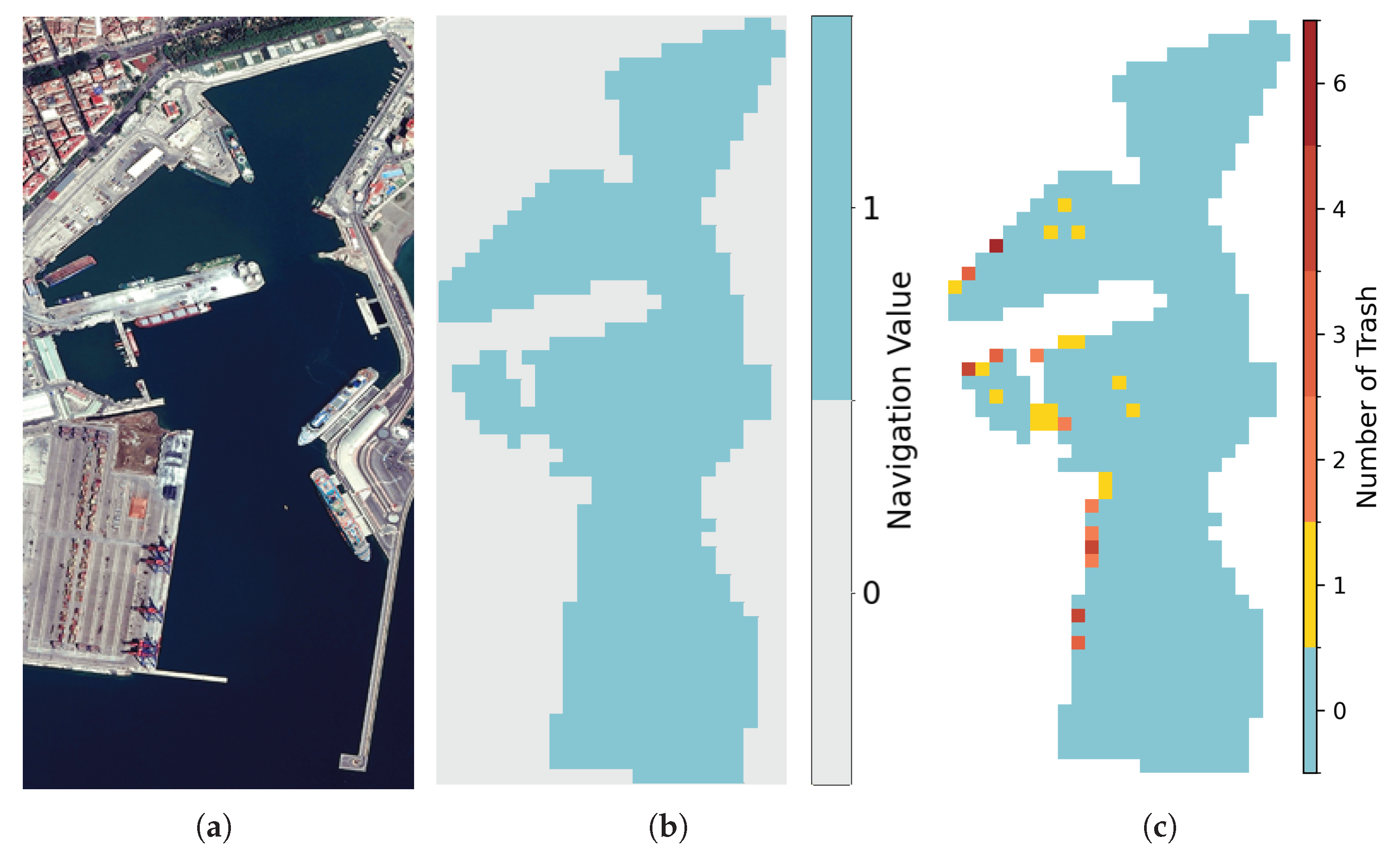
Figure 2.
Illustration of the perception areas for two vehicles (A and B) in a discretized environment with a vision radius . The function represents the number of agents covering each cell, while indicates the number of trash items located within that cell after discretization.
Figure 2.
Illustration of the perception areas for two vehicles (A and B) in a discretized environment with a vision radius . The function represents the number of agents covering each cell, while indicates the number of trash items located within that cell after discretization.
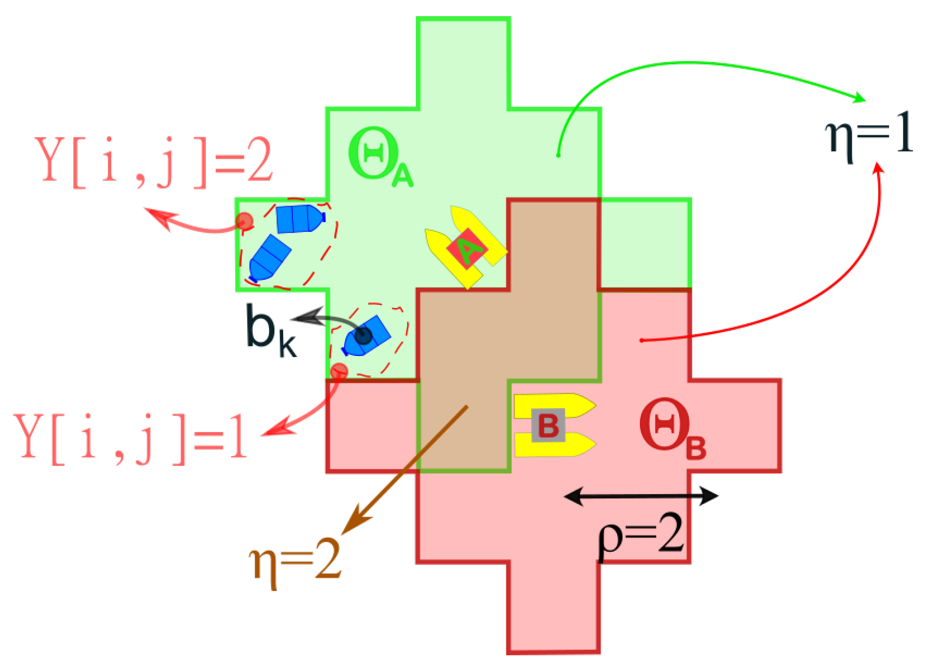
Figure 3.
Diagram of the proposed algorithm. At each step, the environment provides an observation, and all possible task combinations (corresponding to different configurations) are simulated across the fleet. The resulting rewards are computed and scalarized according to user-defined preferences. The Reward-Greedy Policy Selection mechanism then identifies the task combination yielding the highest reward. The selected actions are executed, and the environment advances to produce the next observation.
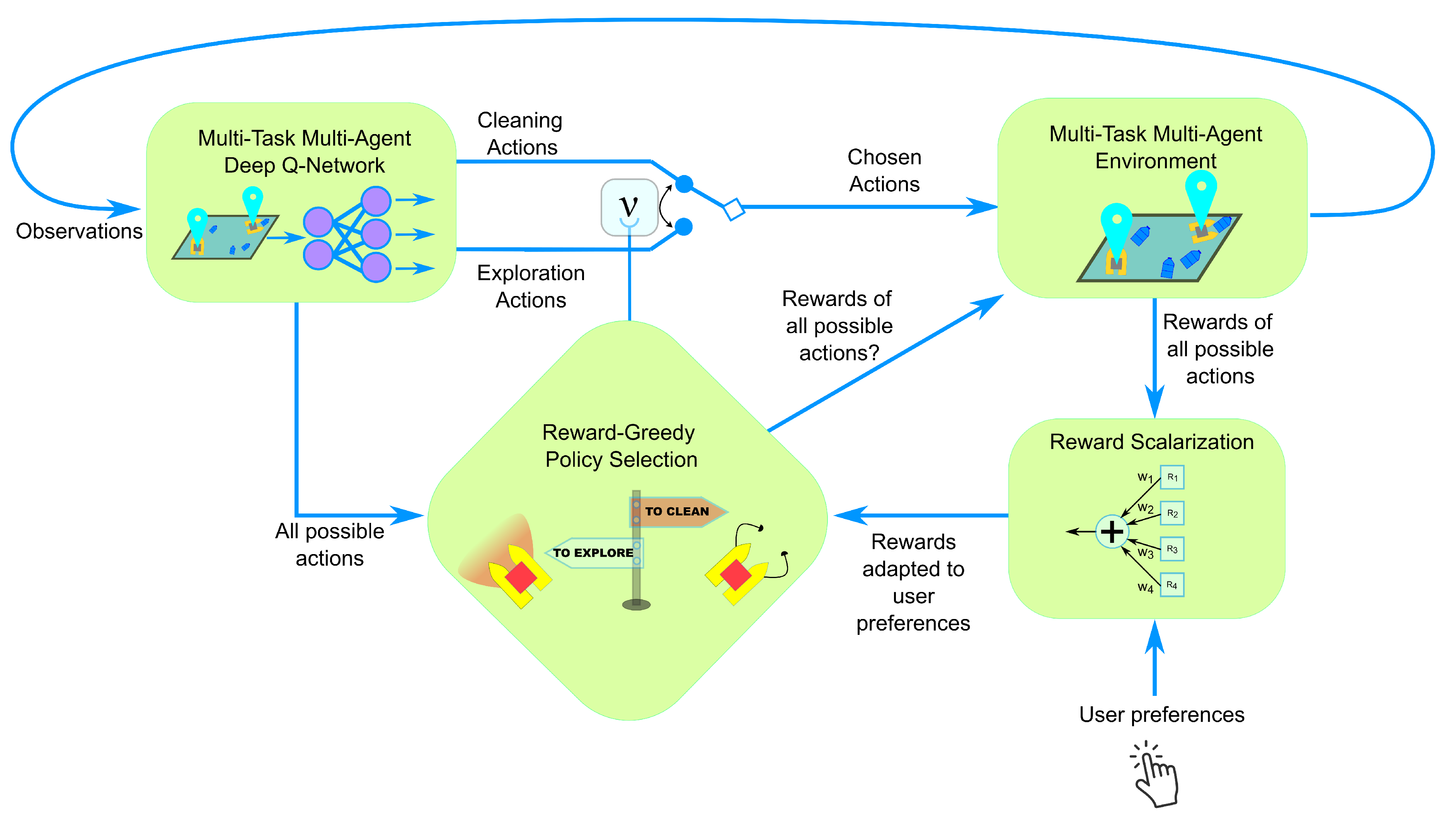
Figure 4.
Results of the scalarization methods. (a) Pareto fronts obtained using each scalarization method across 100 different weight configurations, along with the resulting combined Pareto front that aggregates all non-dominated solutions. (b) Contribution of each scalarization method to the combined Pareto front.
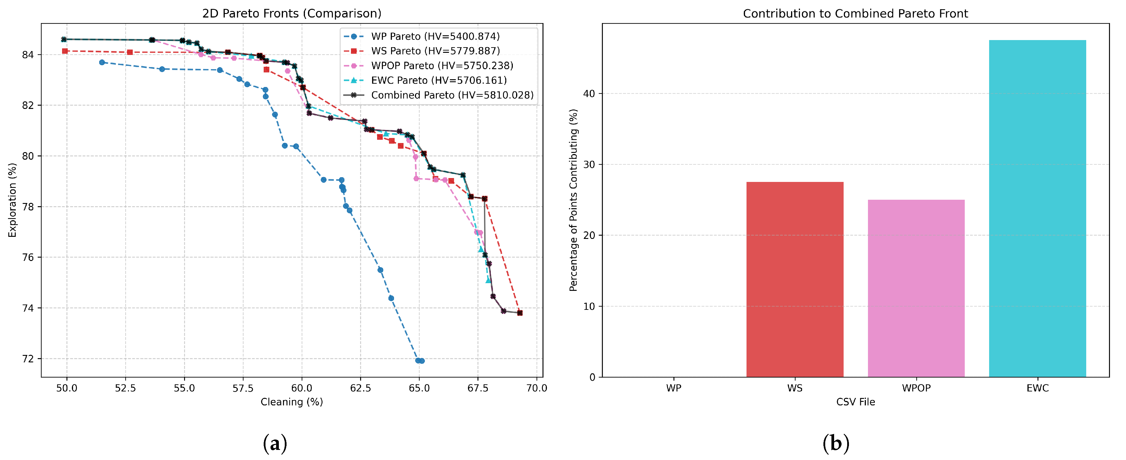
Figure 5.
Illustration of the combined pareto front and the FP2S pareto front.
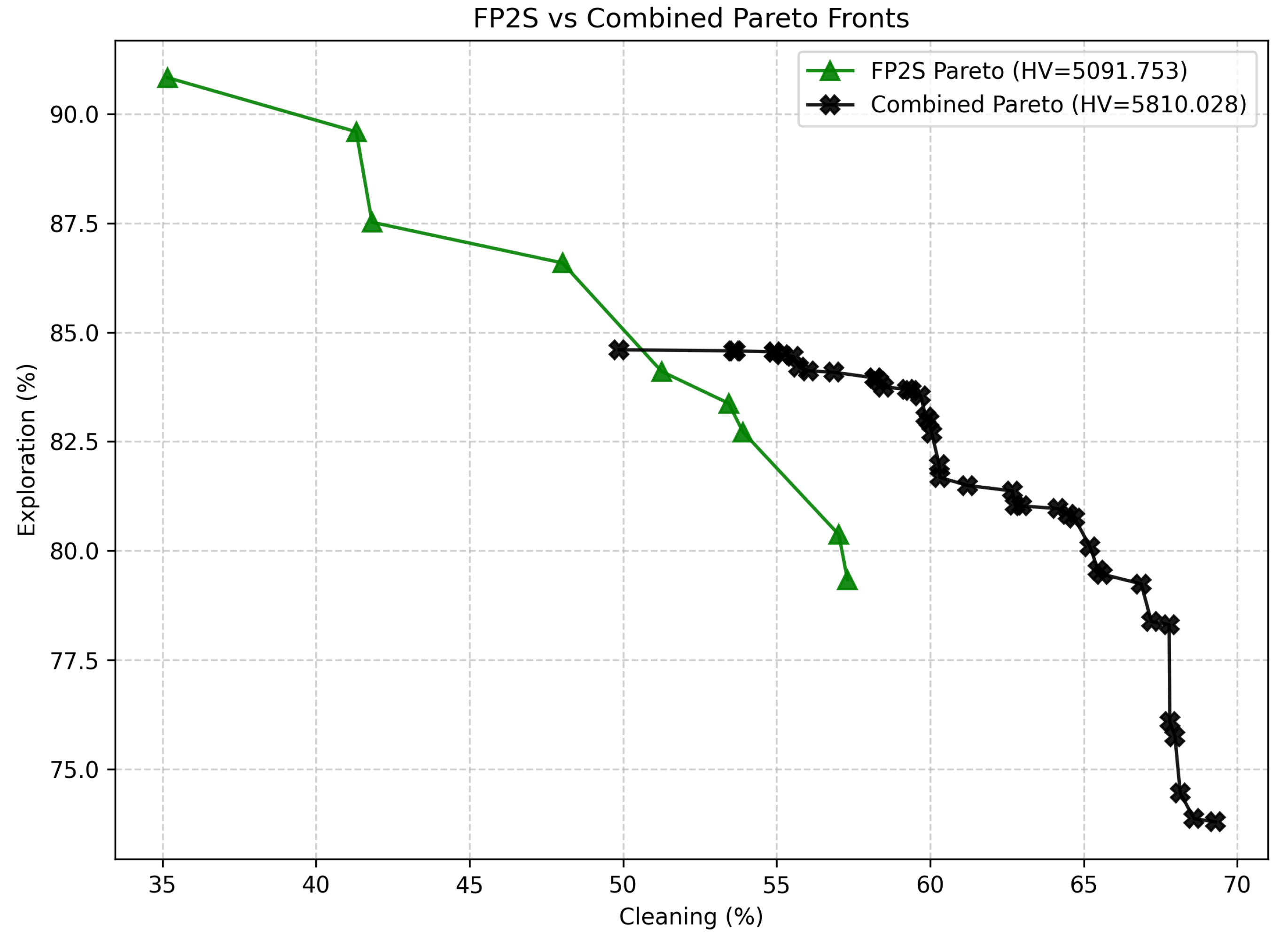
Figure 6.
Evolution of (task allocation) for each of the four agents across a single representative episode under different scalarization methods and weighting preferences, including an FP2S example. Each subplot shows instantaneous task selections. (a) EWC (, ) prioritizes cleaning, (b) WPOP (, ) balances both objectives, (c) WS (, ) emphasizes exploration, and (d) example of FP2S with , illustrating its characteristic switching pattern. All weight values correspond to Pareto-optimal solutions from the combined front.
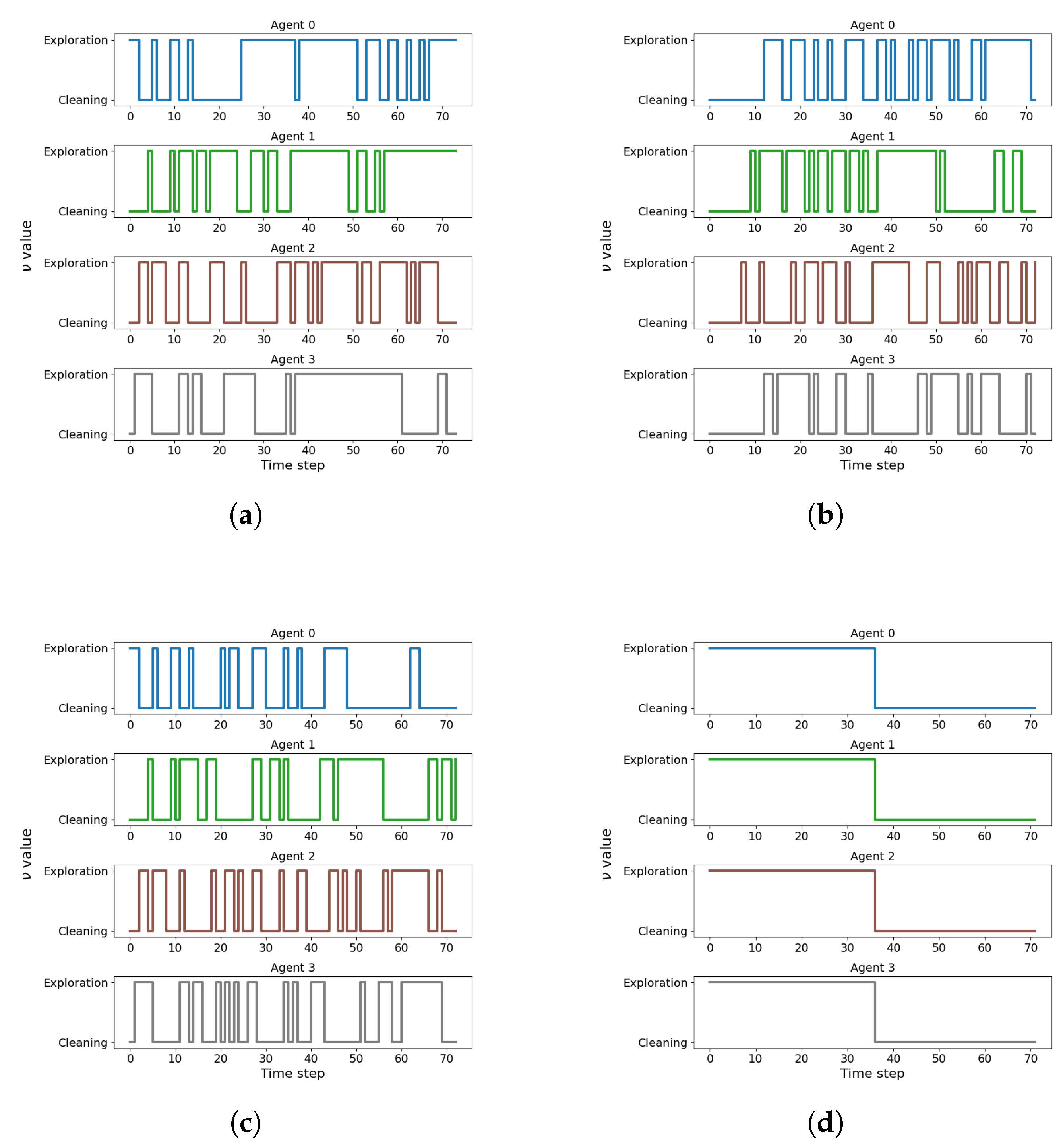

Table 1.
Environment parameters
| Parameters | Values |
|---|---|
| Number of ASVs (N) | 4 |
| Detection radius () | 2 nodes |
| Distance budget | 200 units |
| Movement length | 1 node |
Table 2.
Summary of Pareto front quality metrics for each reward scalarization and the combined front.
Table 2.
Summary of Pareto front quality metrics for each reward scalarization and the combined front.
| Scalarization | Hypervolume | M3 | Spacing | Nº of Points |
|---|---|---|---|---|
| WP | 5400.8738 | 5.0406 | 0.9193 | 21 |
| WS | 5779.8875 | 5.4511 | 1.4368 | 19 |
| WPOP | 5750.2380 | 5.0639 | 0.6876 | 21 |
| EWC | 5706.1609 | 5.2529 | 1.0877 | 23 |
| Combined | 5810.0283 | 5.4977 | 0.7035 | 40 |
| Literature | 5091.7528 | 5.7991 | 2.1422 | 9 |
Table 3.
Wilcoxon signed-rank test results between Pareto fronts for each reward configuration. Significant () differences are highlighted in bold.
Table 3.
Wilcoxon signed-rank test results between Pareto fronts for each reward configuration. Significant () differences are highlighted in bold.
| Comparison | Cleaning (p-value) | Exploration (p-value) |
|---|---|---|
| WP vs WS | 0.2753 | 0.0955 |
| WP vs WPOP | 0.0239 | 0.5392 |
| WP vs EWC | 0.6578 | 0.0022 |
| WS vs WPOP | 0.2935 | 0.1956 |
| WS vs EWC | 0.3321 | 0.1956 |
| WPOP vs EWC | 0.1111 | 0.1193 |
Table 4.
FP2S candidate Pareto-optimal policies evaluated over 200 episodes. The policy labels follow the notation Policy (Type @ PDS), where Type policies, and PDS denotes the fixed exploration duration (e.g., 0.7 represents a mission with 70% exploration time followed by cleaning).
Table 4.
FP2S candidate Pareto-optimal policies evaluated over 200 episodes. The policy labels follow the notation Policy (Type @ PDS), where Type policies, and PDS denotes the fixed exploration duration (e.g., 0.7 represents a mission with 70% exploration time followed by cleaning).
| Policy (Type @ PDS) | Cleaning (%) | Exploration (%) |
|---|---|---|
| Best Exploration @ 1.0 | 35.2 | 90.8 |
| Best Exploration @ 0.9 | 41.3 | 89.6 |
| Best Cleaning @ 0.9 | 41.8 | 87.5 |
| Best Exploration @ 0.8 | 48.0 | 86.6 |
| Best Exploration @ 0.7 | 51.3 | 84.1 |
| Best Cleaning @ 0.7 | 53.4 | 83.4 |
| Final Trained @ 0.7 | 53.9 | 82.7 |
| Best Exploration @ 0.6 | 57.0 | 80.4 |
| Best Cleaning @ 0.6 | 57.3 | 79.3 |
Disclaimer/Publisher’s Note: The statements, opinions and data contained in all publications are solely those of the individual author(s) and contributor(s) and not of MDPI and/or the editor(s). MDPI and/or the editor(s) disclaim responsibility for any injury to people or property resulting from any ideas, methods, instructions or products referred to in the content. |
© 2025 by the authors. Licensee MDPI, Basel, Switzerland. This article is an open access article distributed under the terms and conditions of the Creative Commons Attribution (CC BY) license (http://creativecommons.org/licenses/by/4.0/).
Copyright: This open access article is published under a Creative Commons CC BY 4.0 license, which permit the free download, distribution, and reuse, provided that the author and preprint are cited in any reuse.


