Submitted:
19 November 2025
Posted:
20 November 2025
You are already at the latest version
Abstract
I investigate strategies for semantic decoding from minimal-channel, consumer-grade EEG systems. Using only four electrodes and 50–100 word stimuli, I evaluate convolutional architectures on two semantic tasks including emotional valence and part-of-speech discrimination (specifically, noun/verb classification). To address limited data, I introduce (1) a data amplification method based on short-time FFT snapshots and (2) an embedding-constrained EEG architecture that leverages clustered word embeddings to design specialized processing branches without requiring embeddings at inference. Spectral (FFT) data improved accuracy by~8% over time-series models, while the embedding-constrained architecture reached ~93.5%, outperforming baselines and multi-head models.
Keywords:
EEG
; FFT
; EEGNet
; word embeddings
; embedding-constrained architecture
; brain–computer interface
; semantic decoding
I. Introduction
Decoding semantic information from non-invasive electroencephalography (EEG) is a sought after goal, especially for NLP applications, with applications for brain–computer interfaces (BCIs), cognitive neuroscience, and areas of neurotechnology (Hollenstein N, Renggli C, Glaus B, Barrett M, Troendle M, Langer N et al. Decoding EEG Brain Activity for Multi-Modal Natural Language Processing). Recent convolutional neural network (CNN) approaches (e.g., EEGNet-style architectures) have demonstrated the ability to classify mental states and categories from relatively small EEG datasets by encoding biases into compact models (Lawhern, V. J., Solon, A. J., Waytowich, N. R., Gordon, S. M., Hung, C. P. et. al. (2018). EEGNet: A compact...). However, most prior work relies on multi-channel, research-grade EEG devices with many trials per condition, all of which limit the practicality of the models.
Two practical constraints motivate this experiment. First, consumer EEG devices (here, OpenBCI Ganglion and an associated headband) often provide only a handful of channels. Developing reliable decoders for minimal-channel recordings is essential for low-cost, real-world systems (Maskeliunas R, Damasevicius R, Martisius I, Vasiljevas M. Consumer-grade EEG devices: are they usable for control tasks?). Second, many uses require strong performance from very limited data (tens of stimulus presentations) so methods that utilize information content without collecting more raw trials are valuable.
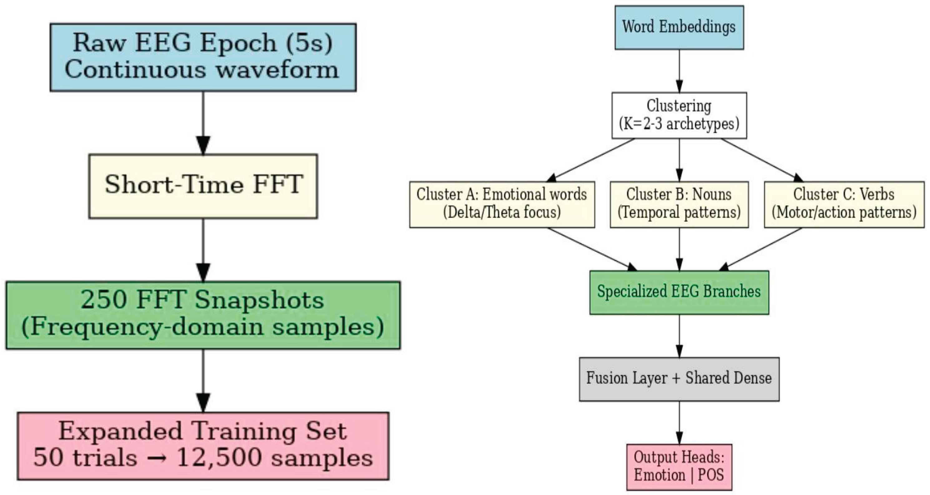
I investigate two strategies to address these constraints. The first is a frequency-domain data amplification approach: by capturing FFT representations and sampling many FFT “plots” per epoch, one can obtain many more training samples from few trials while preserving key spectral signatures of cognitive processing (see Appendix B: Flowchart 2). The second is a linguistically informed architectural approach. Rather than feeding word embeddings into the model at inference (which can cause overfitting and dependence), I use embeddings only during architecture design. I call this the Embedding-Constrained EEG Architecture.
In addition to these two strategies, I evaluated standard baselines: time-series trained EEGNet-style models, LIME- and weight-based explainability to inform channel reweighting, a fused multi-head model constructed from fine-tuned single-task existing models, and an alternative regularizer strategy that attempts to force EEG features toward embedding predictions. I compare performance on two semantic decoding tasks commonly used in EEG studies: emotional valence classification (negative / neutral / positive) and part-of-speech (POS) discrimination (in this case, noun vs. verb) (Gkintoni E, Aroutzidis A, Antonopoulou H, Halkiopoulos C. From Neural Networks to Emotional Networks: A Systematic Review of EEG…). Importantly, I evaluate under strict constraints (four channels and as few as 50 trials per stimulus).
The core hypotheses were: (1) FFT-based sampling will substantially improve classifier performance relative to raw time-series training by carefully increasing effective sample size and making spectral features clear (2) embedding-constrained architectural design will outperform embedding-as-regularizer approaches and even single-task baseline EEGNet-style models by incorporating relevant inductive biases and (3) While channel reweighting will further boost single-participant accuracy by reducing artifactual influence on learned filters, leveraging embeddings will allow a simpler, quicker process to similar accuracies. See Appendix B: Flowchart 1 for a visualization of these processes and hypotheses.
II. Methods
A. Participants
- Number & demographics: For single-participant / participant-level analyses I report results per subject. Similar to Sun et. al. and Wandelt et. al., few participants were used (n=2) (due to focus on single participant decoding) and most models were trained on both datasets independently (evaluation metrics were averaged) (.
- Note: Cross participant evaluations were not tested yet this should be an area of future research. From a practical standpoint however, these models can be easily trained and fine-tuned to individual participants.
B. Hardware & Acquisition
- EEG hardware: OpenBCI Ganglion (and an OpenBCI flat & comb electrodes). Four active channels were used and optimized for semantic decoding (schematic provided in Figure 1). For both tasks, electrodes were placed at TP7, TP8, F7, and F8 in accordance with the universal 10-20 system (see Figure 1) (Maskeliunas R, Damasevicius R, Martisius I, Vasiljevas M. Consumer-grade EEG devices: are they usable for control tasks?). For sampling, LSL (lab streaming layer) was used to stream data from the OpenBCI GUI.
- Sampling rate: Sampling rate was 200 Hz over 5-second epochs (1000 points/sample), with both time-series and FFT data (60 bins, 250 snapshots) collected per trial.”
C. Impedance & Quality Control: Channels Checked Before Each Session; Trials with High Impedance Levels Were Ignored
D. Stimulus Presentation: Words Displayed Centrally on a Monitor with a Fixation Cross Between Trials. Timing: Stimulus Duration = 5 s, Inter-Stimulus Interval ~ 1-2 s.
E. Stimuli & Experimental Design
- Word lists: Two primary semantic tasks: emotional valence (words labeled negative / neutral / positive) and part-of-speech (noun vs. verb). Experiments described in the introduction used sets of 50 unique words (each).
- Trial structure: Each word was presented for each trial; participants were asked to ponder the word (in addition to passive viewing). Each word had 0 repetitions
- Total trials & augmentation rationale: For the FFT-based method I treated every other FFT “window” or “snapshot” from a single epoch as separate training samples (see Feature Extraction). For example, 50 words × 125 FFT samples per word → 6250 FFT samples; with 100 words → 12500 FFT samples.
F. EEG Preprocessing
All preprocessing steps were implemented through a custom NumPy, TensorFlow, Scikit-learn pipeline. The exact script is provided in the repository (to be released soon).
Note: Bandpass filtering & line-noise removal are done automatically by streaming the “timeseriesfilt” data from the LSL. This applies these filters automatically.
- Bandpass filtering: 0.5–100 Hz
- Line-noise removal: notch filter at 50/60 Hz
- Normalization: Percentile-based scaling: for each channel, values were normalized using the 5th–95th percentile range to reduce the influence of extreme values. This approach improves strength across sessions/participants and is used prior to data entrance into the model.
G. Feature Extraction & FFT Sampling
I compared two primary feature representations.
-
Raw time-series
- The epoch time-series (shape: channels, timepoints) after preprocessing was used directly as input to time-domain CNN architectures. For the EEGNet-style baseline the input tensor shape was (channels, timepoints, 1). Note: An extra dimension was added for compatibility with the EEGNet inspired architecture.
-
FFT-based frequency-domain sampling (data amplification trick; see Appendix B: Flowchart 2)
- Rationale: FFT representations can expose certain features (delta/theta/alpha/beta/gamma bands). Because 250 “snapshots” of this FFT data occurred over a different time interval (~2 seconds) I can treat each FFT “plot” as its own sample. In this case, every other snapshot was treated as a unique training sample with the same label as the parent sample (leaving 125 unique samples per trial). Important: It was ensured that trial-level splits were implemented to prevent data-leakage.
-
Parameters used:
- Frequency bins: 1–60 Hz
- Number of snapshots per sample: 125
- Normalization: Each FFT snapshot was normalized using the same percentile scaling as for the time-series.
- Representation: For CNNs I formatted each FFT snapshot as a 2D “shape” (channels × frequency bins) so that depthwise/separable convolutions could learn spatial-frequency filters.
Note: The input to the EEG CNN is 3 dimensions as in the case of the time-series data. However, when collecting 50 trials of FFT data the resulting shape is 4 dimensions: (50, 250, 4, 60). As noted above, I treated every other FFT sample as its own sample to increase the data size from a few trials which resulted in the shape (6250, 4, 60) (this is now compatible with the CNN). Other efforts were explored including taking the mean of all 250 samples to produce the shape (50, 4,60), yet as expected, this yielded poor results in comparison to the larger dataset (see Appendix B: CM 1)
H. Model Architectures & Development Pipeline (see Appendix A for Detailed Architectures)
I developed the modeling strategy iteratively. Starting from an EEGNet-style baseline trained on time-domain epochs, I moved to spectral inputs (FFT snapshots) to amplify effective sample size and expose frequency features. Explainability via LIME and early-layer weight inspection then guided multiplicative channel reweighting and fine-tuning (all of which reduced artifacts/noise). To efficiently reuse trained models across tasks I built a fused multi-head model that concatenates early weights and uses task-specific heads. Finally, leveraging word-embedding clusters to add biases, I designed the Embedding-Constrained architecture consisting of cluster-specific branches (e.g. emotion-focused low-frequency branch; sensory-focused high-frequency branch). An alternative strategy that enforced embedding prediction as an “auxiliary regularizer” was evaluated but found to show unstable optimization, over dependencies, and poor accuracies. Hence I focus on the embedding-constrained approach as the primary model4.
-
EEGNet-style baseline
- Based on the EEGNet design1 (compact model with multiple filters)
- Key layers: Depthwise spatial filter (per-channel) and separable convolution (to capture temporal patterns).
-
Explainability & LIME-guided channel reweighting
- After training EEGNet-style models, I extracted early-layer filter weights and used LIME (Local Interpretable Model-agnostic Explanations) to estimate channel contributions to predictions (and to discern artifacts/noise)
- Channels were then weighted accordingly via multiplicative channel scaling in the input
-
Fused multi-head model (fine-tuning fusion)
- Individual single-task models (emotion, POS) were trained together to demonstrate the efficacy of a fusion model. Early convolutional weights were extracted and concatenated into a fused encoder, and task-specific heads were attached.
- Embedding-Constrained EEG Architecture (primary proposed model)
Design pipeline (see results, F and Appendix A: Table A1, A2, A3 for more information on the model specifics)
- Generate word embeddings using OpenAI’s text-embedding-3-small for the full stimulus set (n = 100 words) (He T, Boudewyn MA, Kiat JE, Sagae K, Luck SJ. Neural correlates of word representation vectors in natural language processing models…)
- Cluster embeddings into K semantic archetypes (K manually chosen; in the experiments K = 2). Archetypes include groups like emotional, concrete/sensory, abstract, noun/verb etc
- Clustering group categories are determined by evaluating embeddings for words closest to the centroid (and then used as representations for the cluster as a whole)
- For each grouping I created a specialized processing branch with convolutional filters tuned to frequency bands expected for that archetype (neuroscience-informed choices: emotion → emphasis on delta/theta/alpha; noun/verb → include beta/gamma etc) (Pulvermuller F, Preissl H, Lutzenberger W, Birbaumer N. Brain rhythms of language: nouns versus verbs),(Gkintoni E, Aroutzidis A, Antonopoulou H, Halkiopoulos C. From Neural Networks to Emotional Networks: A Systematic Review of EEG...). Specifically, temporal convolution sizes and filter sizes are then utilized that bias each branch to the target frequency bands (see Table A1, A2, A3 for detailed architecture).
-
Each branch processes FFT input (channels × frequency bins). Branch outputs are concatenated and passed to shared dense layers, and then to task-specific heads.
- Key property: embeddings are used only for architecture construction, not at inference. In this way, the model is forced to learn EEG related patterns and not over-rely on embedding information (it was demonstrated that the model often prioritizes the embeddings over the noisy EEG data when embeddings were involved in training).
- 5.
-
Embedding-as-regularizer (alternative strategy)
- Includes an auxiliary loss (extra loss function) forcing learned EEG embeddings to correlate with word embeddings (i.e, cosine similarity). The goal was to create a joint-embedding space that represented both EEG data and word embeddings. I found this strategy often caused optimization conflicts, over-reliance on the embeddings and poorer performance. Nevertheless, it was implemented for comparison and to explore alternate uses of word embeddings.
I. Loss Functions & Optimization
-
Primary loss: Categorical cross-entropy with focal loss (gamma=1.5, alpha=0.25) for imbalanced emotion classes (20 pos/15 neu/15 neg); POS was balanced.
- For FFT data, trial level split was implemented to ensure integrity.
- Optimizer: Adam with initial learning rate = 1e−3 for training from scratch; 1e−4 for fine-tuning fused models.
- Regularization: Dropout in dense layers (e.g., 0.4).
- Batch size: (example) 32 for FFT snapshots, and smaller (16) for time-series
- Epochs & early stopping: maximum epochs = 100 with early stopping based on validation loss/patience = 20 epochs.
J. Training & Evaluation Protocol
- Data splits: Performing train/validation/test splits, Stratified Shuffle Split was utilized: n_splits = 1, random state = 42, test size = 0.2
- Within-participant fine-tuning: For fused and embedding-constrained experiments, I report both (a) models trained from scratch per participant and (b) models built via transfer/fine-tuning from other participants’ weights (to simulate realistic use where a pretrained model is personalized).
K. Evaluation Metrics & Statistical Tests
- Primary metric: classification accuracy. Baseline chance levels: emotion (3-class) = 33.3%, POS (2-class) = 50%.
- Secondary metrics: confusion matrices, LIME analysis, and convolutional weight visualizations where applicable.
- Evaluations: Model accuracies were evaluated by, after training the model, shuffling the validation/testing set, randomly sampling 40-80%, evaluating the accuracy and repeating 100 times. The accuracies were then averaged to ensure it represented the models true performance. Classification accuracies are reported with 95% Wilson binomial confidence intervals, computed relative to the number of test trials.
L. Explainability & Weight Analysis
- Weight visualization: plot early convolution (depthwise & separable) filters and their spatial maps to inspect learned spatial & temporal patterns.
- LIME: applied to trained EEGNet-style models to estimate per-channel/frequency contributions to single-sample predictions. LIME outputs guided channel reweighting: channels consistently identified as artifactual or noisy were downweighted (by a multiplicative scalar) and models fine-tuned. Results of reweighting are reported.
- Other studies: evaluating performance after removing reweighting, removing/adding noise, etc.
M. Reproducibility & Code/Data Availability
- Code: all preprocessing, model definitions, training scripts, and analysis notebooks are available in the project repository (to be provided). Versions of libraries (TensorFlow, NumPy, etc.) will be included.
- Data: raw EEG data will be shared via the same repository in a pkl file. FFT snapshots and model weights will not be provided explicitly but the code to extract such weights will be available.
III. Results
A. Data Quantity, Preprocessing, and Effective Sample Amplification
Across experiments I evaluated two main stimulus set sizes: the 50-word condition used for the single-task experiments and a 100-word combined set on the embedding model. FFT sampling yielded ~6,250 (50-word) or ~12,500 (100-word) samples per dataset.
B. Preprocessing Outcomes and Channel Quality
Percentile-based normalization produced stable per-channel scales across sessions including on the 5th-95th percentile (see Methods). LIME and depthwise & separable weight inspection identified one or two channels with consistent low contributions that were subsequently down-weighted in the reweighting experiments (see below).
C. Representation Comparison: Time-Series vs FFT Snapshots
To determine whether frequency-domain or fast fourier transform sampling (FFT) improves classifier performance relative to raw time-series input, I trained identical EEGNet-style architectures on (a) preprocessed time-domain epochs and (b) FFT snapshots derived from the exact same trials (data amplification was conducted for FFT samples as discussed in Methods). Both models are single-task models without custom layers or adaptations.
It was concluded that FFT-trained models significantly outperformed time-series models for both emotion and POS tasks, indicating that FFT data both (a) expose features and (b) allow for increasing training sample size, which in turn, is shown to benefit model performance (see Figure 2). Specifically, FFT models outperformed time-series by ~8% on emotion and ~4% on POS (Figure. 2; see Appendix B: CM 2 for POS). All the models in Figure 2 consisted of the original architecture outlined in Appendix A: Table A4.
D. Explainability, Channel Reweighting, and Single-Participant Fine-Tuning
To identify channel/frequency contributions and reduce artifactual/noise influence in the baseline time-series model, I applied LIME and early-layer weight visualization, and tested multiplicative channel reweighting followed by re-training on the baseline time-series model evaluated in Figure 2. LIME indicated that channels 1 and 2 contributed most to emotion discrimination, and were therefore not modified with weights. After weight visualization, Channels 3 showed artifact-like signatures (e.g. spikes including EMG likely from eye movements hence the symmetric oscillations) and were then used for down-weighting (see Figure 3). Figure 4 graphs the influence of individual channels from the LIME analysis. I applied multipliers w (0 < w ≤ 1) to channels with artifacts or heavy negative influence (channels 3 and 4) then retrained the model (see Methods).
Scalars, w, were applied to solely the training data on channels with artifacts or large negative influence. In doing so, I guide the model in learning relevant patterns and steering away from relying on noise. Many weights were experimented with (see Appendix B: CM 1), but the weights [1, 1, 0.6, 0.6] resulted in the highest accuracy and an increase from the unweighted model (see Figure 5). Weights were applied to channels 1 (TP7) , 2 (TP8) , 3 (F7), and 4 (F8) respectively.
The new learned features and weights were analyzed. This was done in the same manner using LIME analysis. Figure 6 displays the average contribution per channel of the newly weighted model. The newly weighted model no longer depended on artifacts in channel 3 (chan. 2 on figure). With this, the model began to utilize channel 2 (chan. 1 on figure) to a greater degree which was rich in patterns.
Through extensive weight analysis and subsequent reweighting, accuracies can be significantly improved. This same pipeline was utilized in noun/verb classification in which the same trends arose (see Appendix B: CM 3 and Analysis 1 for more details). While this may be plausible it is often tedious, time consuming and resource intensive. In Figure 7 I demonstrate the innate ability of FFT models to more efficiently and accurately rely on correct channels across both emotion and POS tasks (see Figure 7; Appendix B: Analysis 1) The FFT model clearly has correctly relied less on channels 3 and 4 (2 and 3 on the figure). This FFT model accuracy exceeded that of the baseline time-series model by ~9% and the weighted time-series model by ~6%.
E. Fused Multi-Head Model (Fine-Tuning Fusion)
To create an efficient multi-task model without retraining from scratch, using existing FFT models (due to its efficacy demonstrated above), I fused early convolutional encoders from these independently trained single-task FFT models and fine-tuned shared dense layers plus task-specific heads (see methods). The models evaluated in the following figures used early learned weights from the emotion and POS single-task models. These were then concatenated into a fused encoder. In Figure 8, the fused model (see Appendix A: Table A5 for architecture) underperformed single-task models (~16% worse on emotion, ~9% on POS; Figure 8). LIME showed artifact reliance (Figure 9), and reweighting yielded negligible gains (~0.3%; Figure 10 and Figure 11).
Fusing early encoders allows for the reuse of learned spectral and spatial filters, and reduces training cost and resource use. The weighted, fused model offered a modest improvement in combined multi-task accuracy while only some decline in per-task performance. However, the futility of reweighting causes a problem in optimizing and boosting accuracies of these types of models. Hence, a new approach to multi-task classification will be explored in the following section.
F. Embedding-Constrained EEG Architecture (Proposed Model; see Appendix B: Flowchart 2)
To test whether linguistic structure can inform architecture design, I clustered word embeddings into semantic groups and built specialized branches per group (embeddings were not used at inference).
Architecture summary (see Appendix B: Flowchart 2): K = 2 clusters (method = KMeans, embeddings = OpenAI’s text-embedding-3-small). Branches: dynamically adjusted based on clustering results (See Methods & Appendix A: Table A1 for more details.)
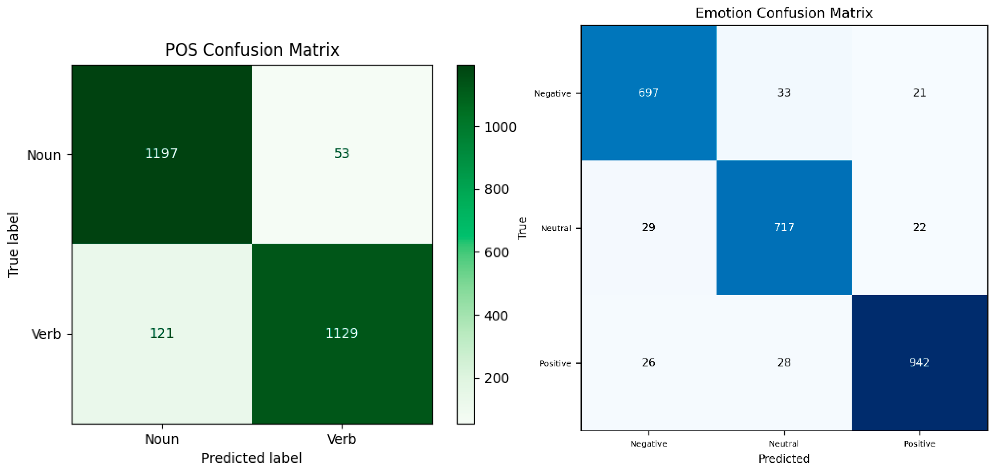
The embedding-constrained model was trained from scratch using FFT data from both emotion and POS tasks (see Results, C), processing EEG inputs in parallel via specialized branches derived from embedding clusters (e.g., emotion, concrete/abstract, noun/verb), each with neuroscience inspired filters tuned to relevant frequencies. Branch outputs are concatenated into a shared layer, enabling the model to learn branch weighting for final classification. With embeddings, it dynamically analyzes stimulus words, leveraging semantic representations5, to build these branches, though currently manually designed (automatable via OpenAI API). This architecture significantly outperformed baselines and fused models, and matched single-task emotion performance (see Figure 12). It was ~4% better than single-task POS, and ~12.5% better overall than the best multi-head fusion.
G. Embedding-as-Regularizer Strategy (Alternative)
To contrast with architecture-level embedding usage, I implemented an auxiliary embedding-prediction loss (cosine similarity) to force EEG features toward semantic vectors and evaluated its performance relative to the proposed model. I hypothesized that a loss forcing the model to learn vectors would compete with the EEG loss, resulting in lower accuracies and less learned EEG patterns (and hence an overreliance on embeddings).
This approach dropped accuracy ~20-30% and caused instability/overfitting, supporting architecture-level biases over auxiliary losses.
H. Summary of Mean Test Accuracies over 100 Shuffled Evaluations (Accuracies Are Reported with 95% Wilson Binomial Confidence Intervals; Note: For Time-Series Models, CI Will Be Large Due to Small Testing Sizes but This Is Mitigated Through Shuffling and Averaging for Confidence (see Methods)
| Model / Representation | Emotion acc (%) mean | POS acc (%) mean | Combined, mean acc (%) | Task Count |
| Time-series EEGNet | 87.50% 95% CI: 46.48 – 98.26 |
89.74% 95% Cl: 48.9 - 98.83 |
88.62% | Single-task |
| FFT-EEGNet | 95.77% 95% CI: 94.94 – 96.43 |
93.94% 95% CI: 92.57 – 95.06 |
94.86% | Single-task |
| Time Series + LIME reweight | 90.12% 95% CI: 61.74 – 98.05 |
- | 90.12% | Single-task |
| Fused multi-head (with best weights) | 74.70% 95% CI: 73.59 – 75.72 |
80.6% 95% CI: 79.23 – 81.8 |
77.65% | Multi-task |
| Embedding-constrained | 94.12% 95% CI: 93.42 – 94.96 |
93.04% 95% CI: 92.16 – 93.83 |
93.58% | Multi-task |
| Embedding-regularizer | 64.95% 95% CI: 63.21 – 66.35 |
73.82% 95% CI: 72.53 – 75.42 |
69.39% | Multi-task |
IV. Discussion
I introduced and analyzed strategies for semantic decoding from minimal EEG: (1) FFT data amplification from short FFT snapshots, (2) channel reweighting, (3) fusion for multi-task classification, and (4) an embedding-constrained EEG architecture using word embeddings just during design. Under constraints of four channels and 50–100 stimulus words, this model achieved the strongest performance across emotional valence (negative/neutral/positive) and part-of-speech (noun/verb) tasks. FFT-trained models consistently outperformed time-series baselines, highlighting spectral data’s efficacy in data-limited scenarios (see Results and Table 1).
The embedding-constrained gains come from encoding neuroscientifically informed biases into network structure, with specialized branches tuned to certain frequency bands (e.g., delta/theta/alpha for emotion; beta/gamma for noun/verb2. This builds on current optimization techniques for EEG architectures4. In contrast, the “embedding-as-regularizer” approach showed poor accuracy due to optimization conflicts in noisy data, underscoring the advantages of simpler biases over multiple losses. EEGNet’s design allowed for an explainability pipeline (depthwise/separable filter inspection + LIME) that identified artifactual channels and guided reweighting for accuracy improvements.
Several limitations deserved highlighting. First, lacking cross participant testing limits inference strength. Second, consumer EEG hardware (OpenBCI Ganglion) adds noise, enhancing practicality, but limiting generalizability. Third, FFT amplification risks bias despite precautions. Such precautions were employed here due to small datasets and single-participant focus but should be minimized with larger, more diverse data. Fourth, branch designs depend on embedding models and clustering, potentially causing less ideal architectures (as evidenced by modest POS gains (~2%) versus emotion (~7%)). Finally, high within-participant accuracies need real-time validation.
This work’s implications include pathways to low-cost BCIs for semantic decoding with few channels and trials, leveraging linguistic knowledge (as in EEG-NLP decoding7) for compact architectures, using reweighting for refinement, and applying FFT enlargement when generalization is not a necessity.
Recommended next steps: replicate with diverse groups to assess generalization and fine-tuning. Explore alternate clustering methods and semantic tasks for flexibility. Develop methods for across subject accuracy. Optimize electrode placements and conduct real-time evaluations. Finally, reduce data amplification reliance for larger datasets.
V. Conclusions
FFT sampling generated larger training sets with little expected leakage, showing better performance over time-series inputs. Reweighting provided single-participant gains, while fused multi-head models enabled decent multi-task accuracy. The embedding-constrained architecture delivered strongest accuracies (~93.5%), requiring only EEG at inference and showing strong performance across tasks with quick, resource light training. These findings illustrate how neuroscience informed biases and FFT features can reduce data and hardware demands for semantic BCI’s. Future efforts should expand experimental size, add more specialized pathways, automate cluster analysis, reduce reliance on amplification, and enable real-time decoding.
Funding
This work received no specific grant or financial support from any funding agency, commercial entity, or not-for-profit organization.
Appendix A: Model Architectures

Table A1.
Model Architecture Specifications for proposed embedding-constrained model.
| Component | Layer Type | Purpose |
| Input Layer | Input | EEG signals (4 channels, 60 time points) |
| Specialized Processing Branches | ||
| Emotion Branch | Conv2D | Low-frequency emotional patterns |
| Conv2D | Delta/theta/alpha band focus | |
| MaxPooling2D | Reduce size | |
| BatchNormalization | Normalize | |
| Noun Branch | Conv2D | Capture representation patterns |
| Conv2D | Temporal object processing | |
| MaxPooling2D | Spatial-temporal reduction | |
| BatchNormalization | Normalize | |
| Verb Branch | Conv2D | Motor-action network activation |
| Conv2D | Action planning patterns | |
| MaxPooling2D | Feature compression | |
| BatchNormalization | Normalize | |
| Feature Fusion | ||
| Flatten | Branch output flattening | |
| Concatenate | Multi-branch feature fusion | |
| Dense | Share representation | |
| Shared Processing | ||
| Dense | Feature extraction | |
| BatchNormalization | Training stabilization | |
| Dropout | Overfitting prevention | |
| Dense | Share representation | |
| BatchNormalization | Training stabilization | |
| Dropout | Regularization | |
| Output Heads | ||
| Emotion Classification | Dense | Negative/Neutral/Positive |
| POS Classification | Dense | Noun/Verb |
Table A2.
Training Config. for embedding constrained model.
| Parameter | Value | Description |
| Input Shape | (4, 60, 1) | 4 EEG channels, 60 time points, 1 feature |
| Optimizer | Adam | learning_rate=1e-5 |
| Loss Function | Balanced Focal Loss | α=0.25, γ=1.5 for both tasks |
| Loss Weights | [1.2, 1.0] | Emotion task: 1.2, POS task: 1.0 |
| Batch Size | 32 | Batch |
| Epochs | 100 | Maximum training iterations |
| Validation Split | 20% | Stratified shuffle split |
| Early Stopping | 15 epochs patience | Monitor validation loss |
| Learning Rate Reduction | Factor=0.5, patience=8 | Adaptive learning rate |
| Data Normalization | Robust percentile | 5th-95th percentile inclusion |
Table A3.
Architecture Design Principles.
| Design Principle | Implementation | Neuroscientific Rationale |
| Frequency-Specific Processing | Different kernel sizes per branch | E.g: Emotion: low-freq patterns, Noun: sustained patterns, Verb: dynamic patterns |
| Spatial Attention | Varying spatial filter | Noun: temporal areas, Verb: motor-frontal activation |
| Multi-Task Learning | Shared features but separate heads | Learns from all branches |
| Embedding-Informed Design | Cluster analysis architecture | Word semantics guide neural processing |
| EEG-Only Inference | No text input or embedding input required | Deployable and practical for real-time BCI applications |
Table A4.
Architecture summary for baseline FFT and time-series models (single-task). This architecture mirrors that of EEGNet, using both separable filters and depthwise filters (utilized as it is applied to each channel separately).
Table A4.
Architecture summary for baseline FFT and time-series models (single-task). This architecture mirrors that of EEGNet, using both separable filters and depthwise filters (utilized as it is applied to each channel separately).
| Layer | Type | Purpose |
| Input | Input | Raw EEG or FFT input |
| Temporal Convolution Block | ||
| Conv2D_1 | Conv2D | Temporal filtering across time |
| BN_1 | BatchNormalization | Normalize activations |
| Block 2: Spatial Convolution | ||
| DepthwiseConv2D | DepthwiseConv2D | Spatial filtering across channels |
| BN_2 | BatchNormalization | Normalize activations |
| Activation_1 | ELU | Non-linear activation |
| Pool_1 | AveragePooling2D | Downsample |
| Dropout_1 | Dropout | Regularization |
| Separable Convolution Block | ||
| SeparableConv2D | SeparableConv2D | Efficient feature extraction |
| BN_3 | BatchNormalization | Normalize activations |
| Activation_2 | ELU | Non-linear activation |
| Pool_2 | AveragePooling2D | Further downsampling |
| Dropout_2 | Dropout | Regularization |
| Classification Head | ||
| Flatten | Flatten | Convert to 1D |
| Dense | Dense | Classification output (either emotion or POS) |
Table A5.
Architecture summary for the multi-head fused model. Note, “attention” was implemented to properly and flexibly combine both pre-trained feature vectors. These models were subsequently weighted with the goal of achieving higher accuracies. Shown is the model specs before weighting.
Table A5.
Architecture summary for the multi-head fused model. Note, “attention” was implemented to properly and flexibly combine both pre-trained feature vectors. These models were subsequently weighted with the goal of achieving higher accuracies. Shown is the model specs before weighting.
| Layer | Type | Purpose |
| Input | Input | EEG (FFT) input |
| Feature Extraction | ||
| Emotion_Extractor | Frozen EEGNet | Extract emotion features |
| POS_Extractor | Frozen EEGNet | Extract POS features |
| Emotion_Flatten | Flatten | Flatten emotion features |
| POS_Flatten | Flatten | Flatten POS features |
| Attention Fusion Block | ||
| Emotion_Proj | Dense | Project emotion features |
| POS_Proj | Dense | Project POS features |
| Emotion_Att | Dense | Emotion attention weights |
| POS_Att | Dense | POS attention weights |
| Emotion_weighted | Lambda | Apply attention to emotion |
| POS_weighted | Lambda | Apply attention to POS |
| Fused | Concatenate | Combine weighted features |
| Fusion Processing | ||
| Fusion_Dense1 | Dense | First fusion layer |
| Fusion_BN1 | BatchNormalization | Normalize activations |
| Fusion_Dropout1 | Dropout | Stability |
| Fusion_Dense2 | Dense | Second fusion layer |
| Fusion_BN2 | BatchNormalization | Normalize activations |
| Fusion_Dropout2 | Dropout | Stability |
| Output Heads | ||
| Emotion_Output | Dense | Emotion classification |
| POS_Output | Dense | POS classification |
Appendix B: Extended Results, Graphs, & Confusion Matrices
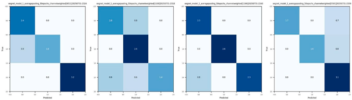
CM 1. (below) An array of the weighted, time-series trained models (with the [1, 1, 0.6, 0.6] weighted model performing the best) and their corresponding confusion matrices.
CM 2. (below) Left to right: (1) Baseline, single-task FFT trained model for noun/verb (POS) classification. Reported mean accuracy of 93.93%. (2) Baseline, single-task time-series model for noun/verb (POS) classification. Reported mean accuracy of 89.74%. FFT models showed an inherent mean accuracy improvement of ~4%.
CM 3. (below) Confusion matrices (CM’s) for another weighted multi-head fused model. The following weights were used: [1, 1, 0.7, 0.8]. Mean accuracies are reported below. A decrease is shown in performance from the previous weighted multi-head model. A slight increase is shown (~2%) in POS classification. Overall, the average performance decreased by about (1-2%) across tasks.
Analysis 1. (below) Left to right: (1) LIME analysis was performed to understand the average channel influence on a POS, FFT-trained baseline model. It’s clear it learned to give negligible influence to artifactual channel 3 (chan. 2 on figure) and correctly prioritize channel 1 (chan. 0 on figure) without weighting (shown to be correlated with higher accuracies). (2) Shown is the same representation of channel influence for a weighted time-series model, attempting to prioritize channels 0 and 3 in POS classification. This model struggled to learn patterns from these channels and likely relied slightly on artifacts resulting in a ~4% decrease in accuracy for POS tasks.
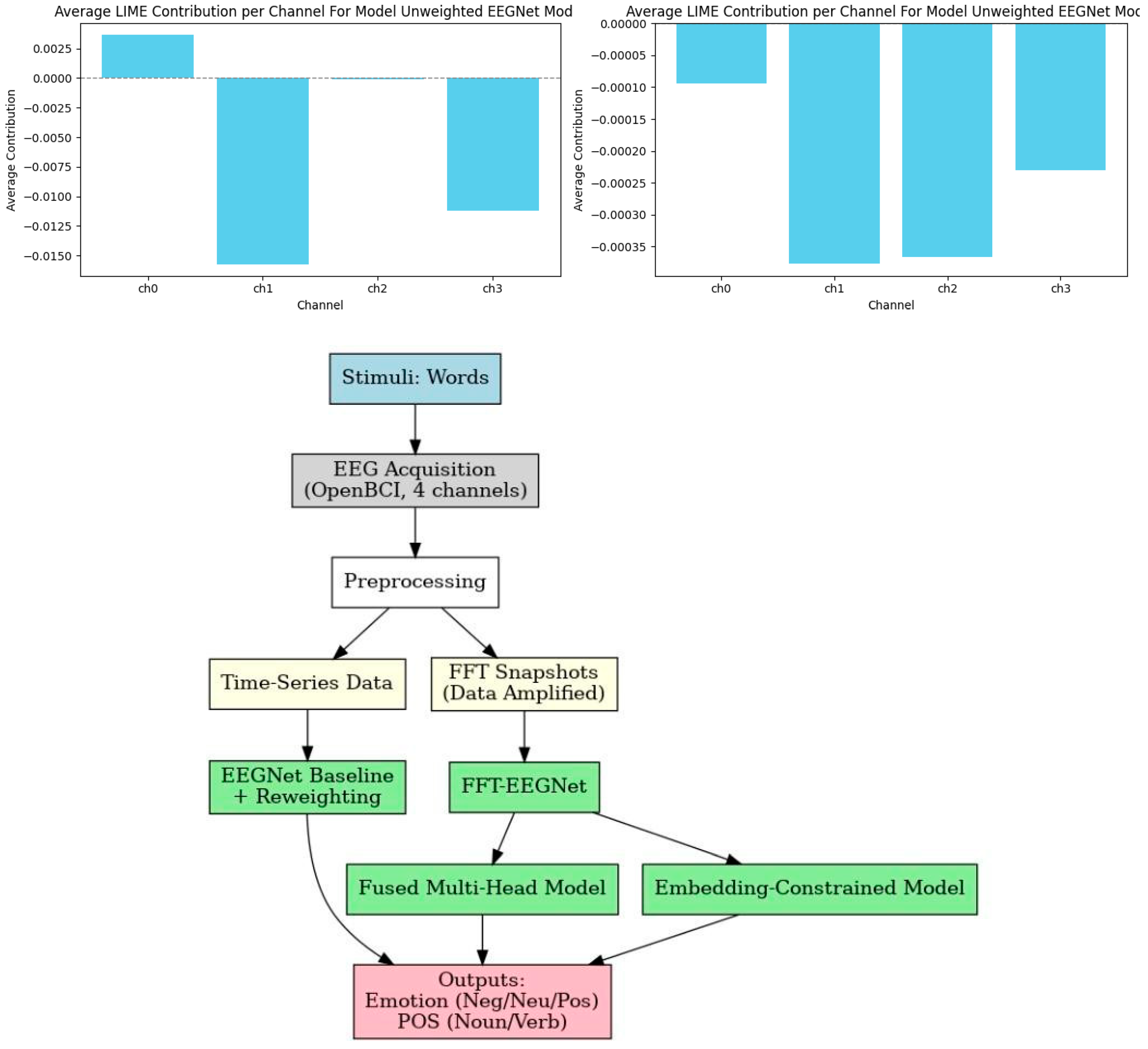
Flowchart 1.
Introduction summary and outline for experiment processes.
Flowchart 2.
Left to right: (1) Visualization of FFT data sampling amplification procedure. (2) Visualization of proposed embedding-constrained model.
Flowchart 2.
Left to right: (1) Visualization of FFT data sampling amplification procedure. (2) Visualization of proposed embedding-constrained model.
Informed Consent Statement
All participants involved in this laboratory exercise provided their consent to participate voluntarily. The experiment posed no physical, ethical, or privacy risks, and all members contributed equally to data collection and analysis.
Data Availability Statement
The data that support the findings of this study are not publicly available due to participant privacy and protection requirements. Data may be made available upon reasonable request to the corresponding author, subject to institutional approval and ethical considerations.
References
- Lawhern, V. J., Solon, A. J., Waytowich, N. R., Gordon, S. M., Hung, C. P., & Lance, B. J. (2018). EEGNet: A compact convolutional neural network for EEG-based brain-computer interfaces. Journal of Neural Engineering, 15(5), 056013. [CrossRef]
- Pulvermuller F, Preissl H, Lutzenberger W, Birbaumer N. Brain rhythms of language: nouns versus verbs. Eur J Neurosci. 1996 May;8(5):937-41. [CrossRef] [PubMed]
- Gkintoni E, Aroutzidis A, Antonopoulou H, Halkiopoulos C. From Neural Networks to Emotional Networks: A Systematic Review of EEG-Based Emotion Recognition in Cognitive Neuroscience and Real-World Applications. Brain Sci. 2025 Feb 20;15(3):220. [CrossRef] [PubMed] [PubMed Central]
- Aquino-Brítez D, Ortiz A, Ortega J, León J, Formoso M, Gan JQ, Escobar JJ. Optimization of Deep Architectures for EEG Signal Classification: An AutoML Approach Using Evolutionary Algorithms. Sensors (Basel). 2021 Mar 17;21(6):2096. [CrossRef] [PubMed] [PubMed Central]
- He T, Boudewyn MA, Kiat JE, Sagae K, Luck SJ. Neural correlates of word representation vectors in natural language processing models: Evidence from representational similarity analysis of event-related brain potentials. Psychophysiology. 2022 Mar;59(3):e13976. Epub 2021 Nov 24. [CrossRef] [PubMed] [PubMed Central]
- Maskeliunas R, Damasevicius R, Martisius I, Vasiljevas M. Consumer-grade EEG devices: are they usable for control tasks? PeerJ. 2016 Mar 22;4:e1746. [CrossRef] [PubMed] [PubMed Central]
- Hollenstein N, Renggli C, Glaus B, Barrett M, Troendle M, Langer N, Zhang C. Decoding EEG Brain Activity for Multi-Modal Natural Language Processing. Front Hum Neurosci. 2021 Jul 13;15:659410. [CrossRef] [PubMed] [PubMed Central]
- Sun P, Anumanchipalli GK, Chang EF. Brain2Char: A deep architecture for decoding text from brain recordings. J Neural Eng. 2020 Dec 15;17(6):066021. [CrossRef] [PubMed] [PubMed Central]
- Wandelt, S.K., Bjånes, D.A., Pejsa, K. et al. Representation of internal speech by single neurons in human supramarginal gyrus. Nat Hum Behav 8, 1136–1149 (2024). [CrossRef]
Figure 1.
(left) Electrode placements are highlighted in red.

Figure 2.
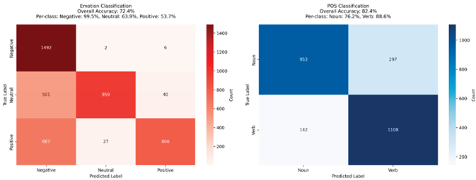
(above) Confusion matrices (CM) for various baseline models (see appendix for model architectures), evaluated on held-out test data related to emotional valence. Left to right: (1) CM for EEGNet inspired model trained on time series data. Reported a ~88% mean accuracy. (2) CM for EEGNet inspired model trained on FFT data (see methods for data collection processes). Reported ~96% mean accuracy and a ~8% mean improvement from the time-series model. (3) CM for EEGNet inspired model trained on FFT data using the mean of 250 samples (see methods). Reported mean accuracy of 49.5% (this model ignored).
Figure 2.
(above) Confusion matrices (CM) for various baseline models (see appendix for model architectures), evaluated on held-out test data related to emotional valence. Left to right: (1) CM for EEGNet inspired model trained on time series data. Reported a ~88% mean accuracy. (2) CM for EEGNet inspired model trained on FFT data (see methods for data collection processes). Reported ~96% mean accuracy and a ~8% mean improvement from the time-series model. (3) CM for EEGNet inspired model trained on FFT data using the mean of 250 samples (see methods). Reported mean accuracy of 49.5% (this model ignored).
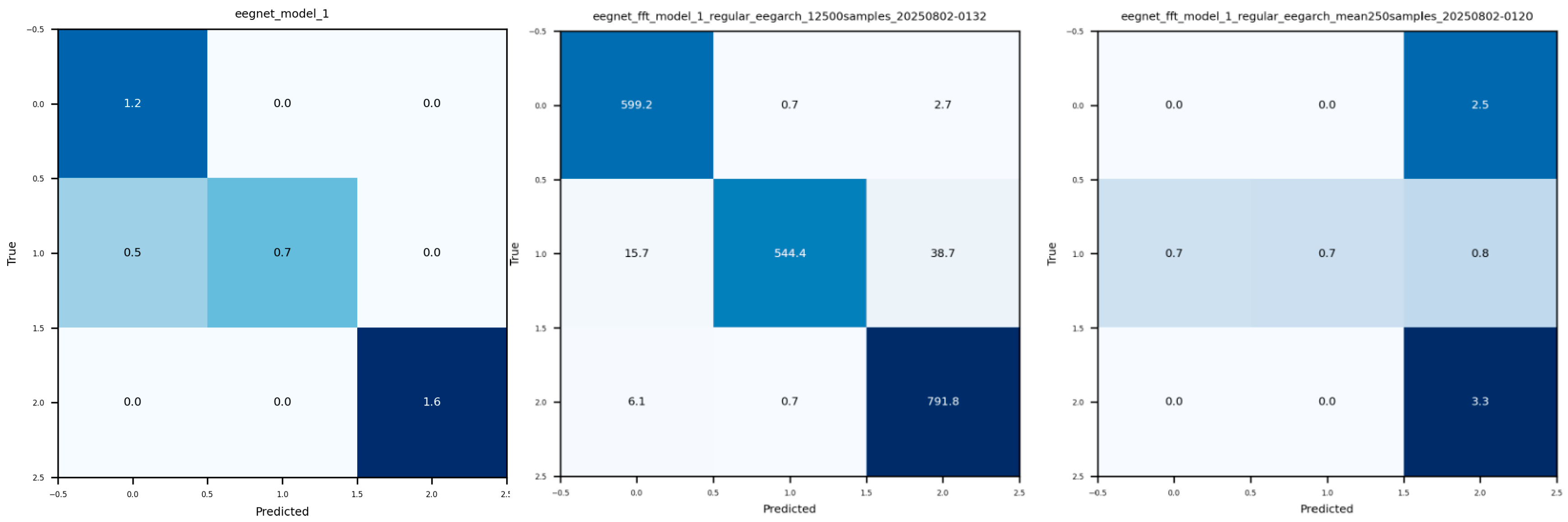
Figure 3.
(left) Graphs of the EEGNet inspired time series model (see Appendix A: Table A4 for architecture) depthwise filter weights. This was the model evaluated in Figure 2 on emotion tasks. This is a spatial filter that learns patterns from each individual channel (see methods). Channel 3 shows distinct, sharp, oscillatory patterns which are all signatures of eye artifacts. This is corroborated by the fact that channels 3 and 4 are frontal electrodes (F7 and F8 respectively).
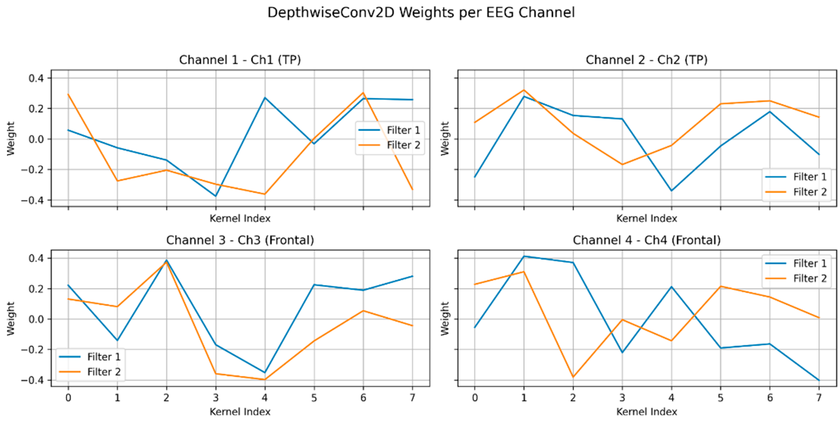
Figure 4.
(above) Graphs of the EEGNet inspired time series model (see Appendix A: Table A4 for architecture) average channel contribution for the model evaluated previously. Using LIME analysis, it’s clear that there is an overreliance on channel 3 (channel 2 on figure) which possesses some artifacts. The model seems to be ignoring channel 1 and 4 (channel 0 and 3 on figure respectively), which likely contains rich EEG information.
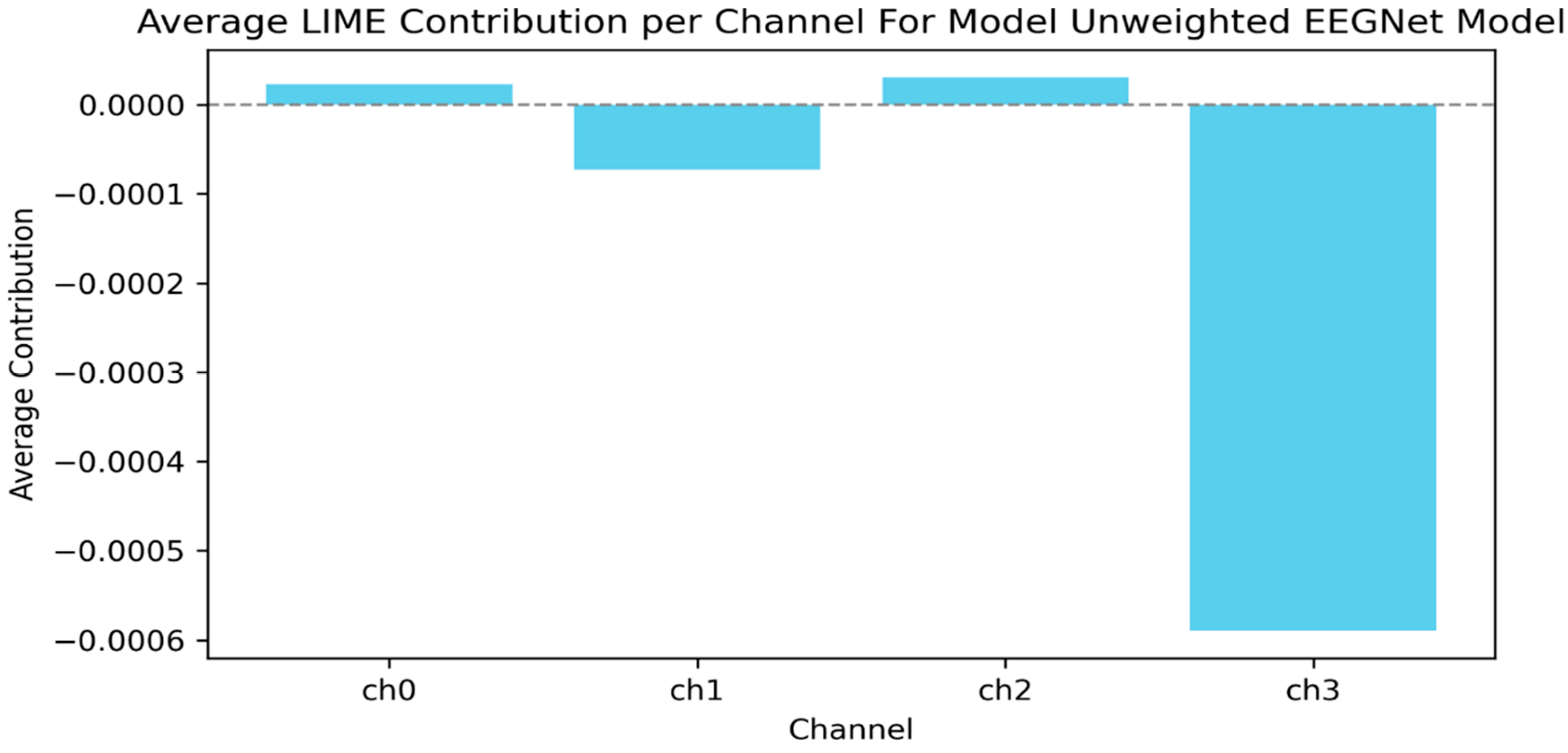
Figure 5.
(left) The CM for the time-series model with weights [1, 1, 0.6, 0.6] is evaluated with a mean accuracy of ~90%. This is a mean increase of ~4 points from the unweighted model. Note, weights were applied during training data and not during testing.
Figure 5.
(left) The CM for the time-series model with weights [1, 1, 0.6, 0.6] is evaluated with a mean accuracy of ~90%. This is a mean increase of ~4 points from the unweighted model. Note, weights were applied during training data and not during testing.
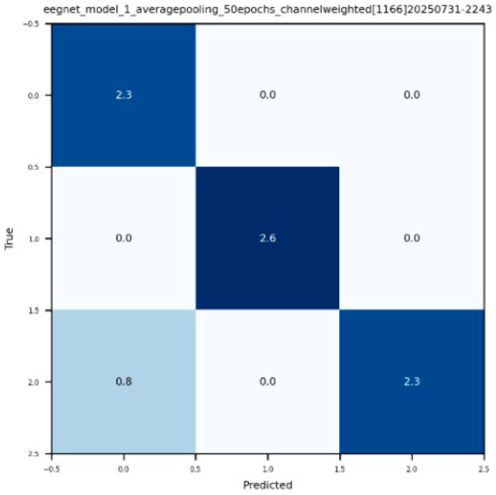
Figure 6.
(bottom-left) The average channel influence on the output is displayed from the LIME analysis for the newly weighted time-series model. An increase in non-artificial channel 2 (chan. 1 on figure) is evident along with a decrease in reliance on artificial channel 3 (channel 2 on figure).
Figure 6.
(bottom-left) The average channel influence on the output is displayed from the LIME analysis for the newly weighted time-series model. An increase in non-artificial channel 2 (chan. 1 on figure) is evident along with a decrease in reliance on artificial channel 3 (channel 2 on figure).
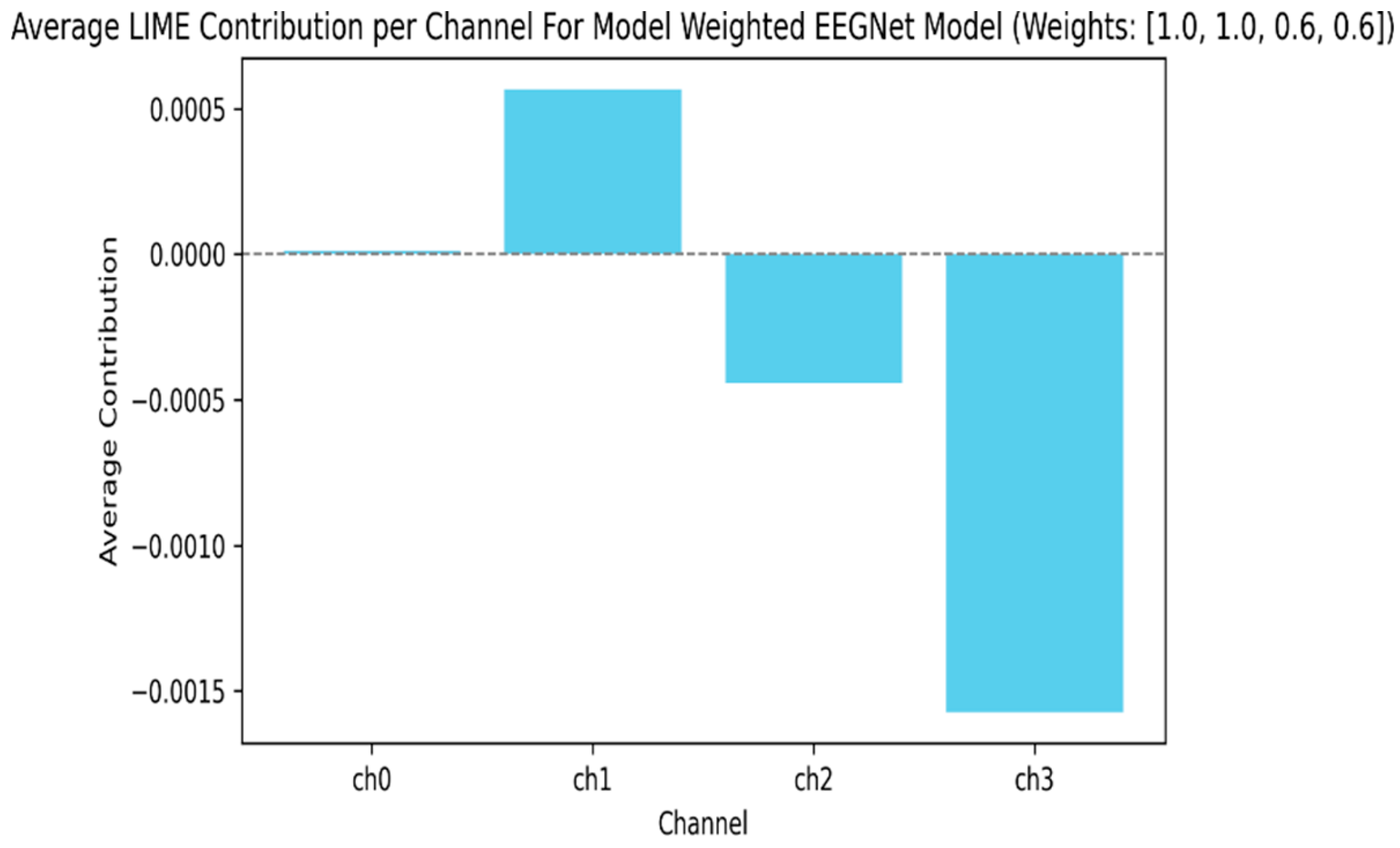
Figure 7.
(left) The LIME analysis for our baseline FFT model is shown. Clearly, it learned to rely more on channels rich in true EEG signals without relying on external weighting.
Figure 7.
(left) The LIME analysis for our baseline FFT model is shown. Clearly, it learned to rely more on channels rich in true EEG signals without relying on external weighting.
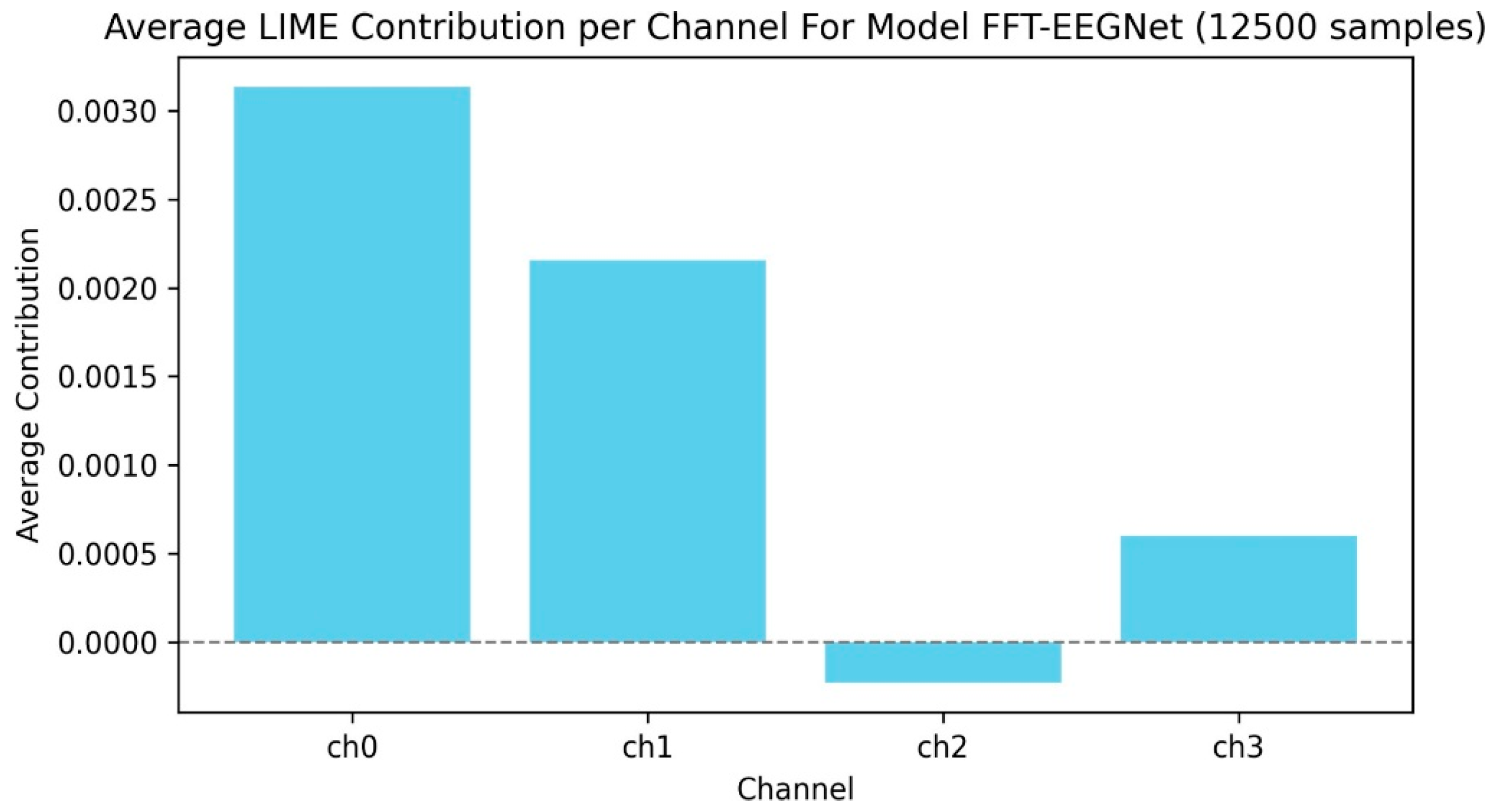
Figure 8.
(above) Multi-head, independent classification mean accuracies are reported in the CM’s above. Compared to the single-task, emotion baseline model the multi-head model performed ~16% worse on emotion tasks. Compared to the single-task, noun/verb (POS) baseline model the multi-head model performed ~9% worse on this specific task.
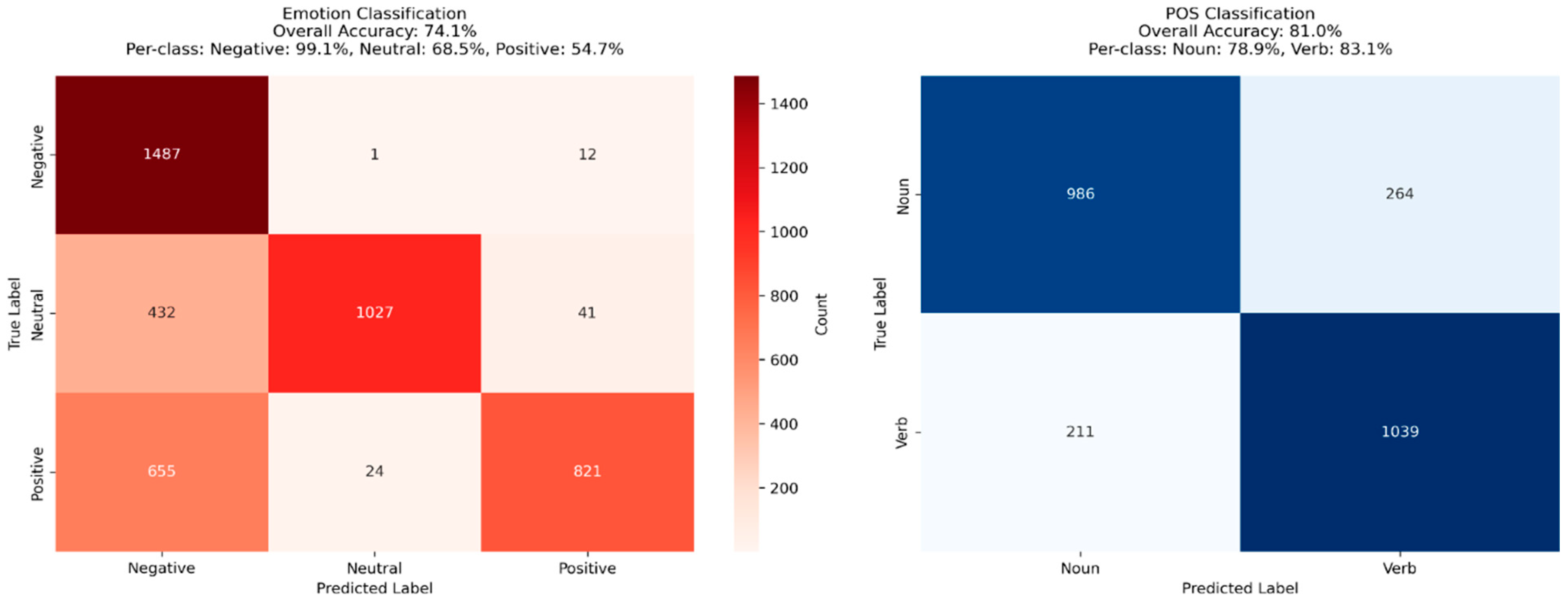
Figure 9.
(below) The baseline multi-head model, after evaluation, was analyzed using LIME analysis and weight visualization. It’s evident that there is a strong reliance on all channels including those likely abundant with artifacts. This could hinder performance, especially on the test data, generalization, or learning true patterns.
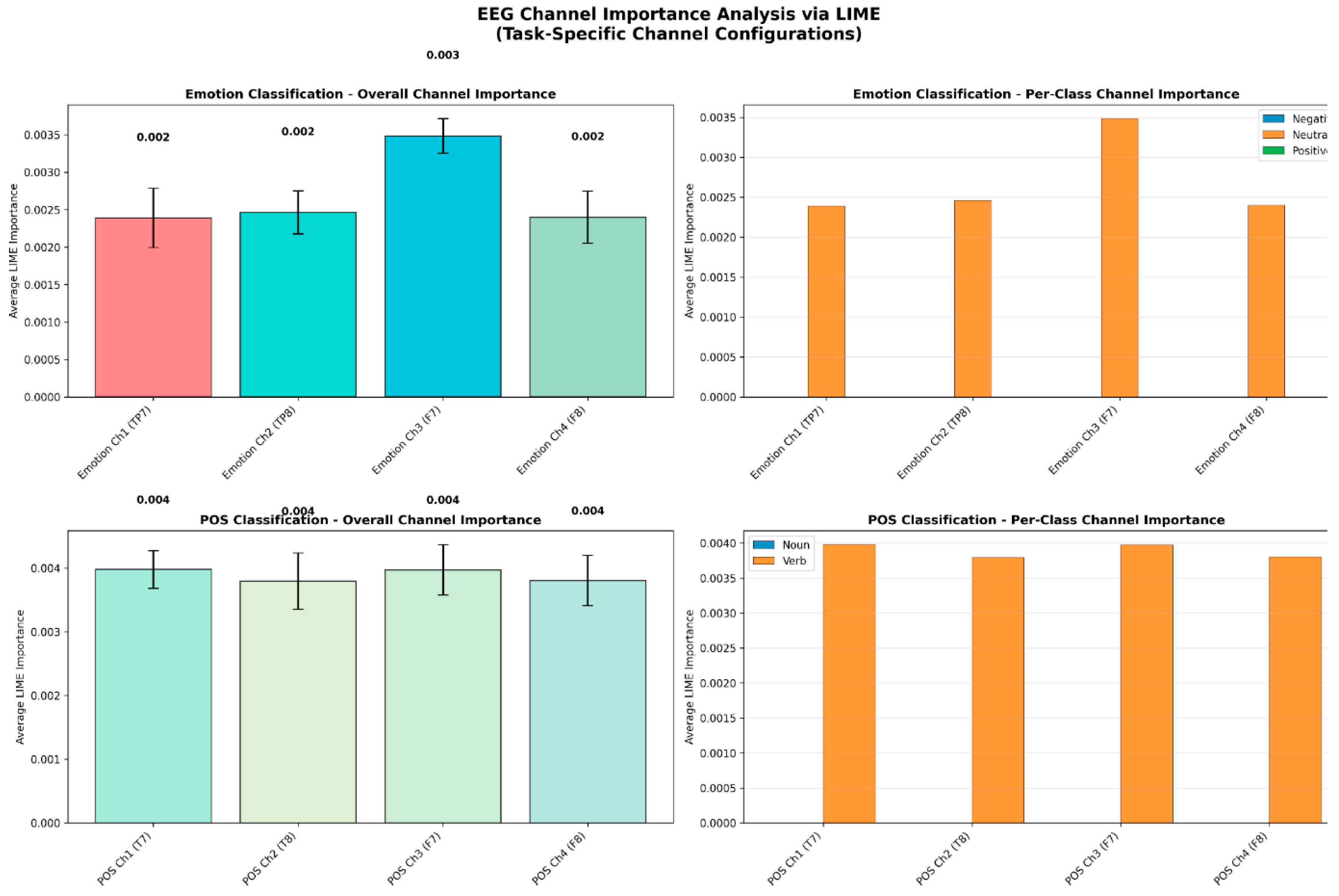
Figure 10.
(above) After weighting by multiplying by [1, 1, 0.75. 0.75] to channels 1, 2 ,3 and 4 respectively,, the multi-head model had a net increase of 0.3% compared to the unweighted multi-head model. For emotion classification (the left), the weighted model performed better by 0.6%. For POS classification, the model accuracy decreased by 0.3%. Overall, the model exhibited very little change relative to its baseline model.
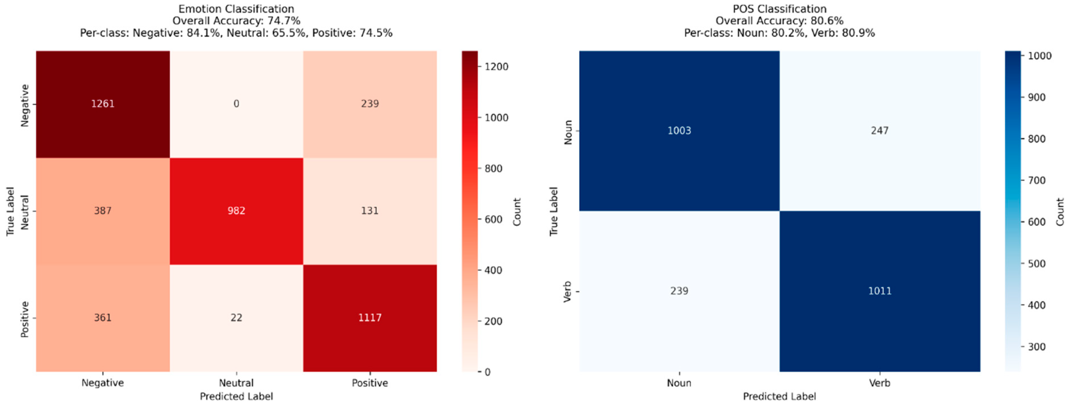
Figure 11.
(below) LIME analysis is shown above for the newly weighted model showing less reliance on channel 3 compared to the baseline multi-head model. However, the weighting still resulted in minuscule improvements in channel reliance and in overall accuracy as seen in Figure 10.
Figure 11.
(below) LIME analysis is shown above for the newly weighted model showing less reliance on channel 3 compared to the baseline multi-head model. However, the weighting still resulted in minuscule improvements in channel reliance and in overall accuracy as seen in Figure 10.
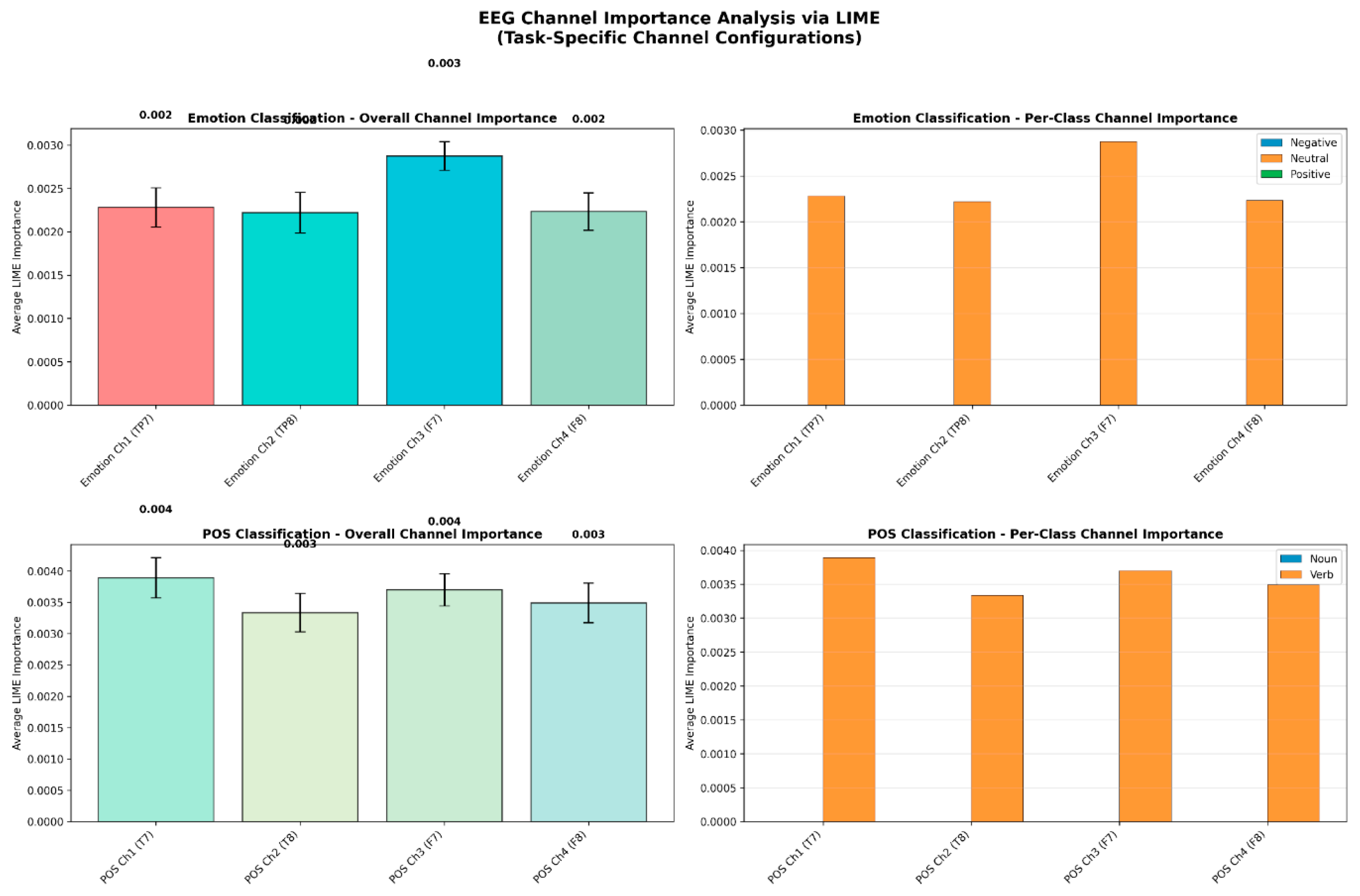
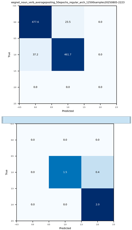
Figure 12.
(below) Shown are the CM’s for both emotion and POS tasks evaluated on the embedding constrained model using held-out test sets (with each set having a random 2500 samples). The clusters showed groups of emotional related words as well as nouns & verbs, and therefore evaluated as such. Both tasks were evaluated independently with POS classification reaching an accuracy of 93.04% and emotion classification reaching an accuracy of 94.16% accuracy.
Disclaimer/Publisher’s Note: The statements, opinions and data contained in all publications are solely those of the individual author(s) and contributor(s) and not of MDPI and/or the editor(s). MDPI and/or the editor(s) disclaim responsibility for any injury to people or property resulting from any ideas, methods, instructions or products referred to in the content. |
© 2025 by the authors. Licensee MDPI, Basel, Switzerland. This article is an open access article distributed under the terms and conditions of the Creative Commons Attribution (CC BY) license (http://creativecommons.org/licenses/by/4.0/).
Copyright: This open access article is published under a Creative Commons CC BY 4.0 license, which permit the free download, distribution, and reuse, provided that the author and preprint are cited in any reuse.


