
Submitted:
23 November 2025
Posted:
24 November 2025
You are already at the latest version
Abstract
The control of wastewater treatment plants (WWTPs), with the ultimate goal of reducing as much as possible the contamination of aquatic ecosystems, constitutes an important multidisciplinary environmental objective. One of the best-known wastewater treatment procedures consists of the use of the so-called Activated Sludge Processes (ASP), which are biological processes that reduce organic contamination thanks to the vital activity of certain bacteria. The control of this type of processes is not easy, precisely due to its biological nature. Consequently, the control of wastewater treatment plants based on ASP processes constitutes an important challenge in the field of Automatic Control, with numerous strategies proposed to date. With the aim of testing and evaluating the different existing strategies, in an objective and orderly manner, the so-called Benchmark Simulation Models (BSM) emerged, which are standard models of wastewater treatment plants based on ASP processes. The main objective of this article is precisely to test the feasibility and evaluate a specific Fuzzy Model Based Predictive Control (FMBPC) strategy, applied to the wastewater treatment plants represented in the BSM1 benchmark (a particular case of the BSM benchmarks). The FMBPC strategy is potentially appropriate for the control of complex, changing or unknown systems and this article demonstrates that this strategy, used in the BSM1 benchmark control configuration (as an alternative to the default control configuration), is viable and performs satisfactorily, to the point that it can even be considered a competitive strategy compared to more traditional control strategies. In the experiments carried out, in a simulation environment, a specific FMBPC control modality has been used, called FMBPC/CLP, which incorporates mechanisms for imposing restrictions on the control action. The base model of the plant to be controlled, necessary for the implementation of the FMBPC strategy, is obtained by prior fuzzy identification of the plant, which is, in our case, the WWTP plant integrated into the BSM1 benchmark itself. The identification procedure developed is based on the information contained in input output data series of the plant in open loop, previously obtained by simulation. Identification is achieved with the help of a software tool that uses mathematical clustering methods, based on the Gustafson Kessel algorithm, through which it is possible to extract Takagi Sugeno type fuzzy models, from numerical input output data of a given plant.
Keywords:
Benchmark Simulation Model no. 1
; wastewater treatment plant
; activated sludge process
; fuzzy model-based predictive control
; closed-loop predictive control
; control of systems with restrictions
; multivariable control
; intelligent control
; fuzzy identification
; Takagi-Sugeno fuzzy models
1. Introduction
The biological purification processes used in Wastewater Treatment Plants (WWTPs), such as Activated Sludge Processes (ASP) [1,2,3], are difficult to control, both due to their own biological characteristics intrinsic, such as strong disturbances that affect the incoming water (flow-rate, pollution, etc.). There are numerous techniques, methods and control algorithms proposed to face such adverse conditions and improve the performance of treatment plants [4,5,6]. However, this branch of science and technology remains open to new contributions. Not only because of the indisputable environmental interest and the need to comply with the legislation that regulates industrial water purification activities, but also because the control of such processes represents an important scientific-technical challenge, almost paradigmatic, in the discipline of automatic control. Within this discipline, some specific areas or lines of research are, at least potentially, quite promising in the search for solutions to improve and refine wastewater treatment processes. Among these, we can cite, among others, the following areas of automatic control: model-based predictive control [7], neural control, fuzzy control, neuro-fuzzy control, intelligent control, and various possible combinations thereof. Likewise, currently, it is worth considering very diverse and imaginative approaches of artificial intelligence (AI) applications or tools applied to the control of wastewater treatment plants. Some examples of contributions in the areas mentioned can be found in [8,9,10,11,12,13,14,15,16,17].
This article analyzes a type of strategy that can be characterized as Fuzzy Model-Based Predictive Control (FMBPC) [18,19,20,21,22,23,24,25,26,27]. This strategy shares common elements with three of the aforementioned subfields of automatic control: model-based predictive control, fuzzy control, and intelligent control. The article addresses the implementation of this strategy, in a simulation environment, applied to the control of wastewater treatment plants based on biological processes of the ASP type. The main objective is to evaluate both the feasibility and the performance of the strategy in such context. The specific control algorithm to be evaluated, of the FMBPC type, was initially proposed in [25]; it was later analyzed from the point of view of stability in [26]; and finally, in [27], it was adapted to be able to consider restrictions on the control action. In the three stages of its development, such a strategy was applied (in simulation) to activated sludge purification processes, considering a simplified WWTP plant. An important motivation of this article is, precisely, to demonstrate that the aforementioned strategy can also be applicable and useful for more complex and realistic plants, with internationally standardized architectures (with evaluation objectives), represented by the so-called Benchmark Simulation Models (BSM) of wastewater treatment plants, and more specifically, through what is known as Benchmark Simulation Model no. 1 (BSM1) [5,6,28]. Some examples of evaluation of control strategies using the BSM1 reference model can be seen in [29,30,31,32,33,34,35,36,37].
In the bibliographic references [25,26,27], the specific FMBPC type control strategy that will be used in this work is described in a broad and detailed manner. Furthermore, the necessary aspects of this strategy are described and developed in section 3 of this article. However, it seems appropriate to include in this introductory section a brief description of its main characteristics. In relation to its initial original formulation, that is, without yet considering restrictions, such characteristics are, in summary, the following: regarding the prediction model, it should be said that this will initially be a fuzzy model expressed in the form of if-then rules, of the Takagi-Sugeno type [38], which must have been obtained through fuzzy identification, from series of numerical input-output data corresponding to the plant to be controlled; on the other hand and subsequently, this model will be adequately reformulated to obtain an equivalent model in the state space, of a discrete, linear and time-varying type (DLTV model), which will be taken as the final prediction model; and in relation to the procedure for deducing the control law, it is relevant to say that typical mechanisms of classical predictive control are not used, such as the minimization of some cost function, but rather concepts and principles of the so-called Predictive Functional Control (PFC) are applied, such as the well-known Equivalence Principle (related in turn to certain concepts, such as: reference trajectory, coincidence horizon and coincidence points) [39,40,41]. Starting from the final prediction model (DLTV model) and conveniently applying the aforementioned equivalence principle, it is possible to deduce the predictive control action, which turns out to be an analytical and explicit mathematical expression, with time-dependent coefficients that must be updated in each iteration (or sampling period) [25]. The fact that the control action is given by an analytical and explicit expression is one of the potentially interesting characteristics of this strategy (in the computational field).
The FMBPC strategy summarized above was subsequently endowed with the capacity to handle restrictions on the increments of the control action (in the vicinity of an equilibrium point), adding to the initial original expression of the control action a complementary additive term, calculated by a certain algorithm that, this one yes, minimizes a certain cost function that takes into account the constraints. We will refer to this control law, more complete, by the acronym FMBPC/CLP [27], where the initials CLP refers, in abbreviated form, to the control strategy originally called Closed-Loop Paradigm, also known as Closed-Loop Predictive Control [42], represented by the initials CLP-MPC. The experiments that form the experimental basis of this article have had the ultimate objective of evaluating the effectiveness of the FMBPC/CLP control law, applied to more complex activated sludge purification processes than those considered in [27].
The application of the FMBPC/CLP strategy to the control of purification processes using activated sludge could be advantageous, compared to other strategies, due to some of its characteristics. Among these, it is worth highlighting the use of fuzzy models based on rules, obtained from input-output numerical data, which can be very useful (and even ideal) to capture the dynamics of complex, variant, or unknown systems, such as the case of ASP biological wastewater purification processes (complex, variants and subject to strong external disturbances). This potential advantage could lead, within a model-based predictive control scheme, to better behavior of the controlled system, both in comparison with classic non-model-based strategies, and in comparison, with other predictive control strategies whose base model is not fuzzy or has not been deduced from input-output data. The analytical and explicit form of the final control law could also provide some computational advantage. And finally, the capacity to incorporate restrictions in the increments of the control action could also mean an improvement in the behavior of the controlled system, compared to strategies that do not have such capacity.
Section 2 of this article describes and explains the reference simulation model for wastewater treatment plants no. 1 (BSM1 benchmark). Section 3 details the necessary and relevant aspects of the FMBPC/CLP hybrid strategy (both its individual components and the combination thereof), as well as its integration into the BSM1 benchmark control system. Section 4 describes the fuzzy identification procedure of the WWTP plant represented by the BSM1 benchmark and presents the results of the identification. Section 5 describes the control experiments conducted with the BSM1 benchmark using the FMBPC/CLP strategy and evaluates, based on the results, both the feasibility of integrating this strategy into the BSM1 benchmark and its performance. Finally, section 6 presents the main conclusions we draw from the research work carried out, as well as possible future work that we consider to be of interest.
2. Benchmark Simulation Models of Wastewater Treatment Plants: The BSM1 Benchmark
The availability of reference simulation models and their standardization, with objectives of evaluation and comparison of different strategies, is an extraordinary tool in any field of scientific-technical research and in particular in the control of wastewater treatment plants, which is especially complex. With this objective, the International Association for Water Quality (IAWQ) and working groups of the European Cooperation in Science and Technology (COST) organization, belonging to the interdisciplinary research networks COST Action 682 and 624, designed and developed, among the years 1998 and 2004, benchmark tools for the simulation-based evaluation of control strategies for activated sludge plants [43,44,45,46]. After 2004, this task was assumed mainly by the IWA (International Water Association) Task Group on Benchmarking of Control Strategies for WWTPs, which promoted new research and development projects in modeling, simulation, and evaluation of wastewater treatment plant control strategies. Among the many fruits of this work, it is worth highlighting the development of reference simulation models for WWTPs, carried out seeking a compromise between simplicity, realism, and standardization, and including the following: the plant layout, a (sufficiently validated) simulation model of the biological and biochemical processes involved, influent loading models, regulated test procedures and, finally, performance evaluation criteria of the control strategies that want to be evaluated. The different models were progressively completed and updated, crystallizing into the following three standard models: Benchmark Simulation Model no. 1 (BSM1), Long-Term Benchmark Simulation Model no. 1 (BSM1_LT) and Benchmark Simulation Model no. 2 (BSM2), whose corresponding descriptions were published in the form of technical reports generated within the IWA association [28,47,48,49,50]. Such descriptions are available on specialized websites, such as: http://iwa-mia.org/benchmarking (of the Modelling & Integrated Assessment working group of the IWA association) and https://wwtmodels.pubpub.org (Wastewater Modeling). The main objective of this last site is to contribute to the centralization and dissemination of scientific publications of different types (technical reports, articles, and literature) related to wastewater modeling, also providing software for the implementation of the BSM benchmarks, stored in a series of Github repositories created specifically for that purpose. Thus, from https://github.com/wwtmodels/Benchmark-Simulation-Models it is possible to download the necessary software for the implementation of the BSM1 and BSM2 benchmarks in the Matlab® and Simulink® environment (for Matlab versions ranging from Matlab R2006 to Matlab R2019b). R2019b).
2.1. Brief Description of the BSM1, BSM1_LT and BSM2 Benchmarks
The BSM1 benchmark addresses the biological treatment of wastewater by means of activated sludge, making use (sequentially) of a compartmentalized biological reactor and a secondary settler (clarifier). A fundamental biological process for purification takes place in the reactor, consisting of the digestion of organic matter by certain types of bacteria, as well as a complementary process of eliminating nitrogen from wastewater (before it is discharged into the river), decomposed into two subprocesses, known as pre denitrification and nitrification. Studies evaluating possible control strategies are carried out in periods of 14 days and different climatic conditions are considered, usually classified into three categories: dry weather, rainy weather, and stormy weather. In the second subsection of this section, below, a detailed analysis of the most important aspects of the BSM1 benchmark is carried out. In addition, the complete description of this reference model can be consulted in: [28,49,50].
The BSM1_LT benchmark is based on the BSM1 model, but with a much longer evaluation period of control strategies (specifically 609 days), which implies the consideration of possible special phenomena, such as toxic events or problems with sensors and actuators, and potential failures derived from them. The complete description of this reference model can be seen in [47].
The BSM2 benchmark has two clearly differentiated parts: one of them aims at the biological treatment of wastewater, and is the same as the BSM1 model, and the other is a supplementary structure for sludge treatment. It is possible to consult the complete description of this model in [48].
2.2. BSM1 Benchmark: Structure, Features, and Default Control Strategy
In Figure 1, the structure of the BSM1 benchmark can be seen schematically, including the fluid streams (water or sludge) that pass through its different structural elements and, in addition, a typical closed loop control configuration, which incorporates separate PI control loops for the variables SNO,2 (concentration of nitrates and nitrites in compartment No. 2 of the reactor) and SO,5 (concentration of dissolved oxygen in water in compartment No. 5 of the reactor), respectively.
The activated sludge biological reactor is divided into five compartments, the first two (from left to right) being perfectly mixed and not aerated (anoxic) and the last three ones being aerated. Following the reactor (in Figure 1, to its right) there is a settler (clarifier), called secondary settler (symbolically represented in two dimensions by a triangle, although its real geometric shape could be a cylinder, with a narrowing at the bottom). The secondary settler is modeled as a 10-layer unit, without biological reactions, assigning to the sixth layer (from bottom to top) the role of feed layer (inlet layer for the water leaving the reactor).
The plant is designed for an average influent flow rate in dry weather of 18,446 m3·d-1 and a biodegradable Chemical Oxygen Demand (COD) in the influent of 300 g·m-3 (on average). The overall volume of the biological reactor is equal to 6,000 m3 and its distribution is as follows: each of the two anoxic compartments has a volume of 1,000 m3 and the volume of each of the three aerated compartments is equal to 1/3 of 4,000 m3. The volume of the decanter is also equal to 6,000 m3 and therefore the total volume of the plant is equal to 12,000 m3. Considering the total volume and the value of the average influent dry-weather flow rate (specified above), the average hydraulic retention time of the plant designed in the BSM1 benchmark will be 14.4 hours.
Each of the streams that complete the process has a pair of variables associated in Figure 1, namely: the variable Q, which represents the flow rate and the vector variable Z, which represents, in a grouped way, the concentrations of the different standard fluid components. These streams must also be included in the description of the BSM1 benchmark. We will first mention the main water current, which follows the following stages: it originates in the influent (Qi), it passes then through the five compartments of the reactor, and subsequently through the settler (Qf) and finally, from the tenth layer of this last structural element, it ends up in the river as effluent (Qe). Secondly, we will deal with the sludge outlet stream from the settler (Qu), which is divided into two streams: on the one hand, a recirculation or recycling stream that transports sludge to the first compartment of the reactor, called the external recycle stream (Qr), and on the other, a stream with sludge that will be discarded, called wastage stream and whose flow rate (Qw) has been set, in the default configuration of the BSM1 benchmark, to 385 m3·d-1, which implies (considering the total amount of biomass present) an age of the system sludge of about 9 days. And finally, we will mention the so-called internal recycle stream (Qint), which is water liquid coming from the fifth compartment of the reactor, and which is also fed back to the first compartment of the reactor. The flow rates of the internal and external recycle streams (Qint y Qr, respectively) are of great importance as possible manipulated variables for control purposes.
In addition to structurally describing the plant represented in the BSM1 benchmark, it is also necessary to specify its functional characteristics, which are basically summarized in the following two: capacity to reduce the degree of organic contamination and capacity to eliminate nitrogen (N), in both cases before the discharge of the treated wastewater into the river. These capabilities are detailed below in more detail.
The capability for reducing organic pollution is, logically, a fundamental objective of wastewater treatment plants (which has been maintained since their origins, before the incorporation of nutrient removal mechanisms) and what is intended is to place the degree of pollution below the maximum levels allowed by environmental legislation. This objective is achieved thanks to various biological processes and biochemical reactions that take place in the activated sludge reactor, carried out by certain types of bacteria that need and use the organic matter present in the water for their own growth, for which it is also necessary the external recycle stream (Qr), which feeds the reactor with sludge (rich in bacteria). And of course, the mechanical sedimentation that takes place in the decanter is also essential, the consequence of which is the separation of the mixture from the reactor into two flows, one of clean water, which goes to the river, and another of sludge, which is divided into two streams, namely: the aforementioned external recycle stream (Qr) and the waste stream (Qw).
In relation to the capability for eliminating nitrogen, it must be highlighted that it is an objective that has great environmental importance, since this chemical element is, together with phosphorus (P), one of the main nutrients of harmful algae and other harmful plants to aquatic ecosystems. Nitrogen removal is achieved through the interrelation of two consecutive biochemical reactions (or stages), namely: denitrification and nitrification. The first reaction, denitrification (also known as predenitrification), takes place in the anoxic tanks (the first two reactors crossed by the influent) and occurs due to the interaction of certain bacteria with nitrates and nitrites (SNO) present in the tanks, under conditions of absence of dissolved oxygen, producing nitrogen in gaseous form (N2) as a result, which is evacuated directly to the atmosphere. The second reaction, nitrification, takes place in the aerobic tanks (located after the two anoxic ones) and occurs due to the interaction, in the presence of dissolved oxygen, of certain type of bacteria with ammonium (ammonium ion and ammonia, represented together using the SNH notation). The consequence of such interaction is the oxidation of ammonium and the production of nitrite and then nitrate (represented together by SNO). The denitrification-nitrification process is completed by recirculating water from the fifth reactor compartment to the first (the internal recycle stream, Qint, previously defined), with the objective of supplying nitrates and nitrites (SNO) to the denitrification stage.
All processes that take place in the treatment plant of the BSM1 benchmark (biological, biochemical, or mechanical) are represented by mathematical models. The mathematical model used to represent the processes that take place in the reactor is the model known as Activated Sludge Model No. 1 (ASM1) [51], which includes 8 different biological processes and 13 state variables (of biological and physicochemical type). This model was initially developed within the International Association on Water Pollution Research and Control (IAWPRC) but was later also adopted and updated by the IAWQ and IWA associations (which can be considered the heirs, successively, of the association IAWPRC). In relation to the processes that develop in the settler, it is not necessary to model biological reactions (because they are not considered, as already indicated at the beginning of this section), but nevertheless, it is necessary to model the mechanical processes that take place in it (as a consequence, ultimately, of gravity), which consist of vertical transfers of sludge between adjacent layers. The mathematical model used by the BSM1 benchmark to describe such mechanical interactions, or what is the same, to represent the dynamics of the solid flux of sludge that takes place (as a consequence of gravity), is based on a certain mathematical function known as double-exponential settling velocity function [52].
The BSM benchmarks provide researchers and specialized users with simulation models of the basic processes that take place in wastewater treatment plants, but they also provide complementary resources, necessary for the comparison of the different control strategies under standardized conditions and criteria, such as: series of numerical data with statistically typical profiles for the variables associated with the inlet stream to the plant (influent), extended simulation models including some default control configuration (typically, PID or PI), and performance evaluation criteria of the strategies used. Thus, with respect to the first type of complementary resources that we have just mentioned, the BSM1 benchmark has several dynamic models for the influent, corresponding to three different climatic conditions, namely: dry weather, rain weather, and storm weather. Each model provides temporal data on the 15 variables associated with the influent (the input flowrate, the input values of the 13 physicochemical and biological variables that describe the state of the purification process, according to the ASM1 model, and the time). These models are available in separate 14-day files, with a separation between samples of 15 minutes (approximately 0,0104 days). In relation to the control strategy, the BSM1 benchmark assumes a certain default configuration (as already advanced at the beginning of this subsection), consisting of the incorporation of a control loop with a Proportional-Integral (PI) type controller, to regulate the variable SNO,2, that is, the concentration of nitrates and nitrites in compartment No. 2 of the reactor, and another control loop, also with a PI controller, to regulate the variable SO,5, that is, the concentration of dissolved oxygen in water in compartment No. 5 of the reactor (see Figure 1). Additionally, the BSM1 benchmark suggests some default reference values for the controlled variables, specifies suitable types of sensors and actuators, and sets operational restrictions for the manipulated variables (minimum and maximum bounds). Finally, in relation to the evaluation criteria, the BSM1 benchmark establishes a set of standardized criteria for performance assessment of both the controllers and the plant. In evaluating the performance of the controllers, the focus is on the measure of their effectiveness with respect to the control objectives at the local level, for each loop, and is carried out by calculating various indices, among others, the Integral of the Absolute Error (IAE) and the Integral of the Squared Error (ISE). Regarding the performance assessment of the plant, the focus is directed towards measuring the degree of achievement of the purification objectives of the treatment plant (as an effect of the control strategy) and assessing the way to achieve it, more or less optimal. The specific way to carry out this evaluation is by measuring the quality of the water leaving the treatment plant (effluent), determining the operating costs (including energy costs), and measuring the variations in the output of the controller. The first of these three evaluation actions, the measurement of the quality of the outgoing water (a transcendental indicator of the treatment plants, logically), is carried out in practice by calculating or determining the following numerical indices: the so-called Effluent Quality Index (EQI), the 95% percentile of the ammonia concentration in the effluent (SNH,e95), the 95% percentile of the total nitrogen concentration in the effluent (Ntot,e95), and the 95% percentile of the concentration of total suspended solids in the effluent (TSSe95). The software packages developed to implement the BSM benchmarks can include scripts (more or less generic) for the calculation of the necessary indices for the performance assessment of both the controllers and the plant. This is the case, for example, of the BSM1 benchmark implementation software, in the Matlab® and Simulink® programming environment, available at the Github web address https://github.com/wwtmodels/Benchmark-Simulation-Models (already cited at the beginning of this section), which includes the aforementioned calculation scripts.
3. Alternative Control Configuration for the BSM1 Benchmark: Use of the FMBPC/CLP Predictive Control Strategy
As already indicated in section 2, the BSM benchmarks, and in particular the BSM1 benchmark, were designed to provide researchers with standard reference simulation models, to test and evaluate their own control strategies of wastewater treatment plants based on activated sludge processes. The fundamental objective of the different strategies has to be, logically, to control the activated sludge process in such a way that the purification of wastewater is as ideal as possible. But to achieve this general objective, different control configurations are possible, which will differ from each other depending on the control strategies or algorithms used, as well as the choice of both the controlled variables, and the manipulated variables. Precisely, the main aim of this work is to test and evaluate the integration within the BSM1 benchmark of a certain control strategy, already mentioned in the introductory section and represented by the acronym FMBPC/CLP [25,26,27]. This strategy combines two different predictive control algorithms, already mentioned also: a main algorithm of FMBPC type and a complementary algorithm of CLP-MPC type. Using the FMBPC algorithm, the basic (or main) part of the control action is calculated and using the CLP-MPC algorithm, a complementary term is calculated, which is added to the main part, with the objective of imposing restrictions on control action increments.
In the first three subsections, we will describe and develop the necessary and most relevant aspects of the different strategies involved: the fuzzy predictive control (FMBPC) strategy, the closed-loop predictive control (CLP/MPC) strategy, and the mixed FMBPC/CLP strategy. Finally, in the last subsection, we will describe the integration of the FMBPC/CLP strategy into the BSM1 benchmark control system, which is the central issue at hand.
3.1. FMBPC Predictive Control Strategy
The control strategy FMBPC was already mentioned and briefly described in the introduction of this article. This strategy is part of the group of fuzzy model-based predictive controllers, within which there are various lines and implementations (some of which can be consulted in the bibliographic references cited in the introduction). On the other hand and from a more global point of view, our strategy is framed (at the same time) within two other broader fields, namely: the field of non-linear model-based predictive control (NLMBPC), on the one hand, and the field of intelligent control (IC), on the other; in this second case, because the prediction model is fuzzy, expressed through rules, which constitutes a modality of qualitative reasoning, one of the characteristics of intelligent systems. Consequently, the FMBPC strategy will inherit some of the main characteristics, advantages, and disadvantages, of both the NLMBPC control and IC control. However, an analysis of these control strategies would exceed the scope of this section and also of this article. Therefore, in this section we will focus only on expanding the description of the FMBPC strategy under evaluation.
The specific FMBPC type strategy that concerns us was initially proposed in [25], where the procedure for deducing such a predictive control law was developed. The starting point is a discrete fuzzy model of the plant, of the Takagi-Sugeno (TS) type, previously identified (by fuzzy identification) from numerical input-output data and expressed by a certain set of if-then rules. Each of the rules represents a local (linear) submodel, while the set of all rules represents the global (nonlinear) model. Equation (1) shows the structure of each of the rules of the TS fuzzy model ( rule, ) for a given output (for multivariable systems, there would be a similar collection of rules for each output), representing (here and in all equations in the article) the instant of time, that is, , with being the sampling period:
where: and are the antecedent and consequent vectors, respectively, of the fuzzy model; is a certain fuzzy set (or value) associated with the component of the antecedent vector (for the rule), which will be characterized by a certain membership function, (); finally, represents the output of the fuzzy model at the sampling instant, expressed by a certain affine function of the consequent vector, (where: ).
The identified TS fuzzy model will not, however, be the final prediction model, as was already advanced in the introduction. The TS model obtained through identification is subsequently converted into a state space model, of the DLTV type, with time-dependent (matrix) coefficients, which must be updated in each iteration or sampling period. And this equivalent model is the one that will finally be used, as the base prediction model, by the predictive control algorithm (with the ultimate objective of generating the control variable in each sampling period). The form of the equivalent DLTV model is shown in equation (2):
where: is the extended state vector at the sampling instant (integrated by the plant outputs, together with certain previously chosen input disturbances); is the extended input vector at , formed by two components, and , both referring to the value of a certain manipulable input variable, at two consecutive instants of time (at the current instant, , and in the previous one, ); is the output vector at (formed by the plant outputs); and, finally, , , , and are the different matrices of the model in the state space (dependent on and therefore on time). The detailed composition of all the vectors and matrices that appear in equation (2) can be consulted in [25].
Making use of the prediction model represented by equation (2) and conveniently applying the so-called equivalence principle and other concepts, such as reference trajectory and coincidence horizon (related to functional predictive control), in [25] was deduced a predictive control law of FMBPC-type, analytical and explicit. The corresponding mathematical expression is shown in equation (3):
where: is the appropriate control variable at the instant, calculated by the control algorithm; is the so-called coincidence horizon (); , , and are the output variables (vector type, in the case of multiple output) corresponding to, respectively, the reference trajectory (or trajectories) at the instant , the output measured at time , and the output predicted by the prediction model for time ; is the extended state vector at time ; , , and are some of the matrices of the model in the state space (also dependent on ); is the identity matrix (of the order that correspond); is an operational numerical matrix equal to ; and, finally, is a certain matrix expression, whose composition we do not specify for simplicity (see [25]), which involves, among others, the matrices , , and of the model in the state space.
The FMBPC control law shown in equation (3) depends (at the instant) on the following: on the predetermined reference trajectories for the evolution of the outputs; of the predictions for the output given by the prediction model; of the measurement at the instant of the output itself; of the model matrices in the state space (time-dependents); and, finally, of the coincidence horizon (an integer greater than or equal to ). This last dependence makes an important numerical parameter of the FMBPC strategy at hand, something that must be taken into account when carrying out predictive control experiments based on this control law (whether in simulation or in real time).
In [26] the deduction of the DLTV model of the plant shown in equation (2) was reconsidered. From certain formal mathematical changes, another equivalent DLTV model was obtained, which we show in equation (4):
where: and represent the new state vector (integrated only by the plant outputs) at time instants and , respectively; is the extended input vector (the same as that of the DLTV model represented in equation (2)); is the vector constituted by certain input disturbances previously chosen; is the output vector (formed by the plant outputs); and, finally, , , , and are the different matrices of the new model in the state space (dependent on and therefore on time). The detailed composition of all the vectors and matrices that appear in equation (4) can be consulted in [26].
Likewise, assuming that there are equilibrium points of the open-loop plant (at least one) and taking one of them as a reference, in [26] a new model was deduced, at a local level, valid only for states sufficiently close to the chosen stationary state. In this deduction, the global DLTV model shown in equation (4) was used and was taken into account the requirement that any state of a discrete system must meet to be considered stationary (maintenance at the instant of its value at time , for any ). The deduced model has the following characteristics: it is a model expressed in the state space, local (as already mentioned), incremental, discrete, linear, and time-invariant (DLTI model). This model is shown in equation (5), where its agreement with the standard form of the discrete linear models in the state space can be seen (which implies analytical and computational advantages):
where: , and are certain matrices of the system (inherited from the steady state, under certain assumptions) that depend on the sampling instant; is the state variable (incremental) at time and is the same variable, but at ; is the extended (incremental) input variable at ; and finally, is the output (incremental) variable at . The values of all the incremental variables mentioned refer to the increments with respect to the corresponding values at the equilibrium point. More details on the deduction of this model can be found in [26].
The local model expressed mathematically in equation (5) is equivalent, in the vicinity of some previously chosen stationary state, to the global model from which it is derived, previously expressed in equation (4), and this, for its part, is equivalent to the model shown in equation (2) (the original model), from which the predictive control law of the FMBPC type that we are describing in this section and which was shown in equation (3) (in its original formulation) was deduced. With respect to this law, in [26] it was demonstrated, using the mathematical relationship between the different models involved, that such FMBPC control law could be expressed, for the local incremental model shown in equation (5), by the following mathematical expression:
where: is an expression, which depends on the sampling instant, where the different factors that make it up are matrices or matrix expressions related to the mathematical models involved and whose specification we do not include (for simplicity reasons); for more detail, see [26]. The form of the control law shown in equation (6) is analogous to that of the well-known state feedback law, given generically by the following expression (equation (7)(7)):
The form of equation (6) (the same as that of equation (7)(7)) reinforces the consideration made above (on the occasion of the deduction of the model shown in equation (5)), in the sense that the deduced mathematical expressions for the local model provide analytical and computational advantages. This statement is based, on the one hand, on the intrinsic simplicity of such expressions and, on the other hand, on the fact that both the model shown in equation (5), and the control law shown in equation (6), or in the equation (7), are part of the theory of linear control systems, widely known and developed and equipped with analytical methods and computational procedures that are simpler than those of the theory of nonlinear control systems. In other words, since we are assimilating our non-linear control system, based on a FMBPC type law, to a linear control system (at a local level, of course), then we will be able (at such a local level) to use and advantageously take advantage of the analytical methods and computational procedures (in predictive control) developed and tested for these systems, which are simpler and better known than the corresponding methods and procedures of the theory of nonlinear control systems.
3.2. CLP-MPC Predictive Control Strategy
The CLP-MPC algorithm, conceptually known as Closed-Loop Predictive Control, is a particular case of the strategy called Dual Mode Predictive Control, represented by the acronym DM-MPC [42]. We will briefly describe both the framework strategy, DM-MPC, and the particular case, CLP-MPC. But previously we will detail (below) the minimum necessary mathematical basis.
The mathematical formalization of the DM-MPC and CLP-MPC strategies has as its starting point the adoption of a certain standard representation of the open loop plant, as well as the choice of a certain typical control law. The open loop plant is represented by a linear model in the state space, of a standard nature, whose form is shown below, in equation (8):
which can be reformulated with a more abbreviated notation (for formal simplification purposes), as shown below, in equation (9):
where: is a vector variable that represents the state of the system at the instant of time (generic); , the manipulable input or inputs, in ; , the output or outputs of the plant, in ; and, finally, , and represent the matrices of the system in the state space. If the system is multivariable, and can be vector variables (both or only one of them). In relation to the choice of some control law for this system, it should be said that a widely used solution is the choice of the so-called state feedback law, whose form is the following:
where: is a certain dimensionally appropriate matrix factor (that is not must confused with the temporal variable ), to be chosen or determined by some criterion. On the other hand, once this law is assumed, it is common to also carry out the formal definition that we show below, in equation (11):
which is appropriate to simplify the mathematical developments associated with predictive control. If expression (10) is substituted in the model defined in equation (9), obtaining as a consequence the mathematical expression of the closed-loop model, the suitability of such definition will be understood.
DM-MPC predictive control, also called Open Loop Paradigm (OLP), consists of considering the prediction horizon divided into two different consecutive sections, called mode-1 and mode-2, whose difference lies in the type of control action planned for each of them. In the first section (mode-1), which covers the first steps (where is a previously set integer), the control actions are not predetermined and will be obtained through optimization, minimizing some cost function. These actions constitute the degrees of freedom of control configuration (d.o.f., abbreviated) and they depend on the instant of time . At each instant of time the next control actions (including the control action) that minimize the cost function must be calculated (jointly). For their joint formal representation, we will use the following mathematical notation: , where the compound subscript indicates that this is a calculation made at (of the optimal control actions), for the following instants (or steps), including instant itself. In the second section (mode-2), which begins at step and extends to the last step of the prediction horizon, the step ( being another integer, previously set as well, satisfying ), the control actions will be calculated by applying some closed-loop control law, for example of the type, with being the state (see equation (10)). Using the same type of notation as in the first section, we can represent the control actions of the second section in the following way: . The ordered union of the control actions of both sections constitutes the global sequence of control actions that will be considered in the predictions, from the first step of the prediction horizon to the last. Such global sequence must be optimized jointly, thus determining the optimal values of the degrees of freedom of the control problem (the first control actions). And once that is done, the first value of the global optimal sequence of actions obtained will be the one that will be taken for the effective control action at the sampling instant, .
In the so-called closed-loop predictive control, CLP-MPC, the control actions planned for the second section of the predictions (mode-2) are defined in the same way as those for the second section of the dual-mode predictive control, DM-MPC, that is, its mathematical expression will be the one corresponding to some closed-loop control law, for example of the type. However, the control actions predicted by the CLP-MPC algorithm for the first section of the predictions (mode-1) are different from those of the general DM-MPC strategy for the same section, being expressed, at each step, as the sum of two mathematical terms, namely: a first term corresponding to some previously fixed closed-loop control law (generally the same as in mode-2, for example, ) and a second term, which we will represent with the notation , known as perturbation of control action and which must be determined by means of an optimization procedure, with constraints in the control action or, as in the case at hand, in its increments. These complementary variables constitute (considered together) the degrees of freedom of the optimization problem. Taking into account the description just made, relative to the control actions planned in , and also taking into account the form of the base model of the plant, specified in equation (9), as well as the definition contained in equation (11), the prediction model of each of the two modes or sections of the CLP-MPC predictive control will be expressed (in relation to the state and the control actions) as detailed below (equations (12) and (13)):
Using now equations (12) and (13) we can now easily deduce the matrix expression corresponding to the sequence of control actions planned, at the sampling instant, for the entire prediction horizon. The expression obtained, which we will represent using the notation , is the following:
where the degrees of freedom (d.o.f.), expressed in matrix form and using the notation , are the following:
The description of the CLP-MPC predictive control algorithm is based on the equations (12), (13), (14) and (15) specified above (which constitute the minimum necessary mathematical basis), but its complete description would require a more extensive development that would excessively overload the article and therefore will not be included here (see [27,42]). However, it seems appropriate to briefly summarize this procedure. The following would be necessary: deduce the matrix expressions (corresponding to the entire prediction horizon) of the state, on the one hand, and of the control action, on the other, and formalize them as a function (a different function for each of the two variables) of the degrees of freedom, that is, as a function dependent on the matrix (which will be expressed below with the simpler notation ); define a certain cost function, which we will denote as , according to some previously established criterion, and express it also as a function dependent on ; specify the restrictions (in our case, restrictions on the increments of the control action) and pose the appropriate optimization problem, generally consisting of finding the minimum of the cost function , while satisfying the imposed constraints. Such an optimization problem can be expressed in an abbreviated form as shown below, by equation (16), where the degrees of freedom are the set of elements of and the acronyms mean subject to:
The solution to the problem expressed in equation (16) will provide as a result an optimal sequence , which we will represent with the notation (where the letter , in the subscript, refers to the constraints). The first element of the optimal sequence obtained, which we will denote with , will be the complementary term that must be added to the expression of the base control law corresponding to the first step of the prediction horizon (associated with the instant), obtaining as a result the complete optimal control action for that first step, which will be the one that the predictive control algorithm will ultimately adopt as the effective control action at the sampling instant. Such control action, which we will denote with , will be expressed, in accordance with what has been explained, by the following equality:
3.3. FMBPC/CLP Mixed Predictive Control Strategy: Implementation
As previously indicated, with the acronyms FMBPC/CLP we are referring to a specific predictive control strategy with constraints that combines the FMBPC and CLP-MPC algorithms, hence the name mixed predictive control algorithm. This strategy was proposed and developed in [27], applied (in a simulation framework) to the control of a wastewater treatment process using activated sludge, represented by a simplified model. The objective of this subsection is to include in this article a summary description of the implementation procedure (in simulation) of the aforementioned strategy. In essence, the implementation procedure of the FMBPC/CLP strategy consists of successively and appropriately applying the predictive control algorithms FMBPC and CLP-MPC. We will describe this implementation procedure below, which will consist of a time sequence that must be carried out cyclically, in each sampling period.
Initially, will be applied a FMBPC type algorithm , which uses as a prediction model a global model of the plant, in the state space and of the DLTV type, resulting from the conversion of another previously determined global model, of the fuzzy type, identified from numerical input-output data (which in our case will also have been obtained by simulation). As a result of the application of the initial FMBPC algorithm, the value of a certain global predictive control action will be obtained, whose mathematical expression was shown previously in this article, in equation (3), identified with the notation . We will rename such control action in this subsection with the following notation: .
Next, and in order to impose restrictions on the control action, will be used (after a series of necessary prior calculations) a second predictive control algorithm, but now of the CLP-MPC type. In order to apply this algorithm, it will be necessary to have, previously, a standard linear model of the plant, of the DLTI type, which will be used as a prediction model, and a standard base control law (both mathematical resources will be used in the calculation of the predictions). The first is possible if we assume that, at the current time instant (the one corresponding to the sampling), the state of the system is in the vicinity of some stationary state, because then, as demonstrated in [26], the plant could be represented (locally) by a standard linear incremental model in the state space, of the DLTI type (equation (5)). This will be the model that will be taken as the prediction model in the CLP-MPC predictive control structure. As for the base control law, in [26] it was shown that, with the plant represented by the equivalent linear model (local scope and DLTI type) represented in equation (5), the FMBPC control law shown in equation (3) (3) is equivalent (locally) to a standard state feedback law of type , as shown in equation (6). This law will be the one taken as the base control law in the CLP-MPC predictive control structure.
The two structural elements required by the CLP-MPC algorithm (both the incremental DLTI prediction model and the base control law) will be deduced after the calculations associated with the FMBPC algorithm have been performed and will be transmitted to the CLP-MPC structure, before this algorithm is executed (these are the necessary prior calculations mentioned in the previous paragraph). This must be done in each sampling period since both elements depend on the sampling instant. The DLTI incremental model is characterized by the matrices , and (equation (5)) and the base control law, by the factor (equation (6)). Therefore, in each sampling period, these four parameters must be updated and transmitted to the CLP-MPC structure. With this numerical information it will be possible to apply, at each sampling instant and for the appropriate local area, the CLP-MPC predictive control algorithm, obtaining as a result the value of the (incremental) control action that will satisfy the restrictions imposed in the optimization procedure (optimal control action). The mathematical expression corresponding to such control action was already shown in equation (17), at the end of the previous subsection, dedicated to the description of the CLP-MPC algorithm independently. But in the present subsection the successive and combined application of two algorithms is addressed, first the FMBPC algorithm and then the CLP-MPC algorithm, and therefore it seems convenient to modify the notation to differentiate both cases. The expression corresponding to the optimal control action is shown below (equation (18)), with the new notation:
where: is the optimal incremental control action; is the state variable corresponding to the local incremental model, of DLTI type, described in equation (5) (having represented the state by the simpler notation ); is the base control law, obtained from the FMBPC algorithm, in its equivalent local and incremental form, for states sufficiently close to the reference steady state (equations (6) and (7)); is the optimal perturbation of the base control action, calculated by the CLP-MPC algorithm and whose role is to ensure that the control action satisfies the imposed restrictions (this term will be the first element of the optimal perturbation vector or matrix, represented in the previous subsection with the notation , which will be determined by solving the corresponding optimization problem); finally, represents the sampling instant.
Finally, once the incremental optimal control action, , has been determined, it will be necessary to determine the absolute optimal control action corresponding to the FMBPC/CLP strategy, which we will denote as . To do this, we will have to add to the value of the global control action FMBPC corresponding to the steady state taken as a reference, ; we will refer to this control action with the notation . That is, the mathematical expression that specifies how is calculated is the following:
and replacing (equation (18)) and grouping appropriately, we will have:
where, to arrive at the final expression, it has been taken into account that is the sum of the following two terms: the first term, , is the equivalent form of the incremental FMBPC control action corresponding to (local incremental state); and the second term, , represents the FMBPC (global) action corresponding to the considered steady state, . From the meaning of both terms, it can be deduced that their sum is equivalent to the predictive FMBPC (global) control action corresponding to the absolute (non-incremental) state , which we had already referred to in the second paragraph of this subsection, with the notation . Consequently, the sum of the two terms can be replaced by , as has been done in the last line of equation (20), thus obtaining the final expression corresponding to the mixed predictive control action FMBPC/CLP.
As can be deduced from equation (20), the procedure for determining the mixed predictive control action at the sampling instant, , will consist of carrying out the following sequence: first, the predictive control action FMBPC (global), , must be calculated; then, using the CLP-MPC algorithm, the optimal incremental perturbation must be calculated (the objective of which is to ensure compliance with the restrictions imposed on the control action); and finally, both values must be added. In the simulation experiments carried out for the occasion of this article, the expression used to calculate the mixed predictive control action (at each sampling period) is precisely the one given by equation (20).
The sequence of calculations leading to the implementation of the FMBPC/CLP strategy, described in this subsection, can be seen schematically in Figure 2 of this article, where the variable represents the set of the controlled variables, grouped vectorially, and the variables and refer to the considered plant input disturbances. The implementation procedure of this strategy can also be seen in algorithmic form in [27].
Regarding the FMBPC/CLP strategy described, it seems appropriate to also include in this subsection a brief assessment (without going into detail, as this would exceed both the scope and the main objectives of this article) of two important aspects from an analytical point of view: the stability analysis of the strategy and its linear or nonlinear nature (see [26,27]). Regarding the former, and in relation to the stability of the base FMBPC strategy, an extensive study demonstrating its local stability is presented in [26]. And regarding the stability of the complementary CLP-MPC strategy, in [42] states that the CLP-MPC algorithm will lead to the stability of the controlled system in closed-loop if the base control law is stabilizing in closed-loop (as is the case with the standard state feedback law of the type , which is the one used). Regarding the second point, the following two considerations must be made: first, that the basic FMBPC strategy is clearly nonlinear, and second, that although a linear (incremental) model is used to determine the complementary control action CLP-MPC in each sampling period, this model depends on the sampling instant, that is, it is different for each period, and must be updated in each iteration.Therefore, in conclusion, we can consider the described strategy as, globally, nonlinear.
3.4. Integration of the FMBPC/CLP Strategy in the Control System of the BSM1 Benchmark
Keeping the same basic control objectives as those of the default control configuration of the BSM1 benchmark (Figure 1), that is, the reduction of organic pollution of wastewater, as well as the simultaneous removal of nitrogen, an alternative control configuration is proposed, with some differences with respect to the classical configuration. The main difference has to do with the use of a controller different from the traditional PID (in one of the control loops), specifically a FMBPC/CLP type controller, which is essentially, as we already know, a combination of two different predictive controllers, namely: a FMBPC controller, that is, a predictive controller based on a certain (internal) fuzzy model of the plant (which must have been previously defined and obtained, through fuzzy identification, from numerical input-output data of said plant), and a CLP-MPC type controller, that is, a closed-loop predictive controller. In relation to the control loops and the controlled variables, the alternative configuration keeps unchanged the control loop for the dissolved oxygen in the fifth tank of the reactor, based on a PI controller, but, nevertheless, replaces the PI control loop for nitrate (in the second anoxic tank) by a multivariable control loop of FMBPC/CLP type, whose objective is to control, not only the nitrate in the second tank, but also, simultaneously, the ammonia in the fifth tank. As for the manipulated variables, the alternative configuration uses the same two variables as the default configuration, as follows: the oxygen transfer coefficient, to control (using a PI controller) the dissolved oxygen concentration in the fifth compartment of the reactor, and the internal recycle flow rate, to simultaneously control (using a FMBPC/CLP controller) the concentrations of both nitrate in the second tank and ammonia in the fifth. The alternative control configuration proposed for the BSM1 benchmark is shown in full in Figure 3.
The structure of the alternative control configuration proposed for the BSM1 benchmark implies a certain increase in complexity with respect to the default control configuration. Consequently, it seems appropriate to clarify and expand the information contained in Figure 3. To do so, we will include the following in this subsection: firstly, a table (Table 1) where the different variables involved in each of the two control loops of the alternative control configuration are detailed in an orderly and structured manner, as well as the role of each of these variables; and secondly, a sufficiently detailed description of each of the two control loops.
where:
Oxygen Control Loop
SO,5 : dissolved oxygen concentration in the fifth reactor unit
SO,5 (measure) : measured value of SO,5
SO,5,ref : reference value (set point) of SO,5
PI output : control variable calculated by the PI algorithm
KLa5 : oxygen transfer coefficient (fifth reactor unit)
Nitrate and Ammonia Control Loop
SNO,2 : nitrates and nitrites concentration in the second reactor unit
SNO,2 (measure) : measured value of SNO,2
SNO,2 (S.P./Ref.Traj.) : reference value (set point), and reference trajectory, of SNO,2
SNH,5 : ammonia concentration in the fifth reactor unit
SNH,5 (measure) : measured value of SNH,5
SNH,5 (S.P./Ref.Traj.) : reference value (set point), and reference trajectory, of SNH,5
d1, d2 : plant input disturbances; in this work, d1 ≡ Qi (influent flow rate) y d2 ≡ SS(i) (concentration of easily biodegradable substrate in the influent)
: control variable calculated by the FMBPC/CLP algorithm
Qint : internal recycle flow rate (originating from the fifth reactor unit)47252525
Regarding the control loop for the dissolved oxygen concentration in the fifth tank of the reactor (variable SO,5), It should be noted (as already indicated at the beginning of this subsection) that this loop has remained unchanged with respect to the original configuration of the BSM1 benchmark. The control action is determined by a PI controller which has two inputs and one output. The inputs are the following: the measured value of the dissolved oxygen concentration in the fifth reactor unit (SO,5 (measure)) and the reference value (set point) of that same variable (SO,5,ref). As for the output, it is about the control variable calculated using the PI algorithm, which will influence, through a valve placed after the controller, in the oxygen transfer coefficient of the fifth reactor unit (KLa5), which is the manipulated variable of this loop.
And as for the second control loop, it is necessary to clarify, first of all, that it is a multivariable loop, whose objective is to control the nitrate concentration in the second tank (variable SNO,2) and, simultaneously, that of ammonia in the fifth (variable SNH,5). And, secondly, it should also be noted that this loop is based on a FMBPC/CLP type controller, with six inputs and one output. The six inputs are as follows: on the one hand, the measurements of the two controlled variables (SNO,2 (measure) and SNH,5 (measure), both given in g∙m-3); on the other hand, the reference values (set point) of these two same variables, together with their corresponding reference trajectories (SNO,2 (S.P./Ref.Traj.), for nitrate, and SNH,5 (S.P./Ref.Traj.), for ammonia); and, finally, two variables whose role is that of plant input disturbances, selected from the variables that define the influent dynamics (d1 y d2). In the implementation, through simulation (Simulink® environment), of the alternative control configuration for the BSM1 benchmark, these two variables are obtained by means of a disturbances selector block that has as inputs the measurements of all the variables associated with the influent and as outputs, only the measurements of the two selected variables (Figure 3). In the present work, the disturbances chosen were the following two: the influent flow rate (d1 ≡ Qi, given in m3∙d-1) and the concentration of readily biodegradable substrate in the influent (d2 ≡ SS(i), given indirectly in g COD∙m-3, where the acronyms COD stands for Chemical Oxygen Demand). Finally, regarding the only output of this second loop, it must be said that it is the control variable calculated by the FMBPC/CLP algorithm (), which is sent to a flow control valve, whose mission is to regulate the internal recirculation flow (Qint, given in m3∙d-1), which is the manipulated variable corresponding to this loop.
To conclude this subsection, we will refer to the sensors and actuators used in the alternative control configuration. Regarding the sensors, for the variables SO,5 and SNO,2 the same types of sensors were used as those considered in the default control configuration (class A and class BO sensors, respectively). For variable SNH,5, however, we decided to consider an ideal sensor (no noise, no delay) in this first attempt at implementing our strategy in the BSM1 benchmark. Regarding the actuators of the two control loops described above (valves, in both cases), it should be noted that, just as in the default configuration, in the alternative configuration were also considered ideal actuators. In practice, in a simulation context (in our case, Simulink®), this is achieved by choosing actuators whose transfer function is such that variations in the manipulated variable are almost a direct translation of variations in the control variable.
4. Fuzzy Identification of WWTP Represented by the BSM1 Benchmark
As already mentioned, the predictive control strategy considered in this article (FMBPC/CLP) uses a fuzzy model of the plant, formalized in state space, as its base prediction model. The fuzzy model is obtained by fuzzy identification, using input-output numerical data series from the plant to be identified, in open-loop configuration. These numerical data, which implicitly contain objective information on the plant dynamics, are obtained, in our case, by performing simulation experiments consisting of applying appropriate input signals to the plant and then measuring the appropriate outputs, depending on the model to be identified [25].
The simulations for obtaining the input-output data of the plant to be identified (the plant represented by the BSM1 benchmark) were carried out in the Matlab® & Simulink® environment and the fuzzy identification was carried out with the help of the software tool called Fuzzy Modeling and Identification Toolbox (FMID) [53], which was developed by its authors as a support for the development and implementation of certain theories and techniques of fuzzy modelling and identification [54]. Within the framework of our particular software development, the FMID tool was partially adapted to cover certain calculation objectives (necessary for our line of research). Through the use of this toolbox, which uses clustering mathematical methods based on the algorithm of Gustafson-Kessel [55], it is possible to extract fuzzy models of Takagi-Sugeno type [38] from input-output numerical data of a given plant. The toolbox supports the selection of various parameters, including those that define the dynamic structure of the (recursive) model to be inferred. The choice of such parameters should be made at the initial stage of the identification process, as a hypothesis, before expressly using the available input-output numerical data. This prior parameterization may be a consequence of some type of prior knowledge or simply obey experimental approaches.
We will describe below (in the successive subsections of this section) the different phases of the identification process carried out: first, the selection of the base model representative of the plant, with regard to its input-output structure; then, the procedure for obtaining the necessary input-output numerical data; and, finally, the identification procedure itself.
4.1. Representative Base Model of the Plant: Input-Output Structure
The plant we want to identify is the wastewater treatment plant represented by the BSM1 benchmark. However, it’s important to clarify that both the control loop for the dissolved oxygen concentration in the fifth tank (equipped with a PI controller), and the actuator needed to regulate the internal recirculation flow rate (a flow control valve), have been considered included in the BSM1 plant.
Once the plant has been defined, it is necessary to define the input-output structure of the model that we want to represent the plant, something that is crucial in the framework of any model-based predictive control strategy. The input-output structure chosen for the base model is shown in Figure 4, where it can be seen that it is a model with three inputs (two disturbances and one control variable) and two outputs (the two variables we want to control).
The input variables with a role of disturbances in the model in Figure 4, generically named d1 and d2, are, respectively, Qi (influent flow rate at the plant inlet) and SS(i) (concentration of easily biodegradable substrate in the influent). Both are part of a broader set of physicochemical and biological variables that characterize the influent [28,49] and whose values, called influent data, will influence the evolution of the biological purification process. Equation (21) shows a list with the 14 variables mentioned (expressed with the standard notation), where the two variables chosen as input disturbances of our model, SS(i) (in the list, SS) and Qi (in the list, Q0), appear in the 2nd and 14th positions, respectively (going through the list from left to right). Likewise, Table 2 specifies the description of each of these 14 variables (13 of which, the first 13, coincide with the state variables of the model that describes the purification process that takes place in the biological reactor, that is, the ASM1 model [51]).
All the variables detailed in Table 2 share the role of plant input disturbances, but only two of them were taken into account in the base model chosen for the predictions. If all of them were taken into account, the complexity of all the procedures (numerical, computational, and software) involved in implementing the FMBPC/CLP strategy (including the previous identification procedure) would greatly increase. Disturbances not considered have not been shown in Figure 4 to avoid possible misinterpretations regarding the model to be identified. By choosing only two of the disturbances, the model considered is in reality a simplified model (and therefore improvable). However, using a simplified model can have some important advantages over using a more comprehensive model, such as the following: greater ease for model description and analysis, greater probability of successful identification (due to the reduction in the mathematical complexity of the problem) and greater ease of implementation and use of the identified model (within the FMBPC/CLP strategy). In short, a less comprehensive, but possibly more useful, model.
In relation to the chosen disturbances, Qi, and SS(i), it should be noted that, although these variables have a certain relevance in the evolution of the purification process, given their relationship with the greater or lesser ease of the treatment plant to reduce the contamination of the wastewater, however, other different disturbances could have been selected, or even the number of disturbances taken into account could have been increased. Finally, also in relation to the input disturbances and their treatment, it is necessary to clarify that, in the procedure for obtaining (through simulation) the input-output data necessary for the plant identification (next subsection), the disturbances Qi and SS(i) must be assigned variable values over time, while the rest of the disturbances must be constants, each one with a specific and appropriate value. This will have to be different, however, in the implementation of the control experiments of the BSM1 benchmark (also to be carried out by simulation), in which all disturbances have to be variable over time.
As regards the only input with the role of control variable in the model in Figure 4 (the third input), represented by the generic notation u, it must be said that it is the variable that determines, through the use of an appropriate actuator (a valve), the internal recirculation flow rate, Qint, which is one of the variables capable of influencing the dynamics of the BSM1 plant and which is, specifically, the flow rate of the liquid that, coming from the fifth reactor unit, is sent to the first unit, with the mission of providing nitrates and nitrites (SNO) to the denitrification subprocess (as already explained in subsection 2.2). Considering the function it performs, the variable u has also been represented in Figure 4 with the notation Qint-control, associating it with the variable Qint. In the alternative control configuration proposed for the BSM1 benchmark (see the Figure 3 and the Table 1), the manipulated variable chosen is precisely the variable Qint and the control variable that determines its value is calculated by the fuzzy predictive controller FMBPC/CLP. It should be noted that the notation used in Figure 3 for this variable is not Qint-control (as in Figure 4), but (see the output of the FMBPC/CLP block), with the intention of relating it to the algorithm that performs the calculation.
The relationship between the variables Qint-control (control variable) and Qint (manipulated variable) depends on the characteristics of the actuator (i.e., of the valve). In the version of the BSM1 benchmark used in the simulation experiments carried out, the actuator is considered ideal, with a transfer function such that its input and output are almost identical. Therefore, in our case, the control variable and the manipulated variable can be considered equivalent variables. In the case where the actuator of the simulation model is not ideal, or in the case of real experiments, these variables would be different (typically, the controller output could be an electrical signal with a current intensity between 4 and 20 mA, or a voltage between 0 and 10 V, while the manipulated variable, which is a flow rate, would be measured in other units and could vary over a wide range, for example, between 0 and (5*104 ) m3∙d-1).
Finally, the output variables considered in the model in Figure 4, generically denoted as y1 and y2, are, respectively, the Nitrate concentration in the second reactor unit, SNO,2, and the Ammonia concentration in the fifth reactor unit, SNH,5. These are two quite relevant variables with regard to wastewater quality, since both are directly related to the presence of nitrogen in the water, an important nutrient that favors the growth of algae and other plants, some of which can be harmful to aquatic ecosystems. Therefore, it seems logical to choose these variables as model outputs and as variables that must be controlled by the WWTP control system, seeking to minimize their concentration in the biological reactor as much as possible, with the ultimate objective of reducing the amount of nitrogen present in the effluent, that is, in the water discharged into the river.
4.2. Obtaining Numerical Input-Output Data from the BSM1 Plant in Open Loop
Obtaining input-output numerical data from a plant requires conducting experiments with that plant, assigning variable values over time to the inputs and simultaneously measuring and recording the values obtained for the outputs. When data collection is aimed at plant identification, it is essential to design the experiments appropriately, following some type of criterion or criteria. In general, it seems logical to use typical values for the inputs, within a sufficiently wide range and with a uniform distribution of values. If the plant is real, the data collection experiments must be conducted with the actual plant itself, logically. But in our case, since the aim is to identify the WWTP plant represented in the BSM1 benchmark, which is itself a model, the experiments must be conducted in simulation. In such experiments, the inputs to which appropriate values must be assigned over time, as well as the outputs to be measured, must be, respectively, those of the model represented in Figure 4, since that is the model we want to identify. We will describe below the criteria taken into account and the procedure carried out for the generation of appropriate numerical values for the inputs of the BSM1 benchmark, with the ultimate objective of obtaining input-output data from the plant, useful for its identification.
For the input variables Qi and SS(i) (the two disturbances considered), typical data sequences of influent dynamics were used, with time-varying values corresponding to two weeks. These data are available for three different climatic conditions (dry weather, rainy weather, and stormy weather) in separate files distributed with the software implementations corresponding to the BSM1 benchmark (whose reference links were specified in the introduction of section 2 of this article). In order to simplify the magnitude of the study, only one of the three types of climatic weather, rainy weather, was chosen for the experiments (although any of the other climatic regimes, or well all of them, could also have been considered; the latter option would be more complete and, at the same time, richer in information for identification, considering that there is a certain association between the different climatic regimes and temperature).
For the rest of the disturbances, the other 12 variables that characterize the influent (Table 2), constant values must be assigned throughout the time interval considered (a specific value for each of them), since the objective of the identification is to obtain a model that represents the correlation existing between the three input variables and the two output variables of the model represented in Figure 4, in which those 12 variables do not appear as inputs (the input variables of the model in Figure 4 are only 3, the disturbances Qi and SS(i), only those two, plus the control variable Qint-control; as for the output variables, they are 2, SNO,2 and SNH,5). The constant values assigned to these 12 variables were obtained from another file (different from those mentioned above) also distributed with the software implementations of the BSM1 benchmark, which contains standard average values of the variables that characterize the influent (for the inlet flow rate to the treatment plant, the average value in dry weather, and for the concentrations of the rest of the variables, the average values weighted by flow rate). These are the same values that must be used, as average load values, to carry out the 100-day initialization simulation described in the original documentation of the BSM1 benchmark [28], the objective of which is to reach a certain stationary state, prior to carrying out any test with the benchmark.
Finally, to complete the description of the procedure and the criteria followed for choosing appropriate numerical values for the BSM1 benchmark inputs, it is necessary to address the case of the third input variable, the variable u ≡ Qint-control, which must also be assigned variable values over time (as are to the input variables Qi and SS(i)). The values of this variable could, theoretically, be random (within certain hypothetically appropriate ranges), but considering that this variable plays the role of a control variable, an alternative supervised approach was chosen, consisting of using records of typical control actions, calculated using a standard controller, within the framework of previously performed BSM1 benchmark control experiments. Specifically, were carried out control experiments of the BSM1 benchmark (in simulation), with the standard control configuration, in which the control variable of the loop corresponding to SNO,2 (Nitrate concentration in the second reactor unit) is calculated by a classical PI controller (Figure 1). In such experiments, in which 14 days were simulated, the values of the control variable calculated by the PI controller were measured and recorded (with both the time interval and the sampling period being the same as those corresponding to the sequences of values of the other two input variables of the model, Qi and SS(i)).
Figure 5 shows the architecture of the simulation model implemented in Simulink® to obtain the input-output data of the BSM1 benchmark (according to the procedure described). In this figure, we can clearly distinguish, on the one hand, the blocks whose mission is to provide the appropriate input values and, on the other, the output variables of interest in our case study. The first block, called Influent Dynamics, provides typical values for the variables that characterize the influent, with the particularity that they must all be constant over time, except for Qi and SS(i). The second block, called Selected values for u(t) input variable, provides values for the input variable u(t) ≡ Qint-control, previously obtained and recorded as explained above. The output variables, SNO,2 (Nitrate concentration in the second reactor unit) and SNH,5 (Ammonia concentration in the fifth reactor unit), must be measured and recorded, at the sampling times, during the experiments with the model in Figure 5 (to be performed in simulation). If both the input and output values are grouped into a matrix in a convenient manner, we will have the input-output data matrix sought.
The input-output data set obtained with the model in Figure 5 will depend on the values used for the variable u ≡ Qint-control. If we used different series of values, different input-output data sets would be obtained and, consequently, after carrying out the identification procedure described in the following subsection, we would have different fuzzy models representative of the plant. The available values of u ≡ Qint-control could vary, either due to some modification of the procedure or the criteria for generating such values, or due to the modification of some parameter or parameters in the experiments performed to obtain such values. For example, in the case of the adopted procedure, modifying the parameters of the PI control algorithm (in the previous closed-loop control experiments) would provide different data series for the variable u ≡ Qint-control.
Of the different sets of values obtained in the various tests carried out to obtain input-output data for the BSM1 benchmark (using the open-loop configuration shown in Figure 5), one was selected for the subsequent identification of the representative fuzzy model for the BSM1 benchmark (subsection 4.3). The graphical representation of such data is shown in two separate figures: Figure 6 represents the sampling values corresponding to the three input variables, and Figure 7 shows the sampling values corresponding to the two output variables. With regard to Figure 6, it is worth making a couple of observations. On the one hand, it is necessary to note that, due to the use of an ideal actuator in the BSM1 benchmark to regulate the manipulated variable Qint, we can consider that the variables Qint-control and Qint are analogous (as already mentioned at the end of section 3 and in subsection 4.1) and consequently, it will be acceptable to assign to Qint-control, in the figure, the units of measurement specific of Qint (m3/d). On the other hand, it also seems appropriate to clarify that two different ordinate axes have been used (one on each side of the figure), due to the large difference in scale between the values of the variables corresponding to the flow rates Qi and Qint-control (of the order of 10x104) and those of the variable representing the concentration of easily biodegradable substrate in the influent, SS(i) (of the order of 140).
4.3. Identification of the Fuzzy Model Using the FMID Software Tool
As already advanced in the introductory part of this section, the FMID software tool makes it possible to deduce a Takagi-Sugeno type fuzzy model of a plant from numerical input-output data. This tool allows, in the initial identification stage and by specifying certain parameters, to define both the dynamic structure of the model and other characteristics specific to fuzzy modeling. Once the model has been identified, the tool will provide the numerical and logical information necessary for the description and use of the deduced fuzzy model (fuzzy rules, numerical coefficients, etc.), as well as graphical and numerical information on the model’s degree of validity (validation process). By carrying out different parameterizations, in different tests, we can obtain different Takagi-Sugeno type fuzzy models candidate to represent the plant (from a single input-output data set) and, after determining the degree of validity of each, select the one considered most optimal (based on various possible criteria).
In our case study, the plant to be identified is a multivariable plant, with three inputs (, , ) and two outputs (, ), equivalent to the plant represented in Figure 4 (subsection 4.1), with each of the variables involved being those specified in Table 3.
If the plant has several outputs, the FMID tool will provide (in each test) a fuzzy model for each of the outputs, i.e., a multivariable fuzzy model. In our case we will have, therefore, a multivariable fuzzy model composed of two fuzzy models, one for each of the two outputs. Each of the two fuzzy models is given by a certain set of rules if-then, the antecedent of each of these rules being a multiple fuzzy conditional expression (formed by simple fuzzy conditional propositions joined by and logical operators) and being the consequent a numerical mathematical expression (not fuzzy), of a recursive nature, which represents the value of the -th output at the -th time instant: (if the antecedent is true). The structure of the antecedent and the mathematical expression of the consequent will depend, respectively, on the composition of the so-called antecedent vector, and consequent vector, which are two vectors that synthesize the dynamic characteristics of the Takagi-Sugeno fuzzy models.
The antecedent vector consists of a set of variables that determine, based on their possible fuzzy values, different fuzzy submodels. The possible combinations of fuzzy values of the different variables of the antecedent vector, also interpretable as subregions of the universe of values of the antecedent space, are called clusters. Each fuzzy submodel is represented by a different if-then rule, characterized by a different numerical expression for the output. This numerical expression constitutes the consequent of each rule and is a linear combination of the variables that make up the consequent vector. In the fuzzy identification procedure addressed, both vectors, the antecedent vector and the consequent vector coincide (both for the output and for the output ). We will represent this vector, which we can call the antecedent-consequent vector, with the notation (where the subscript refers to the -th output). The composition of the antecedent-consequent vector of each output determines which variables that output will depend on, as well the form in which it will depend on them (in relation to time). This composition must be defined in the initial phase of fuzzy identification, as a freely adopted working hypothesis. In the case of the FMID toolbox, this specification must be made jointly for all outputs and must be formalized by choosing a certain set of numerical parameters grouped into three matrices, represented by the following notation: , and .
Also must be chosen, in the initial identification phase, the values of other parameters which, along with the previous ones, determine the characteristics of the model intended to be obtained through fuzzy identification. Among these parameters, we highlight the sampling period and the number of clusters of each output. In the case of the FMID toolbox, the sampling period is represented by the notation , and the number of clusters of each output, which must be formalized jointly as a vector, is represented by . This last parameter is quite significant, since the fuzzy identification procedure generates, for each output, a number of if-then rules equal to the number of clusters of that output, with each rule being paired with one of the clusters. Each cluster represents, as noted above, a local submodel of the global model corresponding to each output.
We will refer to the five parameters mentioned in the previous paragraphs (, , , y ) as structural parameters of the fuzzy identification. The choice of these parameters can be discretionary or taking into account data or information obtained from prior knowledge of the plant (if such information exists and is available).
In relation to the specific characteristics of the fuzzy identification process of the plant represented in the benchmark BSM1, it is appropriate to first make some general considerations and then detail both the structural parameters of the fuzzy identification, as well as the specific composition of the antecedent and consequent vectors (derived from the choice of the parameters , and ). In this case, the input-output data used for fuzzy identification with the FMID tool were represented graphically (as already indicated in subsection 4.2) in two figures: Figure 6 and Figure 7. Numerous tests were carried out using such data, modifying the values given to the identification parameters, obtaining different multivariable fuzzy models of Takagi-Sugeno type. Subsequently, and taking into account the information provided by the FMID tool regarding the degree of validity of the models obtained (an aspect that will be explained at the end of this subsection), one of them was chosen as the base-model (or prediction model) representative of the BSM1 benchmark (within the framework of the FMBPC control algorithm). Regarding the criterion considered for the selection, in principle, it would be advisable to give preference to the model or models with the highest degree of validity. However, as will be concluded at the end of this subsection, in general, achieving a higher degree of validity is associated with choosing more complex dynamics, and this will entail higher costs in the subsequent implementation of the model and also in performing the calculations associated with the execution of the control algorithm. Therefore, it seems more optimal to seek a balance between the degree of validity (which must be sufficient) and the structural complexity of the model (which must not be excessive).
In Table 4 are detailed the values of the structural parameters of the fuzzy identification (assigned before performing the identification) corresponding to the chosen identified model (also including, in the same table, a brief explanation of the meaning of each of the parameters). Likewise, in Table 5 is specified the composition of the antecedent-consequent vector of each of the two outputs. It can be seen that, for the chosen model, the antecedent-consequent vectors of both outputs coincide, that is: (also note that the composition of these vectors is consistent with the specific choice of the parameters , and shown in Table 4).
Description of the chosen identified fuzzy model. The chosen multivariable fuzzy model of Takagi-Sugeno type consists of two single-variable fuzzy models, one for each output, each characterized by a certain set of if-then rules. The rules corresponding to the model of the output are shown in Table 6 and those corresponding to the model of the output are shown in Table 7.
To complete the description of the selected multivariable fuzzy model, as well as to be able to use it as a base-model (in the implementation of the FMBPC control algorithm), it would be necessary to know, in addition, the membership functions of each of the fuzzy sets involved in the antecedents of the specified rules (sets y ). The FMID toolbox returns (after identification) appropriate numerical information, in parametric form, on the membership functions of the different fuzzy sets. By properly handling the available information, it is possible to represent the membership functions graphically, as well as to use them numerically where and when necessary. However, detailing all this information here is beyond the scope of this article (see [25]).
Validation of identified fuzzy models. The models obtained through identification (fuzzy identification, in our case) must be validated. As indicated above, the FMID tool provides information related to the validation of identified models. The tool's software includes the complementary code necessary to automatically generate, after identifying a model, numerical and graphical information suitable for assessing the model's validity (both quantitatively and qualitatively).
In this final part of section 4.3, we will show the information provided by the toolbox regarding the validation of the model chosen as the base-model and also, for comparison purposes, the information corresponding to the validation of a second model, with more complex dynamics than that of the base-model. For each model, the toolbox returns a double graphical representation for each output (two in our case), each of which simultaneously shows two different temporal evolutions of that output, namely: that corresponding to the fuzzy model, on the one hand, and that corresponding to the plant, on the other. The objective of this arrangement is, logically, to be able to compare both. The values of the outputs shown in the graphs are those obtained by assigning to the inputs the values included in the input-output data set considered and provided to the toolbox (for the time interval between days 7 and 14).
The graphical information described, regarding models validation, is complemented by other relevant information, of numerical type, corresponding to the so-called VAF1 indices (of each output), calculated by the FMID tool and that we have inserted into the graphical representations. These indices, which are a kind of overall numerical measure of the degree of validity of each model (for each output), are commonly used for numerical validation in identification procedures.
The information relating to the validation of the model chosen as the base-model, provided by the FMID toolbox, is shown in Figure 8 (in the format described above).
The selected model for comparison with the base-model has more complex dynamics, as can be seen in Table 8, which shows the structural parameters of the fuzzy identification, corresponding to this second model, established before identification. Regarding its validation, Figure 9 shows the information provided by the FMID toolbox after identification.
Comparing the two figures showing the validity of the considered models (Figure 8 and Figure 9), we can deduce the following: as regards output , the validity of the second model is higher than that of the base-model (the VAF index of that output increases from 63.28 for the base-model to 72.35 for the second model); and as regards the other output, output , the validity of both models is very similar and quite high (the VAF index of this second output is 97.90 for the base-model and 97.74 for the second model). It would therefore be possible to think, in principle, to adopt the second model as the new base-model for the FMBPC/CLP algorithm. However, the increased validity of the second model (for one of the inputs) comes at the cost of increasing the complexity of its dynamics, as can be deduced from a comparison of the identification parameter (of matrix-type) corresponding to both models (the number of delayed inputs is greater in the case of the second model than in of the first). That is, we can conclude (supported by a broader comparative study, not included here) that, in general, achieving a higher degree of validity will require the model to have a more complex dynamic structure. And this will also lead to an increase in the complexity of the software development required for the implementation of both the model and the FMBPC/CLP control algorithm itself. Therefore, as we reasoned previously, a logical approach could consist of seeking a balance between the degree of validity of the model (which must be sufficiently large), and the dynamics of the model (which must not be complex). And also it is essential that, at the same time, the model contributes to the FMBPC/CLP control algorithm having a sufficient level of performance to achieve the objectives of the control system. In our case, priority has been given to the simplicity of the dynamics of the model and therefore the model described in the first place has been chosen as the base-model. It is fulfilled, at the same time, as demonstrated by the control experiments carried out (presented and analyzed in the next section of this article), that the performance of the FMBPC/CLP control algorithm based on this model (as the predictions model) is quite good. In conclusion, we can say that the choice of the base-model seems quite justified.
5. Control Experiments with the BSM1 Benchmark Using the FMBPC/CLP Strategy: Simulation Results and Discussion
The alternative FMBPC/CLP control configuration proposed for the BSM1 benchmark was tested by performing numerous simulation experiments (in the Matlab® & Simulink® software environments). The architecture of the simulation model used in the experiments was described in detail in Section 3.4 (see Figure 3 and Table 1). Due to the need to limit this extensive article, we will only present the simulation results of a sufficient and appropriate selection of such experiments. In all experiments, and for each of the three climate regimes considered (dry, rainy, and stormy), the numerical values of the influent related variables used in the simulations correspond, faithfully, to the data in the files distributed with the BSM1 benchmark descriptions [28,49,50].
The selected experiments were divided into two groups. The first group, which will be discussed in subsection 5.1, consists of four cases whose configurations are shown in Table 9.
where:
- Abbreviations: react. unit is the reactor unit number; Simul. interval is the Simulation interval (0 to 14 days); s.p. is the set point;
- PI: special case of the Proportional-Integral-Derivative (PID) control algorithm. The values and the units of the parameters of the different PI control algorithms included in this table are the same as those considered in the default control configuration of the BSM1 benchmark
- FMBPC/CLP: mixed strategy of Fuzzy Model-Based Predictive control and Closed-Loop Predictive Control (with constraints)
- Q1, Q2, R, nc, |Δu|máx: parameters corresponding to the CLP-MPC strategy (see the structure of the CLP-MPC strategy in section 3.2 of this article); being Q1, Q2 and R, tuning parameters corresponding to the cost function , nc, the number of steps of mode 1, and |Δu|máx=, the maximum bound (in absolute value) of the control action increments (incremental prediction model) [26,27]
- Set point and units of the oxygen control loop (fifth tank): SO,5|s.p.=2 mg (-COD)/l (equivalent to: 2 g (-COD)/m3)
- Set point and units of the nitrate control loop (second tank): SNO,2|s.p.=1 mg N/l (equivalent to: 1 g N/m3)
- Set point and units of the ammonia control loop (fifth tank): SNH,5|s.p.= 0.67 mg N/l (equivalent to: 0.67 g N/m3)
In all cases covered in Table 9, the Oxygen control loop in the fifth tank is the same (PID controller: PI1), that is, it is not a differentiating element and therefore will not be included in either the description or the results of each of the four cases detailed below: Case 1a: rain weather regime and FMBPC/CLP multivariable controller, with two variables controlled simultaneously, Nitrate in the second tank and Ammonia in the fifth; the single manipulated variable is the internal recirculation flow rate, . Case 1b: rain weather regime and PID controller (PI2) to control Nitrate in the second tank, using the manipulated variable . Case 1c: identical to Case 1a (FMBPC/CLP multivariable controller, etc.), but with a dry weather regime. Case 1d: identical to Case 1a (FMBPC/CLP multivariable controller, etc.), but with a storm weather regime. In short, three cases in this group (Cases 1a, 1c, 1d) are designed to test the FMBPC/CLP control strategy with the BSM1 benchmark (for all three climate regimes), and the fourth (Case 1b) is designed to observe the behavior of the BSM1 plant with the default control configuration (based on the PID algorithm), with comparison objectives (for a single climate regime: rain weather). For each of the four experiments, we will show the behavior of the controlled plant (observed in the simulations) by graphically representing the temporal evolution of three significant variables: the manipulated variable associated with the control action (), the Nitrate concentration in the second reactor unit () and the Ammonia concentration in the fifth reactor unit (). The corresponding graphical representations (for the time interval between the 7th and 14th day) will be shown in subsection 5.1 of this section. The analysis of the graphical results is complemented by a study of the performance of both the plant and the active controllers (except the oxygen controller) for Case 1a and Case 1b (FMBPC/CLP and PID controllers, respectively, and rain regime, in both cases). The results obtained, structured and grouped into tables, will also be shown in subsection 5.1 of this section.
The second group of experiments, discussed in section 5.2, was designed to test the ability of the FMBPC/CLP strategy to impose restrictions on control action. It includes three cases, all of which share the same control strategy (FMBPC/CLP) and its associated parameters, as well as the climate regime considered (rain weather), differing only in the limits imposed on the increments of the control action (in the predictions incremental model) [26,27]. Each case corresponds to a different maximum bound (in absolute value), as detailed below: Case 2a: (this case is equivalent to case 1a of the first group of experiments); Case 2b: ; and finally, Case 2c: . The variables of interest in this group of experiments are, in addition to the manipulated variable, , two other variables directly related to the analysis of the capacity of the mixed FMBPC/CLP strategy to impose restrictions on the control action, namely: the variable , whose values are the so-called perturbations of the manipulated variable (in the context of the CLP-MPC strategy) and the variable ), which represents the increments of the manipulated variable (in the predictions incremental model) [26,27]. The configuration of this second group of experiments is detailed in Table 10, and the graphical results, including each graph the three variables of interest mentioned above, will be presented in subsection 5.2.
5.1. Behavior of the BSM1 Plant Controlled by the FMBPC/CLP Strategy
This first subsection describes the experiments carried out to observe and evaluate the behavior of the BSM1 plant controlled with the FMBPC/CLP strategy (first group of experiments). The configuration of these experiments is shown in Table 9.
The reference values set for the nitrate control loop in the second tank and for the oxygen control loop in the fifth tank are, for all cases considered, the same as those of the default control configuration of the BSM1 benchmark (SNO,2|s.p. = 1 and SO,5|s.p. = 2). Regarding the ammonia control loop in the fifth tank, addressed using the alternative FMBPC/CLP strategy, the reference value set (SNH,5|s.p. = 0.67193 ≅ 0.67) coincides with the steady-state value of the ammonia concentration in the fifth tank, obtained after performing a 150-day simulation with constant influent input (Const Influent). Regarding the parameter H, which is the coincidence horizon of the FMBPC strategy, it should be noted that a value (H = 25) has been used that has proven empirically efficient in numerous tests. H is a central parameter in tuning the FMBPC strategy and can even be interpreted as a degree of freedom. Therefore, finding a more suitable (or even optimal) H value could be a future line of research aimed at improving the performance of both the controller and the plant. We will now qualitatively describe the behavior of the plant represented by the benchmark BSM1, in each of the cases shown in Table 9 (first group of control experiments), based on observations of the corresponding figures. We begin with the graphs corresponding to the first two cases, which are the following: Figure 10 (Case 1a) and Figure 11 (Case 1b).
Observing and comparing Figure 10 (Case 1a) and Figure 11 (Case 1b), we can affirm that the evolutions of the two main interest variables, the controlled variables SNO,2 and SNH,5, are (broadly speaking) similar for the two strategies considered, that is, for both the FMBPC/CLP strategy and the PID strategy. However, a significant difference can be observed in the response of the controlled variable SNH,5, favorable the alternative FMBPC/CLP strategy, consisting of a decrease in the peak values (maximum values) of the ammonia concentration in the fifth tank, in the case of the FMBPC/CLP strategy, compared to those of the classic PID strategy. Specifically, the ammonia peaks for the period between the 7th and 12th day (approximately) corresponding to the FMBPC/CLP strategy are all below 9 g N/m3, while those corresponding to the PID are around 11 g N/m3. Likewise, in the period between the 12th and 14th day (approximately), the ammonia peaks for the FMBPC/CLP strategy are around 4 g N/m³ (the maximum acceptable level), while those corresponding to the PID are around 6 g N/m3. Regarding the temporal evolution of the manipulated variable (the internal recirculation flow rate), which is the same variable for both strategies, it is observed that the profile and ranges of values are similar in both cases, although not exactly the same. A more in-depth analysis of the differences between the two control actions would be possible, but this would far exceed the scope of this already quite extensive article.
Information regarding the behavior of the BSM1 plant controlled by the FMBPC/CLP strategy (in two of its three loops), for the three commonly considered climate regimes, is available in three figures: Figure 10 (Case 1a, rain climate regime), Figure 12 (Case 1c, dry climate regime), and Figure 13 (Case 1d, storm climate regime). From these figures, we can draw two important conclusions: first, that the alternative FMBPC/CLP strategy is capable of controlling the BSM1 plant for all three climate regimes considered; and second, that the ability of the FMBPC/CLP strategy to reduce the peak ammonia (and therefore nitrogen) concentration values in the fifth tank, previously observed for the rain regime, is now also observed for the dry and storm regimes, that is, that it is a common characteristic for all three climate regimes.
Evaluation of the plant's performance and that of the active controllers (excluding the oxygen controller). Both performances are determined quantitatively by calculating various characteristic indices. These indices were calculated for the various control experiments conducted, both with the alternative control configuration (abbreviated as FMBPC/CLP) and with the classic control configuration (referred to as PID), and for each of the three climatic regimes considered. However, due to the need to limit this extensive article, only the calculations corresponding to the experiments with rainy weather (Case 1a and Case 1b) will be shown. The evaluation period is the same as that specified in the original BSM1 benchmark documentation, i.e., the period between days 7th and 14th. The results of the calculations have been conveniently grouped into the following tables: Table 11, Table 12, Table 13, Table 14, and Table 15.
Table 11 shows the average (flow-weighted) values of the concentrations in the effluent of five variables that measure its quality (along with the established limits for each variable). It can be seen that, with both strategies, the concentrations of all variables remain below their respective limits. Furthermore, it is observed that the average values of the concentrations of each of the five variables are similar for the two strategies, but with some nuances, namely: the average value of the ammonia concentration (SNH) is lower and therefore better, for the FMBPC/CLP strategy and yet, the average value of the total nitrogen concentration (TN) is a little smaller for the PID strategy.
Table 12 shows that the performance of the BSM1 plant, with respect to ammonia nitrogen limit violations, is slightly better for the FMBPC/CLP strategy than for the PID strategy, as the number of days the limit was exceeded is lower (although the number of instances is the same). However, the BSM1 plant performs better with the PID strategy in terms of the number of days the maximum total nitrogen limit was exceeded (although the average for this variable is similar for both strategies, as discussed in the previous paragraph).
Table 13 shows that the 95th percentile for ammonia concentration is significantly lower for the FMBPC/CLP strategy, while the 95th percentile for total nitrogen concentration is slightly lower for PID. The 95th percentile for total suspended solids concentration is similar for both strategies.
In Table 14, which shows various quality indices, we see that the values of the EQI (effluent quality index), AE (average daily aeration energy), and OCI (total operational cost index), indices, are similar for both strategies, but the EQI is slightly lower (better) for the PID strategy and the OCI is slightly lower (better) for the FMBPC/CLP strategy. Regarding the other index shown in the table, the PE (average daily pumping energy) index is clearly lower, and therefore better, for the FMBPC/CLP strategy.
Finally, Table 15 shows the calculations for the ISE and IAE indices, both of which measure the controllers performance. Regarding the controlled variable SNO,2 (nitrate concentration in the second tank), the ISE and IAE indices for the PID controller are lower (better) than those for the FMBPC/CLP strategy. However, it's important to note that the FMBPC/CLP strategy is designed to simultaneously control, in addition to SNO,2, a second variable, namely SNH,5 (ammonia concentration in the fifth tank), and that this multivariable control is achieved using a single manipulated variable, , the same one used by the PID controller. The need to find a balance between two controlled variables through variations in a single manipulated variable could be a valid interpretation of the lower performance of the FMBPC/CLP strategy in controlling SNO,2. For SNH,5, a comparison between the two strategies is not possible, since only the FMBPC/CLP strategy simultaneously controls the variables SNO,2 and SNH,5. Table 15 shows the values of the ISE and IAE indices corresponding to the control of SNH,5 with the FMBPC/CLP strategy, but not with the PID controller, logically.
5.2. Handling Constraints in Control Action with the FMBPC/CLP Strategy
This second subsection addresses the experiments conducted to verify and evaluate the capacity of the FMBPC/CLP strategy (applied to the BSM1 benchmark) to impose constraints on the control action. The constraints managed by this strategy refer to the increments of the control action, within the framework of the predictions incremental model used in the CLP/MPC portion of this strategy [26,27]. The configuration of this second group of experiments is shown in Table 10. This table includes three cases or experiments, all characterized by having the same control strategy, the alternative FMBPC/CLP strategy, and the same configuration, that is, the same parameters, except for one: the maximum (absolute) limit of the aforementioned control action increments. The three cases and their corresponding maximum bounds are as follows: Case 2a (|Δu|máx = 5), Case 2b (|Δu|máx = 500) and Case 2c (|Δu|máx = 1000) (Case 2a coincides with Case 1a, from the first group of experiments).
The results obtained in the simulations of each case can be seen in the following figures: Figure 14 (Case 2a), Figure 15 (Case 2b) and Figure 16 (Case 2c). These figures show the temporal evolution and the relationship between three variables, all related to the FMBPC/CLP control action: the manipulated variable, , the disturbances of the manipulated variable, , and the increments of the manipulated variable (corresponding to the incremental prediction model), ). These last two variables are relevant within the framework of the CLP-MPC strategy [26,27]. The time dependence of these variables is expressed (in all three figures) as a function of , which is the sampling instant (equivalent to , where is the sampling period).
It can be observed, in Figures 14, 15, and 16, that the restrictions imposed on the increment of the control action, ), are met in all three cases (). To guarantee these restrictions, the FMBPC/CLP strategy must determine the appropriate value, at each sampling instant, of the disturbances of the manipulated variable, . It can be observed that the profile and ranges of are different for the three cases considered. That is, it is verified that this part of the strategy effectively intervenes in the modulation of the base FMBPC control action at each sampling instant (see, in Figure 2, the implementation scheme of the mixed FMBPC/CLP strategy, or, for more details, subsection 3.3 of this article in its entirety). It would be possible to delve deeper into the analysis of the profiles and the ranges of values of and ), by expanding the focus on graphical representations (or directly, through the numerical values), but this task would excessively increase the length of this article.
6. Conclusions
This paper presents the successful implementation of a specific fuzzy model-based predictive control approach (FMBPC/CLP), applied to the control of wastewater treatment plants (WWTPs) in a simulation environment, using the BSM1 benchmark. The integration of the FMBC/CLP strategy into the treatment plant control system has consisted of the implementation of a multivariable control loop, with a single manipulated variable and two controlled variables, with very satisfactory results.
Regarding the achievements, an important and general conclusion we can draw is that the proposed strategy for controlling wastewater treatment plants, using a fuzzy model of the plant (previously identified, and validated), has proven viable. The strategy is entirely feasible for all three climate regimes considered (dry, rainy, and stormy), which is precisely one of the main objectives of this research. Furthermore, the analysis of performance indices, calculated using the standard procedures of the BSM1 benchmark, allows us to affirm that the performance of the plant controlled with the proposed strategy is quite good.
Regarding plant performance, it is appropriate to detail the results obtained for some significant indices: the average value (weighted by flow rate) of the ammonia concentration in the effluent corresponding to the FMBPC/CLP strategy is 2.99 g N/m3, significantly improving the value of the same index corresponding to the default control configuration of the BSM1 benchmark (based on PI controllers), equal to 3.23 g N/m3 (both lower, however, than the maximum limit: 4.00 g N/m3); the 95th percentile value of the ammonia concentration in the effluent is equal to 6.05 g N/m3 for the FMBPC/CLP strategy, while for the default control configuration it is 8.04 g N/m3, which is significantly higher; regarding other effluent quality indices (EQI, AE, PE, OCI), although both strategies are, in general, comparable, it is worth highlighting the average daily pumping energy (PE) value corresponding to the FMBPC/CLP strategy, which is equal to 1576.13 kWh/day and is significantly lower than that of the default control configuration, whose value is 1937.70 kWh/day.
Regarding controller performance, it should be noted that, with respect to the controlled variable SNO,2, the ISE and IAE indices corresponding to the FMBPC/CLP strategy are slightly higher than those of the default control configuration. However, the alternative control strategy is capable of simultaneously controlling both the SNO,2 and SNH,5 variables, something that does not occur with the default control configuration. Considering that the variable manipulated by both strategies is the same (), and unique, we can interpret the lower performance of the FMBPC/CLP controller (only for the SNO,2 variable) as being due to the need to find a balance between the two controlled variables, SNO,2 and SNH,5, but manipulating one unique variable.
In the list of achievements of the FMBPC/CLP strategy implemented in the BSM1 benchmark, we must also highlight the demonstrated ability to impose constraints on the control action (in the increments of the control action of the predictions incremental model, used in the CLP MPC part of the strategy), a capability that the default control configuration of BSM1 does not possess. The final part of this article presents the results that prove that such increments (variable )) satisfy the imposed constraints (for three different cases of maximum bounds on the increments of the control action), thanks to the contributions of the so-called perturbations of the manipulated variable (variable ), calculated specifically to guarantee the imposed constraints.
Finally, regarding potential future related work, we must consider that the proposed strategy is potentially very useful for controlling complex processes, particularly those occurring in wastewater treatment plants. Therefore, it seems appropriate to open new lines of research aimed at improving and refining the algorithms, methods, and techniques already developed. We highlight the search for improvements in the fuzzy identification procedure, with the goal of achieving a base fuzzy model with even greater validity, considering the possibility of using expert knowledge in the selection of identification parameters or even artificial intelligence (AI) software-tools, specifically designed for identification, and trained appropriately from suitable databases. Other work could focus on developing standard tuning procedures for the FMBPC/CLP strategy (with the aim of obtaining optimal values for determinant parameters such as , , or others). And in the area of the control, several aspects could be investigated, such as, among others, expanding the number of input and output variables addressed by the FMBPC/CLP strategy, stability guarantees, and deepening and improving the methods and mechanisms for imposing restrictions—an aspect of great importance for enhancing the capabilities of control action.
Author Contributions
Conceptualization, P-M.V.LL. and P-I.V.C.; methodology, P-M.V.LL.; software, P-M.V.LL.; formal analysis, P-M.V.LL.; investigation, P-M.V.LL.; writing—original draft, P-M.V.LL.; writing—review and editing, P-M.V.LL.; supervision, P-I.V.C. All authors have read and agreed to the published version of the manuscript.
Funding
This work received financial support from the Spanish Government through the MICIU project PID2024-156522OB-C31 and the Samuel Solórzano Foundation through project FS/14–2024.
Institutional Review Board Statement
Not applicable.
Informed Consent Statement
Not applicable.
Data Availability Statement
Most of the original contributions of this work are included in the article itself or in the bibliography. For any further inquiries, can be directed to the authors.
Conflicts of Interest
The authors declare no conflicts of interest.
| 1 | VAF: percentile Variance Accounted For between two signals |
References
- Pell, M.; Wörman, A. Biological Wastewater Treatment Systems. Compr. Biotechnol., 2011, 6, 275–290. [CrossRef]
- Chen, X.; Al, R.; Behera, C.R.; Sin, G. Process Synthesis, Design, and Control of Wastewater Treatment Plants. In Reference Module in Chemistry, Molecular Sciences and Chemical Engineering, 2018; Elsevier: Amsterdam, The Netherlands, 2018; pp. 1–14.
- Wahlberg, E.J. Activated Sludge Wastewater Treatment. Process Control & Optimization for the Operations Professional; DEStech Publications, Inc.: Lancaster, PA, USA, 2019.
- M. Faisal; Kashem M. Muttaqi; Danny Sutanto; Ali Q. Al-Shetwi; Pin Jern Ker, M.A. Hannan. Control technologies of wastewater treatment plants: The state-of-the-art, current challenges, and future directions. Renewable and Sustainable Energy Reviews 2023, 181, 113324. [CrossRef]
- Vilanova, R.; Santín, I.; Pedret, C. Control y Operación de Estaciones Depuradoras de Aguas Residuales: Modelado y Simulación. Revista Iberoamericana de Automática e Informática industrial 2017, 14(3), pp. 217–233. [CrossRef]
- Vilanova, R.; Santín, I.; Pedret, C. Control en Estaciones Depuradoras de Aguas Residuales: Estado actual y perspectivas. Revista Iberoamericana de Automática e Informática industrial 2017, 14(4), pp. 329–345. [CrossRef]
- E. F. Camacho; C. Bordons. Model Predictive Control; Springer: London, UK, 2004.
- J. M. Zamarreño; P. Vega. Identification and Predictive Control of a Melter Unit used in the sugar Industry. Artificial Intelligence in Engineering 1997, Vol. 11, Issue 4, pp 365-373.
- Wenhao Shen; Xiaoquan Chen; M.N. Pons; J.P. Corriou. Model predictive control for wastewater treatment process with feedforward compensation. Chemical Engineering Journal 2009, Volume 155, Issues 1–2, pp 161-174.
- Ocampo-Martínez, Carlos. Model predictive control of wastewater systems. Springer Science & Business Media, 2010.
- Han Hong-gui; Zhang, Lu; Qiao, Jun-fei. Data-based predictive control for wastewater treatment process. Ieee Access 2017, vol. 6, 1498-1512.
- J. F. Qiao; G. T. Han; H. G. Han; C. L. Yang; W. Li. Decoupling Control for Wastewater Treatment Process Based On Recurrent Fuzzy Neural Network. Asian Journal of Control 2019, 21, no. 3, 1270–1280.
- Aponte-Rengifo, Oscar; Francisco, M.; Vilanova, Ramon; Vega, Pastora; Revollar, Silvana. Intelligent Control of Wastewater Treatment Plants Based on Model-Free Deep Reinforcement Learning. Processes 2023, 11, 2269. [CrossRef]
- Eshbobaev, J.; Norkobilov, A.; Usmanov, K.; Khamidov, B.; Kodirov, O.; Avezov, T. Control of Wastewater Treatment Processes Using a Fuzzy Logic Approach. Eng. Proc. 2024, 67, 39.
- YE, Chengyan; Tran, Thu Thao Thi; Yang, Yu. Machine learning and genetic algorithm for effluent quality optimization in wastewater treatment. Journal of Water Process Engineering 2025, vol. 71, p. 107294.
- Du, S.; Sun, R.; Chen, P. Multivariable Control of Wastewater Treatment Process Based on Multi-Agent Deep Reinforcement Learning. IET Control Theory Appl. 2025, 19(1): e70021. [CrossRef]
- J. Qiao, D. Chen, C. Yang and D. Li. Double-Layer Fuzzy Neural Network Based Optimal Control for Wastewater Treatment Process. IEEE Transactions on Fuzzy Systems 2025, vol. 33, no. 7, pp. 2062-2073. [CrossRef]
- Babuška, R. Fuzzy Modeling for Control; Kluwer Academic Publishers: Boston, MA, USA, 1998.
- Roubos, J.; Mollov, S.; Babuška, R.; Verbruggen, H. Fuzzy model based predictive control using Takagi–Sugeno models. Int. J. Approx. Reason. 1999, 22, 3–30. [CrossRef]
- Mollov, S.; Babuška, R.; Abonyi, J.; Verbruggen, H. Effective Optimization for Fuzzy Model Predictive Control. IEEE Trans. Fuzzy Syst. 2004, 12, 661–675. [CrossRef]
- Blažič, S.; Škrjanc, I. Design and Stability Analysis of Fuzzy Model based Predictive Control—A Case Study. J. Intell. Robot. Syst. 2007, 49, 279–292. [CrossRef]
- Bououden, S.; Chadli, M.; Karimi, H. An ant colony optimization based fuzzy predictive control approach for nonlinear processes. Inf. Sci. 2015, 299, 143–158. [CrossRef]
- Škrjanc, I.; Blažič, S. Fuzzy Model based Control - Predictive and Adaptive Approaches. In: Handbook on Computational Intelligence; Angelov, Plamen (Ed.); World Scientific: New Jersey, USA, 2016; Vol. I., Ch. 6, pp. 209–240. [CrossRef]
- Boulkaibet, I.; Belarbi, K.; Bououden, S.; Marwala, T.; Chadli, M. A new T-S fuzzy model predictive control for nonlinear processes. Expert Syst. Appl. 2017, 88, 132–151. [CrossRef]
- Vallejo, P. M., Vega, P. Analytical Fuzzy Predictive Control Applied to Wastewater Treatment Biological Processes. Complex. 2019, 5720185. [CrossRef]
- Vallejo, P. M., Vega, P. Practical Computational Approach for the Stability Analysis of Fuzzy Model-Based Predictive Control of Substrate and Biomass in Activated Sludge Processes. Processes 2021, 9(3), 531. [CrossRef]
- Vallejo, P.M.; Vega, P. Integración de la estrategia FMBPC en una estructura de Control Predictivo en Lazo Cerrado. Aplicación al control de fangos activados. Revista Iberoamericana de Automática e Informática Industrial (RIAI) 2021, 19(1), 13-26. [CrossRef]
- Alex, J.; Benedetti, L.; Copp, J.; Gernaey, K.; Jeppsson, U.; Nopens, I.; Pons, M.; Rieger, L.; Rosen, C.; Steyer, J.; P. Vanrolleghem, P.; Winkler, S. Benchmark Simulation Model No. 1 (BSM1), IWA Task Group on Benchmarking of Control Strategies for WWTPs; Cod.: LUTEDX-TEIE 7229. 1-62; Department of Industrial Electrical Engineering and Automation, Lund University: Lund, Sweden, 2008. https://www.researchgate.net/publication/229091128_Benchmark_Simulation_Model_no_1_BSM1.
- Corriou, Jean Pierre; M. N. Pons. Model predictive control of wastewater treatment plants: Application to the BSM1 benchmark. Computer-aided chemical engineering 18, 2004, 625-630.
- Cristea, Vasile-Mircea; Pop, Cristian; Agachi, Paul Serban. Model Predictive Control of the waste water treatment plant based on the Benchmark Simulation Model No. 1-BSM1. Computer Aided Chemical Engineering 2008, Elsevier, Volume 25, 2008, p. 441-446. [CrossRef]
- Wenhao Shen; Xiaoquan Chen; J.P. Corriou. Application of model predictive control to the BSM1 benchmark of wastewater treatment process. Computers & Chemical Engineering 2008, Volume 32, Issues 12, 22, pp 2849-2856.
- M. Francisco; P. Vega; S. Revollar. Model Predictive Control of BSM1 benchmark of wastewater treatment process: A tuning procedure. 2011 50th IEEE Conference on Decision and Control and European Control Conference, Orlando, FL, USA, 2011, pp. 7057-7062. [CrossRef]
- Revollar, S.; Vega, P.; Vilanova, R.; Francisco, M. Optimal Control of Wastewater Treatment Plants Using Economic-Oriented Model Predictive Dynamic Strategies. Appl. Sci. 2017, 7, 813. [CrossRef]
- Morales-Rodelo, K.; Francisco, M.; Alvarez, H.; Vega, P.; Revollar, S. Collaborative Control Applied to BSM1 for Wastewater Treatment Plants. Processes 2020, 8, 1465. [CrossRef]
- Khurshid, A.; Pani, A.K. Machine learning approaches for data-driven process monitoring of biological wastewater treatment plant: A review of research works on benchmark simulation model No. 1(BSM1). Environ Monit Assess 2023, 195, 916. [CrossRef]
- Zhou, Yongzhi; Zhao, Haifeng. Study of Dissolved Oxygen Concentration Control by the BSM1 Benchmark Model. International Core Journal of Engineering 2025, vol. 11, no 4, p. 542-547.
- Francisco, M.; Vega, P. Diseño Integrado de Procesos de Depuración de Aguas utilizando Control Predictivo Basado en Modelos. Revista Iberoamericana de Automática e Informática Industrial (RIAI) 2009, 3(4), 87-97. https://riunet.upv.es/handle/10251/146245.
- Takagi, T.; Sugeno, M. Fuzzy identification of systems and its applications to modeling and control. IEEE Trans. Syst. Man Cybern. 1985, 15, 116–132. [CrossRef]
- Richalet, J. Industrial applications of model based predictive control. Automatica 1993, 29, 1251–1274. [CrossRef]
- Richalet, J.; O’Donovan, D. Predictive Functional Control: Principles and Industrial Applications; Springer: London, UK, 2009.
- Haber, R.; Rossiter, J.; Zabet, K. An alternative for PID control: Predictive Functional Control—A tutorial. In Proceedings of the 2016 American Control Conference (ACC), Boston, MA, USA, 6–8 July 2016; pp. 6935–6940.
- Rossiter, J.A. Model-Based Predictive Control: A Practical Approach; CRC Press-Taylor & Francis Inc.: Boca Raton, FL, USA, 2003. [CrossRef]
- Alex J.; Beteau J.F.; Copp J.B.; Hellinga C.; Jeppsson U.; Marsili-Libelli S.; Pons M.N.; Spanjers H.; Vanhooren H. (1999). Benchmark for evaluating control strategies in wastewater treatment plants. In Proceedings of the ECC'99 (European Control Conference), Karlsruhe, Germany, 31 Aug 1999—Sep 1999. [CrossRef]
- Pons, M.N.; Spanjers, H.; Jeppsson, U. Towards a benchmark for evaluating control strategies in wastewater treatment plants by simulation. Comp. Chem. Eng. 1999, 23s, 403–406. [CrossRef]
- Copp J. (Ed.). The COST Simulation Benchmark: Description and Simulator Manual; Office for Official Publications of the European Community: Luxembourg, 2002; ISBN 92-894-1658-0. https://www.researchgate.net/publication/243774782_The_COST_Simulation_Benchmark-Description_and_Simulator_Manual.
- Rosen C.; Jeppsson U.; Vanrolleghem PA. Towards a common benchmark for long-term process control and monitoring performance evaluation. Water Sci Technol. 2004, 50(11): 41-9. PMID: 15685978. [CrossRef]
- Alex, J.; Benedetti, L.; Copp, J.; Corominas, L.; Gernaey, K.V.; Jeppsson, U.; Nopens, I.; Pons, M.N.; Rosén, C.; Steyer, J.P.; Vanrolleghem, P. Long Term Benchmark Simulation Model no. 1 (BSM1_LT). Technical Report no. 2. IWA Task Group on Benchmarking of Control Strategies for WWTPs, 2008. Retrieved from: https://wwtmodels.pubpub.org/pub/psw2ha4d/release/1.
- Alex, J., Benedetti, L., Copp, J., Gernaey, K.V., Jeppsson, U., Nopens, I., Pons, M.N., Steyer, J.P. and Vanrolleghem, P. Benchmark Simulation Model no. 2 (BSM2). Technical Report no. 3. IWA Task Group on Benchmarking of Control Strategies for WWTPs, 2008. Retrieved from: http://iwa-mia.org/benchmarking.
- Pons, M.-N., Alex, J., Benedetti, L., Copp, J. B., Gernaey, K., Jeppsson, U., Nopens, I., Rosen, C., Steyer, J.-P., & Vanrolleghem, P. Benchmark Simulation Model no. 1 (BSM1). Scientific technical report (on the final). IWA Task Group on Benchmarking of Control Strategies for WWTPs, Wastewater Modelling, 2014-2021 (last released). Retrieved from https://wwtmodels.pubpub.org/pub/web0fxkd.
- Gernaey, K. V.; Jeppsson, U.; Vanrolleghem, P. A.; Copp, J. B. (Eds.). Benchmarking of Control Strategies for Wastewater Treatment Plants. Scientific and Technical Report No. 23. IWA Publishing: London, UK, 2014-2020 (last released). [CrossRef]
- Henze, M.; Grady, C.P.L.; Gujer, W.; Marais, G.v.R.; Matsuo, T. Activated Sludge Model No. 1. Report of IAWPRC Task Group on Mathematical Modelling for Design and Operation of Biological Wastewater Treatment, IAWPRC Publishing: London SW1H 9BT, England, UK, 1987. https://www.researchgate.net/publication/243624144_Activated_Sludge_Model_No_1.
- Takács, I.; Patry, G.G.; Nolasco, D. A dynamic model of the clarification thickening process. Water Res. 1991, 25, 1263–1271. [CrossRef]
- R. Babuška, M. Setnes, S. Mollov, and P. van der Veen. Fuzzy Modeling and Identification Toolbox for use with Matlab-User’s Guide; R. Babuška, Ed., Faculty of Information Technology and Systems, Delft University of Technology: Delft, The Netherlands, 1998.
- R. Babuška. Fuzzy Modeling for Control; Kluwer Academic Publishers: Boston, MA, USA, 1998. [CrossRef]
- D. E. Gustafson and W. C. Kessel. Fuzzy clustering with a fuzzy covariance matrix. 1978 IEEE Conference on Decision and Control including the 17th Symposium on Adaptive Processes, San Diego, CA, USA, 1978, pp. 761-766. [CrossRef]
Figure 1.
Default control configuration of BSM1 benchmark: variables SNO,2 and SO,5 controlled by PI-based control loops.
Figure 1.
Default control configuration of BSM1 benchmark: variables SNO,2 and SO,5 controlled by PI-based control loops.
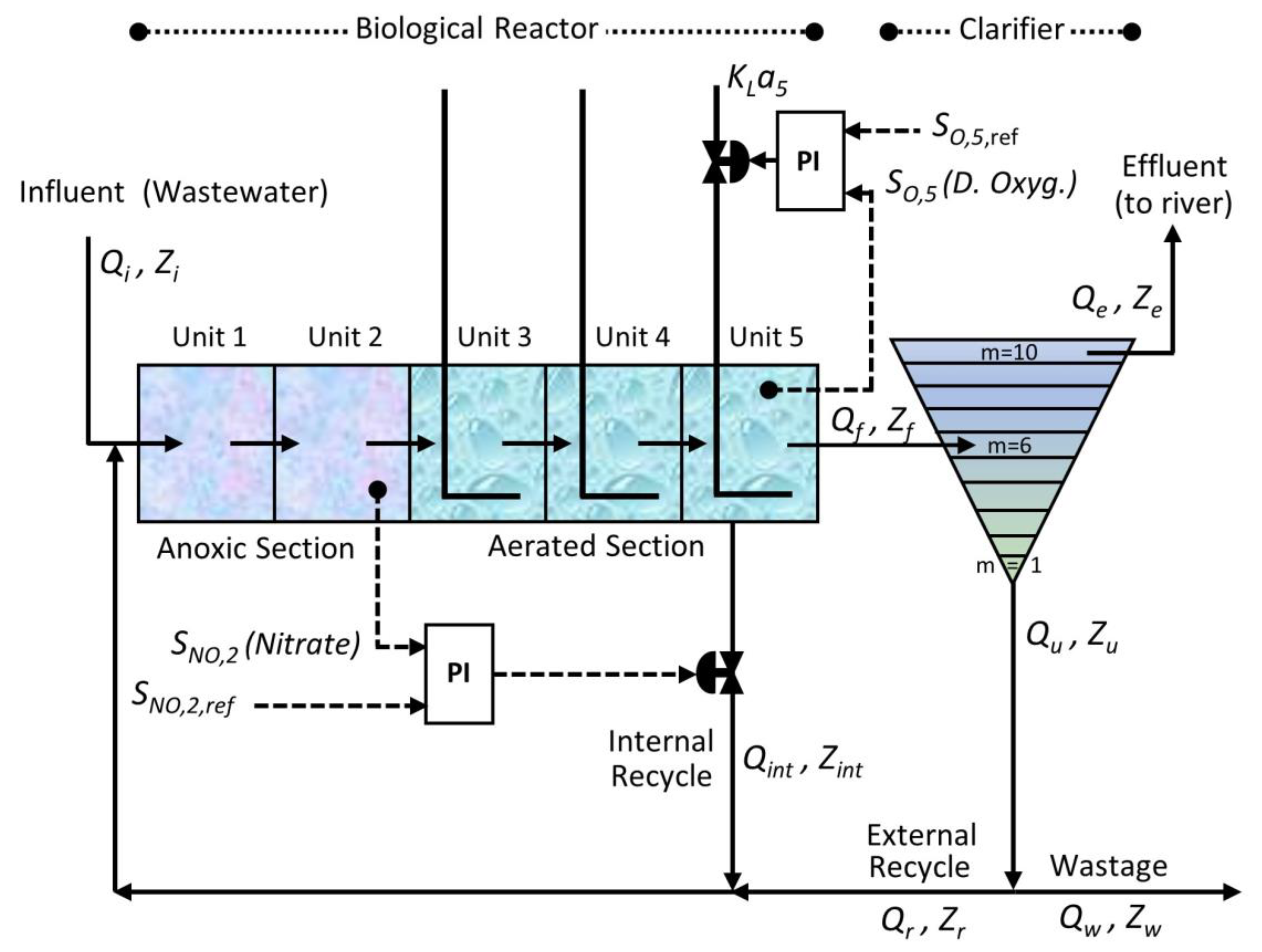
Figure 2.
FMBPC/CLP mixed strategy: implementation scheme.
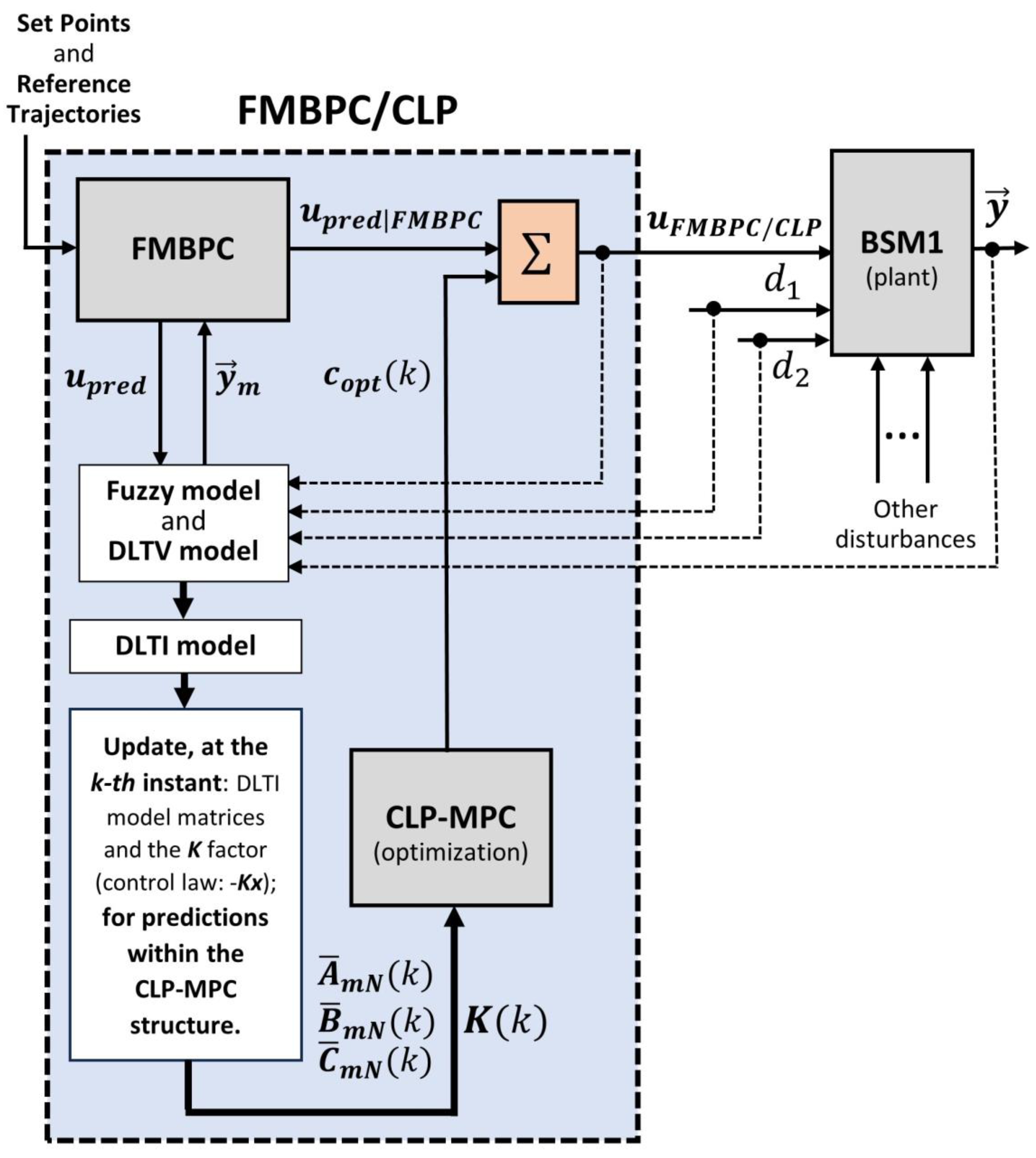
Figure 3.
Alternative control configuration for the BSM1 benchmark: variables SNO,2 and SNH,5 controlled by the FMBPC/CLP multivariable strategy and variable SO,5 controlled by a PI controller.
Figure 3.
Alternative control configuration for the BSM1 benchmark: variables SNO,2 and SNH,5 controlled by the FMBPC/CLP multivariable strategy and variable SO,5 controlled by a PI controller.
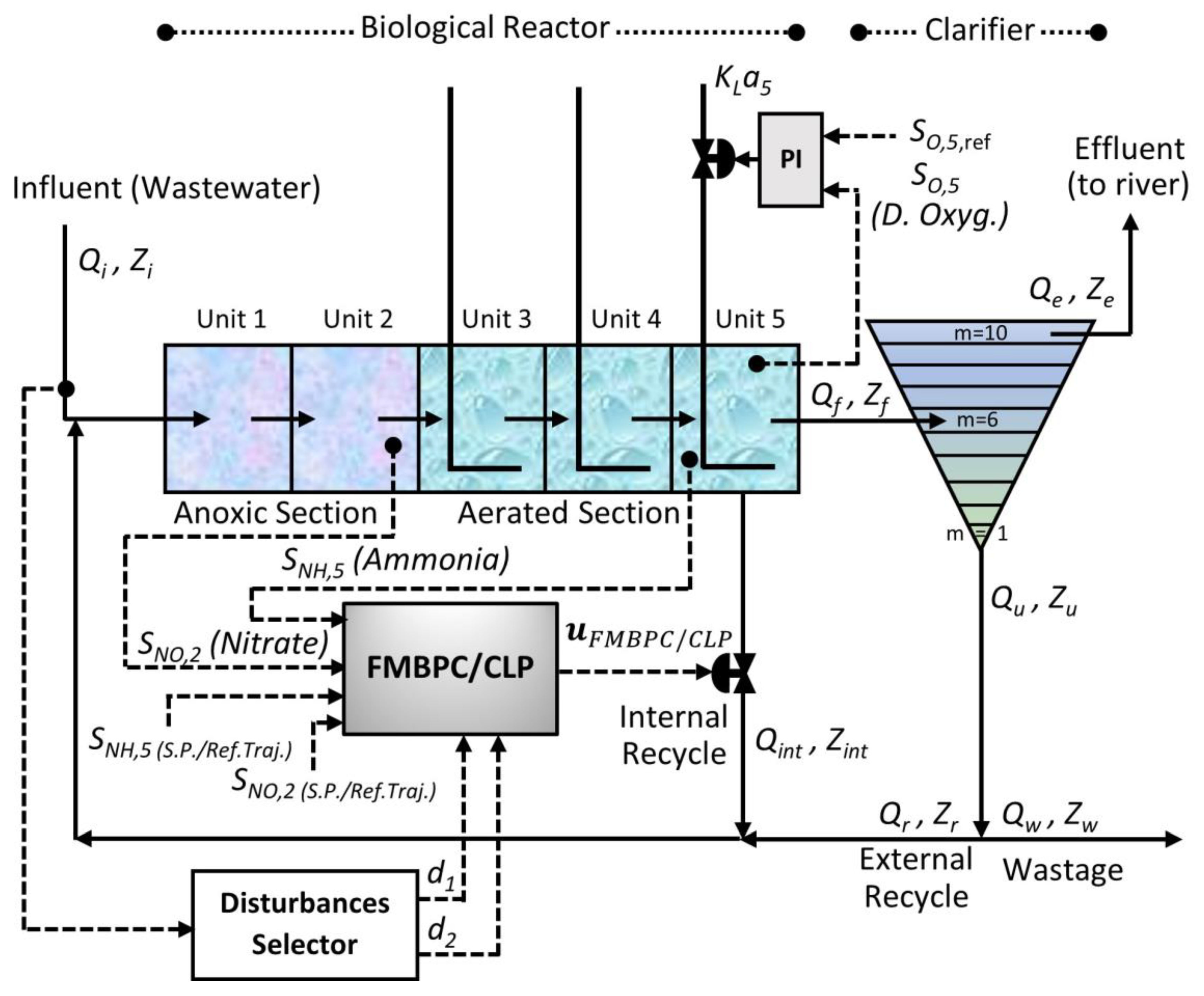
Figure 4.
BSM1 plant model (open loop).
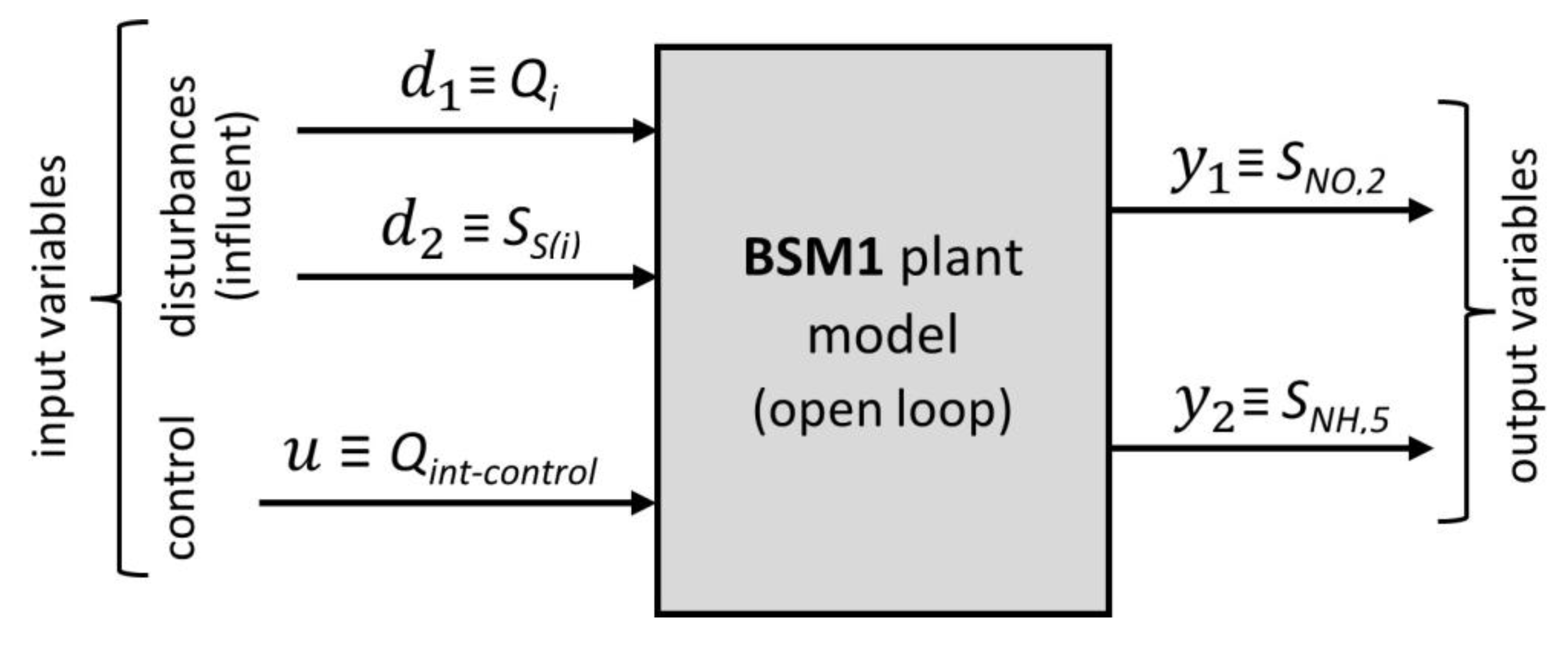
Figure 5.
Open-loop configuration for obtaining input-output data for the BSM1 benchmark.
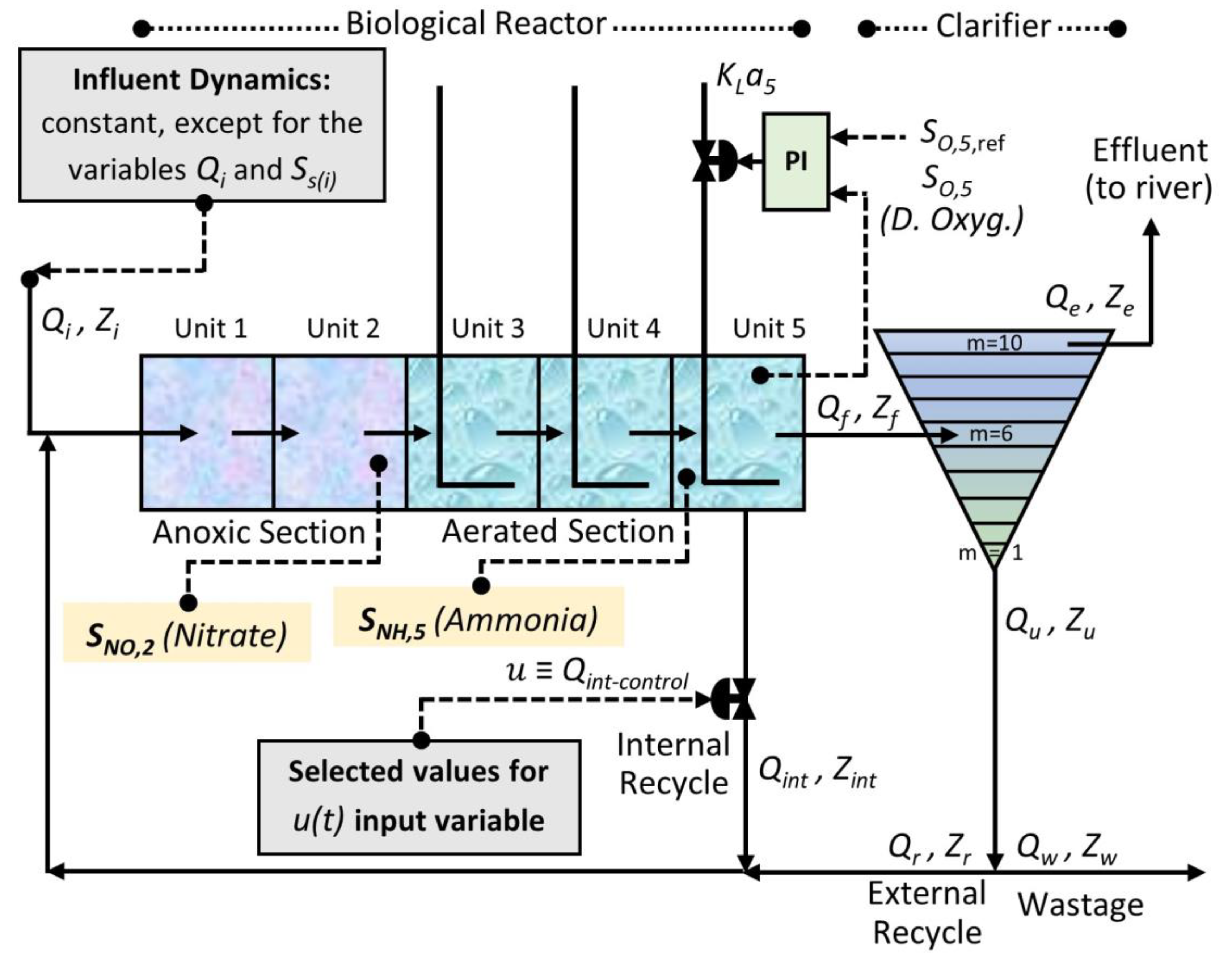
Figure 6.
Numerical input-output data used for identification of fuzzy model: input data.
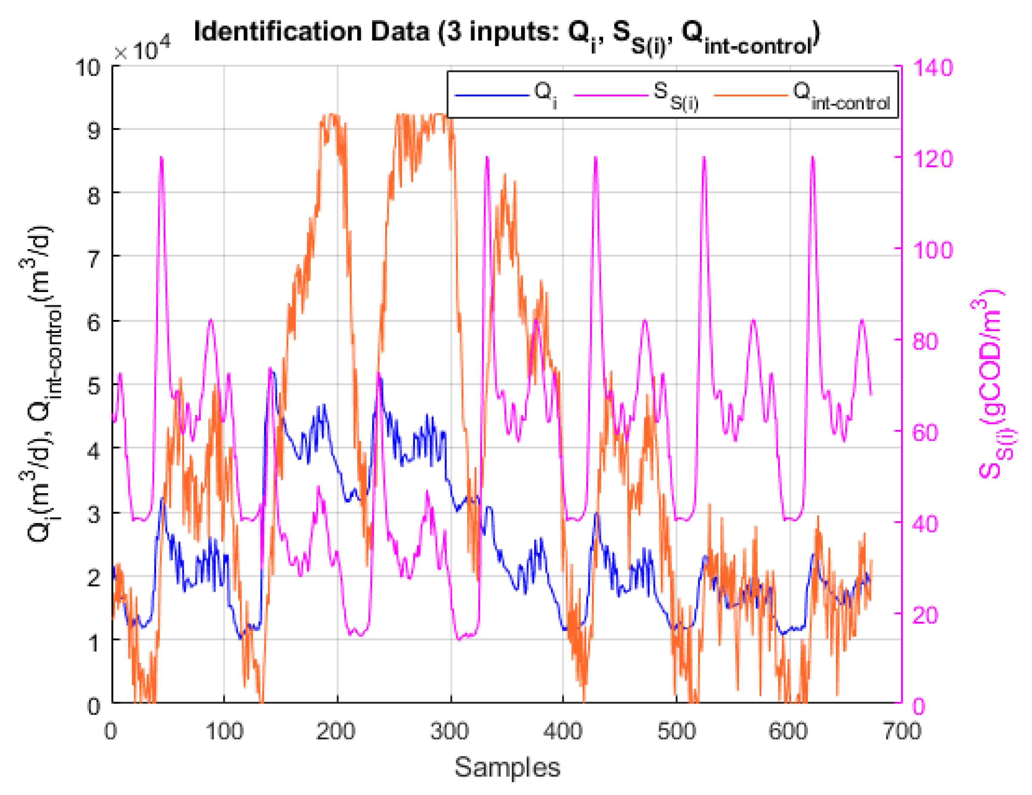
Figure 7.
Numerical input-output data used for identification of fuzzy model: output data.
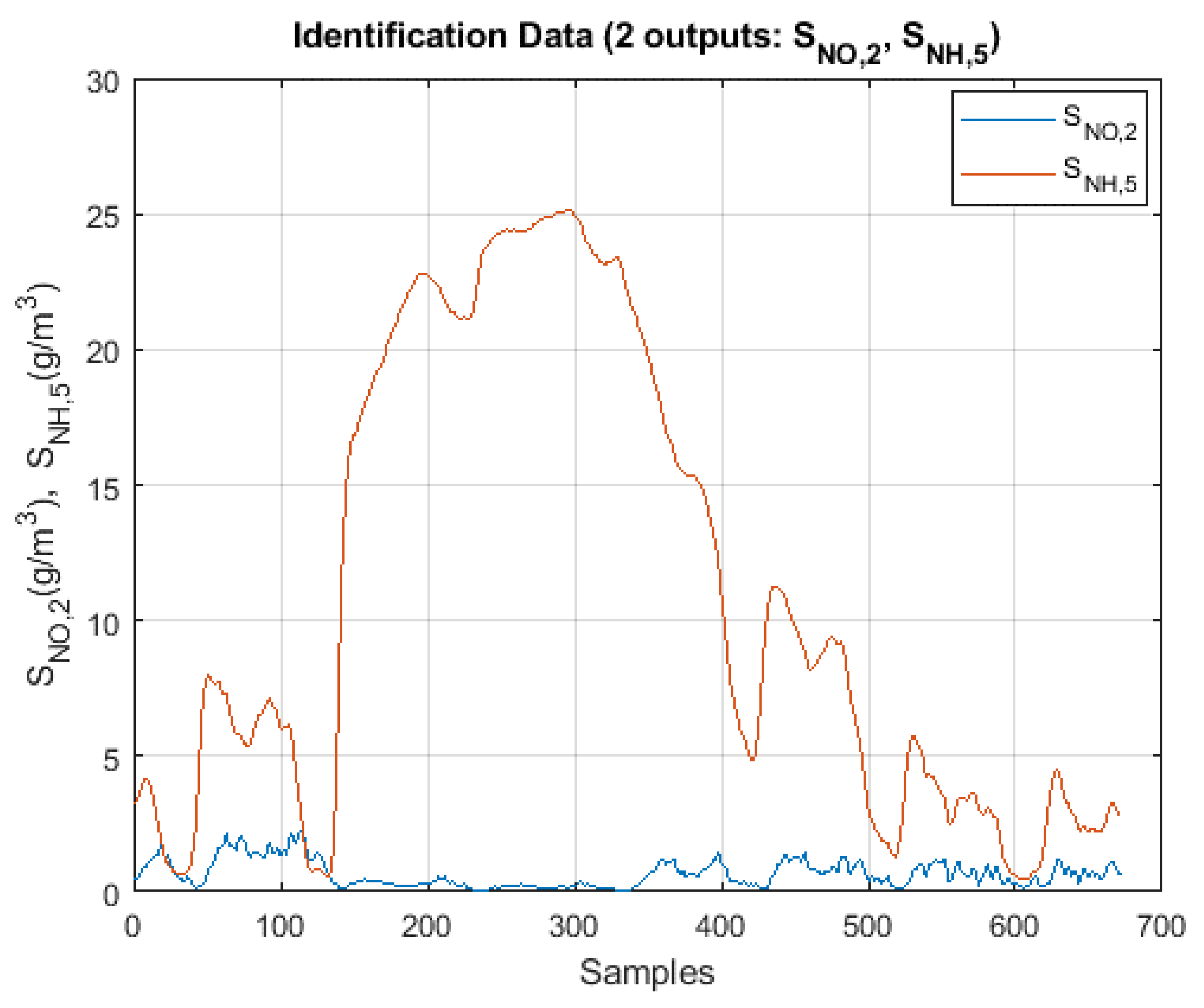
Figure 10.
Case 1a: Rain weather. SNO,2 (Nitrate) and SNH,5 (Ammonia) controlled by FMBPC/CLP strategy. Data recording time interval: 7th to 14th day.
Figure 10.
Case 1a: Rain weather. SNO,2 (Nitrate) and SNH,5 (Ammonia) controlled by FMBPC/CLP strategy. Data recording time interval: 7th to 14th day.
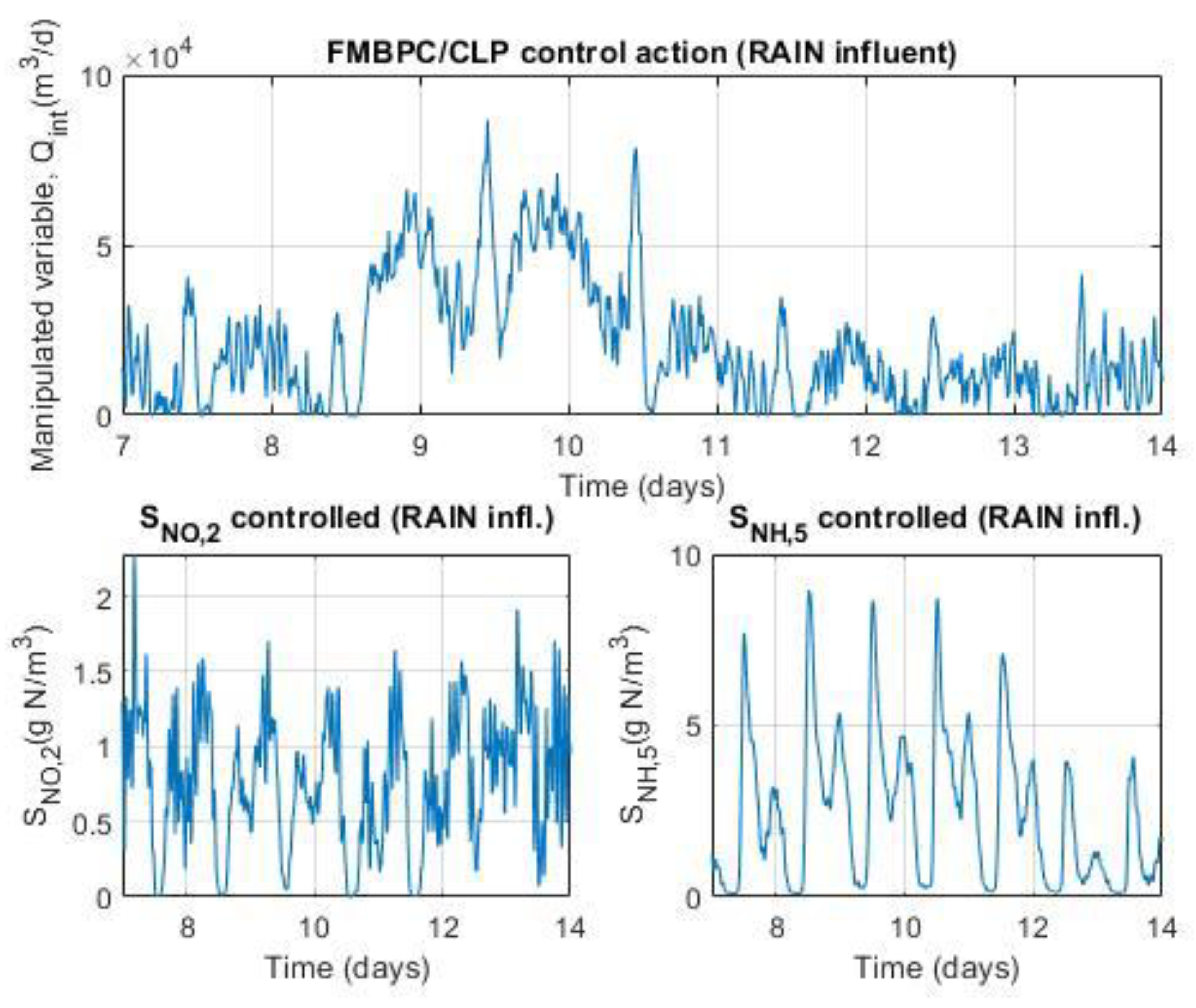
Figure 11.
Case 1b: Rain weather. SNO,2 (Nitrate) controlled by PID strategy. Data recording time interval: 7th to 14th day.
Figure 11.
Case 1b: Rain weather. SNO,2 (Nitrate) controlled by PID strategy. Data recording time interval: 7th to 14th day.
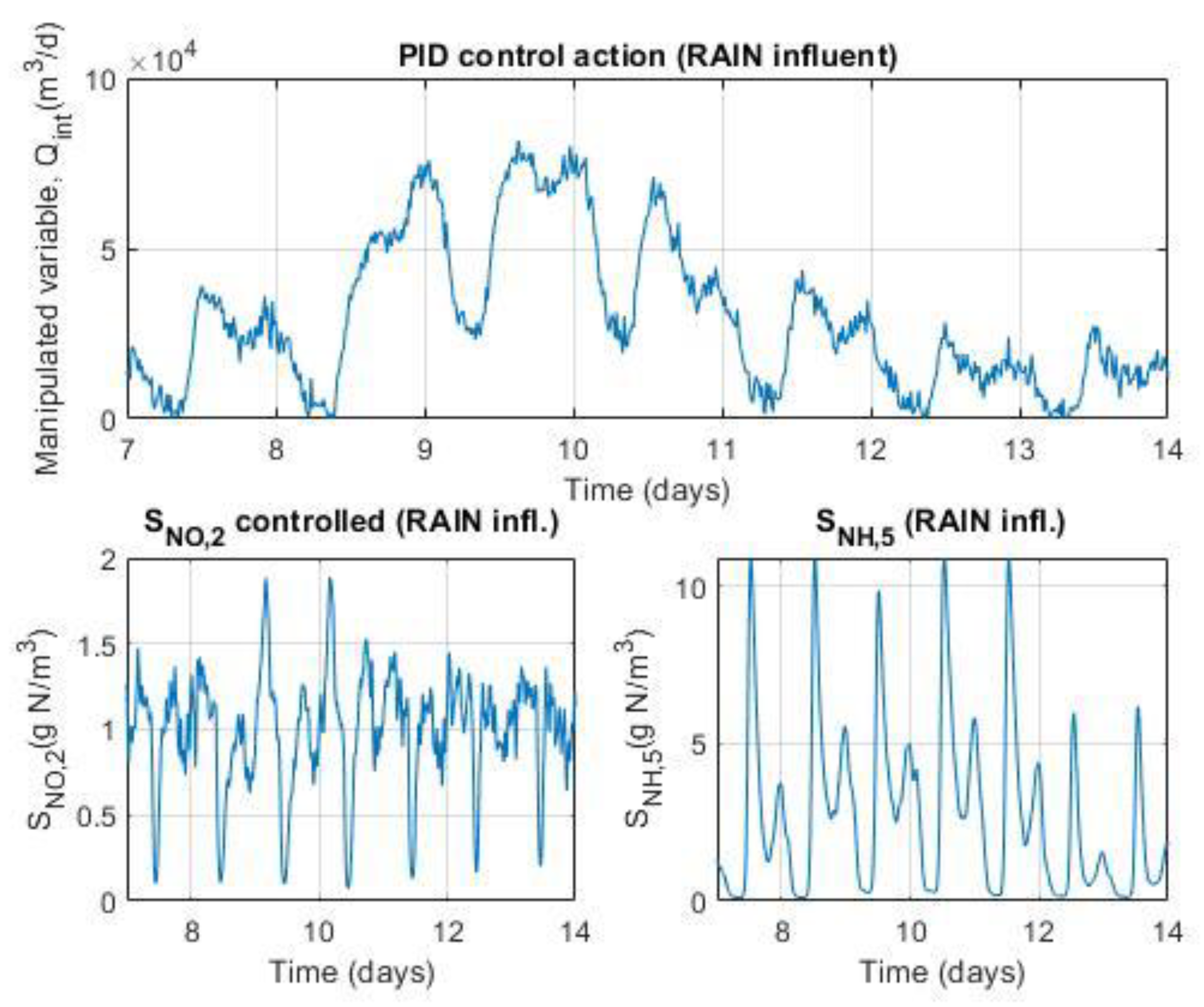
Figure 12.
Case 1c: Dry weather. SNO,2 (Nitrate) and SNH,5 (Ammonia) controlled by FMBPC/CLP strategy. Data recording time interval: 7th to 14th day.
Figure 12.
Case 1c: Dry weather. SNO,2 (Nitrate) and SNH,5 (Ammonia) controlled by FMBPC/CLP strategy. Data recording time interval: 7th to 14th day.
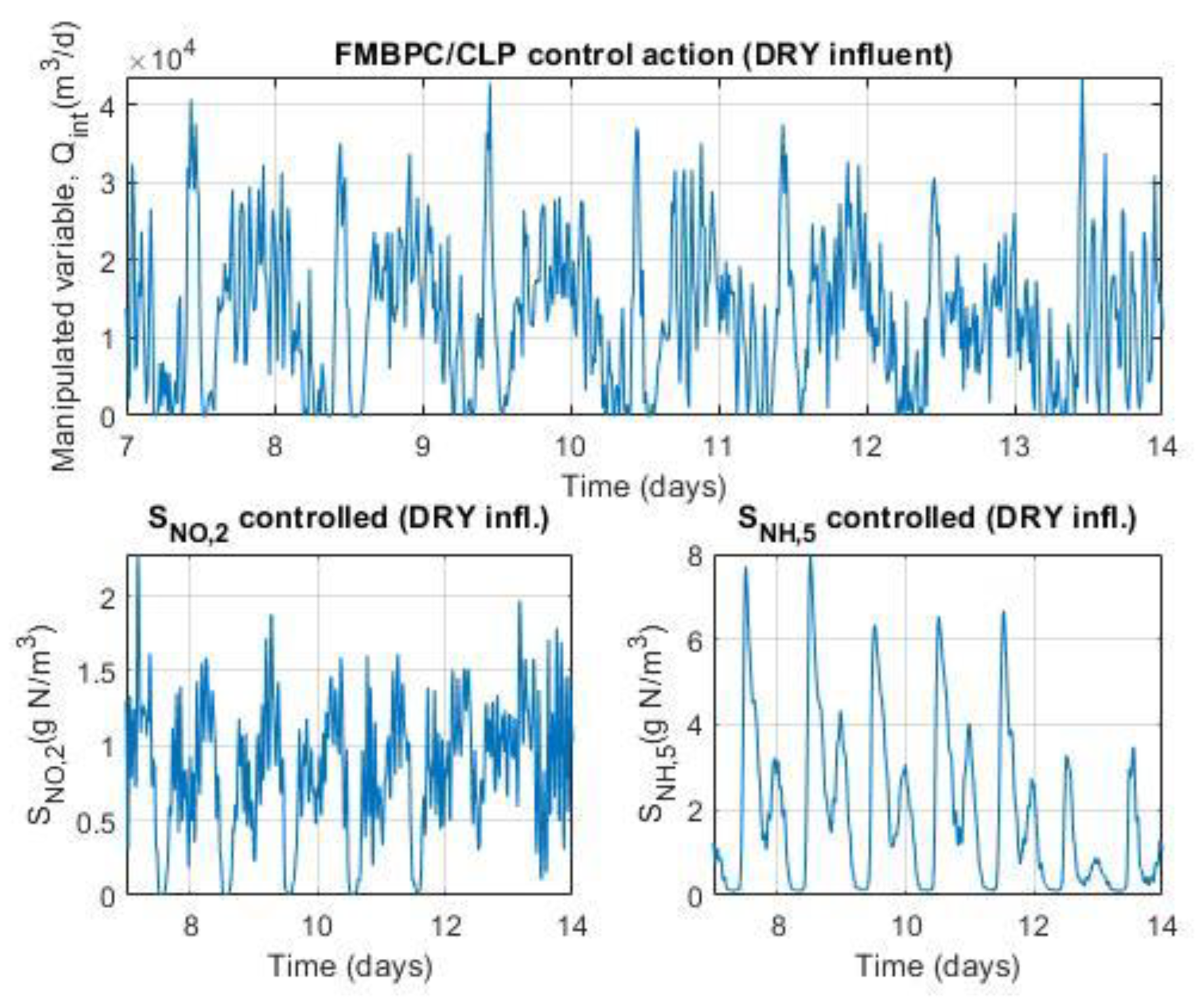
Figure 13.
Case 1d: Storm weather. SNO,2 (Nitrate) and SNH,5 (Ammonia) controlled by FMBPC/CLP strategy. Data recording time interval: 7th to 14th day.
Figure 13.
Case 1d: Storm weather. SNO,2 (Nitrate) and SNH,5 (Ammonia) controlled by FMBPC/CLP strategy. Data recording time interval: 7th to 14th day.
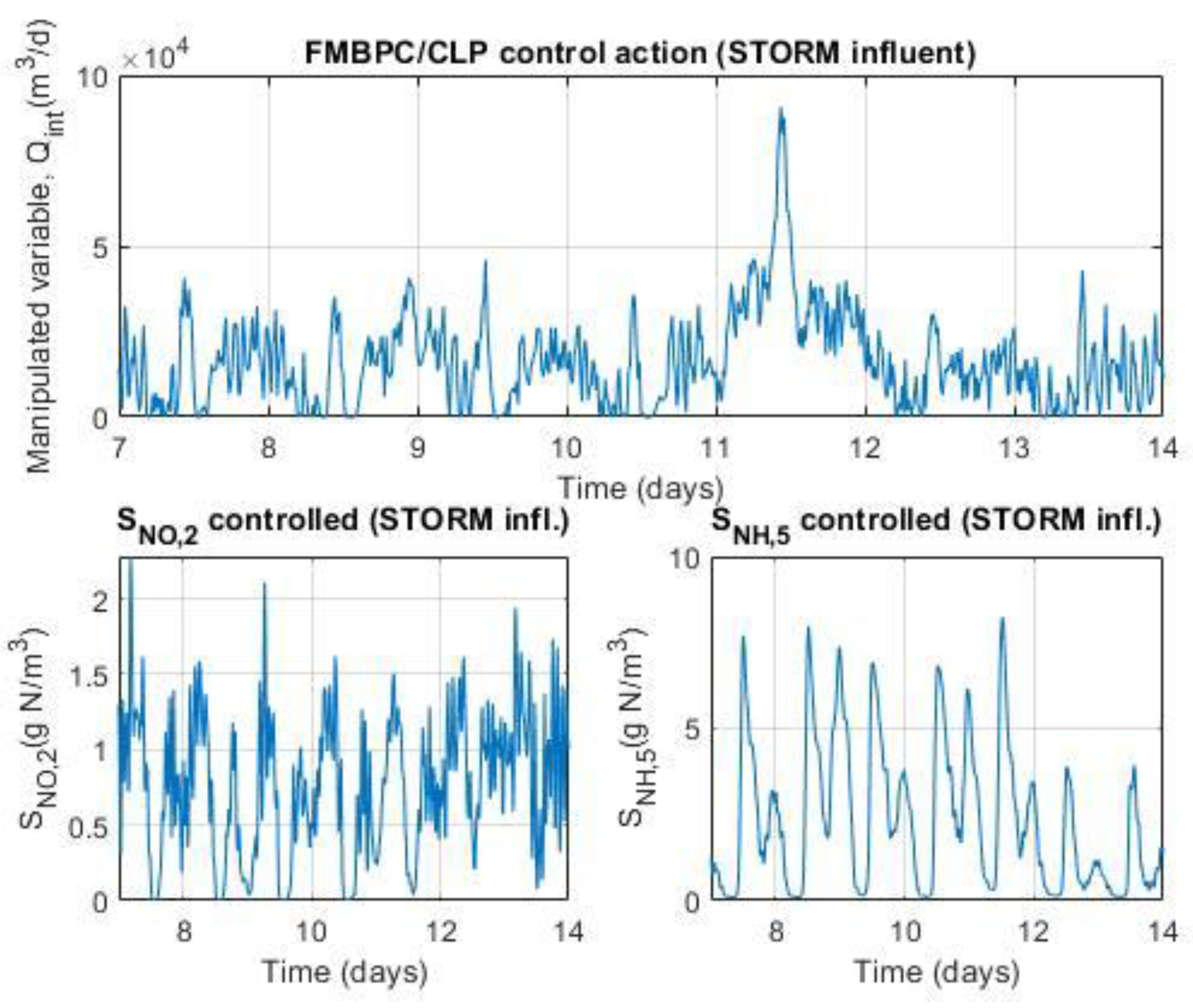
Figure 14.
Case 2a: Rain weather. SNO,2 (Nitrate) and SNH,5 (Ammonia) controlled by FMBPC/CLP strategy. (). Time interval: 7th to 14th day.
Figure 14.
Case 2a: Rain weather. SNO,2 (Nitrate) and SNH,5 (Ammonia) controlled by FMBPC/CLP strategy. (). Time interval: 7th to 14th day.
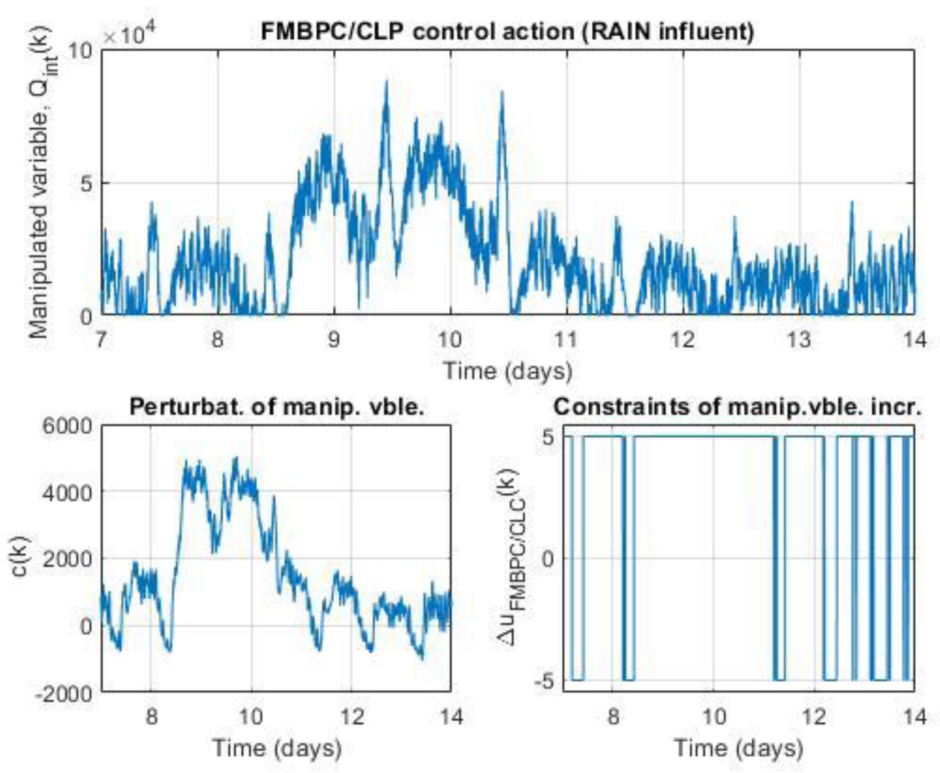
Figure 15.
Case 2b: Rain weather. SNO,2 (Nitrate) and SNH,5 (Ammonia) controlled by FMBPC/CLP strategy. (). Time interval: 7th to 14th day.
Figure 15.
Case 2b: Rain weather. SNO,2 (Nitrate) and SNH,5 (Ammonia) controlled by FMBPC/CLP strategy. (). Time interval: 7th to 14th day.
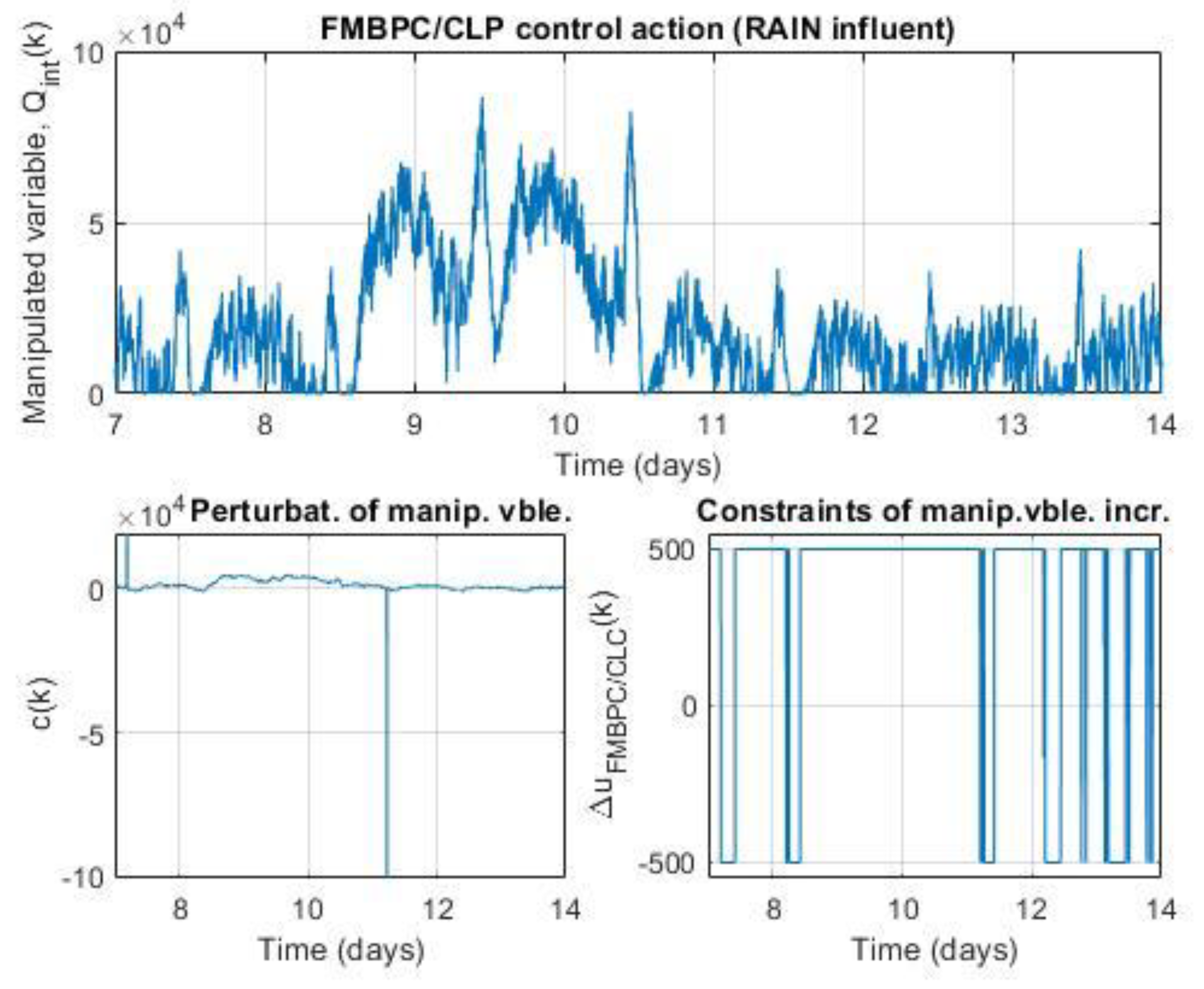
Figure 16.
Case 2c: Rain weather. SNO,2 (Nitrate) and SNH,5 (Ammonia) controlled by FMBPC/CLP strategy. (). Time interval: 7th to 14th day.
Figure 16.
Case 2c: Rain weather. SNO,2 (Nitrate) and SNH,5 (Ammonia) controlled by FMBPC/CLP strategy. (). Time interval: 7th to 14th day.
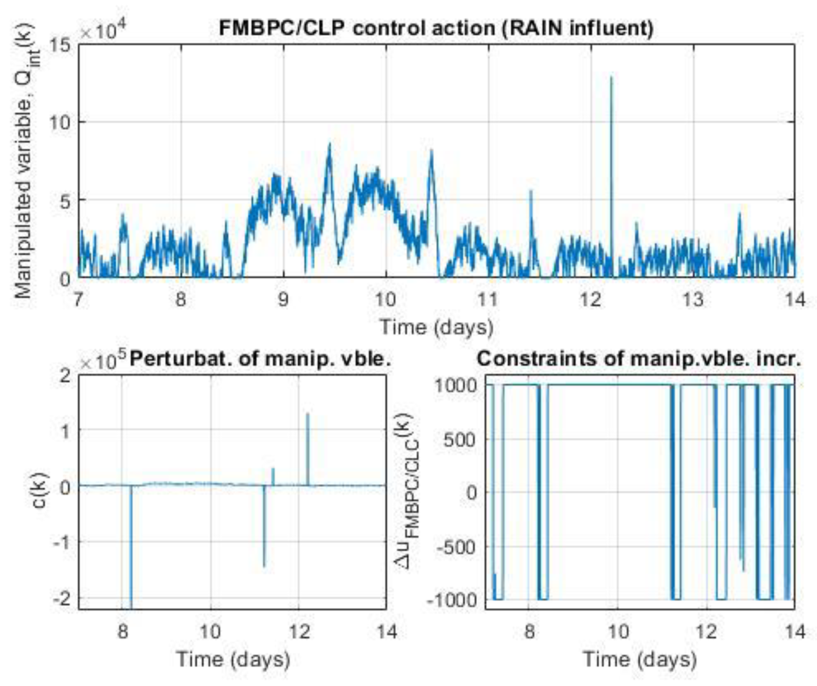
Figure 8.
Validation of the chosen fuzzy base-model (includes VAF indices).
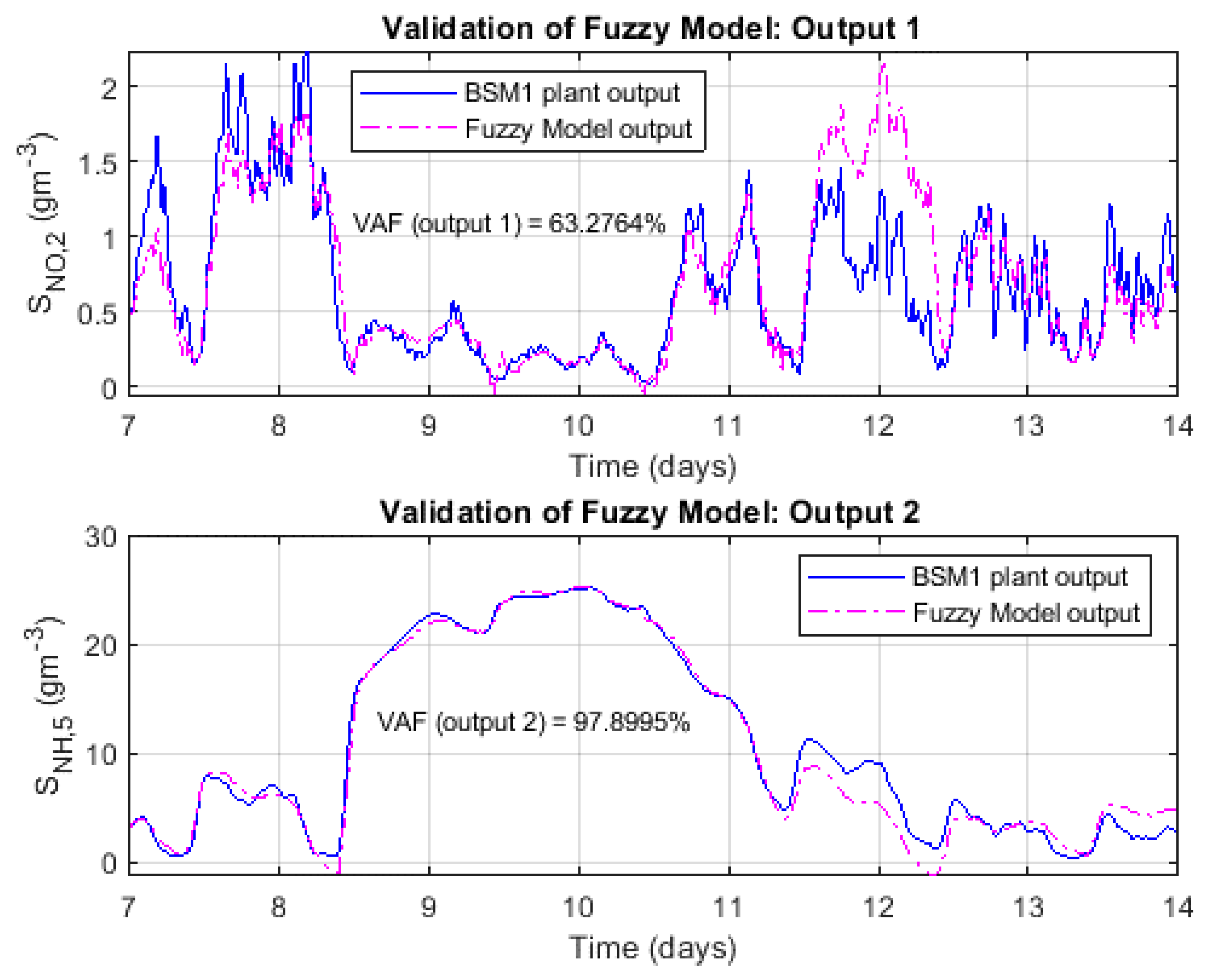
Figure 9.
Validation of the second fuzzy model (includes VAF indices).
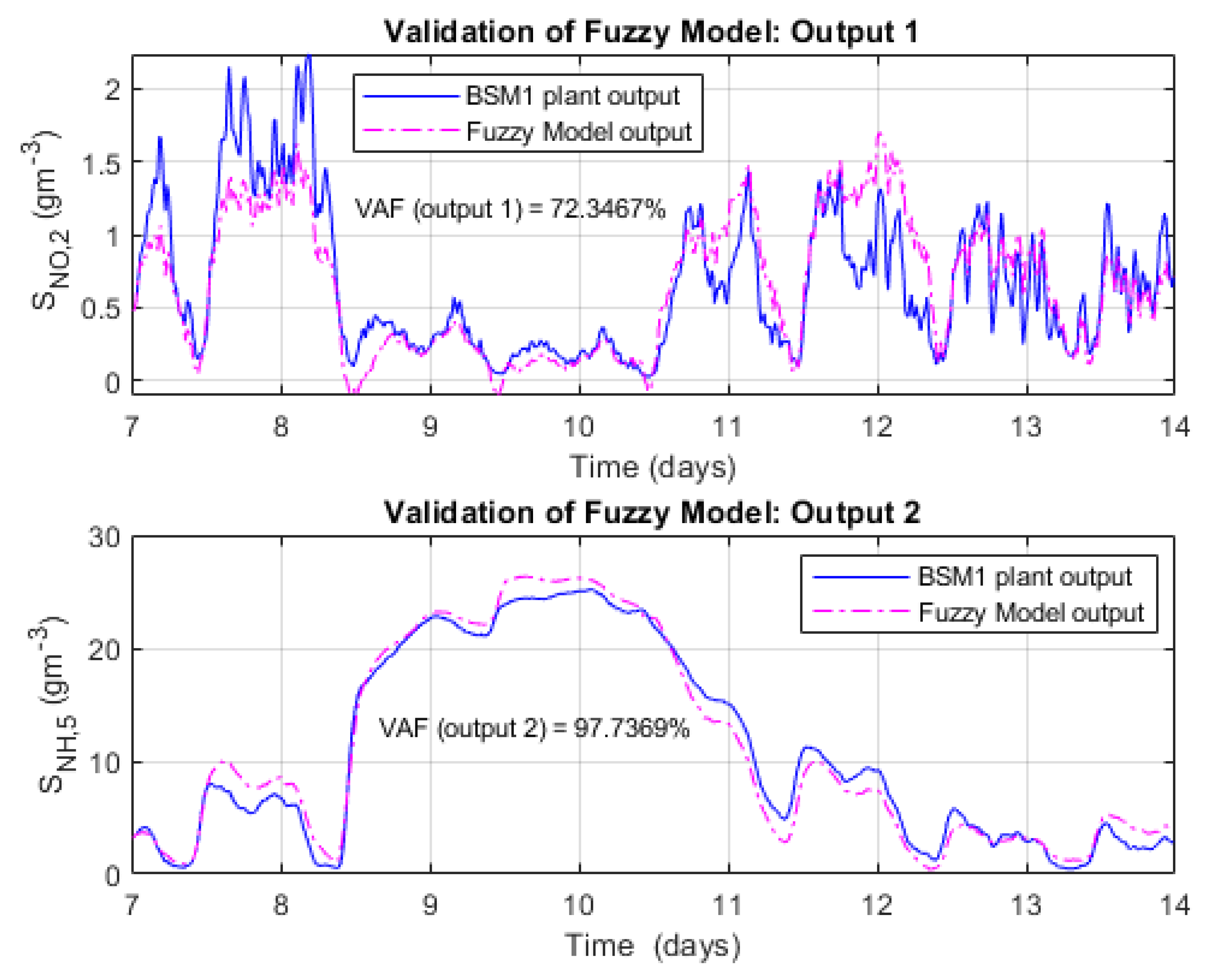

Table 1.
Alternative control configuration for the BSM1 benchmark: control loops.
| Control loop -controlled variables- (reactor unit no.) |
Control algorithm |
Input variables to the controller |
Control variables |
Manipulated variables |
|
Oxygen Control Loop SO,5 (5th unit) |
PI | SO,5 (measure) | PI output | KLa5 |
| SO,5,ref | ||||
|
Nitrate and Ammonia Control Loop SNO,2 (2nd unit) y SNH,5 (5th unit) |
FMBPC/CLP | SNO,2 (measure) | Qint | |
| SNH,5 (measure) | ||||
| SNO,2 (S.P. / Ref.Traj.) | ||||
| SNH,5 (S.P. / Ref.Traj.) | ||||
| d1 ≡ Qi | ||||
| d2 ≡ SS(i) |
Table 2.
List of variables characteristic of the influent (influent data).
| Variables | Description |
| Soluble inert organic matter | |
| Readily biodegradable substrate | |
| Particulate inert organic matter | |
| Slowly biodegradable substrate | |
| Active heterotrophic biomass | |
| Active autotrophic biomass | |
| Particulate products arising from biomass decay | |
| Oxygen | |
| Nitrate and nitrite nitrogen | |
| NH4+ + NH3 nitrogen | |
| Soluble biodegradable organic nitrogen | |
| Particulate biodegradable organic nitrogen | |
| Alkalinity | |
| Influent flow rate |
Table 3.
Plant input and output variables (BSM1 benchmark).
| Input/Output (role) |
Generic notation |
Physicochemical notation |
Description |
| Input 1 of 3 (disturbance) | Influent flow rate at the plant inlet | ||
| Input 2 of 3 (disturbance) | Concentration of readily biodegradable substrate in the influent | ||
| Input 3 of 3 (control) | Control of internal recirculation flow rate | ||
| Output 1 of 2 | Nitrate concentration in the second reactor unit | ||
| Output 2 of 2 | Ammonia concentration in the fifth reactor unit |
Table 4.
Structural parameters of BSM1 benchmark fuzzy identification (chosen configuration).
| Parameter | Values | Meaning (dynamics of the recursive model) |
|
: 4 data clusters ⇒ 4 rules : 3 data clusters ⇒ 3 rules |
||
| (Row 1) → depends on: {, } (Row 2) → depends on: {, } |
||
| (Row 1) → depends on: {, , , } (Row 2) → depends on: {, , , } |
||
| (Row 1) → inputs , , e each have one transport delay with respect to output (Row 2) → inputs , , e each have one transport delay with respect to output |
||
| Sample time (days) |
where:
: number of data clusters (for each output)
: output-output dynamic relationship
: input-output dynamic relationship
: input-output transport delays
: sample time (days)
: -ésimo time instant (days)
: -th plant input, at the -th time instant ()
: -th plant output, at the -th time instant
Table 5.
Composition of the antecedent-consequent vector () of each of the two outputs (configuration chosen for the identification of the BSM1 benchmark).
Table 5.
Composition of the antecedent-consequent vector () of each of the two outputs (configuration chosen for the identification of the BSM1 benchmark).
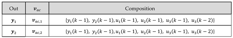 |
Table 11.
Effluent average concentrations (flow-weighted) and limit-values , during the final seven days, for the PID and FMBPC/CLP strategies (rain weather).
Table 11.
Effluent average concentrations (flow-weighted) and limit-values , during the final seven days, for the PID and FMBPC/CLP strategies (rain weather).
|
Control
Strategy |
Ammonia
(SNH) < 4 mg N/l (g N/m3) |
Total Nitrogen
(TN) < 18 mg N/l (g N/m3) |
Suspended Solids
(TSS) < 30 mg SS/l (g SS/m3) |
BOD5 < 10 mg BOD/l (g BOD/m3) |
CODtotal < 100 mg COD/l (g COD/m3) |
| FMBPC/CLP | 2.99 | 15.43 | 16.18 | 3.46 | 45.45 |
| PID | 3.23 | 14.75 | 16.18 | 3.46 | 45.43 |
Table 12.
Violation of limits of SNH and TN in the effluent, during the final seven days, for the PID and FMBPC/CLP strategies (rain weather).
Table 12.
Violation of limits of SNH and TN in the effluent, during the final seven days, for the PID and FMBPC/CLP strategies (rain weather).
|
Control
Strategy |
Ammonia Nitrogen (SNH) maximum level
violations → Limit: 4 mg N/l ( ≡ 4 g N/m3) |
Total Nitrogen (TN) maximum level
violations → Limit: 18 mg N/l ( ≡ 18 g N/m3) |
||
| number of days (%) | number of different occasions | number of days (%) | number of different occasions | |
| FMBPC/CLP | 1.78 (25.45%) | 8 | 2.04 (29.17%) | 9 |
| PID | 1.90 (27.08%) | 8 | 0.77 (11.01%) | 5 |
Table 13.
95th percentile of SNH, TN and TSS concentrations in the effluent, during the final seven days, for the PID and FMBPC/CLP strategies (rain weather).
Table 13.
95th percentile of SNH, TN and TSS concentrations in the effluent, during the final seven days, for the PID and FMBPC/CLP strategies (rain weather).
|
Control
Strategy |
Ammonia95
→ 95th percentile of SNH (mg N/l ≡ g N/m3) |
TN95
→ 95th percentile of TN (mg N/l ≡ g N/m3) |
TSS95
→ 95th percentile of TSS (mg SS/l ≡ g SS/m3) |
| FMBPC/CLP | 6.05 | 20.62 | 21.68 |
| PID | 8.04 | 19.14 | 21.70 |
Table 14.
Other effluent quality variables, during the final seven days, for the PID and FMBPC/CLP strategies (rain weather).
Table 14.
Other effluent quality variables, during the final seven days, for the PID and FMBPC/CLP strategies (rain weather).
|
Control
Strategy |
Effluent quality index
EQI (kg poll.units/day) |
Average aeration energy per day
AE (kWh/day) |
Average pumping energy per day
PE (kWh/day) |
Total operational cost Index
OCI |
| FMBPC/CLP | 8240.22 | 7203.75 | 1576.13 | 15970.64 |
| PID | 8184.73 | 7170.74 | 1937.70 | 15984.55 |
Table 15.
Performance assessment of controllers, FMBPC/CLP and PID, according to ISE and IAE criteria (rainy weather).
Table 15.
Performance assessment of controllers, FMBPC/CLP and PID, according to ISE and IAE criteria (rainy weather).
|
Control
Strategy |
Integral of square error (ISE) | Integral of absolute error (IAE) | ||
| Control of SNO,2 | Control of SNH,5 | Control of SNO,2 | Control of SNH,5 | |
| FMBPC/CLP | 1.79 | 55.97 | 2.88 | 14.30 |
| PID | 0.79 | Not controlled | 1.73 | Not controlled |
Table 6.
Takagi-Sugeno type fuzzy model for the output.
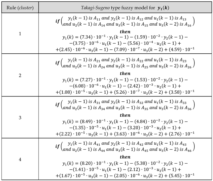 |
where:
: fuzzy set (or fuzzy value) associated with the component of the antecedent vector, for the rule (), characterized by a certain membership function, ().
Table 7.
Takagi-Sugeno type fuzzy model for the output.
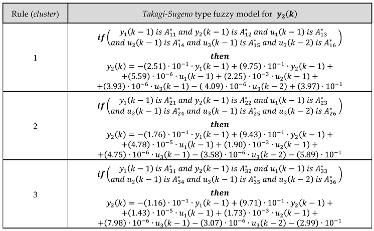 |
where:
: fuzzy set (or fuzzy value) associated with the component of the antecedent vector, for the rule (), characterized by a certain membership function, ().
Table 8.
Structural parameters of the fuzzy identification of a second model (with more complex dynamics).
Table 8.
Structural parameters of the fuzzy identification of a second model (with more complex dynamics).
| Parameter | |||||
| Values |
Table 9.
Setting of the first group of control experiments with the BSM1 benchmark.
| Influent data (weather type) | Case | Control loop and controlled variables (react. unit) |
Control Algorithm (manipulate variable) |
Control strategy parameters |
Simulation parameters | ||
| Set Point | Simul. interval | ||||||
| Rain weather | 1a |
Oxygen SO,5 (5th u.) |
PI1 (KLa5) | K = 25 | SO,5|s.p. = 2 | 0 to 14 (days) | |
| Ti = 0.002 | |||||||
| Tt = 0.001 | |||||||
|
Nitrate & Ammonia SNO,2 (2nd u.) SNH,5 (5th u.) |
FMBPC/CLP (Qint) | FMBPC | Fuzzy Model: FM |
SNO,2|s.p. = 1 SNH,5|s.p.= 0.67 |
|||
| ar1 = 0.76 | |||||||
| ar2 = 0.96 | |||||||
| H = 25 | |||||||
| CLP | Q1 = 1 | ||||||
| Q2 = 1 | |||||||
| R = 1 | |||||||
| nc = 42 (steps) | |||||||
| |Δu|máx = 5 | |||||||
| 1b |
Oxygen SO,5 (5th u.) |
PI1 (KLa5) | K = 25 | SO,5|s.p. = 2 | |||
| Ti = 0.002 | |||||||
| Tt = 0.001 | |||||||
|
Nitrate SNO,2 (2nd u.) |
PI2 (Qint) | K = 104 | SNO,2|s.p. = 1 | ||||
| Ti = 0.025 | |||||||
| Tt = 0.015 | |||||||
| Dry weather | 1c | Same specifications as in Case 1a (control strategy for the variables Nitrate & Ammonia: FMBPC/CLP) | |||||
| Storm weather | 1d | Same specifications as in Case 1a (control strategy for the variables Nitrate & Ammonia: FMBPC/CLP) | |||||
Table 10.
Setting of the second group of control experiments with the BSM1 benchmark. Handling constraints with the FMBPC/CLP strategy.
Table 10.
Setting of the second group of control experiments with the BSM1 benchmark. Handling constraints with the FMBPC/CLP strategy.
| Influent data (climate type) |
Case | Control loop and controlled variables (react. unit) |
Control algorithm (capable of handling constraints) |
Constraints |Δu|máx |
Simulation parameters | |
| Set Point | Simul. interval | |||||
| Rain weather | 2a |
Nitrate & Ammonia SNO,2 (2nd u.) SNH,5 (5th u.) |
FMBPC/CLP | |Δu|máx=5 |
SNO,2|s.p.=1 SNH,5|s.p.= 0.67 |
0 to 14 (days) |
| 2b | -ídem- | -ídem- | |Δu|máx=500 | -ídem- | ||
| 2c | -ídem- | -ídem- | |Δu|máx=1000 | -ídem- | ||
where: all abbreviations, expressions, and units are the same as corresponding of the Table 9.
Disclaimer/Publisher’s Note: The statements, opinions and data contained in all publications are solely those of the individual author(s) and contributor(s) and not of MDPI and/or the editor(s). MDPI and/or the editor(s) disclaim responsibility for any injury to people or property resulting from any ideas, methods, instructions or products referred to in the content. |
© 2025 by the authors. Licensee MDPI, Basel, Switzerland. This article is an open access article distributed under the terms and conditions of the Creative Commons Attribution (CC BY) license (https://creativecommons.org/licenses/by/4.0/).
Copyright: This open access article is published under a Creative Commons CC BY 4.0 license, which permit the free download, distribution, and reuse, provided that the author and preprint are cited in any reuse.


