Submitted:
18 November 2025
Posted:
19 November 2025
You are already at the latest version
Abstract
Optimal Order Execution is a well-established problem in finance that pertains to the flawless execution of a trade (buy or sell) for a given volume within a specified time frame. This problem revolves around optimizing returns while minimizing risk, yet recent research predominantly focuses on addressing one aspect of this challenge. In this paper, we introduce an innovative approach to Optimal Order Execution within the US market, leveraging Deep Reinforcement Learning (DRL) to effectively address this optimization problem holistically. Our study assesses the performance of our model in comparison to two widely employed execution strategies: Volume Weighted Average Price (VWAP) and Time Weighted Average Price (TWAP). Our experimental findings clearly demonstrate that our DRL-based approach outperforms both VWAP and TWAP in terms of return on investment and risk management. The model's ability to adapt dynamically to market conditions, even during periods of market stress, underscores its promise as a robust solution.
Keywords:
Optimum Order Execution
; Deep Reinforcement Learning
; TWAP
; VWAP
; returns
; risks
CCS CONCEPTS
•Computer systems organization Embedded systems → Embedded systems → Redundancy; Robotics; •Networks → Network reliability.
1. Introduction
Optimal order execution addresses a fundamental question within the realm of finance: when a trader possesses a volume denoted as V of one or multiple financial instruments and intends to execute trades (buy or sell) within a specified time horizon T, what strategy should be employed to maximize returns while minimizing risk? The timeframe T can vary from minutes to hours, days, months, or even years, contingent upon the investment horizon and other constraints at play. In most cases, this problem is approached as an intraday trading challenge, typically encompassing a single trading day. The central concept revolves around acquiring or purchasing a designated volume of an asset, such as a stock, at a favorable price point and subsequently selling or liquidating all or a portion of that volume when its price rises. This strategic maneuver results in profit for the trader. The problem formulation has many applications in liquidation or acquirement of a volume [9]. In this work, we focus on the liquidation of V volume aspect of the problem; we also discuss how the proposed methodology can be extended to the acquirement problem.
The simultaneous execution of multiple assets also intersects with the domain of Portfolio Management [6], a discipline concerned with the selection and management of a variety of assets to achieve long-term financial gains. Portfolio Management primarily revolves around the question of which assets to include in a portfolio for optimal performance. It is important to clarify that this paper’s focus does not extend to the realm of Portfolio Management. Instead, our scope is limited to the assumption that the portfolio comprises only a single asset, and our objective is to determine the ideal execution strategy for this specific asset. In our analysis, executions occur at one-minute intervals within the trading hours of the day, spanning from 9:30 AM to 4:00 PM, New York City Time, encompassing a total of 390 trading minutes. It is worth noting that during certain intervals within this timeframe, traders have the discretion to abstain from executing trades or selling any portion of the volume (hold), opting to retain their positions.
Order execution, as previously discussed, constitutes an optimization problem between Return and Risk. Specifically, it involves the delicate equilibrium between ’market impact,’ arising from the execution of a substantial trade volume within a short timeframe, and ’price risk,’ which is the potential for missed advantageous trading opportunities due to slow trading [9]. Within the designated time horizon T, there exist practically countless methods for executing an order. These approaches range from rapidly liquidating the entire volume, trading at a leisurely pace, to executing trades in a purely random manner. However, it is crucial to recognize that overly arbitrary trading strategies can lead to unfavorable outcomes, such as failing to meet the deadline for completing the order within the time horizon T or overlooking valuable market opportunities. Consequently, it becomes evident in this work that overly simplistic strategies, such as TWAP, are inherently flawed.
1.1. State of the Art
Some model-based solutions are adopted to tackle optimum order execution [1,2,4,8]. In these works, mathematical models are built using past market data to help traders predict the ideal trading volume at a given time for optimum order execution. However, these models often rely on strict assumptions about market behavior, such as linearity in permanent market impact and transaction costs. [3]. These models are significantly weak in different markets including a difficult market condition, otherwise called a Stressful Market Condition, and also for volatile markets, e.g., mid and small market capitalization (from now on, we will call it caps). Other simple yet famous and widely used models are TWAP (Time Weighted Average Price) and VWAP (Volume Weighted Average Price), which are discussed later in detail. However, these methods also take in strict assumptions making themselves weak in different markets.
Deep Reinforcement Learning (Deep RL) [26] combines deep learning [21,25,33] and reinforcement learning [23,38] principles to create self-learning algorithms that can make decisions by interacting with their environment. By using deep neural networks to interpret high-dimensional data, such as images or videos, Deep RL can handle complex tasks and large state spaces that traditional reinforcement learning methods struggle with. The model learns to map states to actions by receiving and maximizing rewards through trial and error, allowing it to adapt and optimize its behavior over time.
The success of Deep Reinforcement Learning is celebrated in different domains of research and industry. It is being applied in Economics [10], Autonomous Driving [11,13,24,34], games [29,41] , real world complexities [30], neuroscience research [37], etc. Superhuman-level accuracy is received for many of these applications. Because of its sequential decision-making skills, Deep Reinforcement Learning also is a favorable solution in optimum order execution.
In many publications, the order execution problem is called a ‘two-fold’ problem, where the goal is to fulfill the whole order within the time window as well as either maximizing the gain or minimizing the loss. However, they do not consider how to simultaneously achieve both maximize the gain and minimize the loss while fulfilling the whole order. The trade-off between risk and return is fundamental to finance, and ignoring this fact can lead to large inaccuracy from the real market.
In [40], Yamada et. al. worked on Tokyo Stock Exchange (TSE) for a span of 29 months to study the factors that cause a market impact. In [32], Nevmyvaka et. al. worked on a single but important aspect of the entire problem: the transaction price. In [18], Ghosh et. al. examined the goal of minimizing transaction costs, including the costs of legal decision-making.
In [31], Nevmyvaka et. al. used Reinforcement Learning in Optimum Order Execution on a large scale for the first time. They also worked on Deep-Q Learning [39] where the action space (here, action resembles the trade) is discrete. Thus, it can never fully imitate the real market where the trading volume can have any possible value. In [27] Lin et. al. worked on an end-to-end optimum trade execution framework with Policy Gradient Reinforcement Learning. However, their model was not robust enough and was outrun in performance by statistical models like TWAP and VWAP in some cases. They also failed to share how their model could behave for volatile assets, and they only worked on large caps market capitalization where the markets are much stable. Furthermore, their models are trained with only last minute of market data. In our work, we have trained our models with last 10 minutes of market data. The significance of this action is discussed later in this study.
In [14], a seminal work is done for goal based wealth management problems, which can be applied in Optimum Order Execution. However, here the time horizon usually is much longer - generally in years. Moreover, the work is done on G-Learning, which is a probabilistic extension of Q-Learning. As mentioned above, Q-Learning can never fully emulate the real market.
In [16] Fang et. al. worked on Order Execution using a more advanced Policy Gradient Method. The current work’s advanced Policy Gradient model is developed as in [16]. The work in [16] also introduced a penalty term in their Loss Equation in order to check the Risk involved under control. The current work’s Reward and Loss equations are also influenced by the work in [16]. However, unlike the current work which is also studied in stressful markets, the work in [16] never mentioned if it has been studied in volatile market conditions. Their work predates the Covid period and was studied in Chinese Stock Market. Our work also examines the models in stressful markets like Covid periods and Inflation+War (and also, downfall of Meta) in the US market. The models in our work are more robust than any other works that we came across. Furthermore, despite adding the penalty term in the loss equation, the work in [16] never shared how their models behaved to mitigate the risk- something which is studied and examined thoroughly in our study. Lastly, some big strategic differences are: unlike the work in [16], the current work takes last 10 minutes of market data for training. Also, the current work, despite developing stock-specific models, also considers other similar markets under consideration. For example, for the training of a model for AAPL, the market data for FB, AMZN, MSFT, IBM and goog are also fed into the model as inputs. Significance of these strategies is discussed later in the study.
1.2. A New Approach
In this subsection, the novel aspects of the present work is discussed. It is also briefly mentioned why the model generated from the present work is more efficient than the other state-of-the-art models.
1. As mentioned earlier, the models generated in the present study yield better results than any other models we came across,
2. The final goal of the present work is the execution of the entire order within the time horizon while simultaneously maintaining both high return and low risk.
3. Unlike other works, the models generated in the present work are tested not only for Large Caps, but also for Mid Caps, Small Caps and ETFs. Furthermore, whereas the other state-of-the-art models are majorly tested only in Normal market conditions, the present models are tested also in stressful market conditions. The returns yield from the present models are tested in 72 different market conditions: (6 Large Caps + 8 Mid Caps + 8 Small Caps + 2 ETFs) in 3 different market conditions. The market conditions include the stock market crash due to Covid-19 [20,28,35], a global inflation [19], and war in europe [5,12,17]. We also closely studied the effects of the plummeting price of FB stock price because of covid, pandemic, lawsuit against Meta (the parent company), etc.
Moreover, associated risks of the present models are tested in about 15 different market scenarios.
4. The present models are fed with the last 10 minutes of market information. The strategic advantage of it is in this way the models can grasp a better picture of the market. We found that feeding fewer minutes of the data can lead to inaccurate prediction of the market by the models, and feeding more minutes of the data can result in vanishing gradient and unnecessary complication in the training process.
5. The models are stock-specific. But while training a model for a particular stock, we also fed data of other relevant stocks into the model. For example, while training the model for AAPL (a Large Cap), we also fed data from MSFT, FB, IBM, goog and AMZN (other 5 Large Caps) into the model. There is a strategic advantage of this decision even though this makes the training and prediction more expensive. Looking at only a specific stock can lead to overfitting. For example, on a particular day a particular stock is facing a bull market whereas other relevant stocks are facing bear market. Training a model with market data from only the particular stock can lead to a false sense of market. However, training the same model with a cumulative market data from the particular stock and the relevant stocks can lead to a much better prediction of the market.
2. Problem Formulation
For simplicity in this work, it is assumed that the Time Window T is composed of discrete time-steps: . Each of these time-steps has a corresponding price of stock. Thus, there are prices of the stock: {}. Here, refers to the price of the stock at time . At this time-step t, the trader proposes to sell a volume which will be executed at time at a price .
The final goal is to have maximum revenue or return from this problem. Thus the objective can be written as,
where V is the total volume of shares or initial order volume.
One must remember, must not be too high. Quantitatively, should be significantly fewer than the corresponding rest of the market sale. Thus, the problem statement is extended to:
where V is the total volume of shares or initial order volume and is the total market sale volume at time t. And the task of the model is to find the values of .
3. Methods
In this work, 3 models are used and their results are compared. These models are:
1.TWAP or Time Weighted Average Price
2.VWAP or Volume Weighted Average Price
3.DRL or Deep Reinforcement Learning
3.1. TWAP
For TWAP, the entire Order is evenly distributed throughout the entire time window T. So, , where T = 390 in this problem. The is calculated as the TWAP price. The TWAP price at a time t is calculated as follows:
where are the High, Low and Close Prices respectively.
The final TWAP Price, that is the price at which the orders will be executed, is as follows:
However, TWAP is a model based method and can be largely presumptuous to impractical assumptions. For example, evenly distributing the entire Order throughout the day can lead to a poor execution. There are always minutes on a day when the price of the stock is much higher than average. Selling more stock than the v at these minutes can be lucrative. On the other hand, there are also minutes on the day when the price of the stock is lower than average. And it is better to sell less (or, even hold) at those minutes.
3.2. VWAP
VWAP method is more advanced and more complex than the TWAP method. The idea behind the VWAP method is very practical. It considers the volumetric weighted average of the price over the simple average of the price.
VWAP method distributes orders in proportion to the (empirically estimated) market transaction volume in order to keep the execution price closely tracking the market average price ground truth [16].
However, just like TWAP, VWAP is also model based and can be largely presumptuous to impractical assumptions. For example, as one has no way of knowing the future market data of the rest of the day, empirically estimating the proportion for VWAP can be erroneous.
3.3. DRL
The Deep Reinforcement Learning (DLR) method is a natural choice for this study because of its sequential decision-making properties. With its non-linearity and Universal Function Approximation capacity, a Deep Learning model can imitate the market, the relationship between the market and the trade, previous trades, etc. without impractical assumptions. Note that liquidity (defined as the measurement of the ease at which an asset can be bought/sold) is a multidimensional beast [36], and so is the market. One needs superhuman capability to consider and take into account all of the factors influencing liquidity and the market. Hence, Deep Learning is a favorable choice for this problem.
As shown in Figure 1, the 2 inputs are: (i) Public Variable, (ii) Private Variable. The public variable is a tuple of length 10 which includes the market information of the last 10 minutes of that specific day. The private variable is a combination of 2 tuples, each of length 10 which includes the last 10 trades made by our model on that specific day and the last 10 minutes of that specific day respectively. For the first 9 minutes of a day when one does not have the last 10 minutes of market information and last 10 trades, the tuples are made with the available market information or trades by the trader and some 0s to make them tuples of size 10 [22]. In the Inference Layer, the outputs of the LSTMs are concatenated. The action from the Actor sub-network of the Actor-Critic gives us information on what fraction of the original volume we need to sell now. So , where is the action at time t.
The LSTM component incorporates an initial CNN layer responsible for dimensionality reduction. It is subsequently followed by a Fully Connected Layer, an LSTM layer, and two final fully connected layers. The ReLU function serves as the nonlinearity employed. The Actor-Critic networks constitute a unified model consisting of multiple Fully Connected layers (ReLU is the nonlinear function utilized). The output of the last Fully Connected layer is inputted into both an actor head and a critic head. To obtain mu and sigma from the actor head, which are then employed to acquire the action sample from a Cauchy distribution, the sigmoid and softplus nonlinear functions are employed. In the critic head, a Fully Connected layer with an output size of 1 is employed to determine the State Value . The State Value reflects the present market state’s level of desirability. The learning rate used is 0.0001 and optimizer is Adam.
The Reward Function consists of 2 parts: positive reward and negative reward. The equation is:
here, denotes the average price of that particular stock on that particular day. The first part of the equation informs that when the price of the stock for the next minute or is higher than the average price , the trader needs to sell higher with high in order to have a higher reward . This resembles the Return part of the problem. So, the trader wants to increase his sale and have a higher Return when the market is ’good’. The second part of the equation resembles the Risk or Market Impact. Here is a function on that resembles market impact for a given trade. The ’risk’ is discussed in detail later.
The Policy Loss is:
Here, is the current parameter of the policy network. is the previous parameter before the update of the weights. is the estimated advantage calculated as:
The Value Loss is:
is the expected cumulative future reward.
The KL is the KL divergence between the old and current policies. is a user defined parameter. depends on how the training process is going. A very small value of it can terminate the training process very soon, and very big value of it can unnecessarily complicate the weights update as the will become very high. For our project, we chose . can be adaptive. However, we tested that making it adaptive does not make much of a difference to our final results.
The Total Loss is:
Here, is also user defined parameter and it also depends on the training process. A very small value of it can terminate the training process very soon, and very big value of it can unnecessarily complicate the weights update as the will become very high. For our work, we have .
4. Results
In this section, the results of the present work is discussed. The first subsection of the work talks about the returns from the present models, and the second subsection examines the associated risks. However, before studying the results in details, the datasets must be well studied.
For our work, we chose 6 Large Caps, 8 Mid Caps, 8 Small Caps and 2 ETFs (Exchange Traded Funds- a basket of other stocks, which can also be traded like dividual stock). The size of the Large and Mid Caps datasets is 2 years (2020 April – 2022 March). The size of the Small Caps and ETFs datasets is 1 year (2021 April – 2022 March).
Figure 2 shows how the datasets are divided into 1 training and 3 testing phases. The 3 testing phases are Covid time (1st spike for Large and Mid Caps; 2nd spike for Small Caps and ETFs), Normal Market Condition and Inflation+War. Of them, the Covid spikes and Inflation+War are stressful market conditions.
4.1. Returns
Table 1 shows the performance improvement by VWAP and DRL in the different testing conditions, keeping TWAP as benchmark. Along the rows, there are 6 Big Caps, 8 Mid Caps, 8 Small Caps and 2 ETFs respectively. Along the column, there are VWAP in Covid, DRL in Covid, VWAP in Normal Market, DRL in Normal Market, VWAP in Inflation+War, DRL in Inflation+War. Here, performance improvement of x refers to performance improvement of over TWAP.
It can be calculated that for DRL, an average increment of performance over TWAP = 0.1779%, and an average increment of performance over VWAP = 0.0342%. It must be mentioned that, for some stocks, for example AAPL during Covid, the performance improvement of VWAP over TWAP is in negative. This means that here TWAP outperforms VWAP.
It can be argued that percentage improvement in return over VWAP and TWAP may not properly represent the perfect image of the monetary gain over the model based methods by the DRL models.
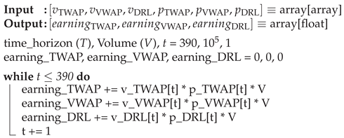
To eliminate this confusion, we also have calculated the monetary gain in $USD by the DRL models over TWAP and VWAP for the test market conditions. In Table 2, the results are depicted for AAPL (Large Cap), GDS (Mid Cap), ACMR (Small Cap) for the 3 market conditions. Here, the assumption is that the trader has 100,000 of each of the mentioned assets and the trader wants to liquidate them on a day randomly chosen from each of the 3 testing periods. The trader uses TWAP, VWAP and DRL method to liquidate each of the asset volumes.
The algorithm for the calculation of the monetary returns is explained in Algorithm 1.
As shown in the Table 2, DRL methods lets the trader earn much more than the model based methods. One interesting thing to note is that the monetary gain with DRL over VWAP is more than that with DRL over TWAP for AAPL on all the 3 testing days. It again confirms that for AAPL, TWAP outperforms VWAP. The Table 2 also confirms the failure of TWAP method for Mid and Small Caps in all of Normal and Stressful Market conditions.
| Algorithm 1: Calculation of monetary gain by DRL over TWAP/VWAP |
 |
4.2. Market Risks
One important aspect of this work is that unlike many other works, the market risk is taken under scrutiny. As mentioned earlier, even if the market is favorable for selling, the trader should not sell huge volume at a time in order to avoid market impacts. Different reasons behind market risks and different techniques to analyze them are explained in [15]. The reason why market impact is bad as it can lead to price slippage [7]. Price slippage is the sudden change in the price of the stock because of its buy or sell. When a buy order is placed, the price can increase due to higher demand, especially in limited supply conditions or when multiple players are also buying, while a sell order can cause the price to decrease, which intensifies with higher order volume.
To reduce the possibility of slippage, a penalty term in our reward function is introduced, as stated in equations (6) and (7). This is the second term of the reward equations. The principle of the penalty is that the quadratic power of it starts converging the total reward as the action starts to increase. It must be reminded that the action resembles the volume getting sold at time t.
There are different ways of visualizing the Risk involved. In this work, 3 approaches are taken. For all of the approaches, the assumption is that the trading agent sells 1% of total market sales. 3 instruments are chosen for 3 market situations:
1.AAPL (Large Cap) during Inflation+War (stressful market),
2.FLEX (Mid Cap) during Covid 1st spike (stressful market),
3.ENDP (Small Cap) during Normal Market Condition.
All of these results are in comparison to the VWAP method. And each of the studies are done for 20 trading days from the respective time period.
Figure 3 shows the most ’extreme minutes’ for the mentioned instruments, representing the minutes of the 390 trading minutes with the highest trade volumes on each of the 20 days. The ’extreme minute’ can be different for VWAP and DRL since VWAP often trades heavily at the first and last few hours of the day, while DRL does not follow this pattern. High trade volumes during the extreme minute can lead to significant Market Impacts, which is undesirable for both VWAP and DRL.
However, as shown in Figure 3a, the extreme trades by VWAP are very high with respect to that by DRL. For some days, the extreme trades by VWAP are about 50 to 100 times higher than the corresponding DRL trades. For Figure 3b, the extreme trades by VWAP are also very high with respect to the corresponding DRL trades. The performance by VWAP in Figure 3c is quite satisfactory except for a few days where the extreme trades by VWAP are again very high.
It is crucial to study the corresponding total market trades during the extreme minutes of VWAP and DRL methods, as there might be instances where DRL faces more market impacts than VWAP due to differences in their extreme trade timings and the corresponding total market trade volumes.
In Figure 4, the differences between the corresponding total market trades and the extreme trades made by VWAP or DRL are studied.
It is desired that this difference becomes significantly positive. This will mean that the trader is selling significantly less than the corresponding total market trades. However, for Figure 4a, it is seen that this difference for VWAP is a large negative. This means that VWAP ends up selling more than the corresponding total market trades. Fortunately, this difference for DRL is positive. The performances by both VWAP and DRL are positive in Figure 4b and Figure 4c.
In Figure 4, only the extreme minute for VWAP and DRL is considered, that is the minute of a day when each of them makes the maximum trade of the day. However, it would be worthwhile to study not only a single extreme minute but an average of some top extreme minutes of the day. In Figure 5, the top 10% of extreme minutes are studied. The differences between the corresponding total markets trades and trades by model for these top 10% of extreme minutes are calculated and at last an average out of these differences are measured.
In Figure 5a, it is seen that the difference values for AAPL using VWAP is still negative. For all of Figure 5a–c, we see a better performance by DRL than VWAP.
Lastly, the special case of FB (stock price of Meta) during the month of February 2022 is studied.
Because of the Inflation and War, FB price had been already declining. It started to plummet as its parent company Meta was sued because of privacy concern on 16th February, 2022. This is why, it is called a special case. As stated in Table 1, the performance of DRL for FB during Inflation and War is strikingly higher than that of VWAP (TWAP is benchmark model).
In Figure 6, the decreasing green dashed line represents FB’s price for the day. Both VWAP and DRL suggest trades well below the total market volume, indicating low market impacts. Both strategies trade only 1% of the total day’s volume, ensuring minimal market impact.
It can be seen that during the first few hours of the day when the price of FB was high, both the models suggest to trade more. However, during the rest of the hours of the first half of the day when the price was still relatively high, VWAP suggests to trade less. Because of its U-like shape, VWAP again asks to trade more at the ending few hours of the day, when the price of FB is the lowest. DRL, however, aligns perfectly with FB’s price, suggesting less selling as the price goes down and the least trade at the end of the day when FB’s price is lowest, resulting in a 0.1% performance improvement over VWAP with TWAP as the benchmark.
5. Conclusions and Discussion
In this study, robust Deep Reinforcement Learning (DRL) models were developed and compared to VWAP and TWAP in different market conditions for order execution. DRL consistently outperformed both models, achieving high returns and low risk even in stressful and volatile markets. With the strategies in section 1.2, the DRL models demonstrated a better understanding of the entire market, allowing them to outperform VWAP significantly. For example, PERI (Perion Network- a small Cap) received a bull market during Covid 2021. The price reached its all time high during this period. However, almost all of the assets’ prices in Russel 2000 were plummeting. Developing a model from only PERI’s data could turn out to be inefficient (performance improvement of VWAP over TWAP is only 0.0063%). The respective DRL model, which could grasp a much better portrait of the market, was significantly more efficient (performance improvement over TWAP is 0.38%).
While the DRL models consistently outperformed VWAP and TWAP in all test cases, the authors acknowledge that their superiority may not be guaranteed in every situation.
References
- Aurélien Alfonsi, Antje Fruth, and Alexander Schied. 2009. Optimal Execution Strategies in Limit Order Books with General Shape Functions. SSRN Electronic Journal (2009). [CrossRef]
- Robert Almgren and Neil Chriss. 2001. Optimal execution of portfolio transactions. The Journal of Risk 3, 2 (Jan. 2001), 5–39. [CrossRef]
- Bastien Baldacci and Jerome Benveniste. 2019. A Note on Almgren–Chriss Optimal Execution Problem with Geometric Brownian Motion. Market Microstructure and Liquidity 05, 01n04 (Dec. 2019). [CrossRef]
- Dimitris Bertsimas and Andrew Lo. 1998. Optimal Control of Execution Costs. Journal of Financial Markets 1, 1 (1998), 1–50. Available online: https://EconPapers.repec.org/RePEc:eee:finmar:v:1:y:1998:i:1:p:1-50.
- Sabri Boubaker, John W. Goodell, Dharen Kumar Pandey, and Vineeta Kumari. 2022. Heterogeneous impacts of wars on global equity markets: Evidence from the invasion of Ukraine. Finance Research Letters 48 (Aug. 2022), 102934. [CrossRef]
- Christine Brentani. 2004. Portfolio Management in Practice (Essential Capital Markets). Butterworth-Heinemann, Oxford, UK.
- Scott Brown, Timothy Koch, and Eric Powers. 2009. SLIPPAGE AND THE CHOICE OF MARKET OR LIMIT ORDERS IN FUTURES TRADING. Journal of Financial Research 32, 3 (Sept. 2009), 309–335. [CrossRef]
- Alvaro Cartea and Sebastian Jaimungal. 2015. Incorporating order-flow into optimal execution. Mathematics and Financial Economics 10 (2015), 339–364. [CrossRef]
- Alvaro Cartea, Sebastian Jaimungal, and Jose Penalva. 2015. Algorithmic and High-Frequency Trading. Cambridge University Press, Cambridge, UK.
- Arthur Charpentier, Romuald Elie, and Carl Remlinger. 2020. Reinforcement Learning in Economics and Finance. ArXiv abs/2003.10014 (2020).
- Jianyu Chen, Bodi Yuan, and Masayoshi Tomizuka. 2019. Model-free Deep Reinforcement Learning for Urban Autonomous Driving. In 2019 IEEE Intelligent Transportation Systems Conference (ITSC). IEEE. [CrossRef]
- Ming Deng, Markus Leippold, Alexander F. Wagner, and Qian Wang. 2022. Stock Prices and the Russia-Ukraine War: Sanctions, Energy and ESG. SSRN Electronic Journal (2022). [CrossRef]
- Joris Dinneweth, Abderrahmane Boubezoul, René Mandiau, and Stéphane Espié. 2022. Multi-agent reinforcement learning for autonomous vehicles: a survey. Autonomous Intelligent Systems 2, 1 (Nov. 2022). [CrossRef]
- Matthew Francis Dixon and Igor Halperin. 2020. G-Learner and GIRL: Goal Based Wealth Management with Reinforcement Learning. SSRN Electronic Journal (2020). [CrossRef]
- Kevin Dowd. 2007. Measuring Market Risk. John Wiley & Sons, NJ, USA.
- Yuchen Fang, Kan Ren, Weiqing Liu, Dong Zhou, Weinan Zhang, Jiang Bian, Yong Yu, and Tie-Yan Liu. 2021. Universal Trading for Order Execution with Oracle Policy Distillation. [CrossRef]
- Jonathan Federle and Victor Sehn. 2022. Costs of Proximity to War Zones: Stock Market Responses to the Russian Invasion of Ukraine. SSRN Electronic Journal (2022). [CrossRef]
- Shubha Ghosh and David M. Driesen. 2003. The Functions of Transaction Costs: Rethinking Transaction Cost Minimization in a World of Friction. SSRN Electronic Journal (2003). [CrossRef]
- John Greenwood and Steve H. Hanke. 2021. On Monetary Growth and Inflation in Leading Economies, 2021-2022: Relative Prices and the Overall Price Level. Journal of Applied Corporate Finance 33, 4 (Dec. 2021), 39–51. [CrossRef]
- Tobin Hanspal, Annika Weber, and Johannes Wohlfart. 2021. Exposure to the COVID-19 Stock Market Crash and Its Effect on Household Expectations. The Review of Economics and Statistics 103, 5 (Nov. 2021), 994–1010. [CrossRef]
- Jeff Heaton. 2017. Ian Goodfellow, Yoshua Bengio, and Aaron Courville: Deep learning. Genetic Programming and Evolvable Machines 19, 1-2 (Oct. 2017), 305–307. [CrossRef]
- Sepp Hochreiter and Jürgen Schmidhuber. 1997. Long Short-Term Memory. Neural Computation 9, 8 (Nov. 1997), 1735–1780. [CrossRef]
- L. P. Kaelbling, M. L. Littman, and A. W. Moore. 1996. Reinforcement Learning: A Survey. Journal of Artificial Intelligence Research 4 (May 1996), 237–285. [CrossRef]
- B Ravi Kiran, Ibrahim Sobh, Victor Talpaert, Patrick Mannion, Ahmad A. Al Sallab, Senthil Yogamani, and Patrick Perez. 2022. Deep Reinforcement Learning for Autonomous Driving: A Survey. IEEE Transactions on Intelligent Transportation Systems 23, 6 (June 2022), 4909–4926. [CrossRef]
- Yann LeCun, Yoshua Bengio, and Geoffrey Hinton. 2015. Deep learning. Nature 521, 7553 (May 2015), 436–444. [CrossRef]
- Yuxi Li. 2017. Deep Reinforcement Learning: An Overview. ArXiv abs/1701.07274 (2017). [CrossRef]
- Siyu Lin and Peter A. Beling. 2020. An End-to-End Optimal Trade Execution Framework based on Proximal Policy Optimization. In Proceedings of the Twenty-Ninth International Joint Conference on Artificial Intelligence. International Joint Conferences on Artificial Intelligence Organization. [CrossRef]
- Mieszko Mazur, Man Dang, and Miguel Vega. 2021. COVID-19 and the march 2020 stock market crash. Evidence from SnP500. Finance Research Letters 38 (Jan. 2021), 101690. [CrossRef]
- Volodymyr Mnih, Koray Kavukcuoglu, David Silver, Alex Graves, Ioannis Antonoglou, Daan Wierstra, and Martin Riedmiller. 2013. Playing Atari with Deep Reinforcement Learning. [CrossRef]
- Volodymyr Mnih, Koray Kavukcuoglu, David Silver, Andrei A. Rusu, Joel Veness, Marc G. Bellemare, Alex Graves, Martin Riedmiller, Andreas K. Fidjeland, Georg Ostrovski, Stig Petersen, Charles Beattie, Amir Sadik, Ioannis Antonoglou, Helen King, Dharshan Kumaran, Daan Wierstra, Shane Legg, and Demis Hassabis. 2015. Human-level control through deep reinforcement learning. Nature 518, 7540 (Feb. 2015), 529–533. [CrossRef]
- Yuriy Nevmyvaka, Yi Feng, and Michael Kearns. 2006. Reinforcement learning for optimized trade execution. In Proceedings of the 23rd international conference on Machine learning - ICML ’06. ACM Press. [CrossRef]
- Y. Nevmyvaka, M. Kearns, A. Papandreou, and K. Sycara. [n. d.]. Electronic Trading in Order-Driven Markets: Efficient Execution. In Seventh IEEE International Conference on E-Commerce Technology (CEC’05). IEEE. [CrossRef]
- Jürgen Schmidhuber. 2015. Deep learning in neural networks: An overview. Neural Networks 61 (Jan. 2015), 85–117. [CrossRef]
- Shai Shalev-Shwartz, Shaked Shammah, and Amnon Shashua. 2016. Safe, Multi-Agent, Reinforcement Learning for Autonomous Driving. ArXiv abs/1610.03295 (2016). [CrossRef]
- Min Shu, Ruiqiang Song, and Wei Zhu. 2021. The ‘COVID’ crash of the 2020 U.S. Stock market. The North American Journal of Economics and Finance 58 (Nov. 2021), 101497. [CrossRef]
- Philip Sommer and Stefano Pasquali. 2016. Liquidity-How to Capture a Multidimensional Beast. The Journal of Trading (March 2016). [CrossRef]
- Paul Stoewer, Christian Schlieker, Achim Schilling, Claus Metzner, Andreas Maier, and Patrick Krauss. 2022. Neural network based successor representations to form cognitive maps of space and language. Scientific Reports 12, 1 (July 2022). [CrossRef]
- R.S. Sutton and A.G. Barto. 1998. Reinforcement Learning: An Introduction. IEEE Transactions on Neural Networks 9, 5 (1998), 1054–1054. [CrossRef]
- Christopher J. C. H. Watkins and Peter Dayan. 1992. Q-learning. Machine Learning 8, 3-4 (May 1992), 279–292. [CrossRef]
- Kenta Yamada and Takayuki Mizuno. 2020. Analyses of Daily Market Impact Using Execution and Order Book Information. Frontiers in Physics 8 (Nov. 2020). [CrossRef]
- Deheng Ye, Guibin Chen, Wen Zhang, Sheng Chen, Bo Yuan, Bo Liu, Jia Chen, Zhao Liu, Fuhao Qiu, Hongsheng Yu, Yinyuting Yin, Bei Shi, Liang Wang, Tengfei Shi, Qiang Fu, Wei Yang, Lanxiao Huang, and Wei Liu. 2020. Towards Playing Full MOBA Games with Deep Reinforcement Learning. [CrossRef]
Figure 1.
Schematic Diagram of Deep Reinforcement Learning Model used in the present study.
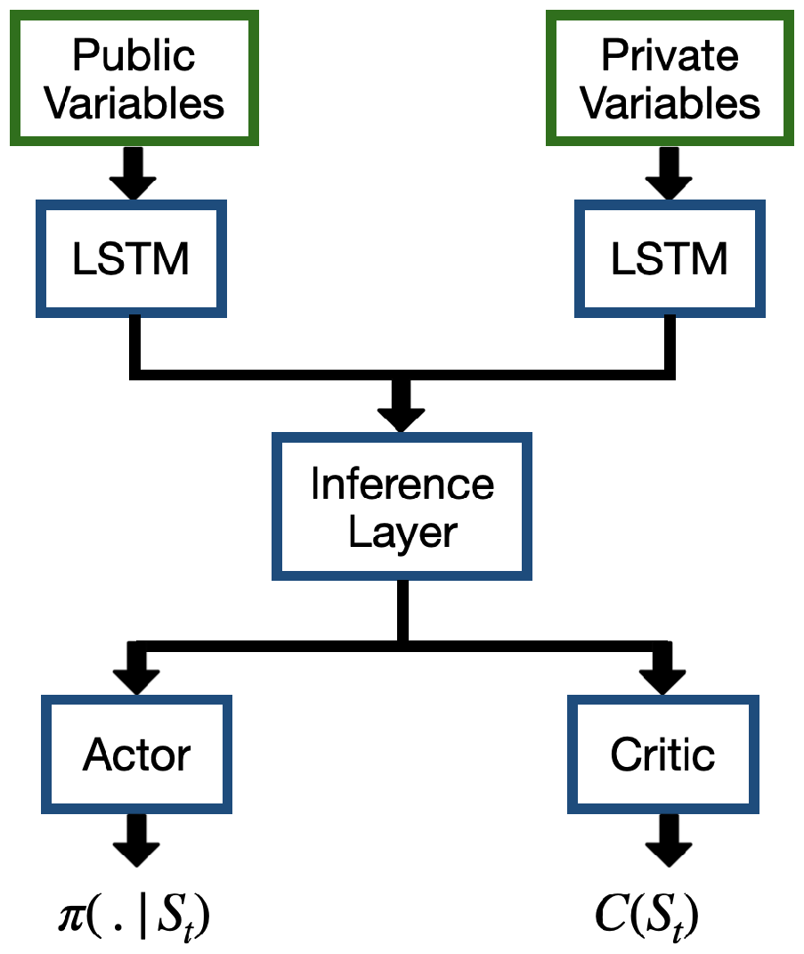
Figure 2.
(a) The Datasets of Large and Mid Caps are divided into 4 parts from April 2020 to mid March 2022. (b) The Datasets of Small Cap and ETFs are divided into 4 parts from April 2021 to mid March 2022.
Figure 2.
(a) The Datasets of Large and Mid Caps are divided into 4 parts from April 2020 to mid March 2022. (b) The Datasets of Small Cap and ETFs are divided into 4 parts from April 2021 to mid March 2022.
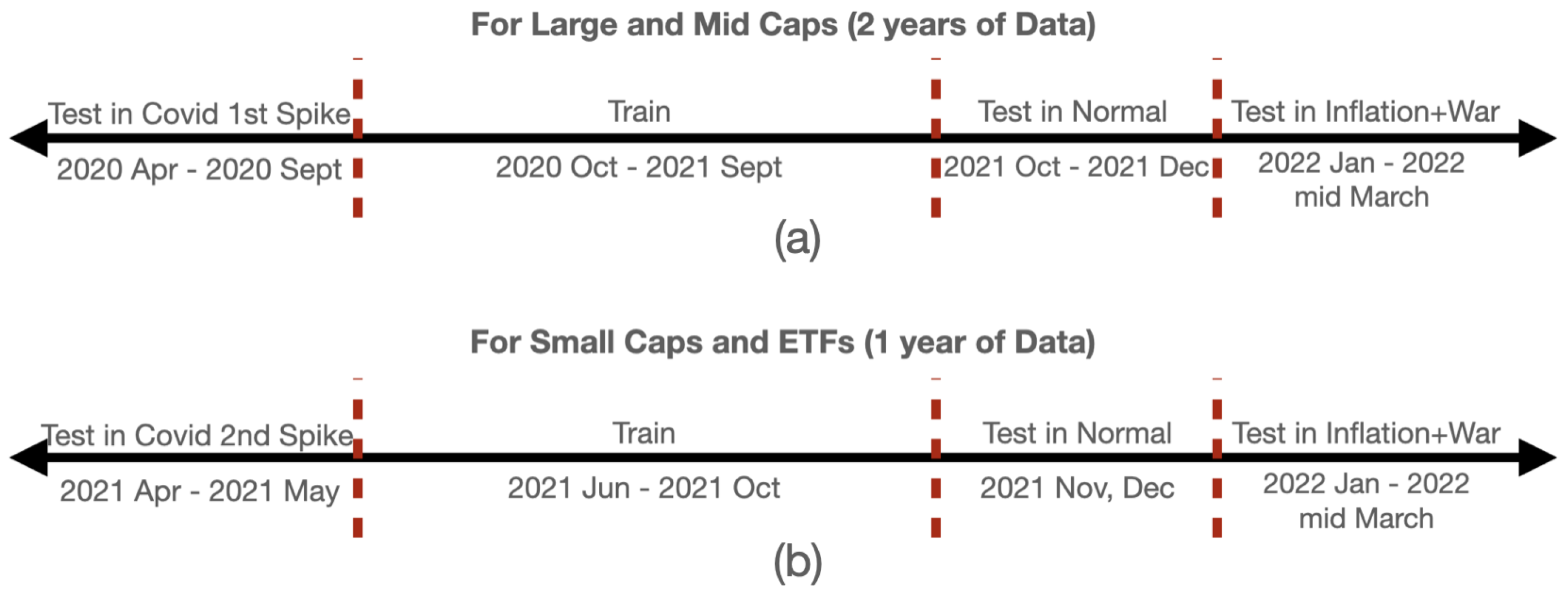
Figure 3.
Maximum Volume Sold at a Minute of all 390 Trading Minutes by VWAP and DRL for (a)AAPL during Inflation+War, (b)FLEX during Covid 1st spike, (c)ENDP during Normal Market
Figure 3.
Maximum Volume Sold at a Minute of all 390 Trading Minutes by VWAP and DRL for (a)AAPL during Inflation+War, (b)FLEX during Covid 1st spike, (c)ENDP during Normal Market
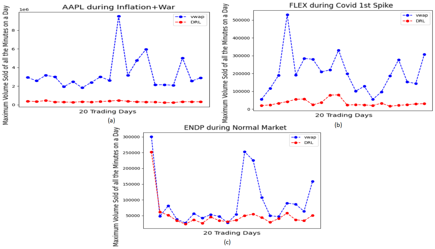
Figure 4.
(Total Market Trade - Trade made by model) at extreme minutes by VWAP and DRL for (a)AAPL during Inflation+War, (b)FLEX during Covid 1st spike, (c)ENDP during Normal Market
Figure 4.
(Total Market Trade - Trade made by model) at extreme minutes by VWAP and DRL for (a)AAPL during Inflation+War, (b)FLEX during Covid 1st spike, (c)ENDP during Normal Market
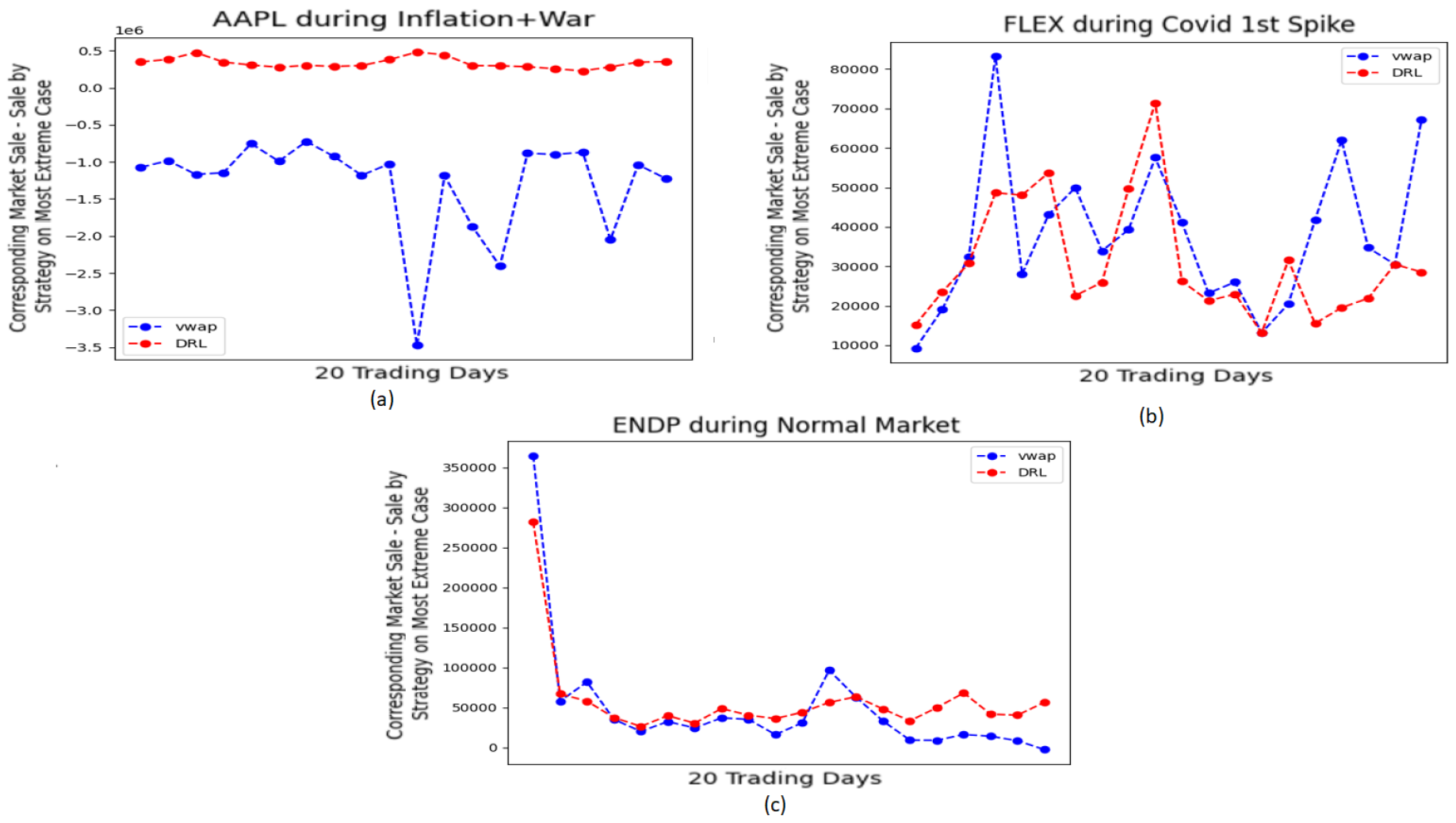
Figure 5.
Average of (Total Market Trade - Trade made by model) during top 10% extreme minutes by VWAP and DRL for (a)AAPL during Inflation+War, (b)FLEX during Covid 1st spike, (c)ENDP during Normal Market
Figure 5.
Average of (Total Market Trade - Trade made by model) during top 10% extreme minutes by VWAP and DRL for (a)AAPL during Inflation+War, (b)FLEX during Covid 1st spike, (c)ENDP during Normal Market
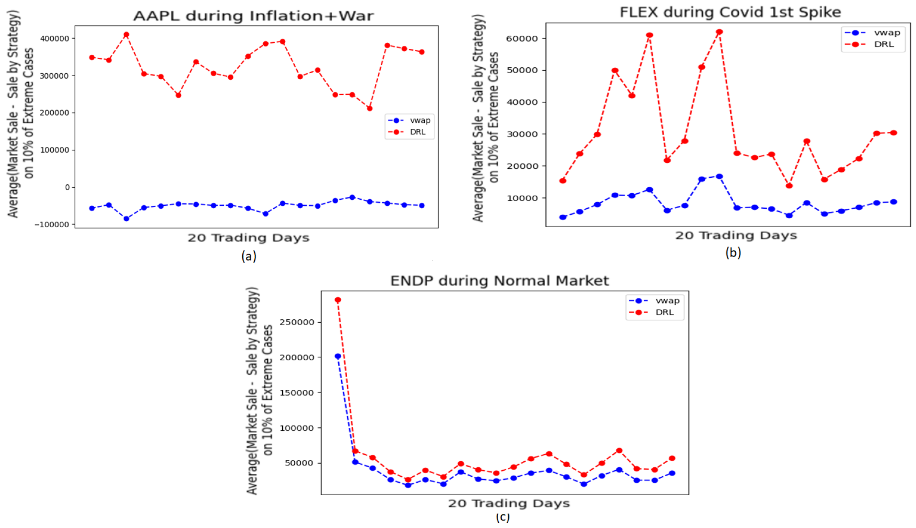
Figure 6.
FB on 16th February 2022 (not 100% in scale)
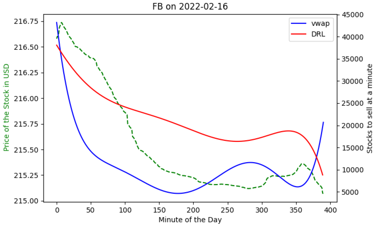

Table 1.
Performance improvements for VWAP and DRL keeping TWAP as benchmark.
| Stock | VWAP | DRL | VWAP | DRL | VWAP | DRL |
|---|---|---|---|---|---|---|
| Covid | Covid | Normal Market | Normal Market | Inflation+War | Inflation+War | |
| AAPL | -0.009 | 6.3161 | 1.59 | 2.68 | -0.027 | 0.59 |
| FB | -0.004 | 4.57 | -0.03 | 0.79 | -0.009 | 10.02 |
| IBM | 0.068 | 1 | 1.67 | 2.82 | 0.056 | 0.71 |
| MSFT | -0.009 | 2.434 | 1.61 | 2.44 | -0.015 | 0.77 |
| goog | 0.957 | 3.063 | 1.16 | 1.72 | 4.3 | 5 |
| AMZN | 0.104 | 5.175 | 2.5 | 3.05 | 0.48 | 1.1 |
| GDS | 5.65 | 11.56 | 17.9 | 18.58 | 9.68 | 10.46 |
| LECO | 45.125 | 47.3287 | 51.97 | 55.06 | 51.97 | 55.06 |
| FLEX | 1.18 | 4.18 | 5.6 | 6.2 | 1.66 | 2.53 |
| OLLI | 3.95 | 19.51 | 13.29 | 13.9 | 6.05 | 7 |
| SFIX | 1.44 | 11.01 | 3.5 | 10.9 | 0.32 | 7.63 |
| AMBA | 33.8 | 34.46 | 20.94 | 24.38 | 20.36 | 30.12 |
| ARES | 14.9 | 16.9 | 31 | 31.4 | 17.68 | 18.31 |
| VO | 8.8 | 10.2 | 12.5 | 13 | 5.18 | 5.72 |
| PRTS | 16.178 | 17 | 25.368 | 26.69 | 17.83 | 21.77 |
| PUBM | 23.09 | 29.56 | 11.8 | 20.63 | 9.1 | 12.74 |
| INSG | 5.168 | 7.06 | 9.48 | 11.62 | 11.43 | 13 |
| APPH | 7.48 | 13.64 | 10.55 | 12 | 27.73 | 28.86 |
| PERI | 0.63 | 37.603 | 34.2 | 36.5 | 27.73 | 29.03 |
| ARLO | 26.07 | 27.02 | 38.68 | 46.45 | 17.26 | 17.71 |
| ENDP | 3.31 | 9.74 | 6.14 | 8.1 | 2.82 | 7.53 |
| CVLT | 56.44 | 58.57 | 89.64 | 90.69 | 71.49 | 72.01 |
| NDAQ | 12.8 | 14.47 | 20.3 | 20.8 | 13.44 | 13.88 |
| DOW | 0.1 | 0.8 | 1.47 | 2.27 | 0.1 | 0.72 |
Table 2.
Improvements in Returns in $USD w.r.t. TWAP and VWAP by DRL.
| Stock | Covid | Normal Market | Inflation+War | |||
|---|---|---|---|---|---|---|
| TWAP | VWAP | TWAP | VWAP | TWAP | VWAP | |
| AAPL | $55,000 | $91,000 | $237,000 | $240,000 | $45,000 | $60,000 |
| GDS | $770,000 | $80,000 | $830,000 | $30,000 | $530,000 | $50,000 |
| ACMR | $4,830,000 | $40,000 | $6,100,000 | $40,000 | $4,170,000 | $50,000 |
Disclaimer/Publisher’s Note: The statements, opinions and data contained in all publications are solely those of the individual author(s) and contributor(s) and not of MDPI and/or the editor(s). MDPI and/or the editor(s) disclaim responsibility for any injury to people or property resulting from any ideas, methods, instructions or products referred to in the content. |
© 2025 by the authors. Licensee MDPI, Basel, Switzerland. This article is an open access article distributed under the terms and conditions of the Creative Commons Attribution (CC BY) license (http://creativecommons.org/licenses/by/4.0/).
Copyright: This open access article is published under a Creative Commons CC BY 4.0 license, which permit the free download, distribution, and reuse, provided that the author and preprint are cited in any reuse.


