Submitted:
17 November 2025
Posted:
19 November 2025
You are already at the latest version
Abstract
This work establishes a large language model (LLM) specialized in the domain of thermoelectric generators (TEGs), for deployment on local hardware. Starting with the generalist JanV1-4B model, an efficient fine-tuning (FT) methodology (QLoRA) was employed, modifying only 3.18% of the total parameters of this base model. The key to the process is the use of a custom-designed dataset, which merges deep theoretical knowledge with rigorous instruction tuning to refine behavior and mitigate catastrophic forgetting. Performance evaluation, conducted using a questionnaire of increasing complexity, revealed that the FT JanV1-4B-expert-TEG modelled in this work achieves an overall accuracy of 81%, demonstrating capabilities ranging from the correct formulation of equations to critical design reasoning. This study validates the specialization of LLMs using QLoRA as an effective and accessible strategy for developing highly competent engineering support tools, eliminating dependence on large-scale computing infrastructures.
Keywords:
LLM
; QLoRA
; JanV1-4B
; fine-tuning
; thermoelectric generators
1. Introduction
Recent advances in large language models (LLMs) have opened new frontiers for assisting with complex engineering design tasks [1]. However, their effective application in highly specialized domains faces two main challenges: the lack of deep, domain-specific knowledge, which limits their accuracy and reliability, and the high computational and energy costs associated with their training and deployment.
This work addresses this gap by proposing a practical and accessible solution: the creation of a domain-specific, specialist AI assistant designed to operate efficiently on local hardware. The domain chosen to validate this hypothesis is thermoelectric generators (TEGs), a field that perfectly encapsulates engineering complexity. Their modeling requires a deep understanding of coupled physical phenomena such as the Seebeck, Peltier, and Joule effects, the formulation of nonlinear differential equation systems, and critical reasoning for design optimization. The goal, therefore, is to develop a tool that can reason, model, and analyze like a specialist engineer, thereby overcoming the limitations of generalist LLMs that often fall short of the required accuracy and technical depth, and going beyond the simple creation of a repository of information.
This study focuses on the domain of TEGs, solid-state devices that convert thermal energy directly into direct current electricity using the Seebeck and Peltier effects [2]. Due to the absence of moving parts, they operate silently, making them ideal for applications in remote locations where thermal energy is the primary available source. However, their modeling and optimization are considerably complex. The performance of TEGs is intrinsically linked to the interrelation of coupled thermal and electrical phenomena, often described by systems of nonlinear partial differential equations [3]. Furthermore, factors such as the geometric configuration decisively influence their maximum power output [4]. To address this domain, this article uses a four-degree-of-freedom lumped-parameter model [5], on which the variants used for LLM training are generated.
This work addresses the gap between the potential of LLMs and the demands of this specialized TEG domain, presenting a methodology for developing a specialist LLM based on the four-billion-parameter (4B) JanV1-4B generalist base model [6], designed for application in local environments. It is called a base model because it has not yet been refined.
To overcome computational limitations and facilitate its use on consumer hardware, parameter-efficient fine-tuning (PEFT) techniques are employed [7,8]. These methods have demonstrated performance comparable to full fine-tuning (FT) by training only a minimal fraction of the parameters (<1%). In particular, this work implements the quantized low-rank adaptation (QLoRA) technique [9], an evolution of LoRA [10] that maximizes memory efficiency and makes FT accessible on consumer hardware. This approach not only validates the creation of an expert model in a highly complex field but also demonstrates the feasibility of democratizing access to advanced AI tools by eliminating dependence on large-scale computing infrastructures.
The core of our methodology is based on two fundamental pillars.
First, the development of a custom-designed training dataset that combines deep domain knowledge —including physical principles, fundamental equations, and terminology— with a training dataset of instructions. This latter component is crucial for refining the model's behavior, ensuring it follows complex guidelines, and, fundamentally, mitigating catastrophic forgetting [11] of its general knowledge. The primacy of quality over quantity in the training dataset is a guiding principle in this work and a thesis empirically demonstrated in foundational studies such as LIMA (Less Is More for Alignment) [12], which validate the use of small but high-quality datasets to achieve exceptional performance.
Second, the implementation of a rigorous multilevel assessment framework. This framework is designed to measure a spectrum of cognitive abilities, from retrieving fundamental knowledge and applying mathematical models to qualitative design reasoning and critical analysis of numerical data. This article not only presents the development of the specialist LLMs but also provides a comprehensive validation of their performance, detailing their strengths and areas for improvement. The network was trained on a well-curated dataset of concepts obtained from references in the TEG field [13,14,15,16,17].
The fundamental contributions of this work are four.
First, a comprehensive and reproducible methodology is presented, from data curation to local deployment, to transform a general purpose LLM JanV1-4B [6] into a specialist assistant within a highly specialized engineering domain in TEG.
Second, a strategic design is proposed for a training dataset that balances the injection of deep knowledge —the "what"— with the shaping of behavior and response ability —the "how"— which is key to mitigating catastrophic forgetting and achieving robust performance.
Third, a rigorous multi-level assessment framework is introduced that measures advanced cognitive abilities, such as critical reasoning and self-correction, going beyond traditional metrics.
And fourth, it is empirically demonstrated that it is feasible to achieve this high level of specialization using local hardware, validating the QLoRA approach as an effective way to democratize the development of specialist AI in TEG.
This document is structured as follows: Section 2 presents the lumped-parameter mathematical model of the TEG, which serves as the knowledge base and reference for the evaluation. Section 3 explains the FT methodology. Section 4 describes the composition of the FT dataset. Section 5 presents and discusses the results obtained. Finally, Section 6 offers the main conclusions regarding the LLMs specializing in the field of TEG engineering that have been developed in this work.
2. Mathematical Model of the TEG
This section details the lumped-parameter mathematical model that describes the behavior of a TEG. This model fulfills two fundamental functions in this work: first, it serves as the basis for the synthetic generation of the dataset used in the FT LLM; and second, it constitutes the reference or ground truth for the quantitative validation of the responses generated by the expert model to questions related to its equations.
The operating principle of a TEG is based on the application of heat flow from a high-temperature source, , to a lower-temperature sink, . This flow induces a temperature difference between the hot and cold faces of the device, which, due to the Seebeck effect, generates a direct current voltage. The objective of the model is, therefore, to establish a system of equations that allows calculation of the temperatures on the module's faces in order to determine key performance metrics, such as the electrical power supplied to an external load.
2.1. Definition of Parameters and Variables
Figure 1 presents a simplified scheme of a TEG, showing its essential elements: heat source, heat sink, n-type and p-type semiconductors, structural heat-conducting ceramics, and the electric charge .
To construct this system, a thermoelectric analogy is used, whose equivalent circuit is illustrated in the thermal circuit shown in Figure 2. Under this analogy: the heat flow [W] is modeled as if it were an electric current, and the temperature [K] is represented as if it were an electric potential, taking absolute zero as the ground reference node.
2.2. Transient Regime Analysis
The circuit shown in Figure 2 is a proper nonlinear circuit. Its complexity order is four. The four state variables are represented in the following vector,
The input vector is composed of the external temperature sources expressed by the following equation:
The equations are presented as the energy balance at the four nodes of the thermal circuit in Figure 2 shown in the following equation:
The voltage used to calculate the current of the electrical circuit is expressed according to the following equation:
The balance at node , inner hot face, including the energy accumulation term, is given by the following equation:
By solving for the derivative and substituting , we obtain the first equation of state:
Similarly, the balance at node , internal cold face, is:
By solving for the derivative of equation 7 and substituting expressed in equation 4, we obtain the second equation of state:
The balance at node , external hot ceramic, depends on the inlet heat source , as can be seen in the following equation:
By solving for the derivative, we obtain the third equation of state:
The balance at node , external cold ceramic, depends on the ambient temperature , as can be seen in the following equation:
And finally, by solving for the derivative, we obtain the fourth equation of state:
The complete system of nonlinear differential equations of the transient thermal and electrical circuit that describe the dynamics of the TEG is expressed by equations 13 to 16:
This system has the form and is ready to be solved numerically using an ordinary differential equation integrator (ODE) [18], to simulate the transient behavior of the system under changes in or .
2.3. Stationary Regime Analysis
The steady-state analysis will be studied in two steps: the establishment of the balance equations, and the development of the Jacobian and the second member of the system of equations.
2.3.1. Energy Balance Equations
In steady state, the partial derivatives with respect to time are zero, so equations 13 to 16 simplify considerably. It should be noted that in this case the resulting equations remain nonlinear.
To solve this nonlinear system using the Newton-Raphson method, the linear system to be solved in each iteration is set up as shown in the following equation:
where is:
To obtain greater numerical robustness, by searching for the diagonal domain, the system of equations is defined by equations 19 to 22.
- Function 1, balance at :
- Function 2, balance at :
- Function 3, balance at :
- Function 4, balance at :
2.3.2. Solving Nonlinear Equations
To solve the system of nonlinear equations in steady state using the Newton-Raphson method, it is necessary to calculate the Jacobian matrix and the second member vector of equation 17. The state vector is .
The functions of the system are expressed by equations 19 to 22.
The Jacobian matrix is defined as the matrix of first-order partial derivatives, where takes the form:
The elements of the matrix are given by equations 24 to 39:
The Newton-Raphson iterative system is which is expressed by equation 17.
The vector of the second member is calculated as:
The terms and are as follows:
And the terms and take the following form
for , the calculation of results in:
and likewise, for we obtain:
Grouping all the components, we obtain the following expression which gives us the second member of the system of equations in steady state:
3. FT Methodology
The FT process was run on a Linux platform with an NVIDIA GeForce RTX 2070 SUPER GPU. To optimize memory usage and accelerate training, the open-source Unsloth library [19] was used, applying its optimizations to the base model JanV1-4B [6]. According to its developers, this model is an FT of Qwen3-4B-Thinking, an architecture belonging to the Qwen2 model family [20]. Training on 202 questions and answers (QA) found in this work's repository [21] over three epochs was highly efficient, completing in just 263 s. Each data sample was structured using a chat template that included a powerful system prompt, training the model to behave like an expert in thermoelectric materials and to proactively clarify ambiguous concepts, such as the definition of the power coefficient.
Monitoring training loss across the three epochs confirmed the effectiveness of the FT methodology. Starting with an initial loss of 2.38, the model showed the greatest learning gain during the second epoch, where the loss decreased by 13.6%. This process continued steadily, with an additional 7.4% reduction in the third epoch, culminating in a final loss value of 1.91. This reduction represents a total decrease of 19.9% and indicates robust and progressive learning. Furthermore, the gradient norm remained controlled throughout the process, confirming the stability of the convergence and the suitability of the selected hyperparameters. This indicates that the model successfully assimilated the new data.
Using the LoRA technique, 132,120,576 parameters were tuned, representing only 3.18% of the total architecture (4.15×10⁹ parameters). The model was loaded in a 4-bit format to drastically minimize its memory footprint. A maximum context window of 2048 tokens was configured, striking a balance between the ability to process complex information and computational limitations. A conservative learning rate of 2×10⁻⁶ was applied, with a linear decline throughout training, to gradually integrate new knowledge without compromising the model's existing capabilities.
The workflow concluded with the merging of the adapters and subsequent conversion to the Georgi Gerganov Universal Format (GGUF) [22], leaving it ready for efficient inference in local environments.
The following diagram illustrates the complete cycle for specializing a JanV1-4B general-purpose LLM into a TEG domain expert, using an efficient and reproducible workflow. This new model is called the JanV1-4B-expert-TEG model. The process begins with the base JanV1-4B model and culminates in its specialization in the field of thermoelectricity, TEG. It is divided into four key phases, summarized in Figure 3.
Phase 1: Preparation & FT (the TEG specialist's workshop).
The starting point consists of two essential components: a pre-trained JanV1-4B base model and a curated expert dataset with domain-specific knowledge —in this case, 202 QA on TEG [21].
Instead of retraining the entire model, which is computationally prohibitive, we applied the QLoRA technique. A Python script called train.py [21] was written, which freezes the base 4B model and trains only a small set of new weights, called the LoRA adapter. This adapter, representing only a tiny fraction of the total model size (3.18%), learns the new skills and knowledge of the dataset. The result of this phase is not a new model, but rather this lightweight and portable adapter.
Phase 2: Consolidation & Optimization.
Once we have created a new adapter, we need to integrate it to create a standalone efficient model. This process has two steps:
- Merging: A script, merge.py [21], was created to combine the weights of the original JanV1-4B base model with those of the LoRA adapter. The result is a complete merged expert model in the Hugging Face standard format [23]. This yields a single model containing both the general knowledge and the new specialization.
- GGUF Conversion & Quantization: To make the model practical and fast for inference in real-world use, we converted it to GGUF format using the tools from the open-source project llama.cpp [22]. During this step, 4-bit quantization was also applied, a process that drastically reduces file size and RAM usage with minimal loss of precision. The result is a single file with the .gguf extension, optimized for efficient execution on both CPUs and GPUs.
Phase 3: Deployment & Serving (Go-Live).
With the optimized model in GGUF format, the next step is to make it accessible. For deploying and running the LLM model in a local environment, the open-source framework Ollama [24] was used, which simplifies LLM management and inference on consumer hardware. Using a file called a modelfile [21], which acts as a configuration recipe, we tell Ollama where to find the GGUF file and how the model should behave, for example by providing its system prompt.
The ollama create command packages the result of this phase and registers the model on the local system. From this point on, the expert model is deployed and ready to be invoked with a simple command called ollama run and the expert model name, JanV1-expert-TEG.
Phase 4: Usage & Evaluation (Advanced quality control).
Next, it is crucial to verify the performance of the new JanV1-expert-TEG model through a qualitative and an advanced evaluation.
- Qualitative evaluation: This involves interacting directly with the model, just as a human expert would. We ask complex questions and evaluate the coherence, technical accuracy, and style of its responses. It is a subjective but fundamental test.
- Advanced evaluation: To ensure the highest quality of the expert model, a rigorous dual evaluation process is implemented that surpasses traditional metrics. First, a qualitative evaluation is performed, where human subject matter experts review the model's responses to validate their technical accuracy, consistency, and practical utility in real-world scenarios. Next, a cutting-edge technique known as LLM-as-a-Judge [25,26] is applied. In this step, state-of-the-art language models GPT-4 [25] and Gemini 1.5 Pro [26] are used to act as impartial evaluators, scoring the expert model's responses based on their quality, relevance, and correctness. This combined approach provides a much deeper and more nuanced assessment than traditional automated metrics [27], as it is able to analyze the reasoning and semantic quality of the responses, not just word matching.
If, at the end of phase 4 in Figure 3, the analysis result is not acceptable, the dataset can be expanded by returning to phase 1. In this way, the results of this evaluation phase feed into a continuous improvement cycle, providing input on how to refine the dataset or how to adjust the hyperparameters for the next FT iteration, if necessary. In our case, the dataset was improved with 12 iterations.
This methodology for obtaining the FT explained for the LLM JanV1-4B-expert-TEG represented in the diagram of Figure 3 was also applied in the LLM Qwen3-4B-thinking-2507-TEG.
These two LLMs were refined because they had the best scores in the published generalist benchmarks, as will be justified later in section 5.2 TEG FT models vs. generalist LLMs.
4. Dataset Definition
To construct the training dataset for the FT LLM, information on the progress and applications of TEG [28] was used, among other things. Concepts and laws related to TEG were classified, and reviews of the current state of TEG were taken into account [2,13,29]. Additionally, a QA dataset related to the model developed in section 2 was created.
To explain the criteria for choosing the content of the dataset, a flowchart has been made, see Figure 4, which is explained below.
This diagram visualizes the composition of the dataset used for the model's technical testing and allows for the classification of QA elements categorized into subsets. The objective of this dataset is not only to teach the model new information but also to shape its behavior. The diagram shows a strategic division into two main branches: knowledge injection and behavior shaping.
Within the knowledge injection branch, there is a subset called Domain-Specific data that comprises 48.5% of the dataset. Its purpose is to make the model an expert in a specific field, in this case, thermoelectricity. It is subdivided into:
a) Pure Domain (46.0%): The largest portion of the dataset focuses on pure factual knowledge, theoretical concepts, and terminology. This is the knowledge from scientific articles.
b) Calculation (2.5%): A small but critical part dedicated to teaching the model how to apply mathematical formulas from the domain to solve practical problems.
Within the behavior shaping branch, there is a subset called Instruction-Tuning data that comprises 51.5% of the dataset. This data is not about teaching what to say, but how to say it. It shapes the model's behavior, response style, and safety. It is divided into:
a) Skill-based (47.5%): A very significant portion, now the largest in the dataset, is dedicated to teaching the model how to structure complex responses —such as those involving equations— consistently and clearly, regardless of the specific instruction. This improves the quality and usability of the model's responses.
b) General Purpose (4.0%): This acts as a safeguard against catastrophic forgetting and overspecialization. It includes general knowledge and safety guidelines to ensure the model remains versatile and does not lose its core competencies after being tailored to such a specific topic.
Logically, some categories can be fuzzy, belonging to different subsets depending on the case. This is a common challenge in data classification. Although the diagram in Figure 4 uses a closed classification implying a single main category, the reality is often more complex.
For example, a classified dataset entry referenced as applied numerical calculations could also have been referenced as a response skill such as presenting the calculation and the result.
To represent this overlap in the flowchart, a non-directional dashed line has been added between the Calculation and Skill-based nodes. This visually indicates a strong conceptual link and potential overlap between these two subsets, even though they are formally separated in the dataset classification.
The composition and strategy of the 202 QA dataset used in the FT process are detailed in Table 2. This dataset was meticulously designed to address not only the "what" —knowledge— but also the "how" —responsiveness— a crucial aspect for developing an expert and reliable LLM.
The generation of the dataset is based on two fundamental pillars that coincide with the branches mentioned above: knowledge injection of the TEG domain and behavior shaping of the dataset.
Pillar 1: Knowledge injection of the TEG domain.
This pillar introduces 93 QA, representing 48.5% of the total QA. The main objective of this section is to build a solid and comprehensive knowledge base in the field of thermoelectricity.
This pillar forms the theoretical basis of the model. It covers fundamental definitions such as the Seebeck effect and the merit factor ZT [30], properties of key materials used in TEGs (PbTe, SnSe, skutterudites) [31,32,33], various applications (sensors, automotive, radioisotope thermoelectric generators, etc.), and essential physical principles such as the Wiedemann-Frenz Law [34]. The extensive QA in this section ensures that the model possesses the vocabulary and conceptual framework of an expert.
The applied calculations are presented through 5 QA. Although numerically small, this subset is functionally critical. It teaches the model to perform direct calculations, such as determining thermal conductance or internal resistance from geometric and material parameters, validating its ability to apply formulas.
Pillar 2: Behavior shaping of the dataset.
This pillar introduces 104 QA, representing 51.5% of the total QA. This pillar, the largest in the dataset, focuses on teaching the model to act like an engineer, structuring responses, formulating models, and recognizing the limits of its knowledge.
The skills and format are developed through 96 QAs. This is the core of the Instruction-Tuning data. The four-degree-of-freedom lumped-parameter mathematical models developed in section 2 are included, along with dozens of variations from the Instruction-Tuning data —formulate, derive, analyze, give me the equations, translate this netlist, etc. This repetition with variation technique is fundamental for the model to learn to recognize the underlying intent of a question, regardless of how it is phrased, and to always respond with a consistent and well-formatted structure —bold headings, lists, LaTeX formatting for equations, etc. It is direct training for robustness and reliability.
General knowledge and safety are addressed through 8 QA. These inputs act as safety railings or regulators. Including general knowledge questions —such as who painted the Mona Lisa?— helps mitigate catastrophic forgetting, preventing the model from overspecializing to the point of losing its general capabilities. Safety examples are also included to teach the model to identify and reject domain-insensitive questions —such as calculate the efficiency of a potato— which is an essential skill for a reliable AI assistant.
Of these 104 QA, 20 were established to clarify ambiguous concepts, specifically differentiating the thermoelectric power coefficient —a concept specific to thermoelectric generators— from the power factor of alternating current circuits —a general electrical concept. This deliberate repetition of the same question posed in different ways inscribes a conceptual distinction in the LLM that is often confusing, teaching the model to be precise and to actively correct common misunderstandings.
Furthermore, continuous expansion and improvement are implemented, as the dataset is designed to be a living resource that can be extended. Areas such as numerical calculations and complex design reasoning can be easily expanded. For example, by adding problems that require the model to deduce properties from experimental results or to propose TEG designs for specific scenarios. For instance, the specialized LLM could be tasked with designing a TEG for an industrial furnace at 800 K, justifying the choice of materials.
In conclusion, this dataset of 202 QA is a robust and strategically balanced dataset. Its dual approach, combining a deep knowledge base with rigorous training in response format and structure, is key to achieving an expert model not only in terminology but also in the mathematical modeling of the TEGs.
5. Results and Discussion
This section examines the inference of the two refined models developed in this work: JanV1-4B-expert-TEG and Qwen3-4B-thinking-2507-TEG. It also includes a comparative analysis of these two models against five other unrefined baseline models.
5.1. Analysis by Level of Difficulty
To validate the capabilities of the LLM JanV1-4B-expert-TEG that was trained with a dataset of 202 QA (see Figure 3), a structured questionnaire of 16 questions [21] was designed, which is shown in Table 3. The performance of the LLM was evaluated as excellent, correct with difficulties, and incorrect.
To perform this inference, the trained model must be deployed in the Ollama environment [24]. This is done by executing the command ollama run JanV1-4B-expert-TEG. As a result of this execution, the Python command prompt appears, where questions are asked and the corresponding answers are obtained.
The 16 questions were classified into four levels of difficulty and cognitive domain to allow for granular analysis of the model's performance:
- Level 1: Formulation. Questions that require the direct formulation of heat balance equations for a single node. Questions 1, 2, 8, 9 and 11.
- Level 2: Application of models. Questions that involve combining multiple heat flows, handling thermoelectric interactions, or simplifying equations under new conditions. Questions 3 to 7.
- Level 3: Qualitative & Design reasoning. Questions that require a conceptual analysis of design trade-offs, without complex numerical calculations. Questions 10 and 12.
- Level 4-5: Quantitative & Critical analysis. Questions that require numerical calculations, interpretation of tabulated data, and decision-making based on multidimensional analysis. Questions 13 to 16.
5.1.1. Level 1: Formulation
LLM JanV1-4B-expert-TEG answered all questions at this level flawlessly and without hesitation. It demonstrated a solid understanding of heat balance principles and was able to formulate the differential equations correctly. For example, for question 2 [21] concerning the heat power balance of the dissipation node , it generated the following answer, which is correct:
5.1.2. Level 2: Application of Models
Performance at this level was mostly excellent. The model correctly handled the inclusion of Joule and Peltier thermoelectric effects, and the simplification of equations in specific scenarios —open electrical circuit, .
The only difficulty arose in question 5, which requested the complete system of equations for all four nodes. The model initially struggled to structure the response, although the final equation for the most complex node, , was correct.
For question 4, it correctly provided the two internal equations. For example, for the hot junction equation , the following correct expression was obtained:
5.1.3. Level 3: Qualitative & Design Reasoning
In this category, LLM JanV1-4B-expert-TEG demonstrated a remarkable capacity for abstract reasoning. In question 12, regarding the geometry of the TEG's legs, the model was able to self-correct and arrived at the correct conclusion about the fundamental trade-off between electrical resistance and thermal conductance. This indicates second-order reasoning, where the LLM not only applies formulas but also understands the underlying design principles.
5.1.4. Level 4 and 5: Quantitative & Critical Analysis
This level of assessment was designed to measure the model's more advanced cognitive abilities: quantitative analysis of numerical data, critical reasoning, and engineering decision-making. To this end, a numerical experiment was designed focusing on question 16, which simulated a scenario involving the analysis of optimization results for the parameters of the equivalent circuit in steady state.
The objective of the simulation was to identify the optimal parameters of the TEG model by comparing four different optimization methods: the canonical genetic algorithm (GA) [35], a variant of GA with niche formation for real spaces (niching) that seeks to explore multiple local optima (NGA) [36], the differential evolution (DE) algorithm [37], and, finally, the simplicial homology global optimization (SHGO) method [38], available in the SciPy 1.15.2 library [18].
LLM JanV1-4B-expert-TEG was provided with the results of this process in the form of Table 4 and Table 5 and assigned the role of a TEG expert data analyst. Their task was to analyze the final error, simulation accuracy, and runtime of each algorithm to ultimately determine the best option and justify their choice based on a practical trade-off. The performance results and parameters identified for each algorithm are summarized in Table 4. Table 5 presents a comparison of the runtime, final objective function error, and optimal parameter values found by each of the four methods.
Based on the reference data used for the TEG Peltier cell model ET-031-10-20 [5], the final steady-state model of equation 17 was solved.
The summarized results are as follows:
- Actual target values: , , ,
, , y .
To validate the accuracy of the identified parameters, the temperatures simulated by each optimized model were compared with the reference values obtained in the simulation. Table 5 presents this comparison for the two extreme operating points of the studied range, 0.0 and 90.0 °C, corresponding to the minimum and maximum temperatures of the heat source, . In other words, a comparison is presented between the experimental and simulated temperatures using the parameters obtained with the four optimization algorithms at points and , at the extremes of the operating range.
The LLM demonstrated exceptional competence in this task. Not only did it correctly and unequivocally identify the worst-performing algorithm, SHGO, but it also addressed the apparent conflict between the metrics in the two tables. It considered that, although one algorithm had a theoretically lower final error, the DE algorithm showed excellent practical accuracy in simulating real-world temperatures. It pragmatically and with good justification concluded that DE was the better option, due to its excellent balance between high accuracy and significantly higher speed.
This result is particularly relevant, as it demonstrates that the specialized LLM is not limited to retrieving information, but is capable of performing synthesis and critical analysis equivalent to that of a human expert in a realistic engineering scenario.
Therefore, small LLMs can reason, since although this model only has 4B, it demonstrated an ability for logical reasoning, comparison and synthesis when given the appropriate framework to work in.
In other questions at this level, the performance was outstanding. The LLM handled unit conversions, ZT figure of merit calculations, and temperature-dependent property analyses with ease.
The model occasionally showed initial difficulties when faced with questions requiring the synthesis of a complete system of equations, such as question 5 of the questionnaire [21], which requested the complete system of equations for all four nodes. However, parts of the problem were eventually solved correctly. This suggests that structuring prompts for highly complex problems remains crucial.
Table 3 summarizes the 16 questions of the TEG expert questionnaire and the evaluation level achieved in the inference of the LLM trained with FT. The evaluation process is summarized in the flowchart in Figure 5. The overall accuracy analysis is 94%. In this way, the LLM JanV1-4B-expert-TEG showed high performance and domain-specific reasoning.
5.2. TEG FT Models vs. Generalist LLMs
This section aims to compare the specialized FT models developed in this work —JanV1-4B-expert-TEG and Qwen3-4B-thinking-2507-TEG— with other generalist models between 4B and 8B. More specifically, the Mistral-7B [39], Llama3-8B [40], Qwen3-4B-thinking-2507 [41], Qwen2-7B [42], and Janv1-4B [6] models are compared against a set of 42 specialized thermoelectricity questions developed in this work called the Specialized Thermoelectricity Benchmark [21].
The analysis of the inference of the previous models on 42 questions about TEG is shown in Figure 6. The clear superiority of the JanV1-expert-TEG model (81%) compared to its base version, Janv1-4B (31%), from which it is derived, is evident. The refinement was not an incremental improvement, but rather a qualitative leap that transformed a base model with low capacity for this domain in TEG into a highly competent and reliable one. This demonstrates that, for specialized domains, technical sensing is the most effective strategy for achieving expert performance.
The Qwen3-4B-Thinking-2507 model (76.2%) is the most interesting case. Despite being a base model without specific tuning, its performance is exceptionally high, almost on a par with the FT JanV1-4B-expert-TEG model. This suggests that it possesses a pre-existing architecture and training with a logical and mathematical reasoning capacity far superior to the average, allowing it to learn and correctly apply the formulas it deduces from the context.
This is consistent when comparing the performance of this model in five very demanding benchmarks. GPQA [43], with graduate-level science questions requiring deep reasoning, AIME25 [44], with a well-known, highly challenging mathematics exam, LiveCodeBench v6 [45], consisting of a code generation and problem-solving test, Arena-Hard v2 [46], which is based on a set of challenging questions where the quality of the model's response is assessed, and finally BFCL-v3 [47], another benchmark designed to assess logical reasoning and comprehension. Table 6 compares the metrics of the five benchmarks [41].
In contrast, the standard base models JanV1-4B (30.9%) and Qwen2-7B (23.8%) represent the typical performance of a base model (see Figure 6). They have some conceptual knowledge —they know what the Peltier effect is or what a semiconductor is doped for— but they fail in applying the formulas.
The most popular generalist models, such as Mistral-7B (7.1%) and Llama3-8B (4.8%), perform very poorly. This result is critical because it demonstrates that a larger model size, 7B and 8B in this case, does not guarantee greater competence in a specialized technical domain like TEG. Lacking specific knowledge, these models appeal to hallucination [48], inventing formulas and concepts, which makes them not only useless but dangerously misleading for this task.
Figure 6 perfectly illustrates three levels of competence: the specialized level —achieved with FT in the two models refined in this work, JanV1-4B-expert-TEG and Qwen3-4B-Thinking-2507-TEG— the high-potential level — Qwen3-4B-Thinking-2507, generalist model with strong reasoning— and the incompetence level —generalist models that are simply unrealistic, JanV1-4B, Quen2-7B, Mistral-7B and Llama3-8B. This is very powerful quantitative evidence of the value of specific benchmarks and the impact of FT.
The analysis of the results reveals the following:
- 1.
- General knowledge is insufficient, as very powerful general-purpose models like Llama3-8B and Mistral-7B —which have almost twice as many parameters as our JanV1-4B-expert-TEG model— fail spectacularly with a success rate of less than 8%, demonstrating that they lack the necessary knowledge in the specialized TEG domain. This demonstrates the need for the FT. The execution times in the two cases are less than 22 and 24 s per answer, respectively (see Table 7).
- 2.
- The Qwen3-4B-Thinking-2507 model stands out from other base models, with an impressive 76.2% accuracy rate. This suggests that its original training already included a significant amount of scientific and technical data, giving it a huge starting advantage. The drawback is its long run time, averaging 300 s per answer (see Table 7).
- 3.
-
The FT we apply in this work represents a leap towards excellence:
- ○
- The JanV1-4B-expert-TEG model improved from a low base 30.95% to 81.0%, an increase of 50 percentage points, a massive leap that demonstrates the quality of the dataset used.
- ○
- The Qwen3-4B-Thinking-2507-TEG model improved upon an already very strong foundation of 76.2%, reaching 82.9%, an increase of 6.7 percentage points. Although the leap is smaller, it is significant, as it refines and specializes existing knowledge, correcting errors and adding nuances.
- 4.
-
The speed dilemma is a fundamental factor to be analyzed. The speed comparison between the two best FT models, which are the ones trained in this work, remains a key point:
- ○
- The JanV1-expert-TEG model offers the best ratio between speed and accuracy, being fast (231 s/response) and very accurate (81.0%).
- ○
- The Qwen3-4B-Thinking-2507-TEG model is the most accurate (82.9%), but the time cost is high, at 486 s per answer. This is double the answer time of the previous model.
- ○
- Therefore, for this reason, JanV1-4B-expert-TEG achieved a better expert-level competence in the complex domain of TEGs.
Table 8 [6] provides an explanation consistent with the results we saw in our own tests, adding 42 TEG-specific questions to our model.
A specific benchmark for TEG is necessary. Table 8 [6] shows that the performance of the JanV1-4B (base LLM) model in the three benchmarks does not guarantee success in a specialized TEG technical domain. According to Figure 6, the JanV1-4B model's response to the specific TEG benchmark shows an accuracy of 30.9%, while the corresponding FT model achieves an accuracy of 81%. The acceptable scores in those three general benchmarks in Table 7 for the JanV1-4B (base LLM) model drop considerably in our TEG benchmark because they lack knowledge in this domain before the FT. This underscores the need for the TEG benchmark that we have created.
The accuracy analysis of JanV1-4B-expert-TEG is consistent with the data in Table 8, which shows that JanV1-4B (Base LLM) is the best performer in EQBench, scoring 83.61% in reasoning. This perfectly aligns with the success of our JanV1-4B-expert-TEG model in calculation. We taught it the concepts and formulas —the rules of the game— and its strong reasoning skills allowed it to apply them, solve for variables, and arrive at the correct answer with an 81% accuracy. Its ability to self-correct is a clear indication of robust reasoning.
Table 8 shows that JanV1-4B (Base LLM)'s weakness lies in the IFBench (Instruction Following Benchmark). This partially explains its errors in the JanV1-4B-expert-TEG model. For example, its most notable flaw was the inconsistency in the sign of the Seebeck coefficient in some responses. It may have been taught the concept correctly, but its weakness in following instructions meant it did not consistently apply that rule to some specific calculation problems. The isolated numerical errors could also be interpreted as a failure to follow the precise mathematical instruction to the end.
The analysis of the Qwen3-4B-Thinking-2507 model in Table 6 shows good results. Furthermore, Figure 6 positions it as a very capable model, closely following the JanV1-4B-expert-TEG model in reasoning and creativity. This explains why, even without specific FT, it achieved such a high score (76.2%) in our calculation test. Step-by-step reasoning is key, since for problems that cannot be solved directly, a model's ability to generate an internal chain of reasoning is fundamental to arriving at the correct answer.
5.3. Experimental Design of the TEG and LLM Strategies
This section details the practical application of the LLM JanV1-4B-expert-TEG to improve the experimental design of a TEG. Starting from an initial design (see Figure 7), it demonstrates how this model, trained with QLoRA and a dataset specialized in TEGs, transcends mere information retrieval to offer expert reasoning, guiding the final TEG design.
5.3.1. Level 3: Qualitative & Design Reasoning
Figure 7a shows the TEG setup. A heat flow enters the system from the left, with an inlet temperature of . After passing through the upper heat sink, this flow exits from the right at a lower temperature .
The core of the TEG consists of 10 Peltier cells connected in series located between two heat sinks (see Figure 7b). The upper heat sink is in direct contact with the heat flow, while the lower heat sink is immersed in a container with ice, whose temperature is kept stable close to 0° C.
To monitor the thermal profile, four thermocouples are used in contact with the ceramics of the cells:
- Two are located near the hot flow inlet in the upper ceramic of the Peltier cell and in the lower ceramic.
- Two are located near the outlet on the upper ceramic and on the lower ceramic.
The results of these measurements are presented in the temperature graph shown in Figure 8.
5.3.2. Analysis of Results and Recommendations from the LLM
The experimental results reveal a key discrepancy (see Figure 8):
- The temperatures on the cold lower face of the cells are practically identical at the inlet and outlet, ≈ .
- However, the temperatures on the hot upper face show a significant temperature gradient, > , which is undesirable for the optimal operation of the generator.
Based on these results, the LLM was consulted about two scenarios:
- Scenario 1: Thermal management strategies to correct the observed non-uniform flow.
- Scenario 2: Limitations of electrical optimization against fixed thermal gradients.
The full results of the LLM are available in the Zenodo repository [21].
The most noteworthy aspects of its answer are summarized below.
Scenario 1: Thermal solutions to the gradient.
The LLM demonstrated a deep understanding of the problem, identifying the non-uniform gradient on the hot side as the main challenge. It proposed five specific strategies, explaining their benefits, low cost, and ease of implementation. Specifically, the LLM proposed adding the following elements:
- Side thermal diffusers: High conductivity plates over the inlet cells to redistribute heat.
- Vertical thermal bridges: Conductive strips between rows to balance temperatures.
- Improved high conductivity thermal interface material (TIM) to reduce thermal resistance.
- Central thermal bus: A central copper plate to act as a thermal equalizer.
- Heat sink optimization: Modify its geometry to achieve uniformly distributed contact points.
Scenario 2: Infeasibility of electrical solutions.
The LLM's response was categorical: the thermal gradient is a physical phenomenon intrinsic to heat flow and cannot be compensated for or corrected through electrical connections. The model detailed how different electrical configurations (series, parallel) could, in fact, exacerbate thermal imbalance problems, causing cooler cells to act as a brake or hotter cells to become overloaded, thus limiting overall efficiency. While active electronic solutions, such as shifting the maximum power point or balancing with transistors, can mitigate losses, their impact is limited compared to the significant gradients proposed in Scenario 1. The LLM redirected the focus toward real thermal solutions, such as diffusers, as they are superior in addressing the root cause of the problem.
Therefore, the LLM not only responded accurately but also corrected potential conceptual fallacies of the user [21]. By clearly defining the boundaries between electrical and physical solutions, the LLM prevents resources from being invested in ineffective strategies. It thus provides a baseline of reality for the experimenter, demonstrating its value as an engineering support tool.
6. Conclusions
This work demonstrates the feasibility and effectiveness of transforming a generalist moderately sized LLM (4B) into a highly specialized engineering assistant in TEG. By applying a parameter-efficient FT (QLoRA) methodology to only 3.18% of the total parameters of this base model, the developed JanV1-4B-expert-TEG achieved expert-level competence in the complex domain of TEG, attaining an overall accuracy of 81% on a demanding 42-question multilevel assessment questionnaire. The success of this study lies in the efficiency of the algorithm and in addressing the problem as an interconnected whole, encompassing everything from strategic data design to rigorous validation.
QLoRA has been validated as an exceptionally effective strategy for domain specialization on local hardware. The study provides a replicable roadmap for creating expert AI tools, democratizing access to a technology that traditionally requires large-scale computing infrastructures.
The model's success is largely attributed to the design of a dataset that carefully balances the injection of in-depth knowledge —the "what"— with the shaping of behavior and response capabilities —the "how". This duality is fundamental for assimilating the terminology and mathematical modeling of TEGs, while mitigating catastrophic forgetting and ensuring the generation of structured and reliable responses.
The specialized TEG model not only demonstrated deep conceptual knowledge but also exhibited advanced reasoning capabilities. It outperformed larger and more popular base models, such as Llama3-8B and Mistral-7B, proving that, for technical tasks, specialization is more important than the size of the LLM. The model's ability to self-correct and perform critical analysis of numerical data elevates it from a simple information retrieval tool to a genuine engineering synthesis and analysis tool in TEG.
This study has significant implications for AI engineering and development. It demonstrates that it is possible to develop custom, secure, and high-performance AI assistants that operate locally, ensuring data privacy and accessibility. It paves the way for the creation of a new generation of engineering tools that can accelerate design, analysis, and problem-solving in highly technical domains.
Author Contributions
Conceptualization, J.M.M.-V.; methodology, J.M.M.-V; software, J.M.M.-V.; validation, J.M.M.-V., S.G.-A. and F.J.S.; formal analysis, S.G.-A.; investigation, F.J.S.; resources, S.G.-A. data curation, J.M.M.-V.; writing—original draft preparation, J.M.M.-V.; writing—review and editing, S.G.-A.; supervision, J.M.M.-V.; project administration, J.M.M.-V. All authors have read and agreed to the published version of the manuscript.
Funding
This research received no external funding.
Acknowledgments
We wish to acknowledge the Institute for Applied Microelectronics, the Electrical Engineering Department, and the Department of Electronic Engineering and Automatics at the University of Las Palmas de Gran Canaria.
Conflicts of Interest
The authors declare no conflicts of interest.
References
- Gao, Y.; Xiong, Y.; Gao, X.; Jia, K.; Pan, J.; Bi, Y.; Dai, Y.; Sun, J.; Wang, M.; Wang, H. Retrieval-Augmented Generation for Large Language Models: A Survey, 2024. https://arxiv.org/abs/2312.10997.
- Sanin-Villa, D. Recent Developments in Thermoelectric Generation: A Review. Sustainability 2022, 14 (24). [CrossRef]
- Milić, D.; Prijić, A.; Vračar, L.; Prijić, Z. Characterization of Commercial Thermoelectric Modules for Application in Energy Harvesting Wireless Sensor Nodes. Appl. Therm. Eng. 2017, 121, 74–82. [CrossRef]
- Niu, W.; Cao, X. Thermoelectric Field Analysis of Trapezoidal Thermoelectric Generator Based on the Explicit Analytical Solution of Annular Thermoelectric Generator. Energies 2023, 16 (8). [CrossRef]
- Marjanović, M.; Prijić, A.; Randjelović, B.; Prijić, Z. A Transient Modeling of the Thermoelectric Generators for Application in Wireless Sensor Network Nodes. Electronics 2020, 9 (6). [CrossRef]
- Team, J. Jan-v1-4B. Hugging Face, 2024. Available online: https://huggingface.co/janhq/Jan-v1-4B (accessed on 3 November 2025).
- Houlsby, S., N. ,. Giurgiu, A. ,. Jastrzebski, S. ,. Morrone, B. ,. De Laroussilhe, Q. ,. Gesmundo, A. ,. Attariyan, M. ,. &. Gelly. Parameter-Efficient Transfer Learning for NLP. In Proceedings of the 36th International Conference on Machine Learning (ICML), 2019. Available online: http://proceedings.mlr.press/v97/houlsby19a.html (accessed on 3 November 2025).
- Lialin, V.; Deshpande, V.; Yao, X.; Rumshisky, A. Scaling Down to Scale Up: A Guide to Parameter-Efficient Fine-Tuning, 2024. https://arxiv.org/abs/2303.15647.
- Dettmers, T.; Pagnoni, A.; Holtzman, A.; Zettlemoyer, L. QLoRA: Efficient Finetuning of Quantized LLMs, 2023. https://arxiv.org/abs/2305.14314.
- Hu, E. J.; Shen, Y.; Wallis, P.; Allen-Zhu, Z.; Li, Y.; Wang, S.; Wang, L.; Chen, W. LoRA: Low-Rank Adaptation of Large Language Models, 2021. https://arxiv.org/abs/2106.09685.
- Kirkpatrick, J.; Pascanu, R.; Rabinowitz, N.; Veness, J.; Desjardins, G.; Rusu, A. A.; Milan, K.; Quan, J.; Ramalho, T.; Grabska-Barwinska, A.; Hassabis, D.; Clopath, C.; Kumaran, D.; Hadsell, R. Overcoming Catastrophic Forgetting in Neural Networks. Proc. Natl. Acad. Sci. 2017, 114 (13), 3521–3526. [CrossRef]
- Zhou, C.; Liu, P.; Xu, P.; Iyer, S.; Sun, J.; Mao, Y.; Ma, X.; Efrat, A.; Yu, P.; Yu, L.; Zhang, S.; Ghosh, G.; Lewis, M.; Zettlemoyer, L.; Levy, O. LIMA: Less Is More for Alignment, 2023. https://arxiv.org/abs/2305.11206.
- Zhang, D.; Song, L.; Wang, L.; Li, X.; Chang, X.; Wu, P. A Systematic Review and Analysis of MPPT Techniques for TEG Systems Under Nonuniform Temperature Distribution. Front. Energy Res. 2022, Volume 10-2022. [CrossRef]
- Feng, Y.; Chen, L.; Meng, F.; Sun, F. Influences of the Thomson Effect on the Performance of a Thermoelectric Generator-Driven Thermoelectric Heat Pump Combined Device. Entropy 2018, 20 (1). [CrossRef]
- Sanin-Villa, D.; Monsalve-Cifuentes, O. D.; Henao-Bravo, E. E. Evaluation of Thermoelectric Generators under Mismatching Conditions. Energies 2021, 14 (23). [CrossRef]
- Dalola, S.; Ferrari, M.; Ferrari, V.; Guizzetti, M.; Marioli, D.; Taroni, A. Characterization of Thermoelectric Modules for Powering Autonomous Sensors. IEEE Trans. Instrum. Meas. 2009, 58 (1), 99–107. [CrossRef]
- Cataldo, R. L.; Bennett, G. L. U.S. Space Radioisotope Power Systems and Applications: Past, Present and Future. (accessed on 3 November 2025).
- Fundamental Algorithms for Scientific Computing in Python-2 025. Available online: https://scipy.org/es/ (accessed on 3 November 2025).
- Han, M., D. ,. &. Han. Unsloth: 2x Faster & Less Memory LLM Finetuning (Versión 2025.9.4) [Software]. Unsloth AI, 2024. Available online: https://github.com/unslothai/unsloth (accessed on 3 November 2025).
- Yang, A.; et al. Qwen2 Technical Report, 2024. https://arxiv.org/abs/2407.10671.
- Monzón-Verona, J. M.; García-Alonso, S.; Santana-Martín, F. J. Software and Dataset for Fine-Tuning a Local LLM for Thermo-Electric Generators with QLoRA: From Generalist to Specialist, 2025.
- Gerganov, G. Llama.Cpp: Inference of LLaMA Model in Pure C/C++ [Software]. GitHub, 2023. Available online: https://github.com/ggerganov/llama.cpp (accessed on 3 November 2025).
- Team, H. F. Hugging Face Is Way More Fun with Friends and Colleagues. Available online: https://huggingface.co/ (accessed on 3 November 2025).
- Team, O. Ollama: Run Large Language Models Locally, 2023. Available online: https://ollama.com (accessed on 3 November 2025).
- Team, O. OpenAI, Hello GPT-4o, 2024. Available online: https://openai.com/index/hello-gpt-4o/ (accessed on 3 November 2025).
- Team, G. Google,Gemini 1.5: Unlocking Multimodal Understanding across Long Contexts, 2024. Available online: (accessed on 3 November 2025).
- Lin, C.-Y. ROUGE: A Package for Automatic Evaluation of Summaries. In Text Summarization Branches Out: Proceedings of the ACL-04 Workshop (Pp. 74–81). Association for Computational Linguistics, 2004. Available online: (accessed on 3 November 2025).
- Zoui, M. A.; Bentouba, S.; Stocholm, J. G.; Bourouis, M. A Review on Thermoelectric Generators: Progress and Applications. Energies 2020, 13 (14). [CrossRef]
- Twaha, S.; Zhu, J.; Yan, Y.; Li, B. A Comprehensive Review of Thermoelectric Technology: Materials, Applications, Modelling and Performance Improvement. Renew. Sustain. Energy Rev. 2016, 65, 698–726. [CrossRef]
- Gharsallah, M.; Serrano-Sánchez, F.; Nemes, N. M.; Mompeán, F. J.; Martínez, J. L.; Fernández-Díaz, M. T.; Elhalouani, F.; Alonso, J. A. Giant Seebeck Effect in Ge-Doped SnSe. Sci. Rep. 2016, 6 (1), 26774. [CrossRef]
- Chen, T.; Shao, Y.; Feng, R.; Zhang, J.; Wang, Q.; Dong, Y.; Ma, H.; Sun, B.; Ao, D. Enhancing the Thermoelectric Performance of N-Type PbTe via Mn Doping. Materials 2025, 18 (5). [CrossRef]
- Cho, J.-Y.; Siyar, M.; Jin, W. C.; Hwang, E.; Bae, S.-H.; Hong, S.-H.; Kim, M.; Park, C. Electrical Transport and Thermoelectric Properties of SnSe–SnTe Solid Solution. Materials 2019, 12 (23). [CrossRef]
- Zhao, C.; Wang, M.; Liu, Z. Research Progress on Preparation Methods of Skutterudites. Inorganics 2022, 10 (8). [CrossRef]
- Xu, L.; Li, X.; Lu, X.; Collignon, C.; Fu, H.; Koo, J.; Fauqué, B.; Yan, B.; Zhu, Z.; Behnia, K. Finite-Temperature Violation of the Anomalous Transverse Wiedemann-Franz Law. Sci. Adv. 2020, 6 (17), eaaz3522. [CrossRef]
- Holland, J. H. Adaptation in Natural and Artificial Systems: An Introductory Analysis with Applications to Biology, Control, and Artificial Intelligence; MIT press, 1992.
- Goldberg, D. E.; Richardson, J. Genetic Algorithms with Sharing for Multimodal Function Optimization. In Proceedings of the Second International Conference on Genetic Algorithms; 1987; pp 41–49.
- Storn, R.; Price, K. Differential Evolution – A Simple and Efficient Heuristic for Global Optimization over Continuous Spaces. J. Glob. Optim. 1997, 11 (4), 341–359. [CrossRef]
- Endres, S. C.; Sandrock, C.; Focke, W. W. A Simplicial Homology Algorithm for Lipschitz Optimisation. J. Glob. Optim. 2018, 72 (2), 181–217. [CrossRef]
- Team, M. Mistral: LLM in Hugging Face. Available online: https://huggingface.co/mistralai/Mistral-7B-Instruct-v0.3 (accessed on 3 November 2025).
- Team, H. F. Llama-3.1-8B-Instruct: LLM in Hugging Face. Available online: https://huggingface.co/meta-llama/Llama-3.1-8B-Instruct (accessed on 3 November 2025).
- Team, Q. Qwen3-4B-Thinking-2507: LLM. Available online: https://huggingface.co/Qwen/Qwen3-4B-Thinking-2507 (accessed on 3 November 2025).
- Team, Q. Qwen2.5-VL, 2025. https://qwenlm.github.io/blog/qwen2.5-vl/.
- Rein, D.; Hou, B. L.; Stickland, A. C.; Petty, J.; Pang, R. Y.; Dirani, J.; Michael, J.; Bowman, S. R. GPQA: A Graduate-Level Google-Proof Q&A Benchmark, 2023. https://arxiv.org/abs/2311.12022.
- Team, A. The Claude 3 Model Family: Opus, Sonnet, Haiku. Available online: (accessed on 3 November 2025).
- Naman Jain, I. S., King Han, Alex Gu, Wen-Ding Li, Fanjia Yan, Tianjun Zhang, Sida Wang, Armando Solar-Lezama, Koushik Sen. LiveCodeBench: Holistic and Contamination Free Evaluation of Large Language Models for Code. ArXiv Prepr. 2024.
- Li, T.; Chiang, W.-L.; Frick, E.; Dunlap, L.; Wu, T.; Zhu, B.; Gonzalez, J. E.; Stoica, I. From Crowdsourced Data to High-Quality Benchmarks: Arena-Hard and BenchBuilder Pipeline, 2024. https://arxiv.org/abs/2406.11939.
- Patil, S. G.; Mao, H.; Cheng-Jie Ji, C.; Yan, F.; Suresh, V.; Stoica, I.; E. Gonzalez, J. The Berkeley Function Calling Leaderboard (BFCL): From Tool Use to Agentic Evaluation of Large Language Models. In Forty-second International Conference on Machine Learning; 2025.
- Banerjee, S.; Agarwal, A.; Singla, S. LLMs Will Always Hallucinate, and We Need to Live With This, 2024. https://arxiv.org/abs/2409.05746.
- Paech, S. J. EQ-Bench: An Emotional Intelligence Benchmark for Large Language Models, 2024. https://arxiv.org/abs/2312.06281.
- Wu, Y.; Mei, J.; Yan, M.; Li, C.; Lai, S.; Ren, Y.; Wang, Z.; Zhang, J.; Wu, M.; Jin, Q.; Huang, F. WritingBench: A Comprehensive Benchmark for Generative Writing, 2025. https://arxiv.org/abs/2503.05244.
- Pyatkin, V.; Malik, S.; Graf, V.; Ivison, H.; Huang, S.; Dasigi, P.; Lambert, N.; Hajishirzi, H. Generalizing Verifiable Instruction Following, 2025. https://arxiv.org/abs/2507.02833.
Figure 1.
Simplified outline of a TEG.
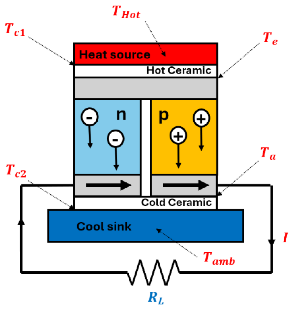
Figure 2.
Equivalent circuit of the coupled thermal and electrical system of the TEG.
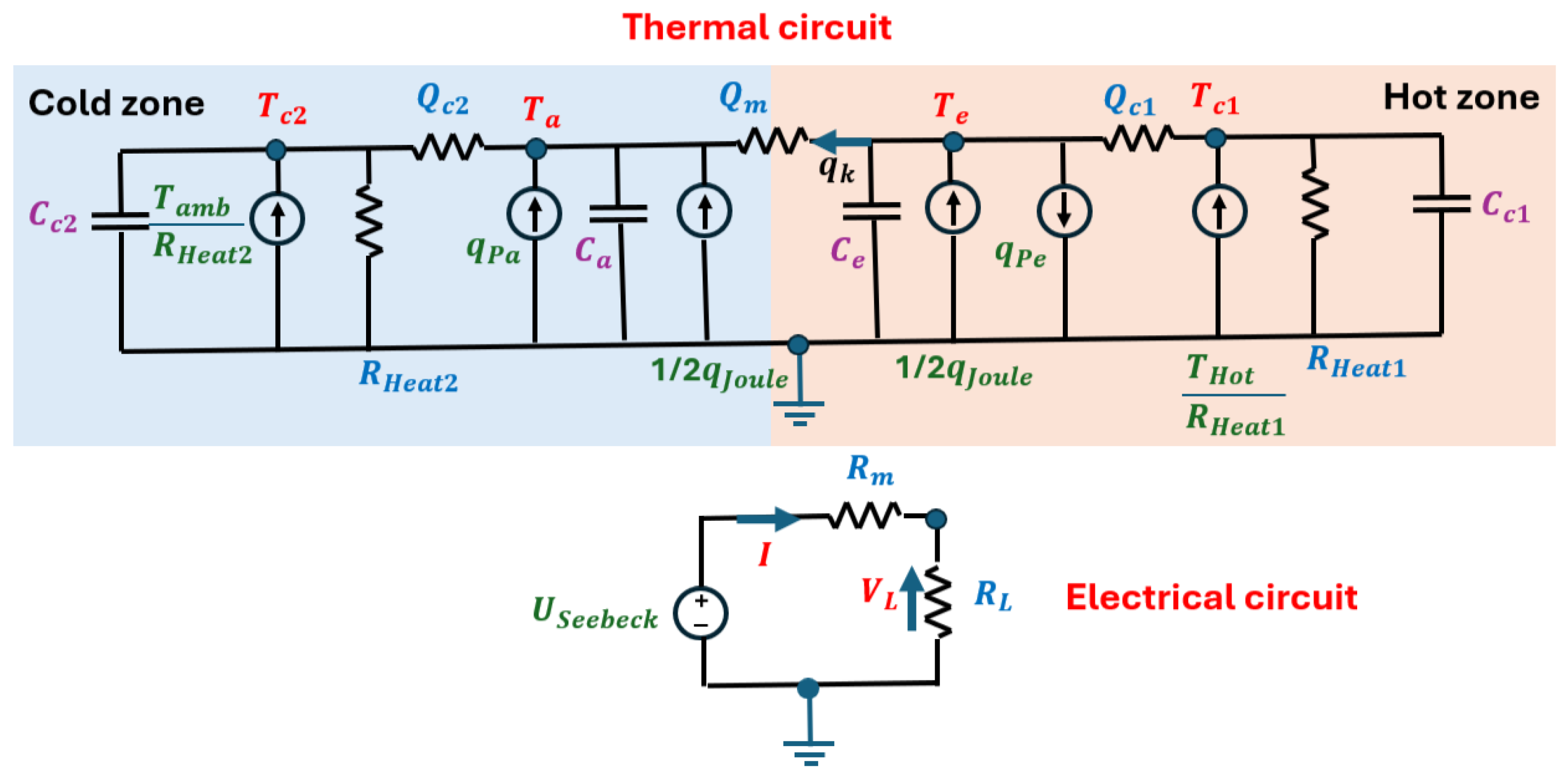
Figure 3.
Flowchart to obtain the expert model developed JanV1-4B-expert-TEG.
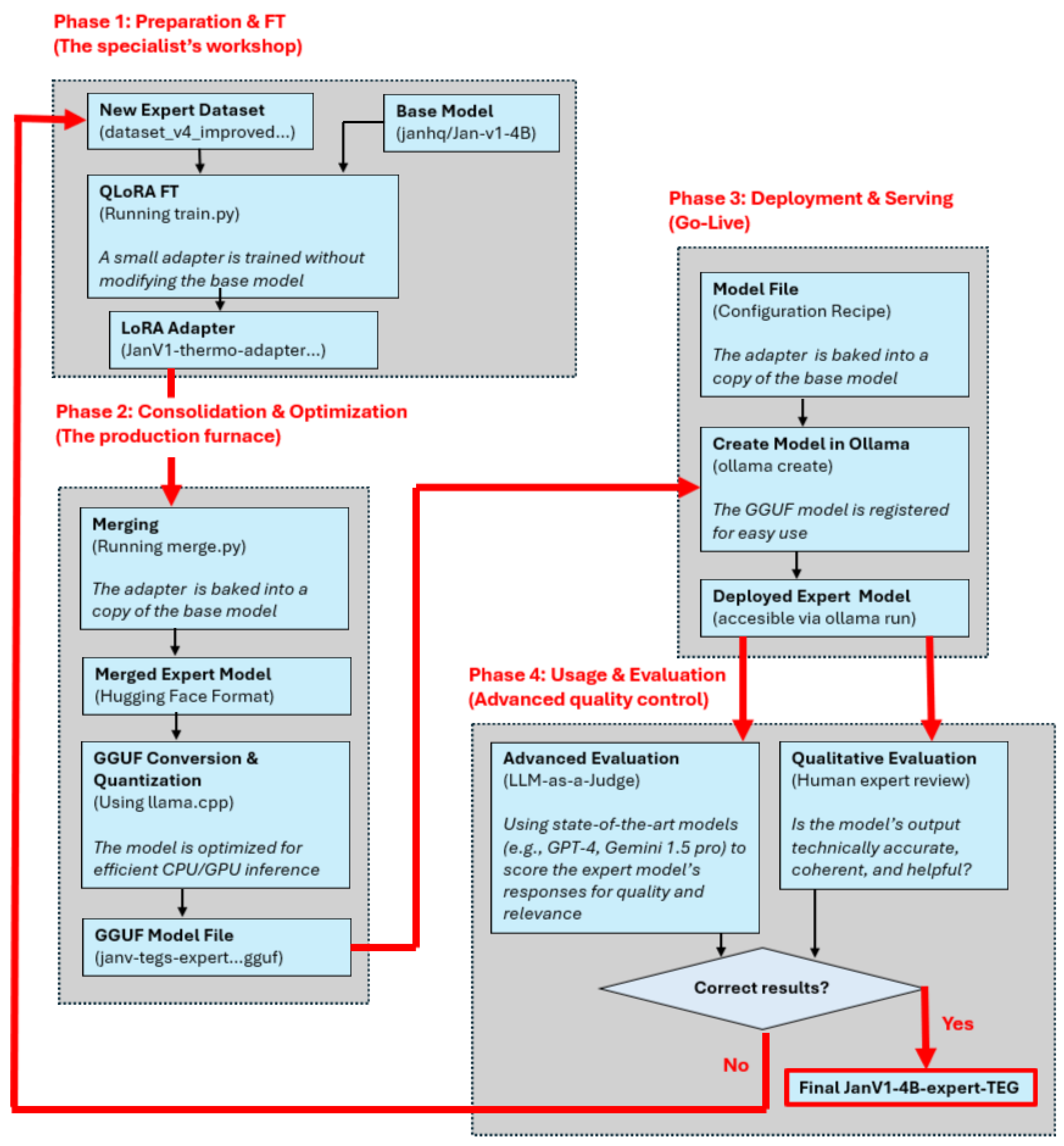
Figure 4.
Dataset flowchart.
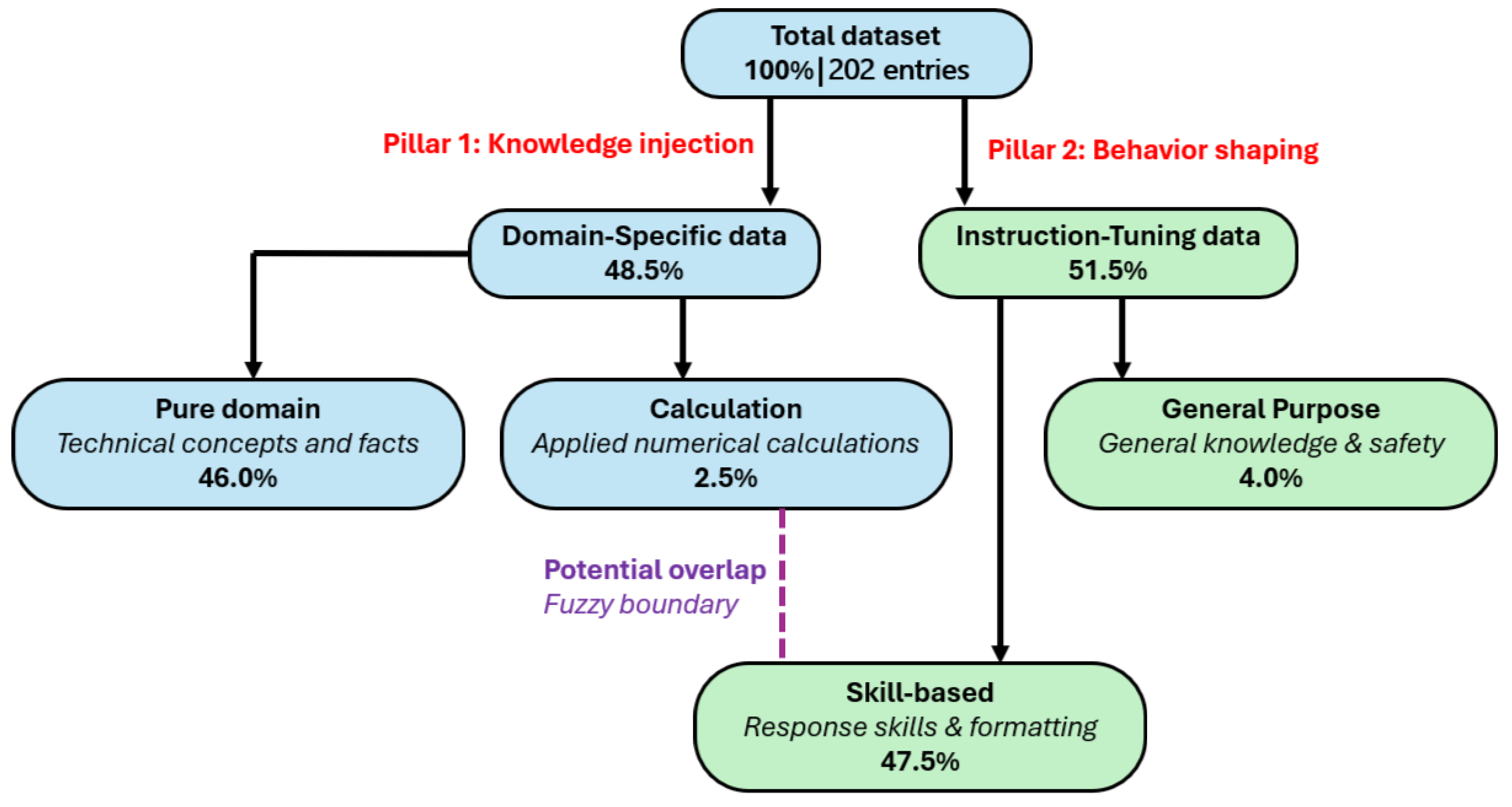
Figure 5.
Flowchart of the validation process for the LLM JanV1-4B-expert-TEG. The LLM demonstrates high performance and domain-specific reasoning.
Figure 5.
Flowchart of the validation process for the LLM JanV1-4B-expert-TEG. The LLM demonstrates high performance and domain-specific reasoning.
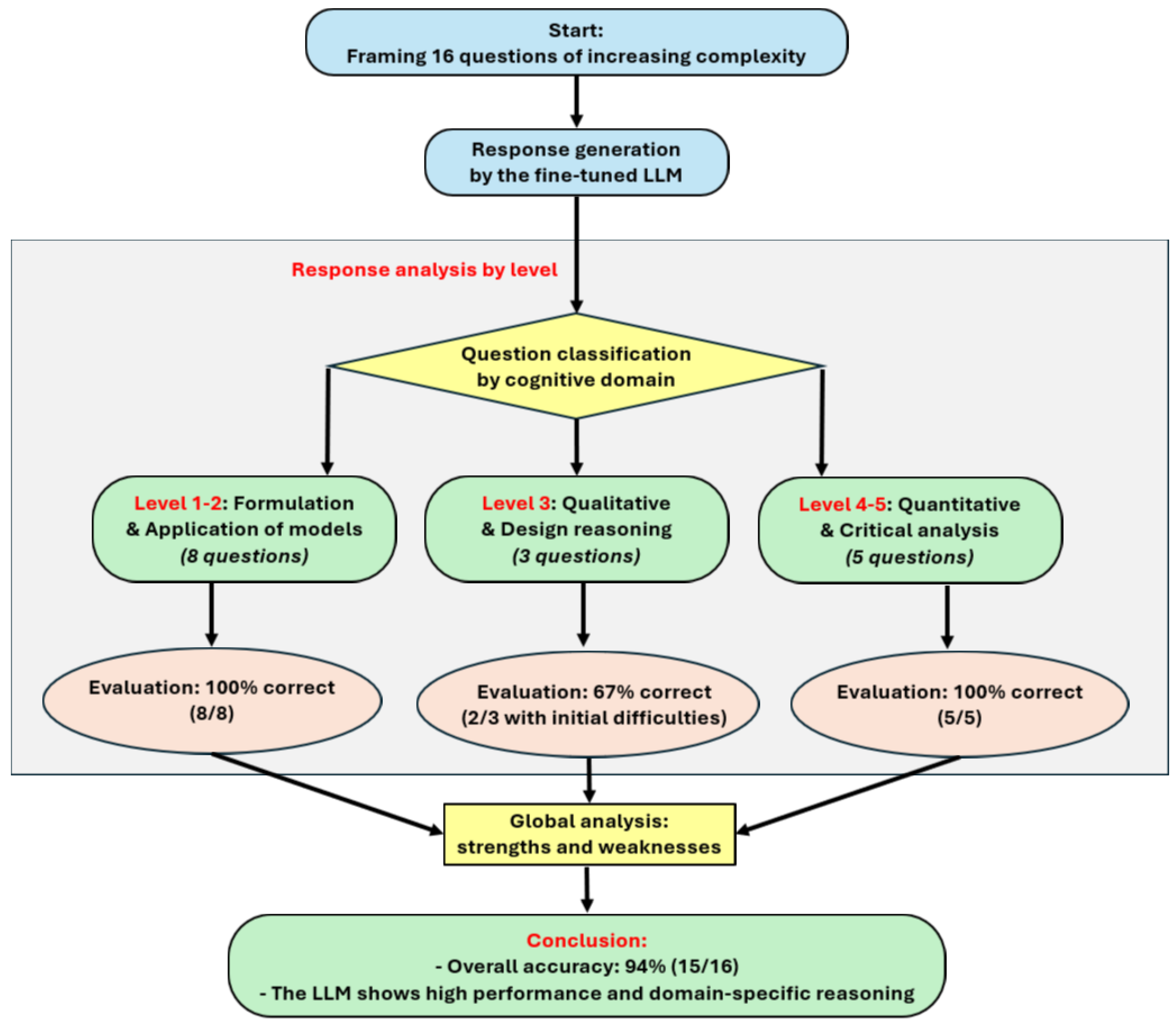
Figure 6.
Comparative analysis of the two specialized FT models, JanV1-4B-expert-TEG and Qwen3-4B-thinking-2507-TEG, against five other generalist base models.
Figure 6.
Comparative analysis of the two specialized FT models, JanV1-4B-expert-TEG and Qwen3-4B-thinking-2507-TEG, against five other generalist base models.
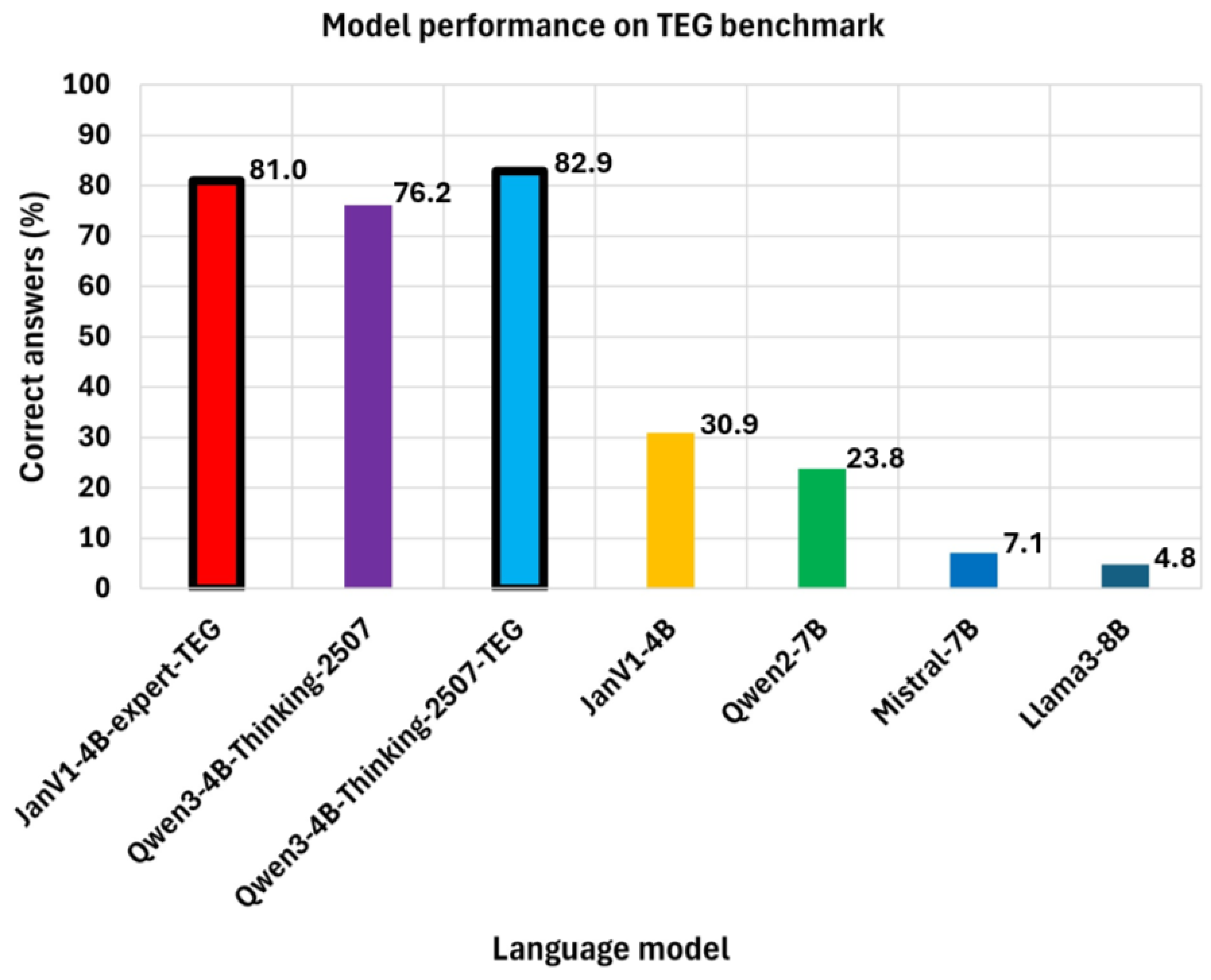
Figure 7.
a) Experimental design of the TEG and measuring devices. b) Arrangement of the 10 Peltier cells.
Figure 7.
a) Experimental design of the TEG and measuring devices. b) Arrangement of the 10 Peltier cells.
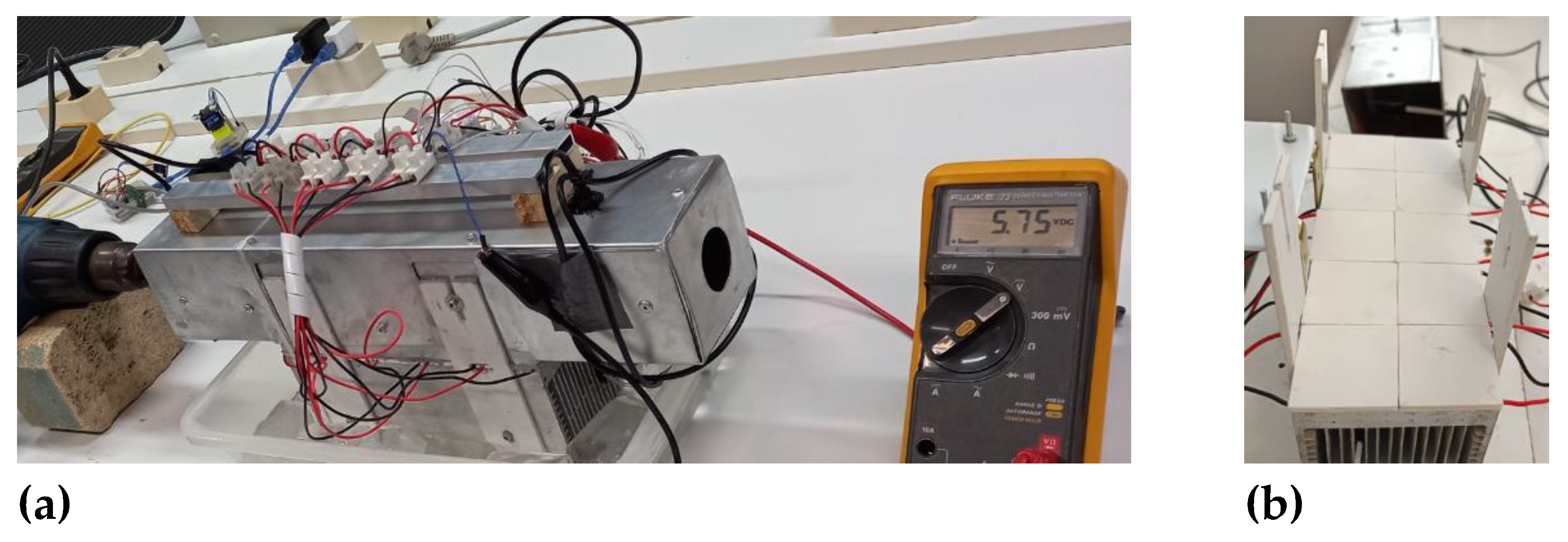
Figure 8.
Temperature profile on the upper and lower faces at the Peltier cell inlet and outlet, temperatures at the inlet and outlet of the upper heat sink, and ice temperature of the lower heat sink.
Figure 8.
Temperature profile on the upper and lower faces at the Peltier cell inlet and outlet, temperatures at the inlet and outlet of the upper heat sink, and ice temperature of the lower heat sink.
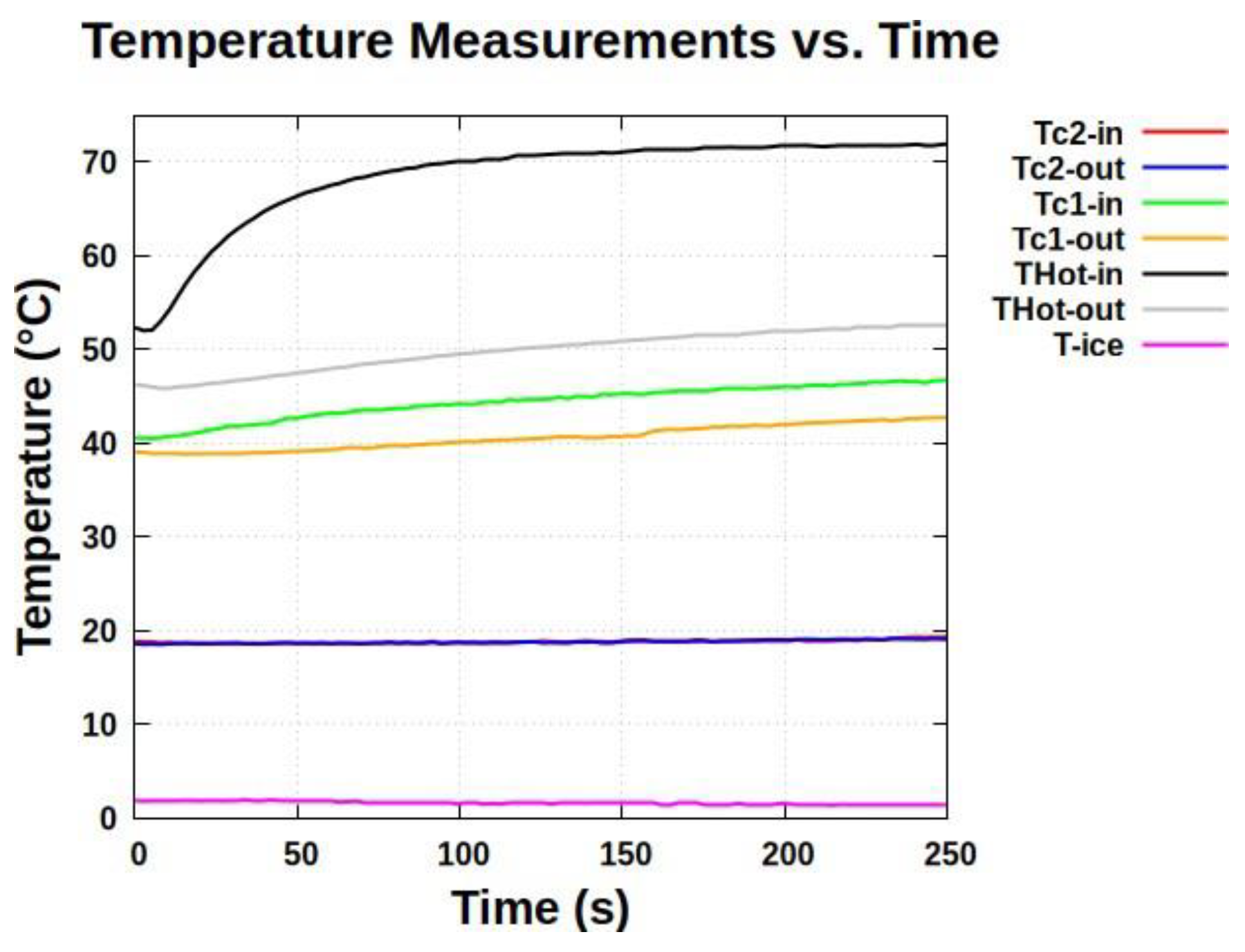

Table 1.
Magnitudes and physical properties of the TEG lumped parameter model.
| Symbol | Name | Unit |
|---|---|---|
| Temperature on the inner surface of the cold face. | K | |
| Temperature on the outer surface of the hot face. | K | |
| Temperature on the outer surface of the cold face. | K | |
| Temperature on the inner surface of the hot face. | K | |
| Cold source temperature. | K | |
| Hot zone temperature. | K | |
| Peltier heat flow sink at node . | W | |
| Peltier heat flow source at node . | W | |
| . Joule heat flow. | W | |
| . Heat flow by conduction between and . | W | |
| Seebeck coefficient. | V/K | |
| Internal electrical resistance of the module. | ||
| Thermal resistance by conduction. | K/W | |
| Thermal resistance of the ceramic on the hot face. | K/W | |
| Thermal resistance of the ceramic on the cold face. | K/W | |
| Thermal resistance of the heat sink on the hot face. | K/W | |
| Thermal resistance of the heat sink on the cold face. | K/W | |
| Thermal capacitance of node of the inner hot face. | J/K | |
| Thermal capacitance of node of the inner cold face. | J/K | |
| Thermal capacitance of the ceramic on the hot face. | J/K | |
| Thermal capacitance of the ceramic on the cold face. | J/K | |
| Resistance of the external electrical load. | ||
| Electric current generated that circulates through the circuit. | A | |
| Voltage generated at the load terminals . | V | |
| . Seebeck voltage. | V |
Table 2.
Classification and quantification of the 202 QA of the dataset.
| Classification | Quantity | (%) | Main objective and justification |
|---|---|---|---|
| Pure domain | 93 | 46.0 | To inject factual knowledge, theoretical knowledge and terminology from the field of thermoelectricity. |
| Calculation | 5 | 2.5 | To teach the model to apply domain-specific mathematical formulas to solve practical problems. |
| Skill-based | 96 | 47.5 | To teach a behavior. How to structure complex responses consistently to a variety of instructions, especially equations. |
| General Purpose | 8 | 4.0 | To mitigate catastrophic forgetting, maintain the overall versatility of the model, and ensure that it does not become over-specialized. |
| 202 | 100.0 |
Table 3.
Summary and evaluation of the responses of LLM JanV1-4B-expert-TEG.
| Question | Main Topic | Level | Evaluation |
|---|---|---|---|
| 1 | Equation of the node on the outside of the hot face, | 1 | excellent |
| 2 | Equation of the node inside the cold face, | 1 | excellent |
| 3 | Equation of the inner surface node of the internal hot face with Peltier and Joule effects, | 2 | excellent |
| 4 | Equations of the two internal junctions | 2 | excellent |
| 5 | Equations at the 4 nodes , | 2 | correct with difficulties |
| 6 | Cold side equations of the system | 2 | excellent |
| 7 | Open electrical circuit scenario =0 | 2 | excellent |
| 8 | Interpretation of the term storage | 1 | excellent |
| 9 | State variable format: solving the derivate | 1 | excellent |
| 10 | Combined conceptual balance of internal nodes | 3 | excellent |
| 11 | Steady-state equation at a node | 1 | excellent |
| 12 | TEG leg geometry: trade-off | 3 | correct with difficulties |
| 13 | Material selection and merit figure ZT | 4 | excellent |
| 14 | Geometry and contact strength | 4 | excellent |
| 15 | Temperature-dependent properties | 4 | excellent |
| 16 | Interpretation of simulation results | 4 | excellent |
Table 4.
Evaluation of parameters with different optimization algorithms.
| Algorithm |
Time (s) |
Final error |
(V/K) |
() |
(K/W) |
(K/W) |
(K/W) |
(K/W) |
| GA | 1128.76 | 0.00291 | 0.0171 | 2.4457 | 20.8545 | 0.0759 | 0.2379 | 0.0890 |
| GAN | 1235.58 | 0.00276 | 0.0151 | 2.0669 | 23.0098 | 0.0833 | 0.0941 | 0.0988 |
| DE | 108.90 | 0.00288 | 0.0155 | 1.9940 | 24.0509 | 0.0875 | 0.4778 | 0.1035 |
| SHGO | 6.67 | 0.56488 | 0.3496 | 5.0000 | 15.0500 | 0.0111 | 1.0000 | 0.0133 |
Table 5.
Comparison between experimental and simulated temperatures.
| (°C) | Data source | (°C) | (°C) |
|---|---|---|---|
| Experimental | 1.079 | 19.076 | |
| GA | 1.078 | 19.092 | |
| 0.0 | GAN | 1.079 | 19.075 |
| DE | 1.078 | 19.080 | |
| SHGO | 1.081 | 19.088 | |
| Experimental | 86.030 | 23.288 | |
| GA | 85.994 | 23.279 | |
| 90.0 | GAN | 86.038 | 23.317 |
| DE | 86.033 | 23.291 | |
| SHGO | 86.170 | 23.216 |
Table 6.
Performance comparison of Qwen3-4B models [41].
Table 6.
Performance comparison of Qwen3-4B models [41].
| Benchmark | Qwen3-4B- Thinking-2507 | Qwen3-4B- Thinking | Qwen3-4B- Instruct-2507 | Qwen3-4B- Non-Thinking |
|---|---|---|---|---|
| GPQA [43] | 65.8 | 55.9 | 62.0 | 41.7 |
| AIME25 [44] | 81.3 | 65.6 | 47.4 | 19.1 |
| LiveCodeBench v6 [45] |
55.2 | 48.4 | 35.1 | 26.4 |
| Arena-Hard v2 [46] | 34.9 | 13.7 | 43.4 | 9.5 |
| BFCL-v3 [47] | 71.2 | 65.9 | 61.9 | 57.6 |
Table 7.
Comparative summary of LLM performance and execution times in the TEG benchmark [21].
Table 7.
Comparative summary of LLM performance and execution times in the TEG benchmark [21].
| Model | Success | Errors |
Hit rate (%) |
Average time (s/answer) |
| Base model without FT | ||||
| Llama3-8B | 2 | 40 | 4.80 | 22 |
| Mistral-7B | 3 | 39 | 7.10 | 24 |
| JanV1-4B | 13 | 29 | 30.95 | 260 |
| Qwen3-4B-Thinking-2507 | 32 | 10 | 76.20 | 300 |
| Models with FT | ||||
| JanV1-4B-expert-TEG | 34 | 8 | 81.00 | 231 |
| Qwen3-4B-Thinking-2507-TEG | 34 | 7 | 82.90 | 486 |
Table 8.
Comparison of performance in general benchmarks of reasoning and creativity [6].
Disclaimer/Publisher’s Note: The statements, opinions and data contained in all publications are solely those of the individual author(s) and contributor(s) and not of MDPI and/or the editor(s). MDPI and/or the editor(s) disclaim responsibility for any injury to people or property resulting from any ideas, methods, instructions or products referred to in the content. |
© 2025 by the authors. Licensee MDPI, Basel, Switzerland. This article is an open access article distributed under the terms and conditions of the Creative Commons Attribution (CC BY) license (http://creativecommons.org/licenses/by/4.0/).
Copyright: This open access article is published under a Creative Commons CC BY 4.0 license, which permit the free download, distribution, and reuse, provided that the author and preprint are cited in any reuse.


