Submitted:
18 November 2025
Posted:
18 November 2025
You are already at the latest version
Abstract
Due to emerging strategic demands, this article presents a comprehensive conceptual design investigation into enhancing the MQ-9A Reaper Uncrewed Aerial Vehicle (UAV). Motivated by the need for persistent long-range strike and surveillance capabilities, the research study proposes three primary modifications to create an aircraft titled the MQ-9X Raven. First, we replace the existing turboprop engine with the widely used Williams FJ44-4A turbofan for fuel consumption and excess power at 50,000 feet, with a range of approximately 8000 nm. Second, we update the wing design with a 79 ft wing for a greater aspect ratio and a new LRN1015 airfoil to enable high-altitude, long-endurance standoff of around 24 hours. Third and finally, we integrate Joint Strike Missiles (JSM) for enhanced lethality. The project follows a rigorous methodology beginning with a redefinition of mission requirements, aerodynamic, thrust, and stability analysis, and then verification with flight simulation, computational fluid dynamics, and wind tunnel experiments. Our analysis shows the MQ-9X Raven is highly suitable for the task of pervasive high-altitude standoff maritime strike.
Keywords:
UAV
; flight testing
; simulation
; wind tunnel testing
; CFD
; missile
; stability
1. Introduction
In light of a deteriorating regional security environment and the growing emphasis on long-range precision capabilities, we propose enhancements to the MQ-9A Reaper to extend its operational range, safe operating altitude, and support alternative munitions configurations. Incorporating a persistent, armed ISR counterpart such as a MQ-9X Raven would bolster a host military’s ability to conduct integrated ISR-strike missions over extended distances, complementing existing assets and providing a responsive deterrent. The enhancement of the MQ-9A range, altitude, and payload flexibility aligns with strategic objectives to project power, protect National interests, and contribute meaningfully to allied operations in increasingly contested airspace.
The MQ-9X (Figure A1) is a heavily modified MQ-9A, with an upgraded engine to the Williams FJ-44A, increased wingspan to 79’, upgraded airfoil to the LRN1015 and Joint Strike Missile (JSM) weapon integration. This report does not justify the strategic security reasoning that motivate such modifications, only the implications on performance and mission effectiveness.
1.1. Background
In its current configuration, the MQ-9A Reaper is a single-engine turboprop, Medium-Altitude, Long-Endurance (MALE) Uncrewed Aerial Vehicle (UAV) capable of carrying 1361kg of external stores. It has a claimed ceiling of 50,000 feet, maximum speed of 240kts, and maximum endurance of 27 hours [1]. It can be equipped with an electro-optic/infrared (EO/IR) camera, a Lynx multi-mode RADAR, electronic support measures (ESM), and a laser designator. These capabilities make the Reaper a highly versatile multi-mission Intelligence, Surveillance, Targeting, and Reconnaissance (ISTAR) and strike aircraft. While the Reaper is highly versatile, it is less capable in a peer-to-peer strategic environment where it primarily flies at medium altitude, is required to reduce its altitude to release weapons, and flies relatively slowly.
1.2. Objectives
This report explores potential modifications and redesigns of the existing MQ-9A Reaper to better align with dynamic strategic contexts. It consists of a mission redefinition, analytic analysis, simulation analysis, CFD verification, and indicative wind tunnel testing.
2. Mission Redefinition
In order to meet more contemporary strategic outcomes as previously discussed, including the rise of generative AI, increasing proxy wars, and competing Global superpowers, a modernised MQ-9A Reaper mission is required. This new mission statement is defined as:
"Conduct persistent, long-range, high-altitude Intelligence, Surveillance, and Reconnaissance and long-range strike to deliver timely, accurate, and actionable intelligence and effects in support of strategic objectives" Subsequently, a redefined mission profile was generated as shown in Figure 1. This mission consists of a persistent high-altitude mission at 45,000’ with 12 hours of cruise time and weapons release before returning to base.
This redefined mission profile consists of a climb to the cruise altitude of 50,000’. The climb rate was set at >2000ft/min as can be accomplished by the Predator B [2]. The aircraft would then maintain this altitude to reduce the likelihood of detection and threat of ground-launched missiles. Maintaining this altitude improves flight efficiency by reducing the need to descend and climb for mission requirements. At a redefined cruise speed of 130KIAS (300KTAS), the 6-hour cruise leads to a 1800nm operational radius before weapons release. This mission profile (summarised in Table A1) lends the new aircraft to be a suitable maritime patrol and Anti-Access/Area-Denial (A2/AD) companion to the MQ-4C Triton and P-8 Poseidon. With this newly redefined mission statement, we developed more detailed mission and aircraft requirements.
3. Theoretical and Statistical Analysis
We performed an initial theoretical and statistical analysis of the MQ-9X, including weight and size, stability, mass properties, engine analysis, and airframe observability characteristics, in order to conduct a deeper analysis, including dynamic stability and simulations.

Table 1.
Weight Estimates for the MQ-9X Raven.
| Component [Text Method] | Abbreviation | Mass [lb] |
|---|---|---|
| Fuselage [3,4] | . | |
| Main Landing Gear (MLG) [4] | ||
| Nose Landing Gear (NLG) [4] | ||
| Nacelle [4] | ||
| Installed dry engine [4,5] | ||
| Fuel system [4] | 598 | |
| Furnishings [4] | ||
| Wing [6,7] | 1067.6 | |
| Empennage [6] | 120.5 | |
| Actuators [6,8] | 29.4 | |
| Flight controls [6] | 210.9 | |
| Electrical [6] | 131.3 | |
| Avionics [6] | 392.4 | |
| Anti-icing [9] | 88.2 | |
| Lightening protection [10] | 44.33 |
3.1. Weight and Size Analysis
In order to further verify some of the weight estimates, a comparison was made to an MIT paper Valuation Techniques for Commercial Aircraft Program Design [11] where wing and empennage weight are typically 23 and 3% of aircraft empty weight [11], or lbf (511.20 kg), and lbf (66.68 kg); an increase of 5.6% and 5.4% to above estimates. Therefore, the estimated weights calculated for both the wing and empennage were assessed as sufficiently accurate.
3.2. Mass Properties
The mass properties of each major component (fuselage, wing, empennage, landing gear, engine, payload, and pylons) were estimated based on a Fusion 360 model. For each of the four loading configurations (Maximum Take-Off Weight (MTOW), Full Fuel Zero Payload, Full Payload Zero Fuel, and Empty Weight), the x, y, and z coordinates of the CoG were obtained by summing the component moments about each axis. The computed values were compared against Fusion 360 outputs to validate the distribution.
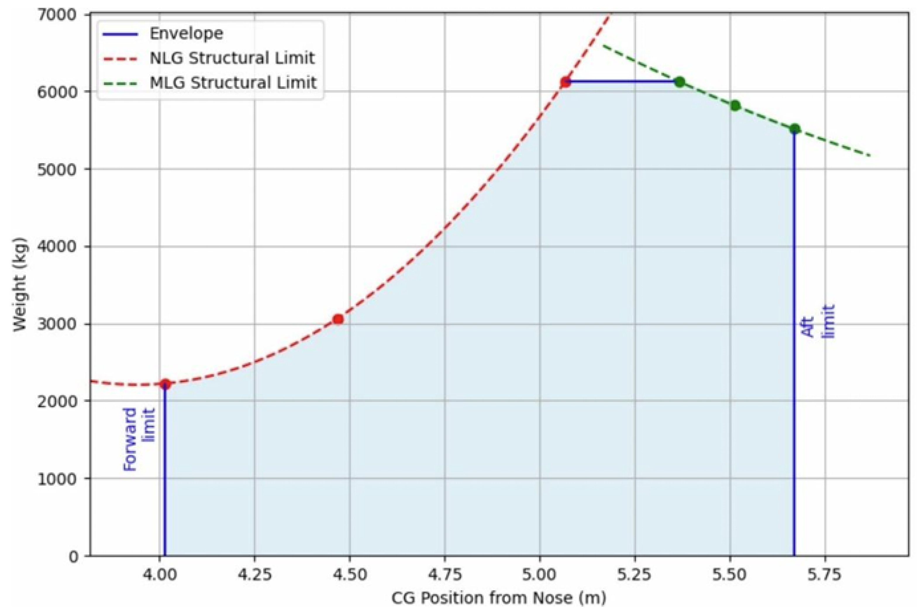
To determine the forward and aft CoG limits, moment-based estimations were performed using known main and nose landing gear load fractions. Following Gudmundsson [4], the forward limit was defined by the nose landing gear supporting approximately of the MTOW, while the aft limit corresponded to of the main landing gear bearing load. Applying these criteria yielded a forward limit at 4.015 m from the nose and an aft CoG limit at 5.511 m from the nose. Structural limit curves for both NLG and MLG were then plotted to form the CoG envelope boundary at Figure A6.
Previous Moments of Inertia (MoI) studies by the research team using the DATCOM method revealed results that aligned with the Fusion 360 model, so long as density estimates were transferred based on volume. Therefore, for each loading configuration, the MoI were extracted from the Fusion 360 assembly. The empty weight case was then compared with the previously validated DATCOM estimate for the 66 ft baseline, to ensure consistency. Across configurations, , , and decrease with total mass. For the empty weight case, comparison of the earlier 66 ft variant to the current 79 ft model shows a reduction of from m2 to 15013 m2 (48.56% decrease), an increase of from 9540 m2 to 12735 m2 (33.50% increase), and a reduction of from 37491 m2 to 27233 m2 (27.35% decrease). There is a mass contraction toward the longitudinal and lateral axes (lower and ) with a relative aft redistribution about the pitch axis (higher ). These trends imply reduced roll and yaw inertia but increased pitch inertia for the updated configuration, and that the Fusion 360 values are suitable for initial dynamic stability and control analyses.
3.3. Performance Analysis
3.3.1. Engine Type, Number and Sizing
The Raven is required to cruise at Mach 0.52 at an operational ceiling of approximately ft. In this regime, turboprops offer high propulsive efficiency at low Mach numbers but are fundamentally thrust-limited in the very low-density environment at altitude. Thrust and drag assessments and simulation indicated turboprops cannot sustain steady level flight at ft. Best suited to the flight regime is a high-bypass-ratio (HBR) turbofan; however, there would be significant integration challenges on the Raven due to larger fan diameters and nacelle volume. Consequently, a low bypass ratio (LBR) turbofan emerges as the practical solution.
The Williams FJ44-4A satisfies the altitude requirement and provides suitable thrust margin for the configuration. Prior work by the design team identified a minimum thrust requirement of approximately kN. The FJ44-4A is capable of delivering kN at takeoff (5 min) and kN continuous, exceeding the requirement. Integration of a LBR turbofan had been historically demonstrated for the prototype aircraft, Predator B [12,13], using the Williams FJ44-2A. Additionally, it was demonstrated in simulation for both the 66 ft baseline and the updated 79 ft wing configuration. While operation at Mach 0.5 is below the engine’s ideal cruise regime, the altitude capability and available thrust dominate the trade for long-range strike and surveillance aircraft.
An installed FJ44-4A already produces adequate thrust for the aircraft loaded with JSMs. Moving to a twin configuration would introduce penalties in mass, nacelle and interference drag, structural reinforcement, and duplicated systems, while complicating CoG management and increasing acoustic and IR signatures. Additionally, there is less operational need for propulsion redundancy in an uncrewed system. Consequently, the single-engine arrangement was retained. Rubberised engine sizing approaches were considered; however, for a high-altitude maritime strike platform where operational reliability outweighs optimisation, the fixed engine method was retained.
3.3.2. Fuel Consumption
Fuel consumption was a critical determinant of the Raven’s overall mission endurance and range capability. At the design cruise condition of Mach 0.5 and 50,000 ft, the low-bypass turbofan operates off its peak efficiency range, incurring a moderate increase in thrust-specific fuel consumption (TSFC). The selected Williams FJ44-4A has a published TSFC of approximately 0.485 lb/lbf/hr at its design point, which provides a realistic basis for endurance and range estimation when applied to the Raven’s low-Mach, high-altitude flight regime.
The aircraft’s total fuel capacity of 6,000 lb (2,720 kg) establishes a substantial energy reserve for extended missions. Applying the Breguet endurance and range relationships using the fixed FJ44-4A performance data yields an estimated endurance of approximately 28 hours and a corresponding range near 8,000 nmi.
3.3.3. Thrust-to-Weight Versus Wing Loading
Following the propulsion and structural updates to the Raven, the thrust-to-weight () and wing loading () characteristics were recalculated to establish a revised design point. The increase in wingspan from 66 ft to 79 ft increased the total wing area from 25.35 m2 to 28.66 m2, while the maximum take-off weight increased from 4672 kg to 6124 kg. Despite the larger lifting surface, the proportional weight growth produced a higher effective wing loading, shifting the design point toward a denser, higher-performance configuration.
The updated analysis produced a design point of , compared with the MQ-9 Reaper baseline value of . This shift reflects a substantial performance enhancement. The increase in results primarily from replacing the Honeywell TPE331-10 turboprop with the Williams FJ44-4A turbofan, which delivers higher thrust at altitude and supports greater climb and cruise performance. The higher value indicates an aircraft optimised for faster cruise and improved aerodynamic efficiency at altitude, though with higher stall speed and reduced take-off and landing margins.
When compared with contemporary long-endurance UAVs, such as the Hermes 900, Predator XP, CH-4, Gray Eagle, and Wing Loong II, the Raven occupies the endurance-optimised region of the – scale. The resultant configuration of the Raven is well aligned with its intended Maritime Strike mission profile, combining efficiency and operational flexibility while maintaining adequate excess power for altitude and payload demands.
3.3.4. Thrust Available Versus Thrust Required
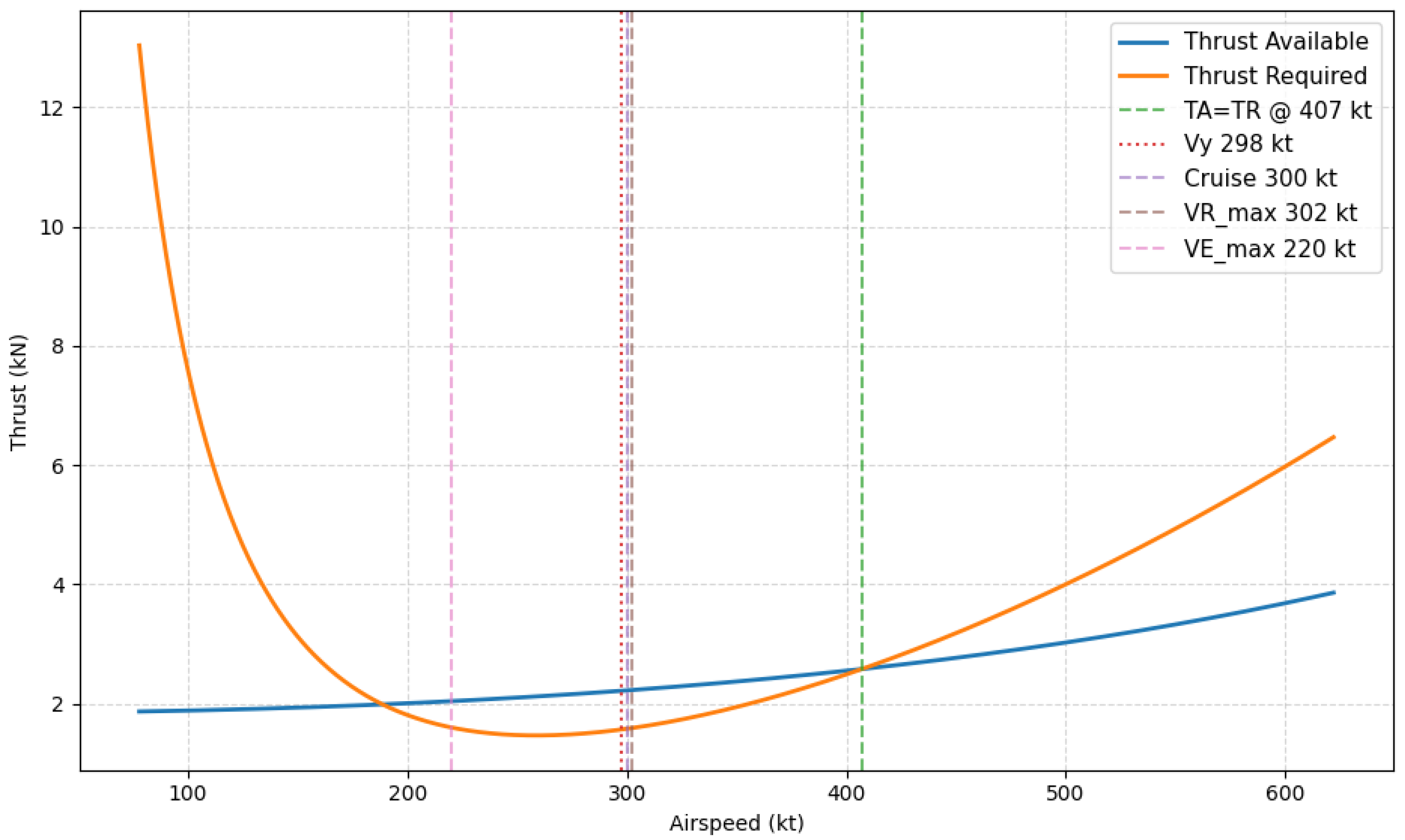
A thrust analysis was performed to compare the Raven’s thrust available (TA) from the Williams FJ44-4A turbofan against the thrust required (TR) for steady level flight across the speed range at the design altitude of 50,000 ft. The TA curve (Figure A5) was derived from standard atmosphere scaling laws for a low-bypass turbofan, while TR was computed from the aerodynamic drag polar using the updated wing geometry and configuration parameters, at MTOW. This provided direct insight into the aircraft’s ability to sustain flight, climb, and cruise at its operational ceiling.
The resulting TA-TR plot indicated that the cruise speed (300 kt), maximum range speed (302 kt), and best rate-of-climb speed (298 kt) all converge within a narrow band near the region of maximum excess thrust. This concentration demonstrates a well-balanced aerodynamic and propulsion design. The maximum endurance speed of approximately 220 kt corresponds to the minimum of the TR curve, representing the most fuel-efficient loiter condition but with a smaller thrust margin and limited climb performance. The intersection of the TA and TR curves occurs around 407 kt, defining the theoretical maximum level-flight speed at altitude. It was evident that the Raven has a sufficient thrust margin at its design cruise speed to maintain level flight at 50,000 ft with modest excess power available for further climb or manoeuvre.
3.3.5. Aircraft Drag Analysis
The zero-lift drag coefficient for the MQ-9 Raven was determined analytically following the methodology presented by Gudmundsson [14]. The total zero-lift drag coefficient without external stores, , is expressed as the sum of the non-wing parasite drag and the wing contribution:
Each component was derived using the appropriate aerodynamic calculations and geometric parameters from the MQ-9 Raven configuration [Appendix]. The subsequent analysis also accounts for the effect of six external stores, resulting in an adjusted drag model and refined cruise drag estimate.
The non-wing parasite component was obtained from Zountouridou et al. [15]. The wing contribution, , was calculated using the method defined by Gudmundsson [14], incorporating the wetted-area ratio, skin-friction coefficient, form factor, and interference factor. With , , (from Torenbeek [9]), and , the wing contribution was found to be . Hence, the total zero-lift drag coefficient without stores was .
The MQ-9 Raven is capable of mounting six external stores, distributed symmetrically beneath the wings. The aerodynamic contribution of these stores to overall drag was estimated using the findings of Manaf et al. [16], who experimentally observed a 4% increase in per store pair under comparable subsonic conditions. For three store pairs, this corresponds to a 12% increase in total parasite drag, yielding . To model the variation of drag with lift coefficient, the adjusted drag method from Gudmundsson [14] was employed:
Here, , with e representing the Oswald efficiency factor and the aspect ratio. Based on interpolation of the LRN 1015 airfoil data in Hicks and Cliff [17], the value of was determined to be approximately . For a representative cruise lift coefficient of and the adjusted zero-lift drag coefficient , the resulting total drag coefficient was .
The corresponding drag force for the MQ-9 Raven under cruise conditions at 50,000 ft was computed using the standard drag equation With , , , and , to be a total drag of D(stores) = 2342.36 N.
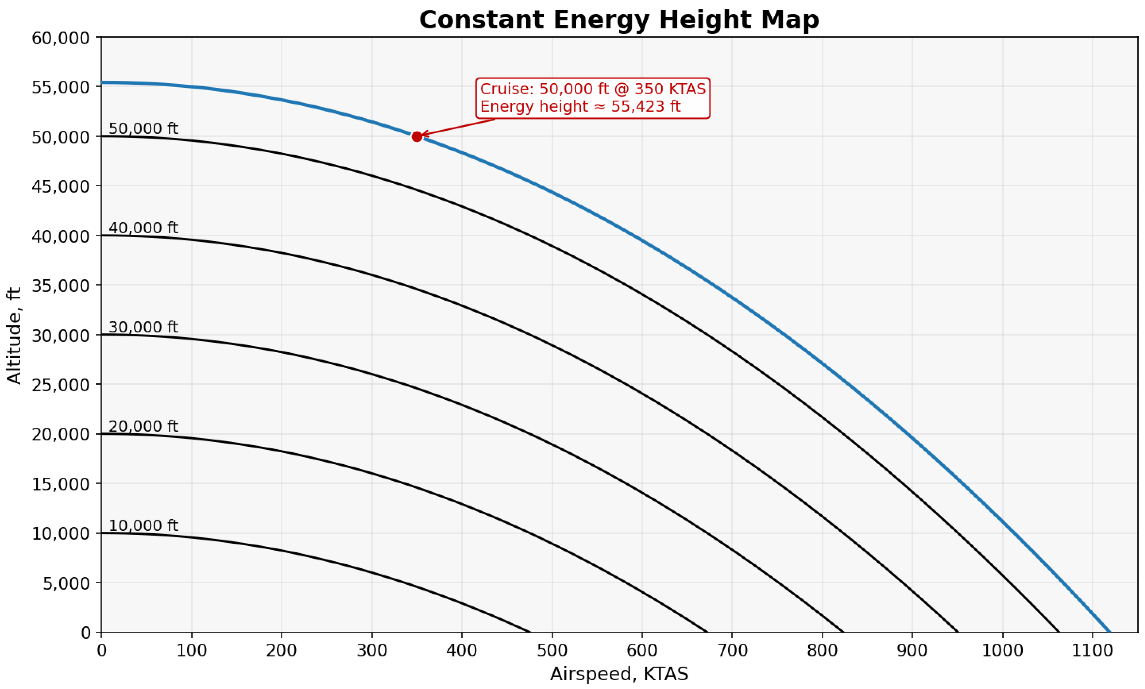
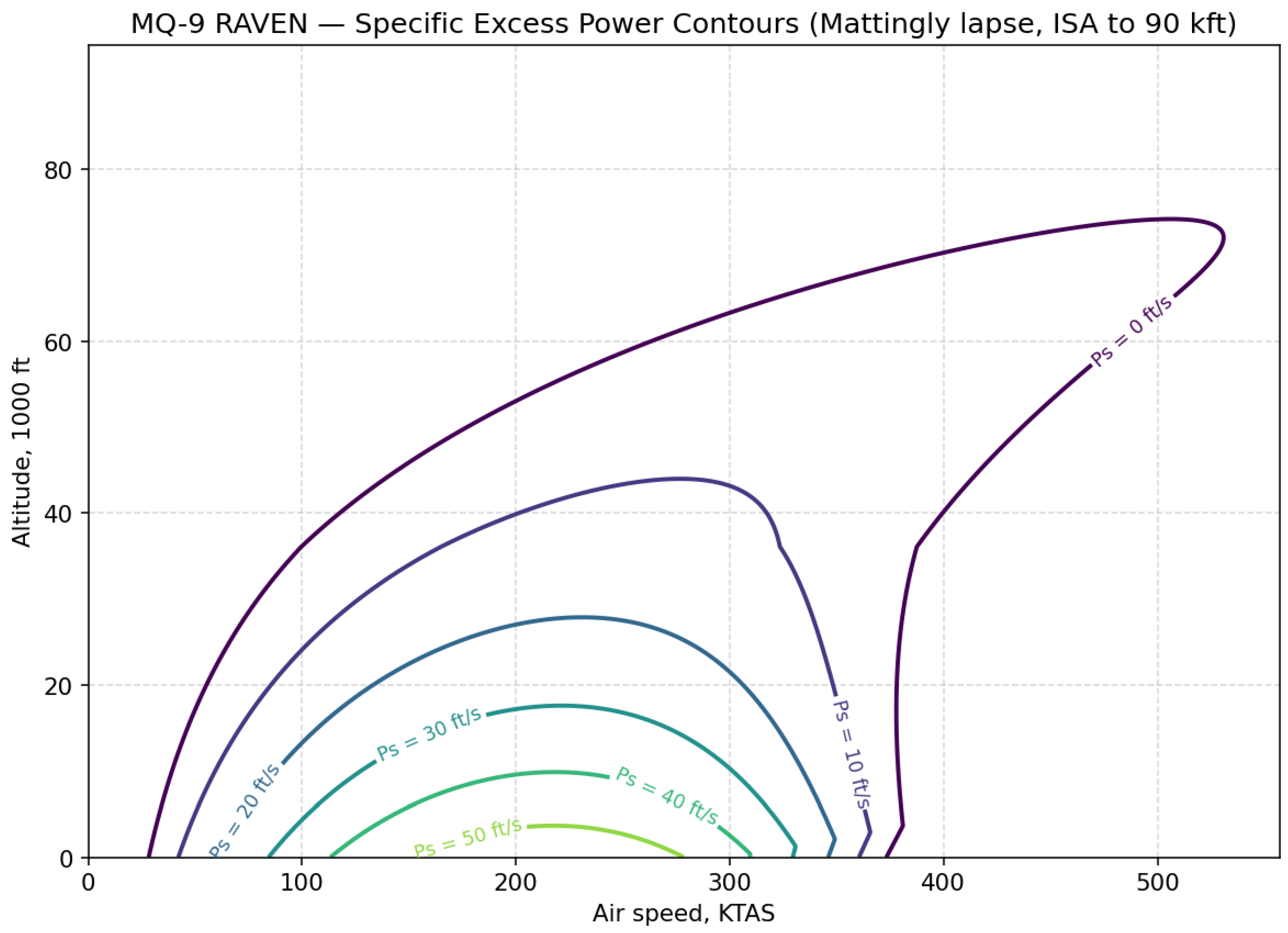
A detailed Constant Energy Height Map [Annex C, Figure A2] and the corresponding Specific Excess Power Contours [Annex D, Figure A3 & Figure A4] are presented in the Annex. These figures illustrate the MQ-9 Raven’s energy performance characteristics across its operational flight envelope, providing insight into the aircraft’s climb capability, acceleration potential, and overall energy manoeuvrability during sustained flight conditions.
3.3.6. Engine Characteristics
The maximum engine mass flow rate for the Williams FJ44-4A turbofan is not publicly available. Therefore, it was estimated using the method described by van Kuik [18]. Engine parameters and take-off performance data were obtained from the type-certification data sheet [19] and supporting manufacturer documentation [20], with atmospheric properties defined by the ISA standard [21]. At static take-off conditions (, , ), the calculated mass flow rate is . For cruise at 50,000 ft (, , ), the mass flow rate reduces to . As the MQ-9 Raven uses an off-the-shelf Williams FJ44-4A installation [22], the inlet design parameters remain consistent with published manufacturer data.
The inlet face and compressor front are co-located and thus share identical geometry. Therefore, the inlet velocity for both flight conditions is determined using the same effective area. At static take-off, the inlet velocity is , corresponding to a Mach number of using a sea-level speed of sound of . At cruise altitude, the inlet velocity increases slightly to , yielding based on . Both conditions confirm that inlet flow remains subsonic across the entire flight envelope.
Flow properties were determined at the inlet station (Station 1) for both operating conditions using standard relations [18,21]. For static take-off, the total pressure, temperature, and density are , , and , respectively. At cruise altitude (50,000 ft), the corresponding parameters are , , and . A comparison between far-field (Station 0) and inlet (Station 1) conditions for both regimes is summarised below.
Table 2.
Summary of Flow Conditions at Engine Inlet
| Condition | Altitude | (N/m2) | (K) | (kg/m3) | |
|---|---|---|---|---|---|
| Static Take-Off | SL | 0.42 | 255.3 | 1.23 | |
| Cruise | 50,000 ft | 0.51 | 181.1 | 0.187 |
The results validate the aerodynamic compatibility of the Williams FJ44-4A engine with the MQ-9 Raven configuration across its operational flight envelope.
3.3.7. Observability Analysis
Observability can be considered in three main areas of acoustics, infrared, and radar.
The MQ-9 Reaper’s turboprop produces a distinct low-frequency buzz easily recognised by ground observers [23]. Replacing the turboprop with the FJ44-4A turbofan introduces higher-frequency broadband noise and fan tones [24], which weaken much more rapidly with distance [25]. The engine position on the Raven provides additional airframe shielding [26], while the mixed-flow nozzle and acoustic liners reduce jet noise by up to 5 dB [27,28]. These modifications make the Raven notably quieter and less distinct than the Reaper, particularly at altitude.
The FJ44-4A’s bypass design lowers the core temperature by mixing cool bypass air with the exhaust [27]. However, the absence of propeller wash yields a more concentrated plume [29]. The upward-facing exhaust, shielded by the fuselage and wing, reduces IR detectability from the ground [25]. Although less optimised than the Predator C Avenger’s S-duct configuration [30], the Raven achieves moderate IR suppression from below but remains more visible from above than the Reaper’s turboprop configuration.
The Raven retains most of the Reaper’s external geometry and stores capability, maintaining an estimated RCS of [29]. The exposed turbofan face increases reflections from upper and oblique angles, however, the removal of the propeller eliminates the main Doppler returns [31]. The top-mounted intake smooths the lower profile, reducing downward-hemisphere returns, though overall radar observability remains comparable to the Reaper.
3.4. Stability Analysis
Each of the main dynamic stability modes was estimated theoretically at the main cruise design point 50,000 ft (Mach ) before conducting simulations to confirm their magnitude and effects. Geometry, mass properties, and operating conditions were taken from the Reaper standard configuration [32], with atmospheric properties referenced to ISA [21].
3.4.1. Short-Period Approximation
The short-period dynamic response was assessed using stability-derivative formulations from Gudmundsson [6], converted to non-dimensional form following Nelson [33], and applied within Stengel’s [34] short-period expressions. Each of the short-period factors is summarised followed by an estimation of the natural frequency and damping.
- Non-Dimensional Longitudinal Derivatives: The resulting derivatives were: Pitch-rate derivative: ; Angle-of-attack rate derivative: ; Normal-force -derivative: ; and Pitching-moment -derivative: .
Substituting the above into Stengel’s short-period relations [34] gives the natural frequency and damping ratio , indicating a strongly damped short-period mode with a moderate natural frequency, consistent with the slender, high-aspect-ratio configuration and tail leverage embedded in the standard Reaper baseline [4,32,34].
3.4.2. Phugoid
The phugoid mode is characterised by a natural frequency and a dampening ratio . These values were found using small angle approximation [35] and the longitudinal stability derivatives and respectively (from [33]). At cruise condition these were calculated to be and . Therefore, and .
The natural frequency of the phugoid mode in aircraft dynamics typically ranges from 0.1 to 1 rad/s [36], with dampening ratio usually very low or near zero [36]. Therefore, the calculated natural frequency and dampening ratio both fall on the lower side of the acceptable range of these values; a phugoid trend typical in aircraft design at such high altitudes. As such, the aircraft is likely to experience slow, lightly damped longitudinal oscillations in response to disturbances in speed or altitude. A low natural frequency (≈ 0.0732 rad/s) gives a long-period oscillation seconds, whilst a low damping ratio (0.0167 (Level 2 Stability [37])) means that the oscillations will decay very slowly. As such, cyclic effects on the sensing, engine, and structure will likely need to be minimised by introducing an altitude hold autopilot on the aircraft.
3.4.3. Directional Stability
The directional stability of the Raven was determined using equations from chapters 24-25 of [6], with the primary intent of this analysis being the determination of . As the Raven has a Y tail and there are not Y tail-specific formulae, we initially took a simplified projection of the surfaces onto the vertical and horizontal planes, yielding a , which is within the range of 0.03 to 0.2 specified and is positive directional stability. The complexity of the empennage to get the computations correct and work on alternative arrangements led to Athena Vortex Lattice (AVL) [38,39] and VSPAERO [39] being independently used to check this estimate. For example, the VSPAERO analysis was inspired by [40] and involved the complete aircraft geometry being constructed in OpenVSP based on the dimensions of the team’s common CAD model. After an appropriate tessellation involving 3296 elements and appropriate convergence checks [39], sideslip values from to degrees were tested in 2-degree increments at the cruise angle of attack of 1.5 degrees and other cruise conditions. A relatively narrow range was selected because inviscid methods, such as VSPAERO, inherently do not model flow separation, which becomes more significant at higher angles of attack. The VSPAERO surface plot is shown at Figure 2 and the sweep regression at Figure 3, finding with an and an estimated uncertainty of . The AVL analysis of the aircraft, modelling only thin sets, yielded , two percent lower than the VSPAERO result. The relatively small difference is attributed to VSPAERO’s inclusion of thick-body effects and AVL’s omission of the nacelle.
3.4.4. Dutch Roll
The necessary non-dimensional stability derivatives for Dutch Roll were calculated from Chapter 24-25 of Gudmundsson et al [6], yielding: yaw moment to sideslip , yaw moment to yaw rate , and side force to sideslip . These were dimensionalised to the following using equations from [41] to then input to the equations given below from the same reference: sideforce to sideslip, ; yaw moment to sideslip, ; yaw moment to yaw rate, ; and sideforce to yaw rate, .
This analysis shows the Raven is very stable in the Dutch roll mode, with a high positive damping ratio and long duration period.
3.4.5. Dihedral Effect Analysis
The dihedral effect derivative, , was estimated by summing the contributions of the lifting and stabilising surfaces, namely the wing, V-tail, and ventral fin. The wing dihedral effect arises from its dihedral angle, twist distribution, and moderate sweep, for which the Raven’s wing has a negligible dihedral effect. The V-tail was modelled as a secondary wing, evaluating its dihedral effect in the same way and determining a strong contribution attributed to the dihedral angle. The ventral fin contributes a small destabilising dihedral effect due to the offset of its mean aerodynamic chord below the aircraft centreline, which shifts the restoring moment arm in the vertical direction during sideslip.
The component contributions and total dihedral effect are summarised in Table 3. The total dihedral effect for the MQ-9X Raven configuration was found to be . This exceeds the rule of thumb of about by 42%, suggesting that the MQ-9X possesses strong lateral stability. This characteristic enables the aircraft to naturally return to wings-level flight following a rolling disturbance, reducing the corrective workload on the pilot or autopilot system.
3.4.6. Roll Control and Dynamics
The roll control power, , was calculated by integrating the aileron effect across the span, accounting for a control surface effeciveness of estimated at the aileron semi-span [6]. The aileron control derivative was found to be .
The steady-state roll rate depends primarily on the roll control power, airspeed and roll damping. Approximating a first-order roll, at the 300 KTAS cruise condition, a aileron deflection would generate a steady-state roll rate of approximately /s, confirming moderate roll responsiveness despite the high aspect ratio. This provides adequate manoeuvrability for the mission needs, especially given that higher aileron deflections are available at lower speeds such as during takeoff and landing. The transient roll response after initiating an aileron deflection has a time constant between – s depending on the roll moment of inertia , as varied with changes in wing fuel and store loads.
4. Simulation
This section verifies the static and dynamic stability of the Raven through the use of two simulations. Austin Meyer’s xPlane 11 [42] and Mark Drela and Harold Youngren’s Athena Vortex Lattice (AVL) [43] were utilised for this simulation analysis.
4.1. Dynamic Stability
During early simulation experimentation within xPlane, it was discovered that at the desired cruise altitude the Raven had noticeable and undesirable phugoid motion, which made it difficult to fly straight and level. This phenomenon led to further analysis to determine the root cause, and the creation of two candidate tail variants to potentially improve dynamic stability behaviour.
The tail variants, shown in Figure 4, are screen captured from xPlane, identical models also created in AVL for a direct comparison. For simulation verification, the 3D lift slopes of both methods were compared to the theoretical three-dimensional (3D) lift slope Chapter 9 [6]: 3D theoretical, , 3D AVL and 3D xPlane . This equates to a 4.7% difference between theoretical and AVL and a 7.6% difference between theoretical and xPlane.
Next, static stability of the tail configurations was determined by plotting versus , with positive stability determined with a positive and negative . The results in Figure 5, show all 3 tail variants are stable for longitudinal static stability.
Since, the tail variants lead to a statically stable Raven, we continued with dynamic stability analysis. To achieve this, we built a custom Python script to execute the flight test regimes following the procedures from Air Force Flight Test Center [37]. The results of these experiments are shown in Table 4 while an example generated output simulation is shown at Figure 6.
The damping ratio and natural frequencies are further analysed by determining the flying qualities from [37] as shown in Table 5.
The standard Reaper tail configuration applied to the Raven yields the best results, with only a Level 2 in Phugoid as expected. This investigation resulted in a fourth tail variant experiment consisting of a standard Reaper tail with 150% surface area increase. The area increase was accomplished by increasing only the chord of the tail surface. This fourth configuration resulted in and , which is Level 1 in the Phugoid mode. The larger tail is recommended.
4.2. Joint Strike Missile Integration
The integration of the JSM onto the MQ-9 platform was investigated to expand its stand-off strike capability. The JSM, designed by Kongsberg Defence & Aerospace, is an air-launched, long-range, low-observable cruise missile optimised for low-altitude sea-skimming flight [44]. Achieving this mission profile requires careful consideration of aerodynamic trim, control, and stability.
A weapon integration test plan was constructed in order to identify the processes involved with integrating JSM’s onto the MQ-9 platform. The plan provides the tests and simulations required to achieve certification and clearances from appropriate organisations, as seen in Table A2 of Appendix E. As a precursor to early safe separation analysis from the Raven, a limited study was conducted into the JSM’s aerodynamic coefficients and stability using AVL software [43] per the analysis objectives in Table 6 and the workflow in Table 7.
A symmetric NACA-0012 airfoil was assumed for the simulation. The reference area, span, and mean aerodynamic chord (MAC) were defined based on open-source photographic geometry. Static stability was assessed by plotting the pitching moment coefficient () versus angle of attack () over an sweep, with results seen in Table 8. Although the missile is statically stable, the small static margin suggests potential sensitivity to disturbances.
Trim searches at three key altitudes are shown in Table 9 that indicate that the JSM cannot be trimmed at high altitude and low dynamic pressure conditions typical of the MQ-9X Raven cruise without extreme angles of attack. Further, sea-level Mach 0.9 conditions yield a practical and efficient trim consistent with the missile’s sea-skimming design. These characteristics would require the JSM to dive to sea level before beginning steady-level flight. The characteristics also necessitate further study on the pitch stability in the ejected safe separation conditions and during dive.
Dynamic stability was assessed from the trimmed sea-level condition using AVL’s eigenmode analysis. The missile exhibited three primary longitudinal and lateral-directional modes, seen in Table 10. These results indicate that while the JSM is dynamically stable in pitch, it may require yaw damping augmentation (e.g., via control law tuning) to suppress Dutch Roll oscillations.
AVL’s linear and inviscid assumptions make it suitable for conceptual design but limit accuracy for high angles of attack or compressibility effects. Simplifications in geometry, density distribution, and control surface representation introduce additional uncertainty. Future work should involve CFD or wind tunnel testing for model validation and refinement of control effectiveness predictions. Notwithstanding, the AVL study found the missile is likely statically stable and dynamically stable in most modes, except for a lightly unstable Dutch roll. Optimum flight conditions occur at sea level and Mach 0.9, consistent with its intended low-altitude cruise role. AVL proved to be a rapid and cost-efficient tool for early-stage aerodynamic and stability assessment, offering valuable preliminary insights for weapon integration on the MQ-9 platform.
5. Computational Fluid Dynamics Numerical Simulation
A preliminary CFD analysis was conducted on the Raven geometry to assess its aerodynamic performance at the new flight conditions and identify key flow features with the turbofan engine. The domain sizes were 12 chords above the full aircraft, 19.6 chords below, 15.8 chords wide on either side and 56 chords long, without exploiting the plane of symmetry. All CFD was conducted at the Raven’s cruise condition of and with a density of 0.1865kg/m3 and viscosity of . While mesh independence studies were attempted, time and computational limitations resulted in an indefinite outcome. However, the solutions from the mesh independence study were consistent enough to consider the results reasonable. Meshing involved an , where the ideal first cell height based on the ANSYS inflation layer calculator for a target of one and 20 layers would have been . Hence, while quantitative results were not conclusively verified or validated, useful data was nevertheless obtained for a qualitative analysis of the flow features.
Two test cases were attempted, one with a solid engine inlet face (no inlet or outlet conditions) and one simulating approximate engine inlet mass flow rates. In the case of the operational engine, a variable density according to the ideal gas law was used. While both cases showed similar flow features, the solid inlet results were used to compare to wind tunnel values, while the operational engine case was used to conduct a qualitative airflow analysis.
5.1. Blocked Inlet Case
The blocked inlet geometry was used to obtain the aircraft’s overall lift slope and drag polar and compare to the wind tunnel tests discussed in the subsequent section. In this case, steady simulations were conducted at 0°, 4.5° and 6°. The model geometry itself has a wing set angle of ∼5°, therefore, the true geometric angle of attack of the wing was 5°, 9.5° and 11°.
Results (Figure 7) of the lift line indicate reasonable agreement with analytical, AVL and X-Plane results; particularly in the case of the slope of the line being almost identical. Beyond the 10° mark, the slope begins to shallow; it was assumed that this indicated relatively more significant flow separation features on the wings. With the obtained results, and a required of ∼0.94 at cruise condition (considering MTOW), the aircraft would need to cruise at a fuselage angle of attack of ∼0.82°.
The drag plot (Figure 8) for both CFD and Wind Tunnel are shown once here for brevity but discussed further later under wind tunnel testing. The CFD results showed reasonable consistency with theoretical calculations with the minimum drag being 0.0375 compared to the theoretical 0.0328 estimated earlier (), with the difference likely due mostly to the blocked engine. While the overall trendlines were consistent, the plots appear to be offset by a magnitude of ∼0.05 as discussed later. At the mentioned cruise condition, the CFD predicted a required thrust of ∼2500N to overcome drag.
5.2. Engine Flow Case
The engine-flow case was used to qualitatively assess the influence of the fuselage on the engine inlet’s flow conditions. Due to the proprietary nature of the FJ44-4A engine, true engine operating conditions were not available. Therefore, a representative mass flow rate of was used. Although the value of this boundary condition would affect the overall phenomenon, it has been assumed that the magnitude used here presents useful and representative flow field data.
To assess the affect of the fuselage on flow conditions, velocity contours and turbulence surfaces were generated. First, the velocity contour on the aircraft’s plane of symmetry indicates several key features (Figure 9). Just after the aircraft nose, a separation zone is evident. While a CAD model imperfection may have exaggerated the degree of separation, the steep transition between the nose and fuselage is likely the primary cause of this effect. Following this, a relatively thick boundary layer is observed; though it should be noted that suboptimal meshing has limited the confidence in its accuracy. Subsequently, the air is seen to accelerate at the section above the wings, where the boundary layer thickness is also substantially reduced. Figure 10 indicates the presence of the wings at this section of the fuselage has likely reduced crossflow and limited the outer area around which air can flow (air travelling along the fuselage must flow around the wings). Considering Bernoulli’s Equation, this has resulted in a converging effect where the air is accelerated, resulting in a lower pressure over this portion of the fuselage. This effect would ultimately lead to further lift and drag contributions.
Zooming in to the engine inlet lip, we see that the engine is placed within the fuselage’s upstream boundary layer, where the bottom half of the engine inlet would see turbulent flow (Figure 11). This boundary layer is indicated by the velocity gradient, which shows a deceleration of airflow near the fuselage surface. A similar velocity gradient is observed ahead of the engine inlet, expected for a turbofan, as the incoming air is intentionally slowed to increase pressure for optimal engine performance.
Finally, directly ahead of the bottom lip of the inlet, a distinct feature is evident, where a region of air is supposedly almost static. Observing Figure 12, we see evidence of a stagnation region at this location. Air spills over this feature before entering the inlet, most likely resulting in undesirably turbulent engine inlet conditions and sub-optimal mass flow rates.
This preliminary study suggests two key improvements to future design iterations. First, the new engine should be mounted at a slightly higher location to the fuselage to avoid ingesting boundary layer air. Turbulent air negatively impacts performance, efficiency and can cause compressor stalls in extreme cases. For a similar reason, the engine inlet should also hang over the fuselage to delay the onset of the stagnation region. By doing so, the spill-over feature mentioned above occurs past the inlet and below the engine, reducing its influence on the upstream airflow. An example of both these features are evident on similar aircraft such as the MQ-4C Triton and RQ-4 Globalhawk (Figure 13).
The CFD campaign presented above was a feasibility study of the Raven design. The results indicated the new design is viable and capable of performing the new mission (new cruise altitude and MTOW) following changes to the engine placement. However, the campaign requires several improvements. First, the mesh requires further changes to predict the Raven’s aerodynamic performance more accurately. These changes include a more refined mesh at the boundary layer and a refined mesh zone at the engine inlet, followed by a thorough mesh independence study to verify results. Experimental validation attempts were made in the wind tunnel which are detailed in the following section.
6. Wind Tunnel
A 1/67th-scale wind tunnel model of the MQ-9 Raven was designed and constructed for aerodynamic testing in the UNSW Canberra low-turbulence wind tunnel.
6.1. Wind Tunnel Model Construction
The model was scaled to span 80% of the test section width, as recommended in [47], resulting in a 360 mm wingspan. The model was fabricated using mixed manufacturing methods to achieve the required structural strength, surface quality, and geometric accuracy at a small scale.
Table 11.
Key geometric parameters of the 1/67th-scale MQ-9 Raven wind tunnel model.
| Parameter | Value |
|---|---|
| Scale ratio | |
| Wingspan | |
| average chord | |
| Fuselage length | |
| Dist. from nose to wing LE | |
| V-tail semi-span | 52 mm |
| Wing area | |
| Aspect ratio | |
| Surface roughness |
The fuselage and nacelle were 3D-printed in two longitudinal halves and bonded together (Figure 14b), with an interfacing hole in the rear to accept the mounting sting. Given the short chords and very thin surfaces, the V-tail and ventral fin were cut and sanded from softwood construction timber to provide the required strength at such small dimensions. The wing, with its 360 mm span, 25.9 mm root and 10.7 mm tip chord required sufficient stiffness and accuracy given that it both produces and reacts against the main flight loads. To meet these requirements, the wing was molded out of fibreglass using 3D-printed molds lined with vinyl tape to smooth over the layer lines and provide a releasing surface (Figure 14a). The resulting product was sufficiently stiff and required less surface finish work compared to previous wind tunnel models produced entirely using 3D fused deposition modelling.
All major components were assembled, bonded, painted, and sanded to achieve a measured surface roughness of approximately . Dimensional checks on main components confirmed less than 3-4% deviation in resultant product from the scaled geometry, providing a sufficiently accurate scaled model for testing (Figure 15).
6.2. Test Plan
The primary objective was to determine lift, drag, and pitching-moment characteristics across an angle-of-attack range from to in increments. While the wind tunnel could achieve 40-50 m/s, unfortunately, testing had to be reduced to a freestream velocity of m/s, well below the where Gudmundsson [6] advises that the lift-curve slope and maximum lift coefficient can decrease significantly. That Reynolds Number range will also see higher drag. Correcting for blockage, the freestream velocity was 24.7 m/s and the model reference parameters were: , , aspect ratio of 19.28, incompressible Mach number () and a chord-based Reynolds number of . This very low Reynolds Number confirmed that the flow would be predominantly laminar and require approximate scaling for low-Reynolds-number aerodynamics [48,49]. The surface roughness of meant that according to the roughness-cutoff of [6] tripping of the boundary layer through the usual wide grit methods for most models in this tunnel at [50] would have been ineffective (i.e., ).
Instrumentation and data acquisition were performed using NI FlexLogger. Balance channels were configured as AForce (axial; drag), NForce (normal; lift), and MPitch (pitching moment). Prior to model installation, sting-only baselines were acquired under both no-flow and flow conditions to establish zero and aerodynamic offsets. Following mechanical alignment of the model on the sting, test runs were conducted at each setting, with one 30 s dwell per condition. Aircraft-only forces were later obtained by subtracting corresponding sting-only data, and coefficients computed. Each measurement was time-averaged over the dwell after a short settle period.
Data reduction employed a quadratic drag polar of the form , from which the Oswald efficiency factor and minimum-drag parameters were derived:
The lift-curve slope () and zero-lift intercept () were obtained from a linear regression of the pre-stall data between and .
Uncertainty in the dataset was dominated by three sources: manual angle setting (interpolated between 5° goniometer tick marks), small freestream speed fluctuations affecting dynamic pressure, and balance calibration or tare offsets. Each angle was tested once, so between-run repeatability could not be quantified. Despite these constraints, the test produced a consistent low-Reynolds-number aerodynamic database suitable for validating computational models and assessing the subscale Raven configuration’s aerodynamic performance envelope.
6.3. Results and Discussion
As expected for the very low Reynolds Number, the lift results in Figure 16 were significantly lower than the CFD predictions. The most pronounced discrepancy occurred at zero angle of attack, where the Raven model exhibited a negative lift coefficient, consistent with early separation from low Reynolds Number (i.e., Figure 2 of [49]). Throughout the range tested, the lift curve showed an approximately linear relationship up to 17.5°, beyond which began to plateau.
Very low Reynolds Number tests can typically exhibit 55–60% reductions compared with full-scale results, which would adjust the lift slope from 0.0505 per degree to 0.0918 per degree, or 2.4% of the CFD result. Scaling effects for Reynolds Number are covered by Barlow et al. (2018) in Chapter 8.4, and are non-trivial to apply. Attempts to fit scaling for very low Reynolds Numbers usually take the form below, where the power index is indicative and should be estimated for each airfoil type:
There is no wind tunnel data published for the LRN1015 below the in [17], so we used Xfoil estimates at adjusting to Mach Number 0.5 using Prandtl-Glauert correction (i.e., Equation 13.1, p. 480 of [48] to obtain . This data is then scaled to wind tunnel data [17] at and Mach Number 0.5 to obtain approximate power indices for the lift curve slope and maximum lift of and respectively. Applying these scales to our wind tunnel data yields a lift curve slope of 0.074 and maximum lift of 1.25 at the . At Reynolds Numbers above the wind tunnel data of [17] can be used to estimate the more gradual Reynolds Number effects to our full scale and CFD , giving indices of 0.119 and 0.127 for the lift curve slope and maximum lift, respectively 1. Applying these more gradual indices gives a final corrected wind tunnel data of for Re=, which is within 2.7 % of the obtained in our CFD and is encouraging for projecting the CFD slope to a maximum in Figure 16
Both the experimental and CFD datasets demonstrated a similar parabolic trend in the drag, confirming the expected quadratic growth of drag with angle of attack Figure 8. As expected for the low Reynolds Number the wind tunnel results are much higher than the CFD-predicted values because the boundary layer is laminar. For the CFD, minimum drag occurs around 1.1 degrees whereas for wind tunnel it was around 0.6 degrees. Using Equation 5 the wind tunnel based on A=0.143, B=0.111 and C=0.1025, whereas for the CFD it was 0.0375. To scale drag for the difference between a predominantly turbulent boundary layer at to a laminar one at requires a scaling with average turbulent skin friction on the numerator and average laminar skin friction on the denominator, with an adjustment for skin friction drag compressibility to our cruise condition of , based upon the equations 16-43, 16-40 and 16-44 in [6] (pp. 684-685) respectively, as follows:
The scaling adjusts the expected minimum drag from the turbulent cruise and CFD values around 0.0328 to the wind tunnel laminar value of 0.0702, some below the actual wind tunnel. The additional drag could be due to the unique very low laminar separation discussed by [49], surface roughness differences discussed by [6] (Ch. 8) and other scaling factors outlined by [51].
With scaling the wind tunnel data reproduced the general aerodynamic trends of CFD and theoretical predictions, despite the low Reynolds number testing regime and experimental limitations. Future work should employ a larger model and higher-speed facility to achieve better dynamic similarity with operational Reynolds numbers, enabling quantitative validation of CFD predictions and a more accurate assessment of the Raven’s aerodynamic performance.
7. Conclusion
This study redefines the MQ-9A Reaper’s mission to persistent, long-range, high-altitude maritime strike and proposes subsequent modifications, becoming the MQ-9X Raven. The impact of three modifications were investigated including: engine replacement to a Williams FJ44-4A low-bypass turbofan, a higher aspect ratio 79 ft wing using the LRN1015 airfoil, and integration of the joint strike missile. We show through theoretical and statistical sizing, stability analysis, simulation, CFD, and wind-tunnel analysis, that the MQ-9X concept can likely satisfy the new maritime strike mission.
The analysis showed the updated thrust-to-weight and wing-loading of the aircraft is consistent with high-altitude efficient flight, whilst maintaining a power surplus at 50,000 ft. Analytically derived longitudinal and lateral directional derivative estimates, together with simulation verification, indicate overall Level 1 flying characteristics using a modified Y tail. Further qualitative analysis suggests the FJ-44 installation would reduce acoustic and IR signature from the ground, with an overall RCS comparable to the baseline.
The early CFD highlighted likely boundary layer ingestion and a local stagnation at the nacelle lip, requiring raising of the inlet and a new forward overhang to ingest cleaner airflow. The low Reynold wind tunnel tests supported expected trends and overall viability but only with problematic scaling, highlighting the need for either a wind tunnel with higher Reynold Numbers or subscale flight testing to obtain quantitative validation.
Overall, the MQ-9X Raven is an upgraded version of the Reaper, delivering on altitude, range, endurance, and carriage requirements required for standoff maritime strike while maintaining benign flying qualities.
Author Contributions
Conceptualisation, A.R., P.D., L.W.M., N.O., R.T., M.G.T, and K.J.J.; methodology, A.R., P.D., L.W.M., N.O., R.T., K.F.J., M.G.T, and K.J.J.; formal analysis, A.R., P.D., L.W.M., N.O., R.T., and K.F.J.; investigation, A.R., P.D., L.W.M., N.O., R.T., and K.F.J.; data curation, A.R., P.D., L.W.M., N.O., and R.T.; writing—original draft preparation, A.R., P.D., L.W.M., N.O., R.T., and K.F.J.; writing—review and editing, M.G.T, K.J.J and K.F.J.; visualisation, A.R., P.D., L.W.M., N.O., R.T., and K.F.J.; supervision, K.F.J., M.G.T, and K.J.J; project administration, A.R. and K.F.J.; funding acquisition, M.G.T and K.J.J. All authors have read and agreed to the published version of the manuscript.All authors have read and agreed to the published version of the manuscript.
Institutional Review Board Statement
Current research is limited to predicting commercially-derived technology, which is beneficial to all commercial drone applications and for compliance to dual-use restrictions and therefore does not pose a threat to public health or national security. Authors maintain there is no dual-use potential of the research, as all inputs are publicly sourced from open literature, and we confirm that all necessary precautions have been taken to prevent potential misuse. As an ethical responsibility, authors strictly adhere to relevant national and in-ternational laws about DURC. Authors advocate responsible deployment, ethical considerations, regulatory compliance, and transparent reporting to mitigate misuse risks and foster beneficial outcomes.
Abbreviations
The following abbreviations are used in this manuscript:
| CoG | Centre of Gravity |
| FJ | Fan Jet |
| HBR | High Bypass Ratio |
| IR | Infrared |
| JSM | Joint Strike Missile |
| LBR | Low Bypass Ratio |
| MOI | Moments of Inertia |
| MTOW | Maximum Take-Off Weight |
| TA | Thrust Available |
| TR | Thrust Required |
| UAV | Uncrewed Aerial Vehicle |
Appendix A. 3 View Drawing and Operational Characteristics Summary
Figure A1.
3 view drawing of Raven.
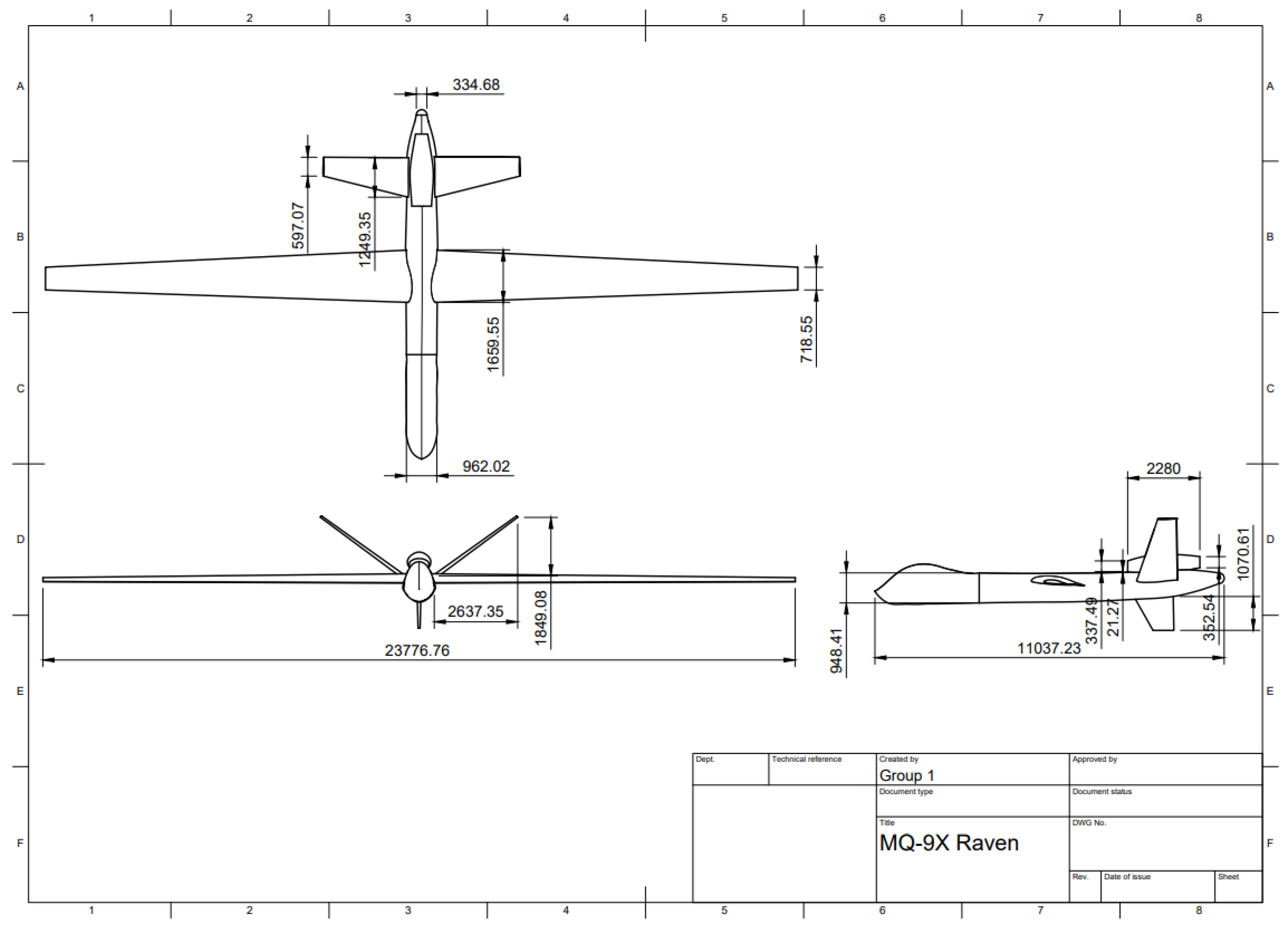
Table A1.
Operational characteristics summary: MQ-9A Reaper versus MQ-9X Raven
| Characteristic | MQ-9A Reaper (Current) | MQ-9X Raven (Proposed) |
|---|---|---|
| Role/Mission Focus | Multi-mission ISTAR and Strike | Persistent, Long-Range, High-Altitude ISR and Long-Range Strike |
| Endurance (Maximum) | 27 hours (Claimed) | 13 hours (Mission Time + Transit) |
| Ceiling (Claimed/Operating) | 50,000 ft (Claimed) | 50,000 ft (Operating Altitude in Redefined Mission Profile) |
| Cruise Speed (Redefined) | N/A (Max Speed 240 kts) | 130 KIAS (300 KTAS) |
| Operational Radius (Redefined) | N/A | 1,800 nm (Based on 6-hour cruise at 300 KTAS) |
| MTOW | 4,672 kg | 6,123kg (Increased fuel capacity, JSM integration, larger wings, and new engine.) |
| Powerplant | Honeywell TPE331-10GD Turboprop | Williams FJ-44A |
| Wingspan | Standard MQ-9A | 79 ft (Increased) |
| Airfoil | Standard MQ-9A | LRN1015 |
| Primary Munitions | Standard (Implied, not detailed) | Joint Strike Missile (JSM) |
| Cruise Profile | Primarily medium altitude, slow speed | Persistent high-altitude (50,000 ft), higher airspeed |
| Climb Rate (Requirement) | N/A (Reference: ≤2000 ft/min) | >2000 ft/min |
| Strategic Goal | Versatile, but less capable in peer environments | Deterrent, project power, support allied operations in contested airspace |
Appendix B. Constant Energy Height Map
Figure A2.
Drag Polar
Appendix C. Specific Excess Power
Figure A3.
Drag Polar
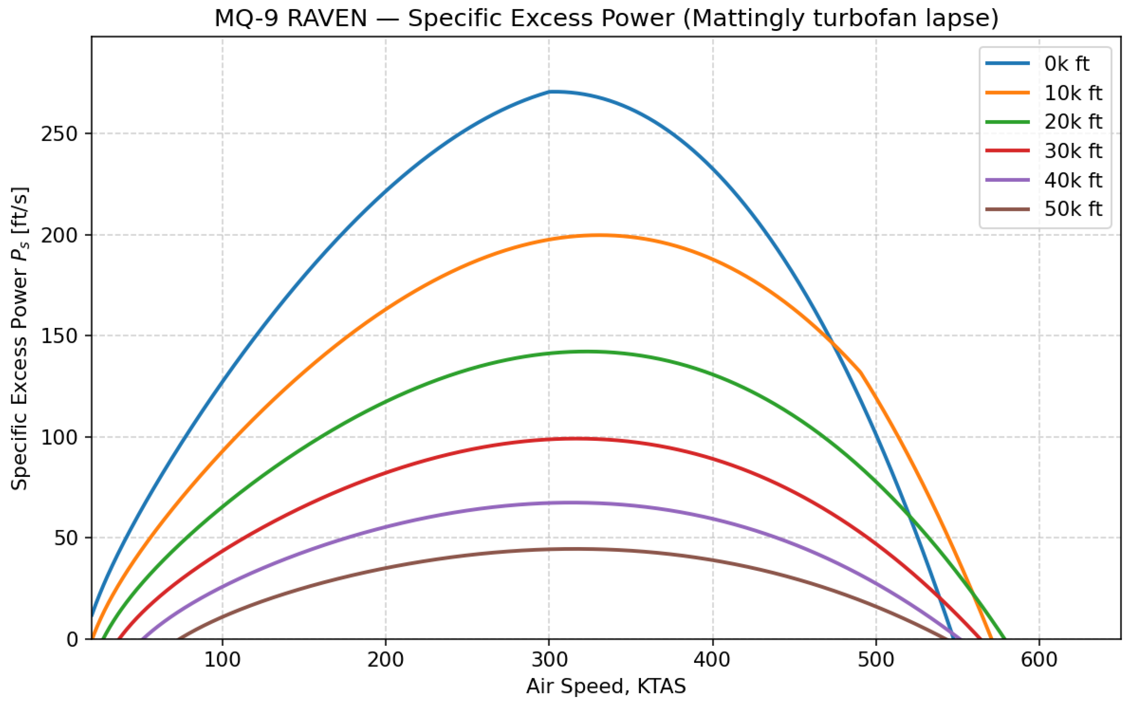
Figure A4.
Drag Polar
Appendix D. Thrust Analysis
Figure A5.
Thrust Available vs Thrust Required.
Appendix E. CoG envelope
Figure A6.
Centre-of-gravity (CG) envelope for the Raven, showing the forward and aft limits derived from nose landing gear (NLG) and main landing gear (MLG) structural constraints. The shaded region represents the permissible CG range across the aircraft weight envelope.
Figure A6.
Centre-of-gravity (CG) envelope for the Raven, showing the forward and aft limits derived from nose landing gear (NLG) and main landing gear (MLG) structural constraints. The shaded region represents the permissible CG range across the aircraft weight envelope.
Appendix F. Weapon Integration Test Matrix
Table A2.
Test Campaign Matrix
| Test ID | Phase | Test Case | Speed | Altitude | Configuration |
|---|---|---|---|---|---|
| P1-CAD-001 | Phase 1 | MOI extraction & CAD verification | N/A | N/A | N/A |
| P1-CFD-001 | Phase 1 | CFD - Isolated JSM across AoA/Mach | 0.1–0.8 Mach | Sea level to 45,000 ft | Isolated store |
| P1-CFD-002 | Phase 1 | CFD - Store attached to pylon on wing | 0.1–0.8 Mach | Sea level to 45,000 ft | Store on pylon, multiple stations |
| P1-AERO-001 | Phase 1 | DATCOM/AVL coefficient derivation | 0–0.9 Mach | Sea level to 45,000 ft | Store & aircraft models |
| P1-FEM-001 | Phase 1 | FEM structural analysis of pylon & wing | N/A | N/A | Static & dynamic loads |
| P1-FLUT-001 | Phase 1 | Aeroelastic / flutter analysis with store | 0–0.9 Mach | Sea level to 45,000 ft | Full aircraft with store |
| P1-AST-001 | Phase 1 | ASTERIX separation modelling - baseline | 0.1–0.6 Mach | Sea level to 45,000 ft | Clean & loaded |
| P2-WT-001 | Phase 2 | Wind tunnel - isolated store balance tests | Scaled Mach ranges | N/A | Scale model |
| P2-WT-002 | Phase 2 | Wind tunnel - store on semi-span model | Scaled Mach ranges | N/A | Semi-span wing+pylon |
| P3-GND-001 | Phase 3 | Pylon static proof load & fitting checks | N/A | N/A | Static ground |
| P3-ENV-001 | Phase 3 | EMC/EMI & DO-160G environmental tests (avionics & weapon) | N/A | N/A | Ground lab |
| P4-CAP-001 | Phase 4 | Captive carry - low speed envelope expansion | Up to 0.3 Mach | Up to 10,000 ft | Clean |
| P4-CAP-002 | Phase 4 | Captive carry - high altitude/high speed | Up to 0.8 Mach | Up to 40,000 ft | Clean & transit |
| P5-REL-001 | Phase 5 | Instrumented release - benign conditions (low speed) | 0.1–0.2 Mach | 10,000–20,000 ft | Clean |
| P5-REL-002 | Phase 5 | Instrumented release - expanded envelope | 0.3–0.8 Mach | 5,000–45,000 ft | Various flap/trim |
| P6-LVE-001 | Phase 6 | Captive live-weapons ferry (safe-to-arm checks) | Transit speeds | Operational cruise | Clean |
| P7-LIVE-001 | Phase 7 | Live JSM release & mission validation | Operational release speeds | Operational release altitude 45,000 ft | Mission representative |
| CERT-001 | Phase 8 | Certification dossier compilation & submission | N/A | N/A | N/A |
References
- General Atomics Aeronautical Systems, Inc.. MQ-9A Remotely Piloted Aircraft, n.d. Accessed: 2025-06-02.
- Zountouridou, E.; Kiokes, G.; Dimeas, A.; Prousalidis, J.; Hatziargyriou, N. A Guide to Unmanned Aerial Vehicles Performance Analysis—The MQ-9 Unmanned Air Vehicle Case Study. The Journal of Engineering 2023, 2023, e12270. [CrossRef]
- Adeleke, O.A.; Abbe, G.E.; Jemitola, P.O.; Thomas, S. Design of the Wing of a Medium Altitude Long Endurance UAV. International Journal of Engineering and Manufacturing (IJEM) 2022. [CrossRef]
- Gudmundsson, S. General Aviation Aircraft Design: Applied Methods and Procedures; Butterworth–Heinemann, 2013.
- Smithsonian Institution. Williams FJ44 Turbofan Engine. Smithsonian Institution, 2025.
- Gudmundsson, S. General Aviation Aircraft Design: Applied Methods and Procedures (2nd ed.); Elsevier, 2022. Retrieved from Knovel.
- Zountouridou, E.; Kiokes, G.; Dimeas, A.; Prousalidis, J.; Hatziargyriou, N. A Guide to Unmanned Aerial Vehicles Performance Analysis—The MQ-9 Unmanned Air Vehicle Case Study. The Journal of Engineering 2023, 2023, e12270. [CrossRef]
- JD Tech Sales. Hydraulic actuator replacement using electromechanical technology, n.d. White paper. Retrieved July 29, 2025, from JD Tech Sales website.
- Torenbeek, E. Advanced Aircraft Design: Conceptual Design, Analysis and Optimization of Subsonic Civil Airplanes; John Wiley & Sons: Chichester, UK, 2013.
- Ostermann, M.; Schodl, J.; Lieberzeit, P.A.; Bilotto, P.; Valtiner, M. Lightning Strike Protection: Current Challenges and Future Possibilities. Materials 2023, 16, 1743. [CrossRef]
- Unknown author. Valuation Techniques for Commercial Aircraft Program Design; Massachusetts Institute of Technology, n.d. Unpublished doctoral dissertation; available from DSpace@MIT.
- Mach Tres. General Atomics MQ-1 Predator / MQ-9 Reaper. https://www.machtres.com/lang1/predator.html, n.d. Accessed: 22 May 2025.
- Patterson, M.D.; Arena, M.V. UAV Employment in Korea: A Concept for the Future. Technical Report ADA427459, RAND Corporation, Santa Monica, CA, 2004. Accessed: 22 May 2025.
- Gudmundsson, S. General Aviation Aircraft Design: Applied Methods and Procedures; Butterworth–Heinemann: Oxford, 2013.
- Zountouridou, E.; Kiokes, G.; Dimeas, A.; Prousalidis, J.; Hatziargyriou, N. A Guide to Unmanned Aerial Vehicles Performance Analysis—The MQ-9 Unmanned Air Vehicle Case Study. The Journal of Engineering 2023. [CrossRef]
- Manaf, M.Z.A.; Mat, S.; Mansor, S.; Nasir, M.N.; Lazim, T.M.; Ali, W.; Othman, N. Influences of External Store on Aerodynamic Performance of UTM-LST Generic Light Aircraft Model. Journal of Advanced Research in Fluid Mechanics and Thermal Sciences 2017.
- Hicks, R.M.; Cliff, S.E. An Evaluation of Three Two-Dimensional Computational Fluid Dynamics Codes Including Low Reynolds Numbers and Transonic Mach Numbers. Technical report, NASA, 1991.
- van Kuik, G. The Fluid Dynamic Basis for Actuator Disc and Rotor Theories: Revised Second Edition; TU Delft Open Publishing, 2022.
- European Union Aviation Safety Agency (EASA). Type-Certification Data Sheet for FJ44/FJ33 Series Engines, 2021.
- NETAVIO. Williams FJ44-4A Full Authority Digital Engine Control (FADEC) Controlled Turbofan Engines. X-Plane.org Forum, 2021. June 2021.
- International Standard Atmosphere (ISA). Performance of the Jet Transport Airplane: Analysis Methods, Flight Operations and Regulations, 2017. pp. 583–590.
- Williams International. Home Page – Williams International, 2025.
- Schmidle, N. The Unblinking Stare – The Drone War in Pakistan. The New Yorker 2014.
- Huff, D.L. Noise Reduction Technologies for Turbofan Engines. Technical report, NASA Glenn Research Center, 2007.
- Austin, R. Unmanned Aircraft Systems: UAV Design, Development and Deployment; John Wiley & Sons, 2010.
- NASA Glenn Research Center. Noise-Reduction Benefits for Over-the-Wing Mounted Engines. Technical report, NASA, 1999.
- Williams International. FJ44-4A-QPM Engine Features for Pilatus PC-24. Flying Magazine 2014.
- Sutliff, D.L.; Elliott, D.M.; Jones, M.G.; Hartley, T.C. Attenuation of FJ44 Turbofan Engine Noise with a Foam-Metal Liner Installed Over-the-Rotor. Technical report, NASA Glenn Research Center, 2009.
- Joint Air Power Competence Centre. The Vulnerabilities of Unmanned Aircraft System Components; In Countering Unmanned Aircraft Systems (C-UAS), Chapter 4, Kalkar, Germany, 2020.
- General Atomics Aeronautical Systems. MQ-20 Avenger (Predator C) Data Sheet, 2018.
- Zhou, Z.; Huang, J. Study of the Radar Cross-Section of Turbofan Engine with Biaxial Multirotor Based on Dynamic Scattering Method. Energies 2020. [CrossRef]
- Dunstone, P.; Medway, L.; O’Neill, N.; Tenhave, J.; Tenneti, R. Critical Analysis of the MQ-9A Reaper and Proposed Modifications. Technical report, University of New South Wales at the Australian Defence Force Academy, 2025.
- Nelson, R.C. Flight Stability and Automatic Control, 2 ed.; McGraw-Hill, 2007.
- Stengel, R.F. Flight Dynamics; Princeton University Press, 2005.
- YouTube video creator. Dynamic longitudinal stability. YouTube video, n.d. Retrieved July 29, 2025.
- Cook, M.V. Chapter 6 – Longitudinal Dynamics. In Flight Dynamics Principles, 3 ed.; Butterworth-Heinemann, 2013; pp. 147–181. [CrossRef]
- Stability and Control. Volume I: Stability and Control Flight Test Techniques. Technical report, Air Force Flight Test Center, Edwards Air Force Base, California, 1974. Technical Report, Volume I.
- Budziak, K., .S. Aerodynamic Analysis with Athena Vortex Lattice (AVL), n.d.
- Litherland, B. Modeling Best-Practices for VSPAERO, 2021. 2021 OpenVSP Workshop, Virtual Broadcast.
- Anafi, S.O.; Najam, T.; Pampori, A.M.; Moses, J.K. Enhanced Stability and Aerodynamic Performance of the Skywalker X8 UAV using a V-Tail: A Comprehensive Modeling and Analysis Using OpenVSP Software. In Proceedings of the AIAA 2025-0145: Session: Modeling and Simulation of UAS/UAM/AAM Vehicle Dynamics, Systems, and Environments I, 2025.
- Kish, B. Lateral/Directional Dynamic Stability [YouTube video]. https://www.youtube.com/watch?v=wfFS6Ned1K4, 2020. Accessed: 2025-11-03.
- Research, L. X-Plane 11 Digital Download (Desktop Edition). Digital download for Windows, macOS and Linux, 2023. Accessed: 2025-11-03.
- Drela, M.; Youngren, H. Athena Vortex Lattice (AVL) - Aerodynamic and Flight-Dynamic Analysis Program, 2022. Accessed: 2025-11-03.
- Kongsberg Defence & Aerospace. Joint Strike Missile (JSM), n.d. Retrieved July 29, 2025, from Kongsberg website.
- Zen13. Naval Strike Missile (Thing: 6891849). https://www.thingiverse.com/thing:6891849, 2024. 3D model.
- Force, U.A. RQ-4 Global Hawk, 2014.
- Daugherty, J.C. Ames Unitary Plan Wind Tunnel Blockage Recommendations, 1984. Accessed: 2025-10-08.
- Barlow, J.B.; Rae, W.H.J.; Pope, A. Low-Speed Wind Tunnel Testing, 3 ed.; John Wiley & Sons Inc., 1999.
- Winslow, J.; Otsuka, H.; Govindarajan, B.; Chopra, I. Basic Understanding of Airfoil Characteristics at Low Reynolds Numbers. Journal of Aircraft 2018, pp. 1067–1080. [CrossRef]
- Rona, A., .S.H. Boundary layer trips for low Reynolds number wind tunnel tests. In Proceedings of the 48th AIAA Aerospace Sciences Meeting, 2010, January, pp. 399+.
- Traub, L.W. Scale Effects in Wind Tunnel Testing: Extrapolation of the Drag Coefficient. Journal of Aircraft 2024, pp. 1482–1489. [CrossRef]
| 1 | Data used was Re= and Re=
|
Figure 1.
Redefined Raven mission profile
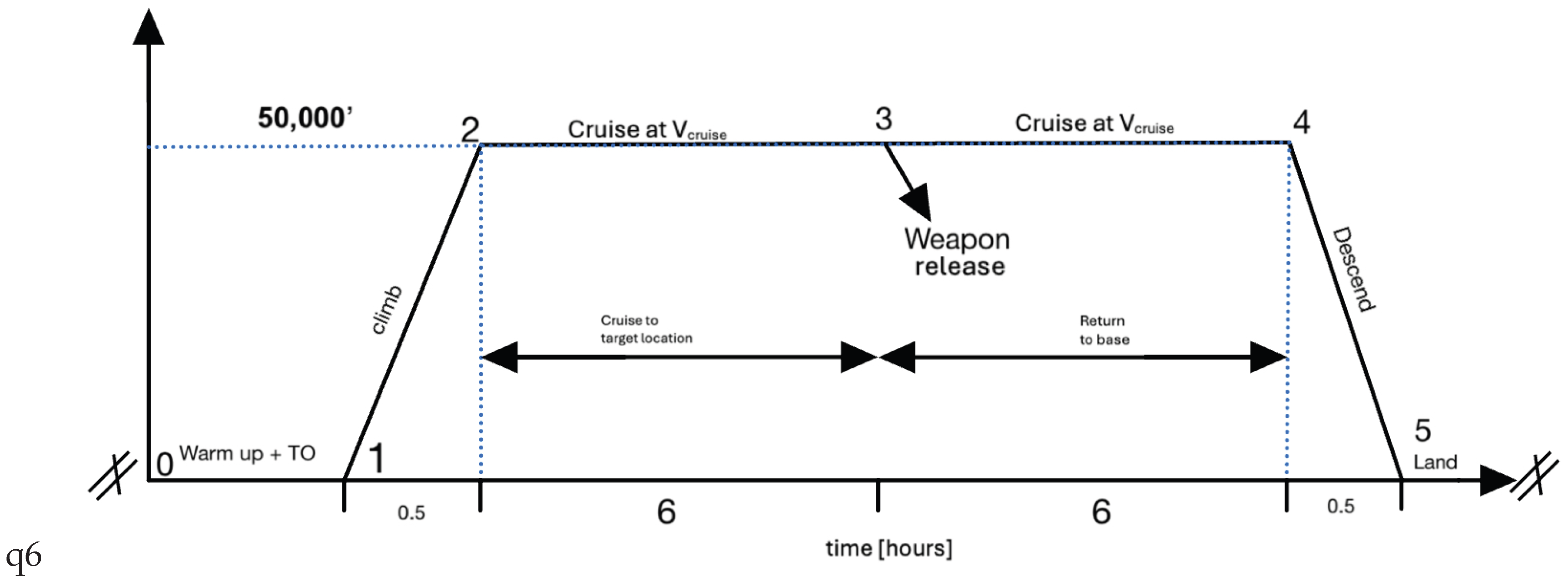
Figure 2.
Surface pressure plot at for , , , and CG located aft of the nose
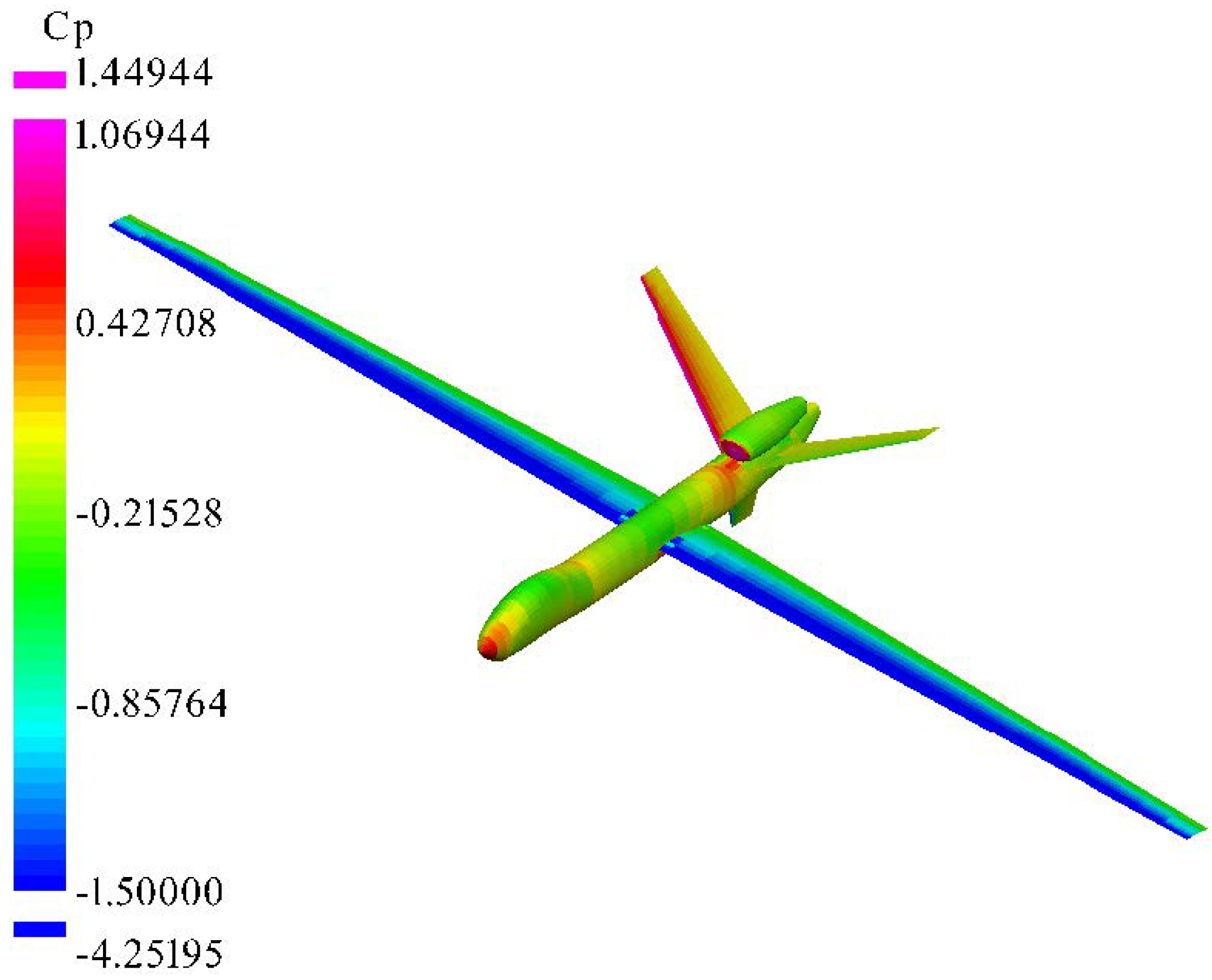
Figure 3.
-Sweep for , , , and CG located aft of the nose
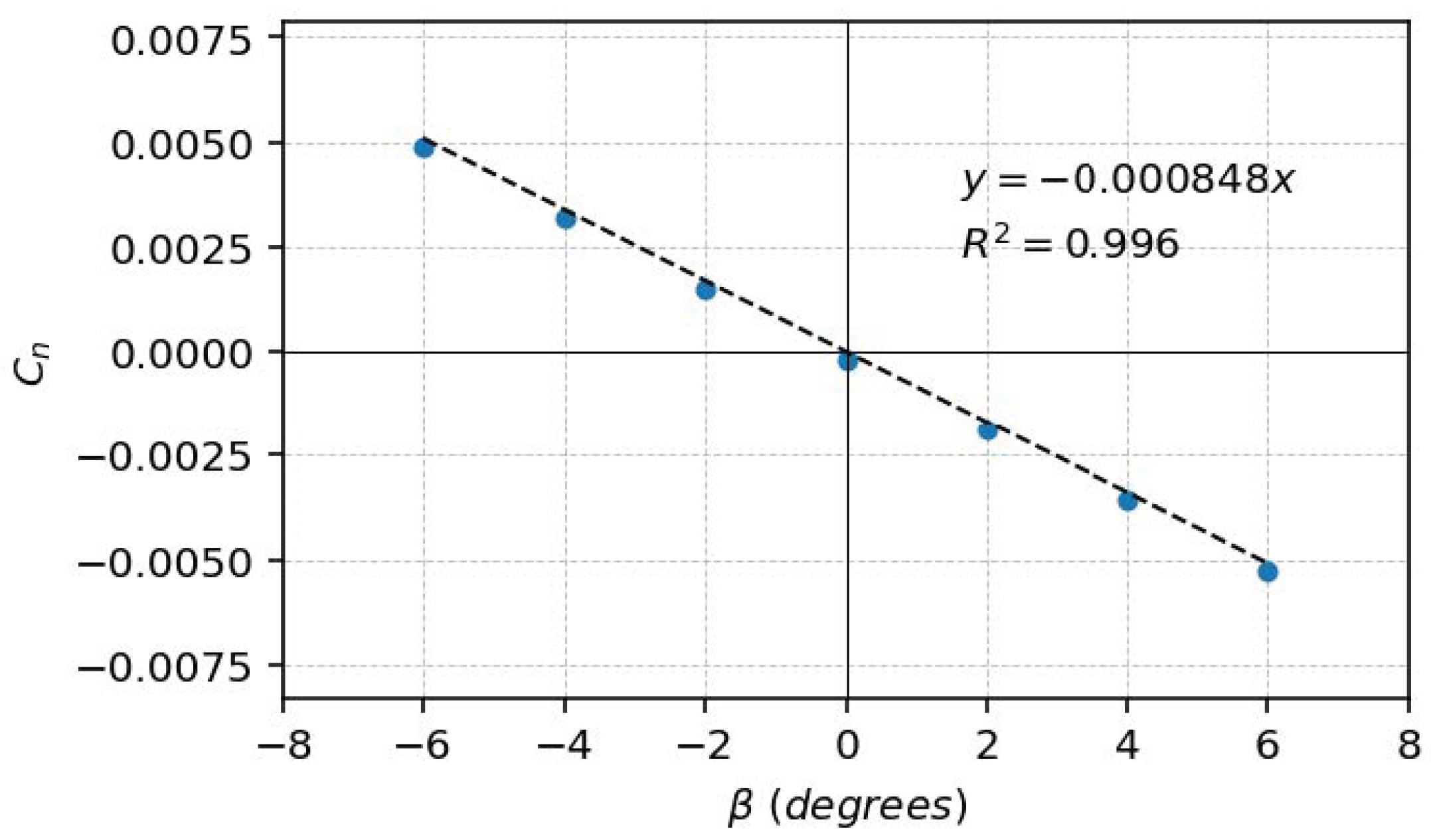
Figure 4.
Three Raven tail variants for further stability analysis
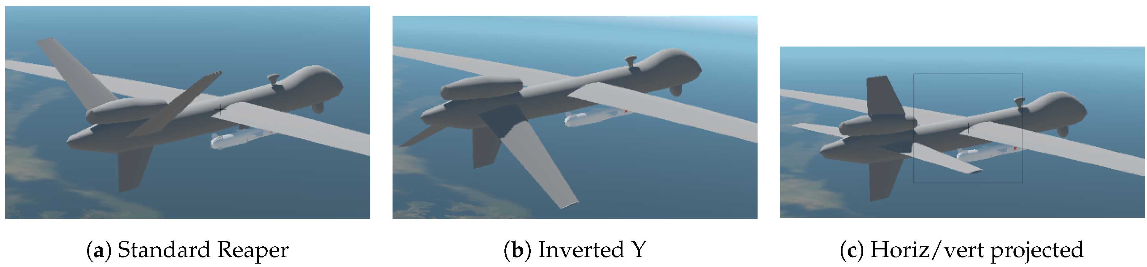
Figure 5.
Static stability of 3 tail variants
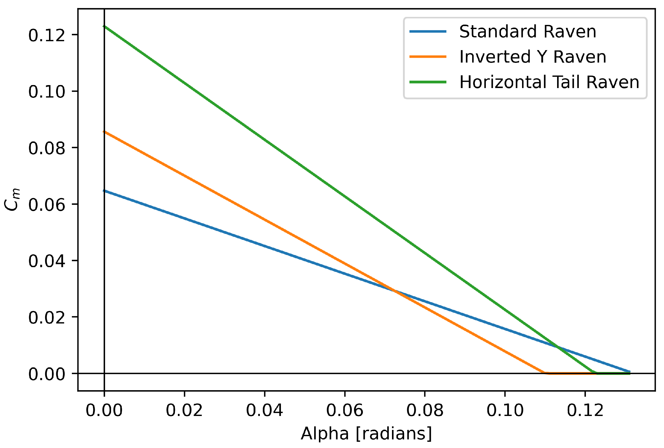
Figure 6.
Example AVL Python Script for the Dutch Roll Mode with the Raven Y-Tail
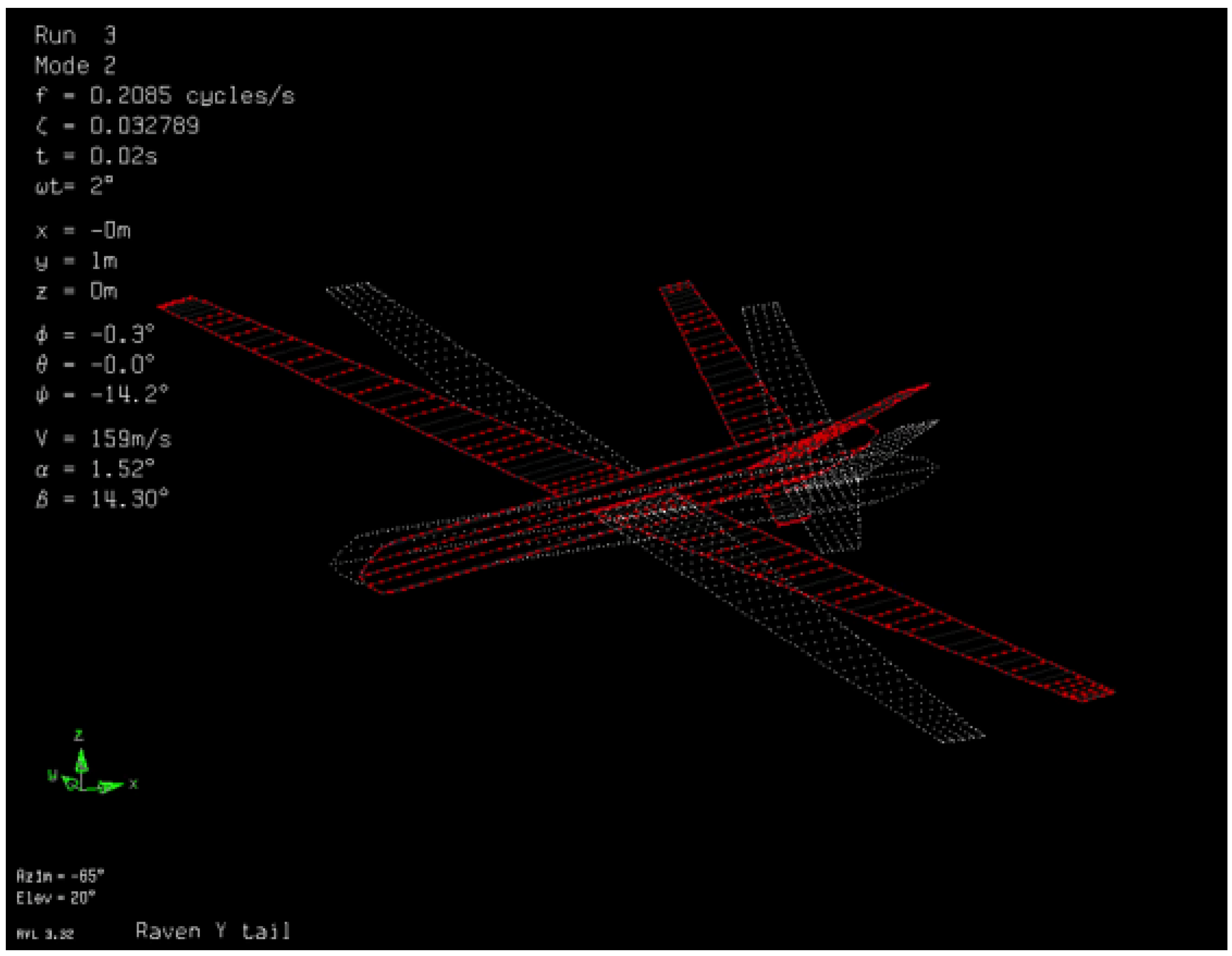
Figure 7.
Comparison of lift slope results.
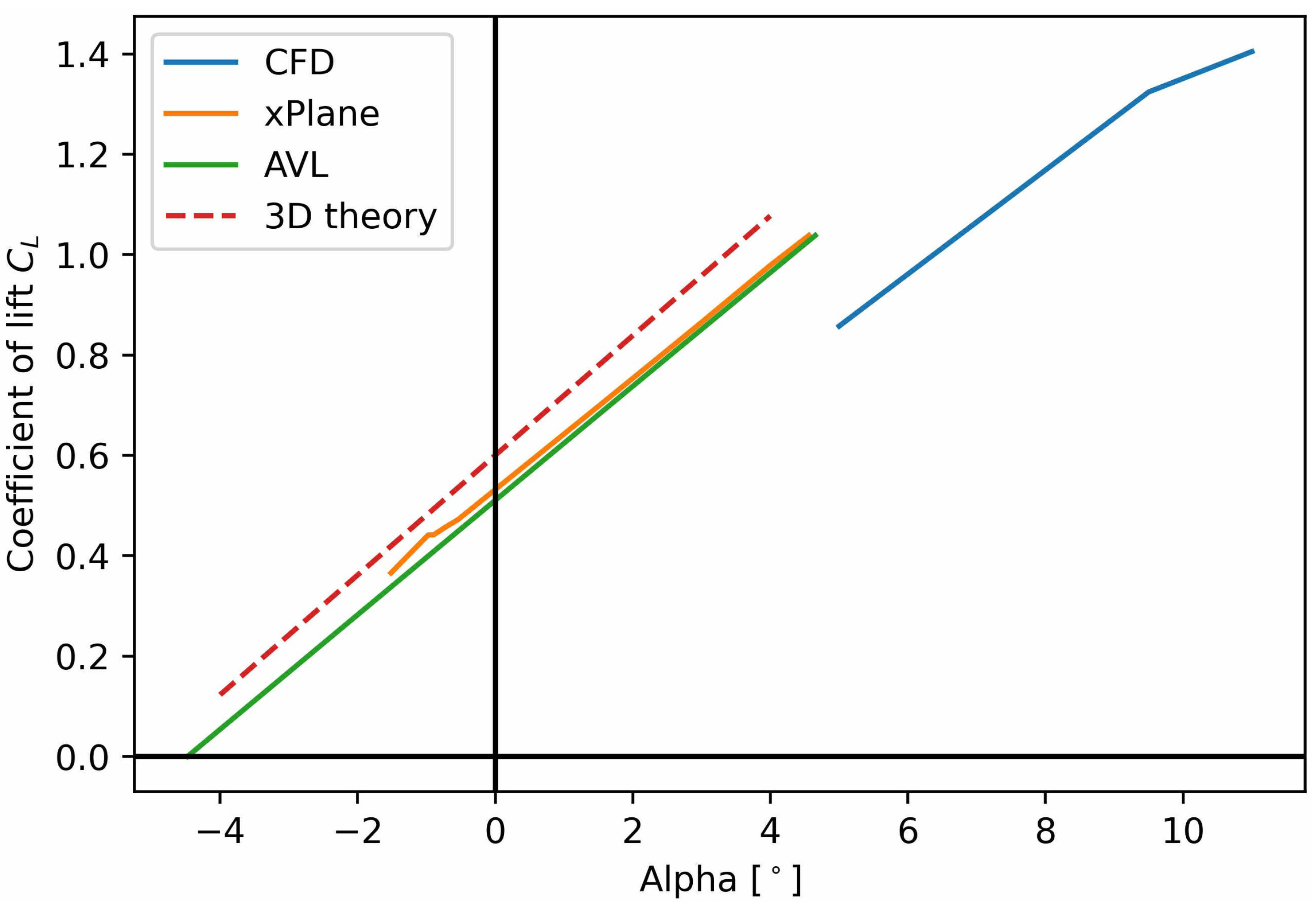
Figure 8.
Drag Coefficient versus Angle of Attack (AoA) (Notes: error bars: 95% confidence intervals, Wind Tunnel results in blue)
Figure 8.
Drag Coefficient versus Angle of Attack (AoA) (Notes: error bars: 95% confidence intervals, Wind Tunnel results in blue)
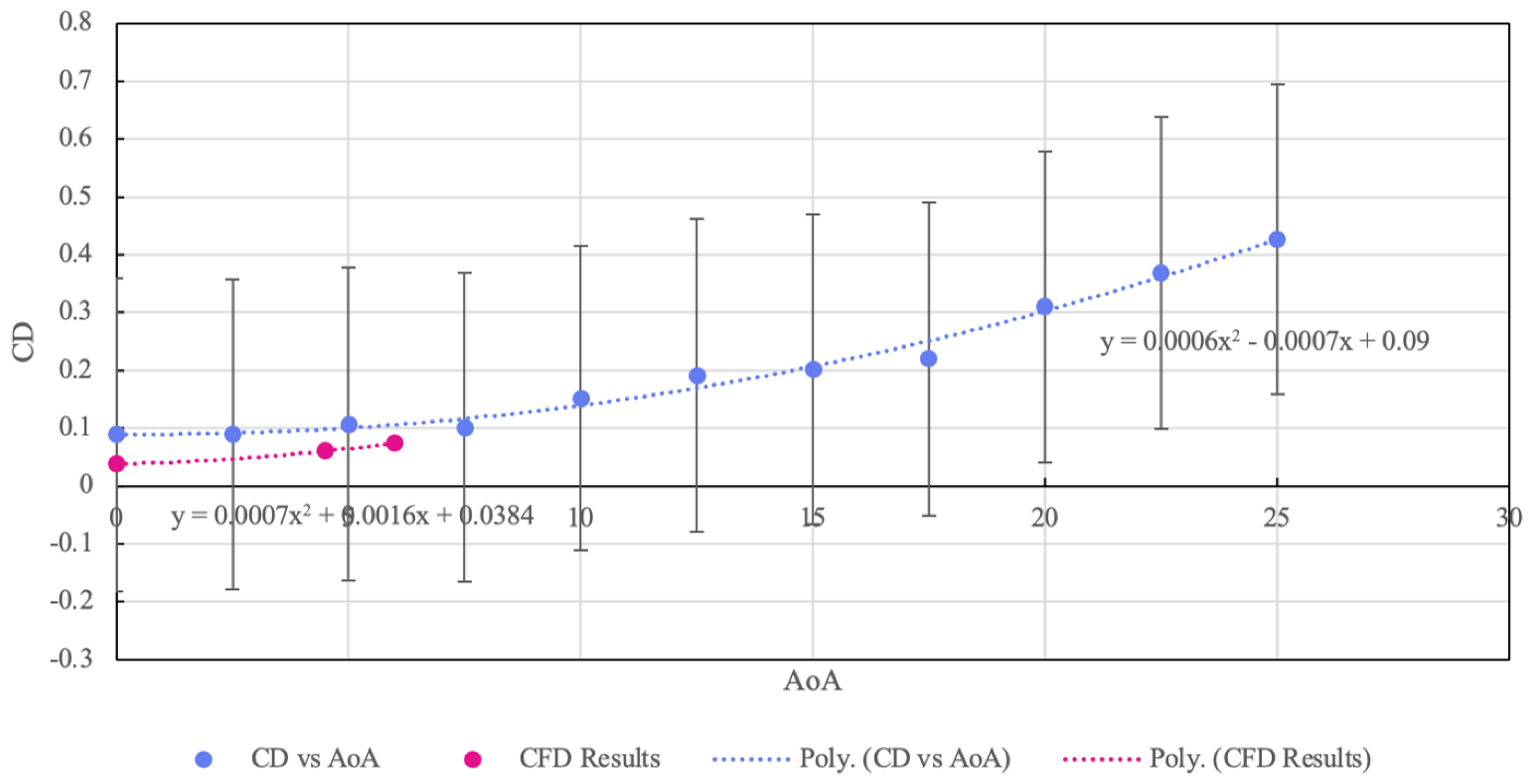
Figure 9.
Velocity contour on aircraft’s plane of symmetry.
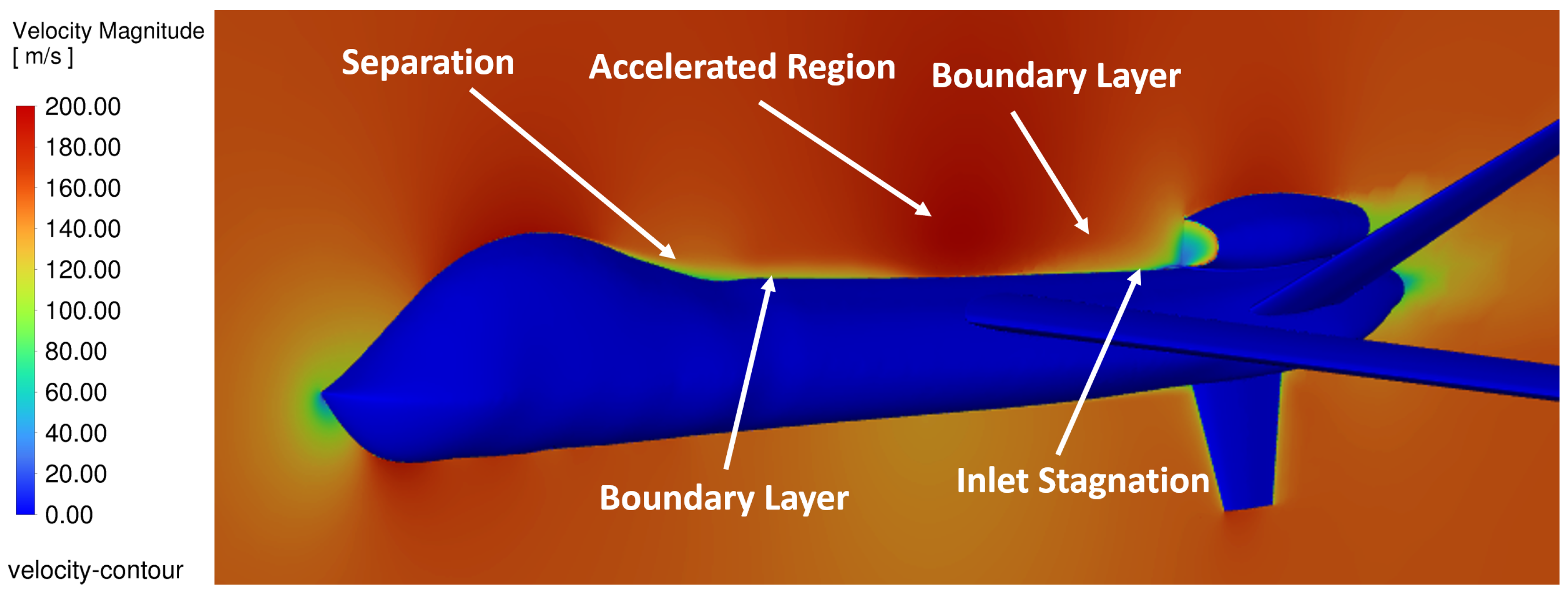
Figure 10.
Streamlines around the fuselage indicating changes to velocity magnitudes.
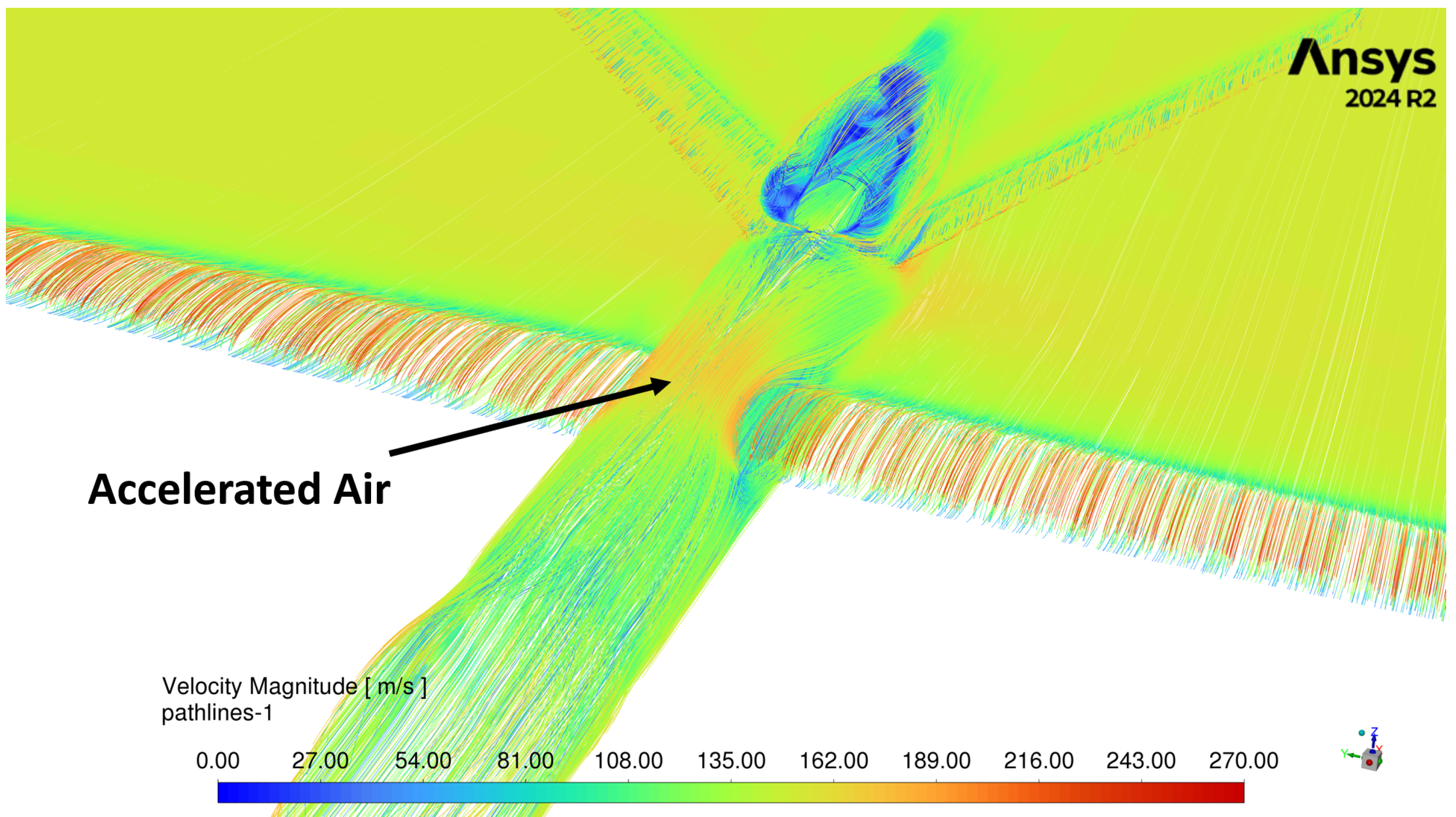
Figure 11.
Velocity contour on aircraft’s plane of symmetry at the engine inlet.
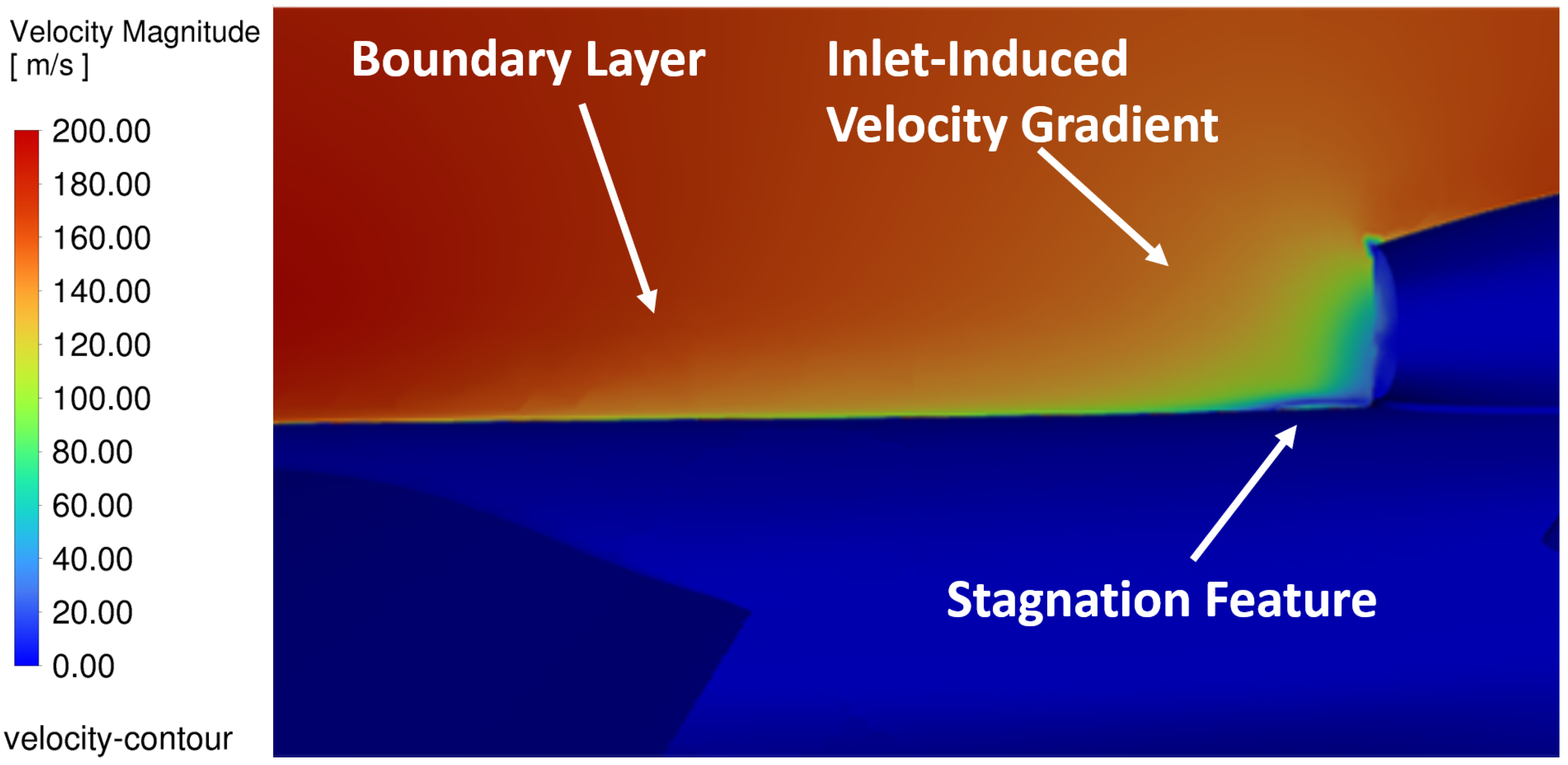
Figure 12.
Lambda2-Criterion iso-surface of engine section, with upper limit set to -100 (Note an ANSYS method number 12.1.8.1.2.1.)
Figure 12.
Lambda2-Criterion iso-surface of engine section, with upper limit set to -100 (Note an ANSYS method number 12.1.8.1.2.1.)
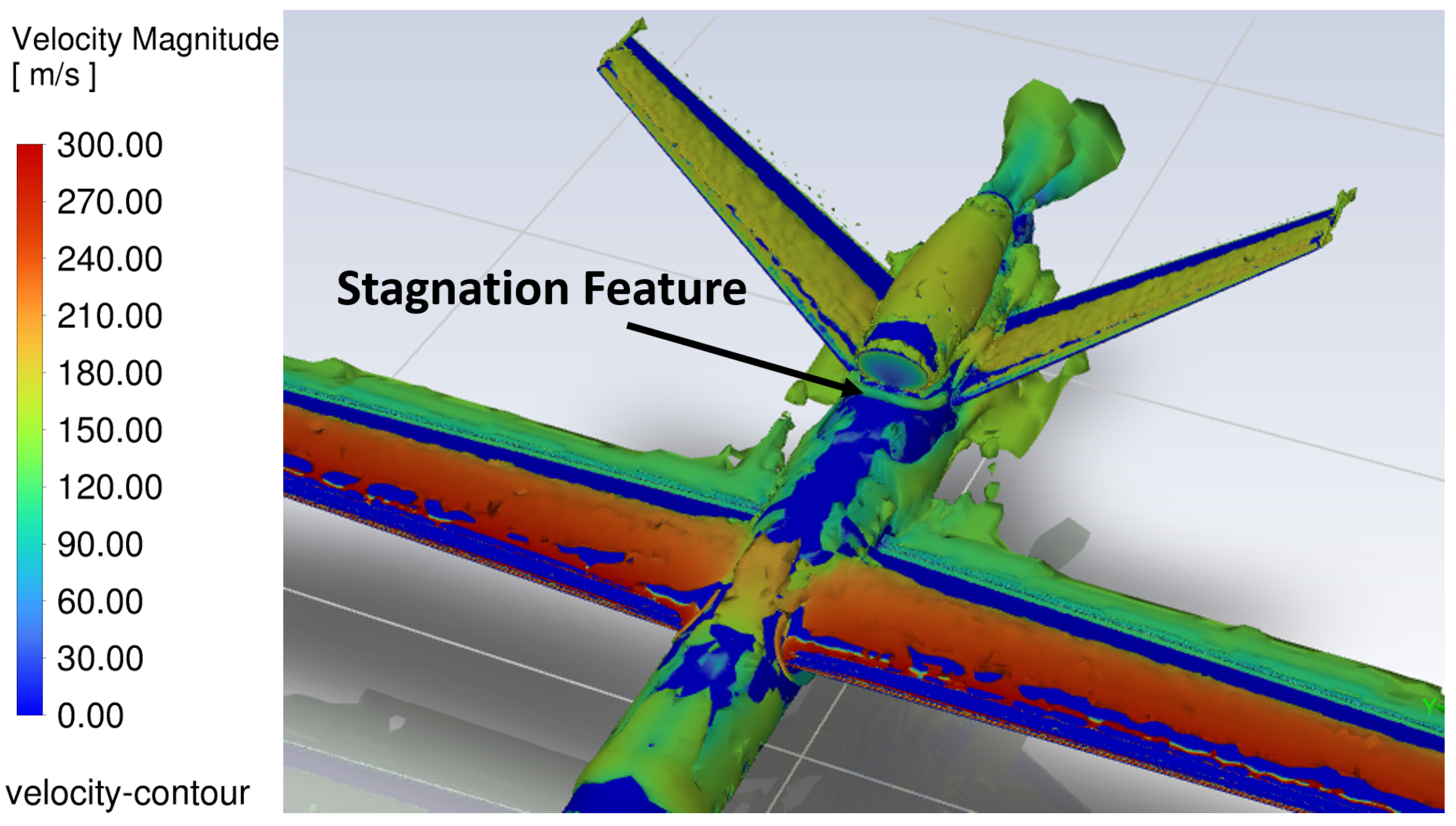
Figure 13.
Image of RQ-4 Globalhawk showing engine inlet clearance and overhang for delayed stagnation [46].
Figure 13.
Image of RQ-4 Globalhawk showing engine inlet clearance and overhang for delayed stagnation [46].
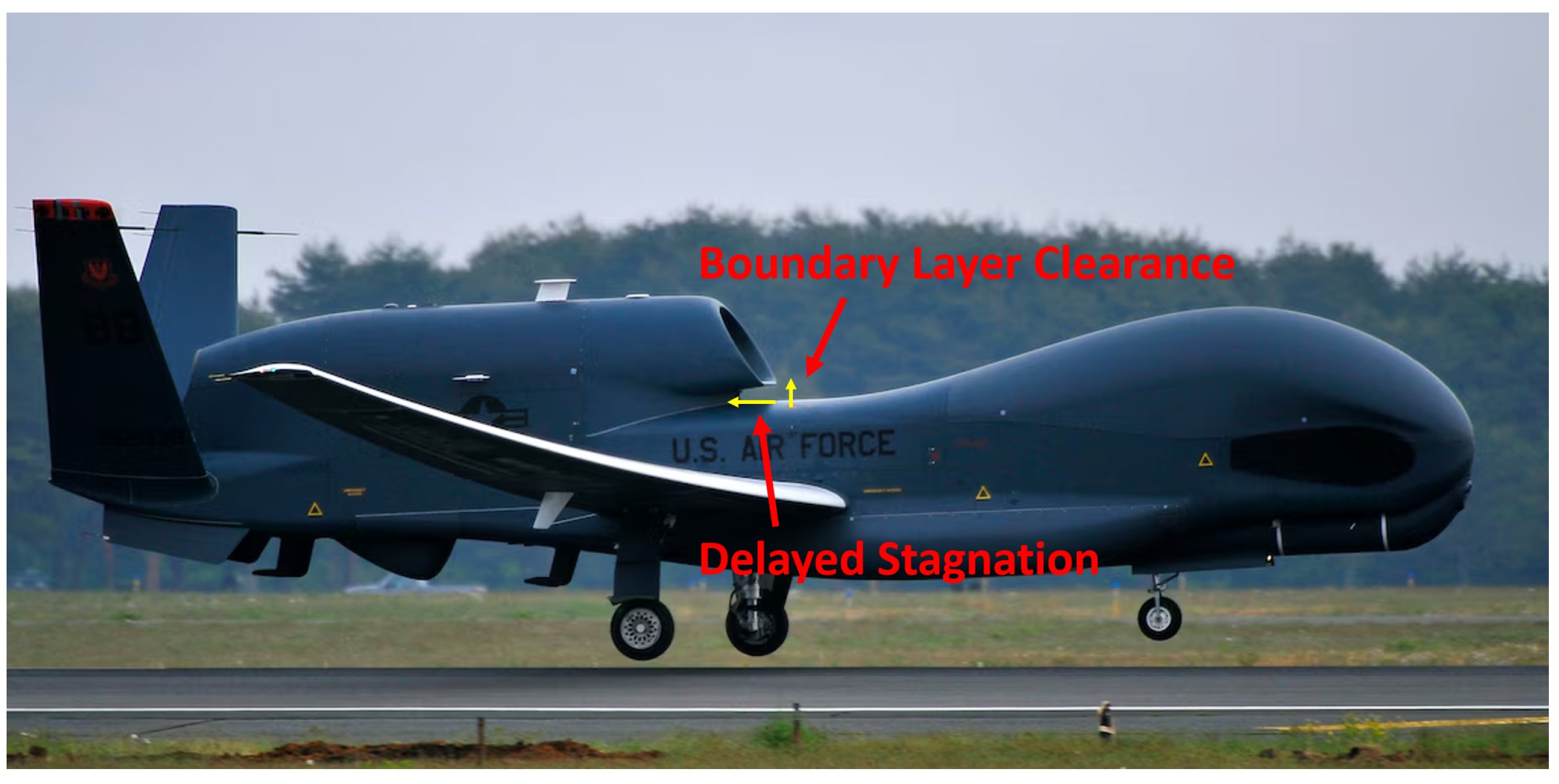
Figure 14.
Manufacture of Wind Tunnel Model
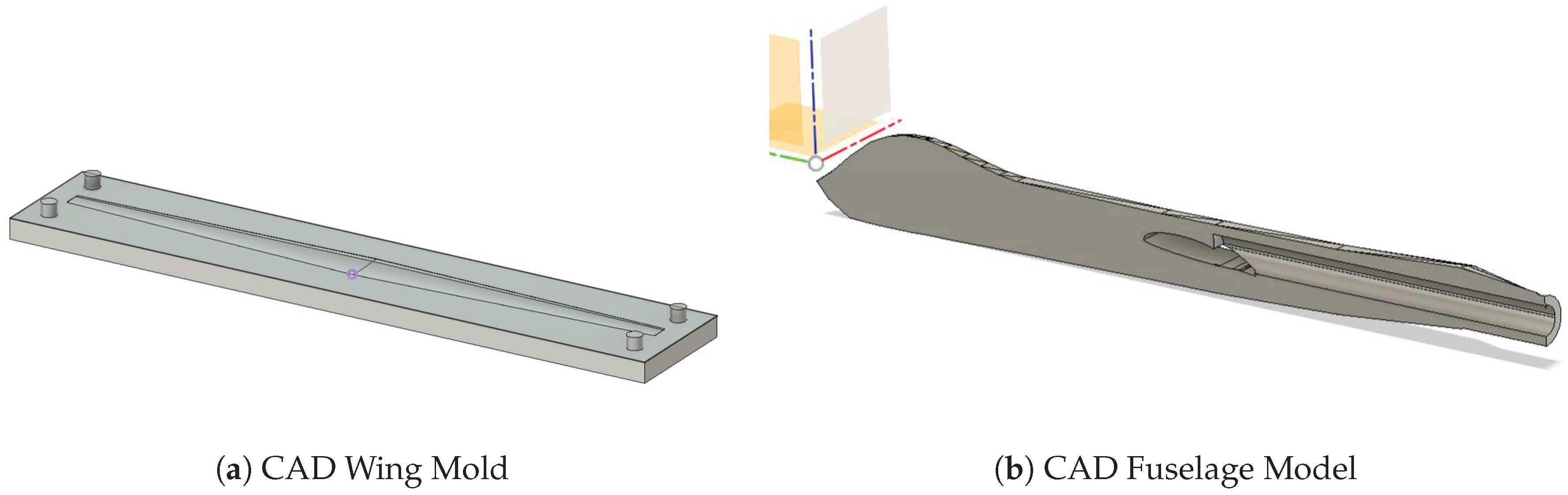
Figure 15.
Wind Tunnel Model Mounted
Figure 16.
Lift Coefficient versus Angle of Attack (AoA) (Note: error bars are 95% confidence intervals and Pink is the Wind Tunnel results)
Figure 16.
Lift Coefficient versus Angle of Attack (AoA) (Note: error bars are 95% confidence intervals and Pink is the Wind Tunnel results)
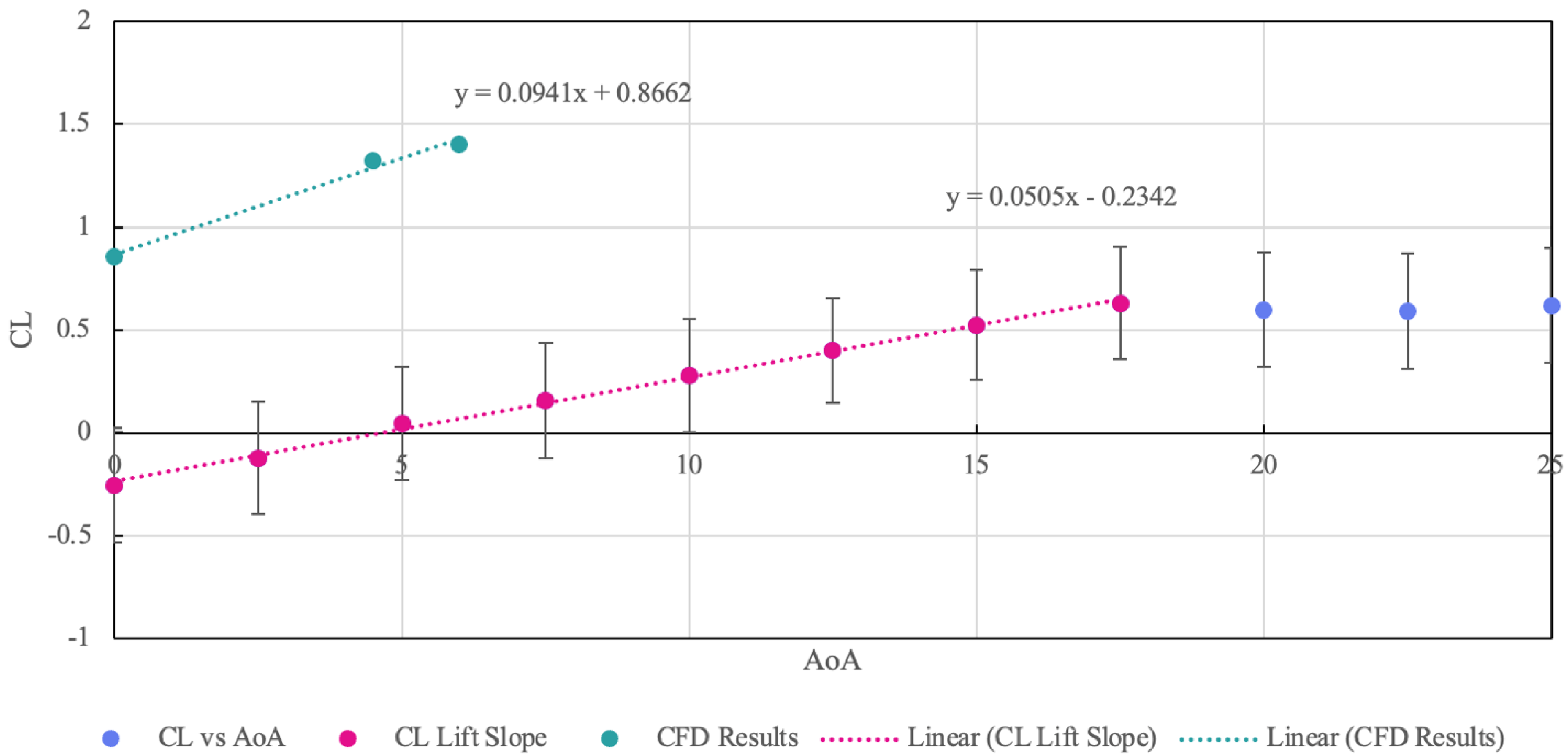
Table 3.
Dihedral effect for the MQ-9X Raven.
| Component | Parameter / Description | (rad−1) |
|---|---|---|
| Wing | Main planar surface, dihedral | 0 |
| V-tail | dihedral effect, | |
| Ventral fin | Secondary coupling contribution | |
| Total (aircraft) |
Table 4.
Simulation Dynamic Stability Values for 3 Tail Variants
| Phugoid | Short Period | Dutch Roll | Spiral | ||||
|---|---|---|---|---|---|---|---|
| T [s] | |||||||
| Standard | 0.0360 | 0.110 | 0.993 | 0.662 | 0.0906 | 1.66 | 95.5 |
| Inverted Y | 0.0287 | 0.107 | 0.913 | 0.657 | 0.0837 | 1.23 | 74.6 |
| Horiz/Vert | 0.0302 | 0.110 | 0.960 | 0.798 | 0.0763 | 1.31 | 104 |
Table 5.
Simulation Dynamic Stability Levels
| Phugoid | Short Period | Dutch Roll | Spiral | |
|---|---|---|---|---|
| Standard | Level 2 | Level 1 | Level 1 | Level 1 |
| Inverted Y | Level 2 | Level 1 | Level 2 | Level 1 |
| Horiz/Vert | Level 2 | Level 1 | Level 2 | Level 1 |
Table 6.
AVL capabilities used for JSM analysis.
| Capability | Description |
|---|---|
| Static stability and trim analysis | Prediction of aerodynamic forces and moments and determination of trim points for given flight conditions. |
| Dynamic stability (eigenmode/root-locus) | Linearised small-perturbation eigenvalue analysis to obtain short period, phugoid, Dutch roll and other modes. |
| Control surface and mass property modelling | Inclusion of control surface deflections, CG location, and approximate moments of inertia (MOI) to assess control authority and stability derivatives. |
Table 7.
AVL analysis workflow implemented for the JSM.
| Step | Action | Notes |
|---|---|---|
| 1 | Acquire a 3D STL model of the JSM. | Reference: [45] |
| 2 | Import and scale geometry in Fusion 360 to obtain reference dimensions (span, area, MAC). | Geometry scaling used to define aerodynamic reference quantities. |
| 3 | Estimate mass properties (CG, MOI) using volume and density averaging. | Approximations used for initial MOI inputs to AVL. |
| 4 | Construct the aerodynamic model in AVL, including lifting and control surfaces. | Symmetric NACA-0012 was assumed for lifting sections. |
| 5 | Execute static and dynamic stability analyses across multiple flight conditions. | Static sweeps and eigenmode analysis performed. |
Table 8.
Key static stability results from AVL (-sweep).
| Parameter | Value | Comment |
|---|---|---|
| Neutral point, | Non-dimensionalised about reference chord | |
| Static margin | – | Small static margin; trade-off manoeuvrability vs stability |
| Negative slope indicates static stability in pitch |
Table 9.
Trim feasibility across representative operating conditions.
| Condition | Altitude | Speed | Trim Achieved? | (deg) |
|---|---|---|---|---|
| MQ-9 cruise reference | 50,000 ft | 300 KTAS | No | >150 (no feasible trim) |
| MQ-9 cruise + JSM speed | 50,000 ft | Mach 0.9 | Yes (but impractical) | (high drag) |
| JSM nominal cruise (sea level) | Sea level | Mach 0.9 | Yes | (efficient sea-skimming trim) |
Table 10.
Dynamic stability eigenmodes at trimmed sea-level condition (AVL eigenvalue analysis).
| Mode | Frequency (cycles/s) | Damping ratio | Stability / Comment |
|---|---|---|---|
| Short Period | Stable (adequate damping in pitch) | ||
| Phugoid | Stable (slow lightly-damped phugoid) | ||
| Dutch Roll | Lightly unstable / nearly neutral (yaw damping augmentation likely required) |
Disclaimer/Publisher’s Note: The statements, opinions and data contained in all publications are solely those of the individual author(s) and contributor(s) and not of MDPI and/or the editor(s). MDPI and/or the editor(s) disclaim responsibility for any injury to people or property resulting from any ideas, methods, instructions or products referred to in the content. |
© 2025 by the authors. Licensee MDPI, Basel, Switzerland. This article is an open access article distributed under the terms and conditions of the Creative Commons Attribution (CC BY) license (http://creativecommons.org/licenses/by/4.0/).
Copyright: This open access article is published under a Creative Commons CC BY 4.0 license, which permit the free download, distribution, and reuse, provided that the author and preprint are cited in any reuse.


