
Submitted:
14 November 2025
Posted:
17 November 2025
You are already at the latest version
Abstract
In this study, a traffic flow analysis was conducted using a multi-agent simulation to evaluate the effect of reducing CO2 emissions through the penetration of connected autonomous vehicles (CAVs) equipped with vehicle-to-vehicle (V2V) communication functionality. By exchanging local information among CAVs, alleviating traffic congestion without the need for cooperative vehicle control, and reducing CO2 emissions by up to 20% is possible. In addition, we analysed the impact of CAV penetration rate and communication range on CO2 emissions, demonstrating that the reduction effect in CO2 emissions tends to appear more prominently once the penetration of CAVs reaches a certain threshold. In particular, when the communication range is narrow, a significantly high penetration rate is required before the benefits of CO2 reduction become evident. Furthermore, a wider communication range is not necessarily more desirable. These findings suggest that limiting the communication range may enable more efficient use of road traffic information. Although each CAV acts solely based on its own self-interest, route selection based on local information leads to the emergence of swarm intelligence, resulting in improved efficiency at the collective level.
Keywords:
multi-agent simulation
; intelligent transportation systems (ITS)
; traffic congestion mitigation
; vehicle-to-vehicle (V2V) communication
; connected autonomous vehicle (CAV)
; swarm intelligence
1. Introduction
The advancement of artificial intelligence (AI) technology has ushered in a transformative era of automobile traffic with the emergence of autonomous vehicles and highway congestion modeling. The development of intelligent transportation systems (ITS) – wherein people, roads, and vehicles exchange information – has therefore become highly anticipated. In ITS, the intelligent capabilities of vehicles are expected to enable a more effective utilisation of road traffic information. Research on vehicle-to-vehicle (V2V) communication has largely focused on controlling platoons for autonomous driving or accident avoidance [1,2,3], while studies that have used this information for route selection are fewer [4]. Furthermore, studies using local information for route selection are limited [5]. Therefore, this study aims to CO2 emissions using local traffic information obtained through V2V communication in connected autonomous vehicles (CAVs) to optimise route selection.
However, in traffic engineering, measures implemented to reduce travel time can sometimes have opposite effects. This is best demonstrated by Braess’s paradox [6,7], which suggests that adding a new road to increase network capacity can reduce overall efficiency. Moreover, a phenomenon sometimes referred to as the reverse Braess’s Paradox has occasionally been observed, where traffic flow improved as roads were temporarily closed due to construction or events [8].
A prior study by [9] has demonstrated that when vehicles selfishly choose the shortest route to their destinations, the traffic network ultimately reaches a Nash equilibrium, wherein travel time is wasted by up to 30% compared to that in socially optimal traffic conditions. They also found that while vehicles could achieve socially optimal traffic conditions through cooperative route selection, traffic flow can be improved by closing specific roads, thereby preventing selfish route choices. Even in the context of CAVs, [10] demonstrated that when the penetration rate reached 100%, the frequency and severity of NO2 hotspots (air pollution) increased, contrary to expectations.
Whereas Braess’s paradox concerns the addition of new roads, similar effects have been observed in information sharing. In a state of congestion saturation, informing all visitors at an amusement park of the waiting times for attractions has been shown to lower the overall utility for all visitors. As an effective measure to reduce waiting times even under such congested conditions, [11] proposed the “designation of attraction visitation sequence.” Ultimately, the key lies in controlling selfish behaviours.
Cooperative and automated vehicles have been proposed as a means of controlling self-interested driving behaviours. The introduction of cooperative and automated vehicles reduced CO2 emissions by 10–19% as reported by [5], and [12] reported energy savings of 3–20%. However, cooperative and automated vehicles require system designs that enable the distribution of route assignments to avoid road congestion, and control architectures become increasingly complex as the number of communicating vehicles increases. This issue was also noted by [13], who argued that feedback links with all vehicles were not necessarily the optimal solution. They demonstrated that when the penetration rate of CAVs exceeded 50%, feedback links with vehicles up to two cars ahead were sufficient. Moreover, their findings were based on simulations conducted on a hypothetical single-lane straight road, and in large-scale and complex real-world traffic networks, cooperative and automated vehicles were likely to face even greater challenges in control system design. Therefore, this study focuses on a practical and easily implementable method for local information exchange between vehicles via wireless communication as a decentralised control method suitable for large-scale real-world traffic networks. By limiting the range of shared traffic information, we aimed to avoid traffic paradoxes. The key point here is that vehicles in different situations obtain different information. Because each vehicle chooses a route based on slightly different information, traffic flow is naturally distributed as if the vehicles cooperate in their route choices. The system neither centrally allocates routes to each vehicle nor forcibly forces them to take cooperative action, instead aiming to improve the efficiency of traffic flow as a result of the autonomous actions of each vehicle. [14,15,16] explored the concept of building communication networks for V2V information exchanges using wireless communication. Moreover, [17,18] conducted such evaluations; their simulations were based on grid-like virtual cities or straight roads, and the traffic network of a real city was not used.
In this study, CO2 emissions were adopted as a metric to evaluate traffic flow, and the extent of the expected impact was investigated using local information. Although the Value of Time (VoT) for vehicles is often used as an evaluation indicator, more recent studies have increasingly focused on greenhouse gas (GHG) and SO2 emissions owing to the progression of global warming [19]. In this study, CO2 emissions were used as an indicator of smooth traffic flow. CO2 emissions are influenced not only by the distance travelled, but also by vehicle speed, with emissions especially known to increase during low-speed travel. Therefore, a reduction in CO2 emissions can serve as a proxy variable for alleviating traffic congestion.
The contributions of this study can be summarised as follows: (1) improvement of traffic flow through non-cooperative route choice using local traffic information shared via V2V communication among CAVs and (2) examination of the optimal range for traffic information sharing among CAVs. In particular, the results of this study demonstrate that even self-interested route choices can lead to substantial CO₂ reduction when based on locally obtained traffic information within a limited communication range. To this end, simulation experiments were conducted to investigate the effects of both the CAV penetration rate and the range of traffic information sharing. In this regard, while studies such as those by [10,20] focused on the penetration rate of CAVs under mixed traffic conditions with both conventional vehicles and CAVs, they did not consider the spatial scope of traffic information sharing. Rather than pursuing the first-best solution of traffic flow optimisation through cooperative vehicle control, this study proposes the potential of a second-best solution: the optimisation of traffic flow through swarm intelligence emerging from non-cooperative vehicle behaviour.
2. Traffic Flow Simulation Model
This study was conducted to analyse traffic flows using a Multi-Agent Simulation (MAS). In this section, we describe the behavioural rules of the vehicle agents used in the simulation and the estimation formula for CO2 emissions.
2.1. Driving Rules of Vehicle Agents
The behavioural rule for each vehicle agent can be simply stated as driving in a manner that avoids collisions with the vehicle ahead. To achieve this, each agent must adjust their driving speed to maintain a sufficient distance from the vehicle in front.
At time t, the vehicle agent has the following parameters: distance to the vehicle ahead dt, current speed vt, acceleration a, and maximum speed vmax. If there is no risk of collision with the vehicle in front when travelling at the current speed (i.e., the minimum safe distance dmin is maintained), the position change per unit time Δt (one step in the simulation) is determined by the current speed vt, and the change in speed per unit time Δt is determined by the acceleration a. Therefore, the travel distance Δdt of the vehicle agent from time t to time t+1 is given as “vtΔt+aΔt2” by the equation for uniformly accelerated motion. However, if “vtΔt+aΔt2” exceeds the distance covered at the maximum speed vmax, then Δdt = vmaxΔt.
If it appears that the vehicle cannot maintain a safe distance (minimum distance dmin) from the vehicle ahead when continuing to travel at the current speed, the travel distance Δdt for the next step will be adjusted to . This is referred to as “applying the brakes.” The condition for applying the brakes can be summarized as follows: . Thus, the travel distance Δdt of the vehicle agent from time t to time t+1 can be written as follows:
2.2. Route Selection of Vehicle Agents
Throughout this paper, vehicles equipped with V2V communication functionalities are referred to as connected vehicles. [21] demonstrated that information exchange between vehicles can help avoid collisions and enable efficient autonomous driving control. By utilising the information exchange between vehicles for route selection, traffic flow efficiency can be improved. Vehicle agents tend to select routes that allow them to travel from their origins to their destinations in the shortest possible time. At this point, there is a difference in the traffic congestion information available between conventional and CAVs (see Table 1).
Two types of information are available from the perspective of a conventional vehicle: the standard travel time between points (road segments), and the travel time calculated from the average speed collected by traffic speed sensors. In addition to the information available to conventional vehicles, a CAV can obtain the driving speeds of nearby CAVs through local communication. The priorities of these types of information are as follows: (1) the O/D travel time estimated from shared CAV speed data, (2) O/D travel time estimated from sensor-based average speeds, and (3) O/D standard travel time. Based on this prioritisation, the information used for the route choice is updated accordingly. Consequently, the information used by a CAV for route selection follows the synthesized O/D estimated travel time matrix shown in Figure 1. The standard travel time refers to the time required when there is no congestion, representing the theoretical shortest travel time. If no other information is available, the route is selected based only on the standard travel time.
Information from traffic speed sensors can be likened to that from a typical car navigation system. Driving speed data collected by traffic speed sensors installed at locations such as traffic signals are first aggregated at a traffic management centre and then transmitted to individual vehicles. Each vehicle uses this congestion information to estimate the shortest arrival time and select its route accordingly. The specific mechanisms of car navigation systems vary between nations, with the Japanese system illustrated in Figure 2. The data collected by each traffic speed sensor are sent to the traffic management centre and transmitted to the vehicle during FM broadcasting.
The exchange of information between CAVs assumes limited-range communication through wireless technologies (Figure 3). Various methods for V2V communication have been proposed, including systems using LED transmitters and camera receivers [22], the 5GHz spectrum [23,24], and communication technologies such as Wi-Fi, DSRC, and LTE [25]. The present study does not consider which specific communication system is used, instead focusing on the exchange of information between nearby CAVs. This concept is very simple: if another CAV is within communication range, information exchange occurs. The information shared between CAVs pertains to the congestion on the current road. Specifically, a CAV receives the average speed data on the road from its entrance to its current position, as experienced by other CAVs, and uses these data to estimate the time required to pass through the road. This enables real-time route selection based on fresh information, ensuring quicker avoidance of traffic congestion. When multiple CAVs are present on the same road segment, the average speeds received from those vehicles are averaged and used for estimation.
2.3. Estimation Formula for CO2 Emissions
In this study, CO2 emissions were used as the evaluation metric. Although these emissions are known to vary with respect to the sizes and production years of vehicles, we assumed an equivalent fuel efficiency for all vehicle agents to instead focus on the effects of local information sharing. Following [26], the amount of CO2 emitted by an individual vehicle c was estimated based on the average driving speed on the road.
We converted the values of parameters b0 – b4 using a unit conversion of 1 mi = 1.60934 km (see Table 2). In the simulation, every time a vehicle agent reached the endpoint of a road, the CO2 emissions (g/km) were calculated based on the average speed (km/h) at which the vehicle was travelling.
3. Simulation
3.1. Settings
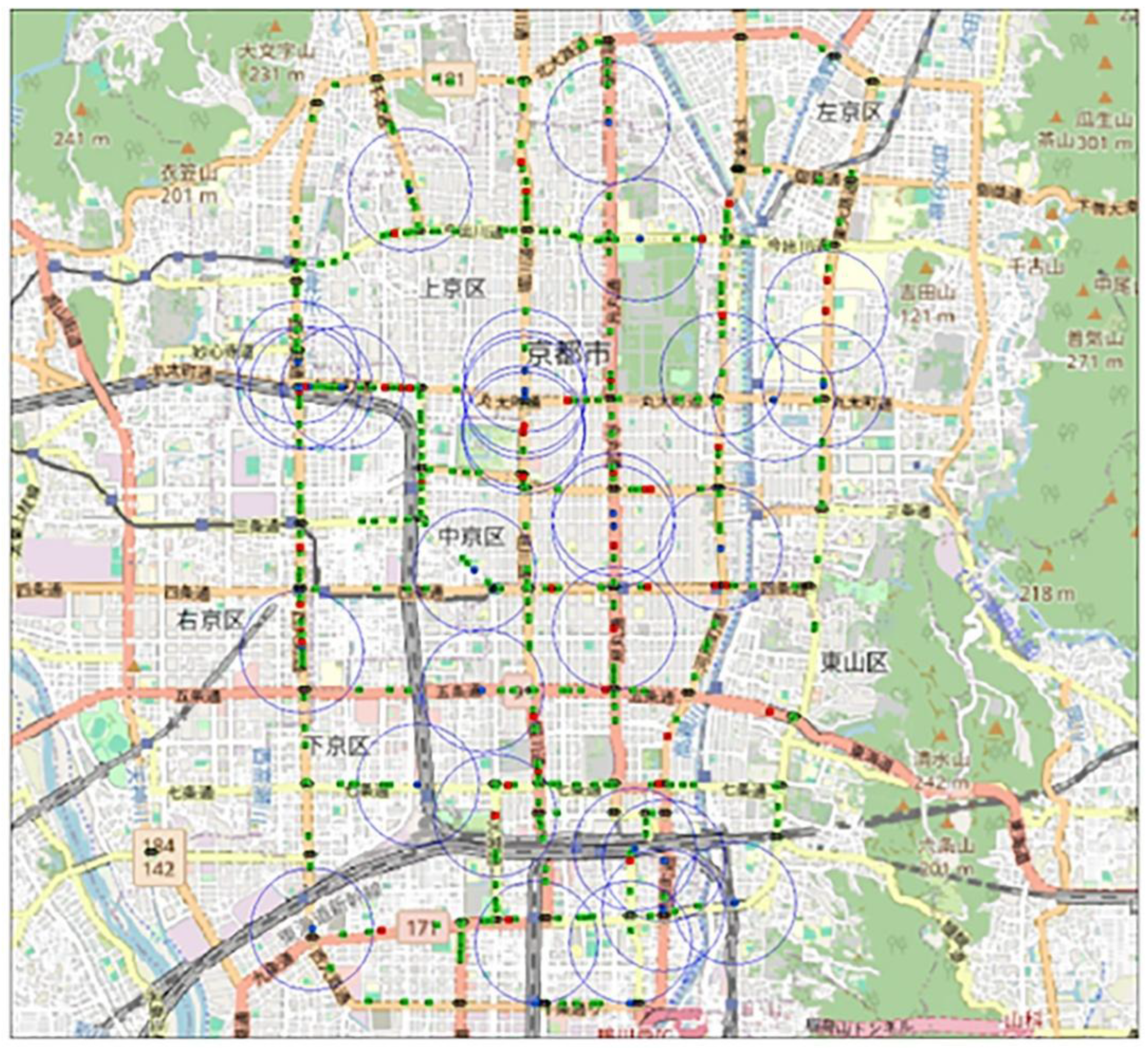
We conducted a simulation using Kyoto City as an example of a real city. The simulation used artisoc, a platform for multi-agent simulation developed by [27]. The screen used in the simulation is shown in Figure 4. Vehicle agents were colour-coded to distinguish between conventional vehicles and CAVs, as well as to indicate low-speed driving conditions. The communication range of each CAV is indicated by a blue circle.
Figure 4.
Visual output of the simulation.
In the simulation, we used a road network extracted from national highways (trunk), major prefectural roads (primary), and general prefectural roads (secondary) in Kyoto (Figure 5). The road network in Kyoto comprises 112 points (nodes) and 152 roads (links).
The parameters associated with the driving behaviours of vehicle agents were set as follows: maximum speed vmax = 1, acceleration a = 0.334, and minimum safe distance dmin = 1. In addition, because the maximum standard travel time was 248, data collection was initiated after 250 steps and ended when 3,000 vehicles reached their destinations. Although a larger number of vehicles reaching their destinations would improve the stability of the simulation results, the number was set to 3,000 considering the trade-off with computation time.
In the simulation, the communication range of the CAVs was varied in increments of 10 from a radius of 10 to 100, and the penetration rate of the CAVs (generation ratio) was varied in increments of 5% from 0% to 100%. A penetration rate of 0% represents a scenario in which the vehicle agents are conventional cars, whereas a penetration rate of 100% corresponds to a scenario in which all agents are connected.
The generation probability of vehicle agents is determined by the population assigned to each road endpoint (node). It is assumed that the higher the population assigned to a node, the higher the corresponding departure frequency. The population assigned to each node was based on the “500-meter Mesh Estimated Future Population Data (FY2018 National Government Office Estimate)” obtained from [28]. Figure 6 presents a colour-coded map indicating population density, with warmer colours representing areas with higher populations and cooler colours representing areas with lower populations. The population within each mesh block was allocated to the nodes contained within that block, and the population assigned to each node was proportionally determined based on the number of nodes in the mesh.
The probability of generating a vehicle agent with point (node) i as its origin is given by:
where δ is a parameter used to adjust the overall traffic volume in the simulation. In the simulation for Kyoto City, considering the numbers of nodes and generated agents, δ was set to 0.25.
Similarly, the destinations of the generated vehicle agents were determined probabilistically based on the population. The traffic demand between nodes was determined by the following gravity model, which is based on the population Pi of origin node i, population Pj of destination node j, and the straight-line (Euclidean) distance Lij between the nodes.
Here, σ1, σ2, and σ3 represent parameters of the gravity model, set as σ1 = 0.5393192, σ2 = 0.3702117, and σ3 = 1.666391, based on estimates from data on Japan’s three major metropolitan areas as reported by [29].
The probability that a vehicle agent generated at the origin node i will have node j as its destination is given by the following equation:
3.2. Results
Table 3 lists the CO₂ reduction rates, calculated using the average values from five experiments conducted for each parameter, with the CO₂ emissions at a CAV penetration rate of 0 used as the benchmark. In Table 3, a colour scale from red to blue is applied based on the CO₂ reduction rate. Additionally, the values for the highest CO₂ reduction, observed at a penetration rate of 1.0 and communication range of 75, are highlighted in bold white text. The results indicate that as the CAV penetration rate increases, CO₂ emissions decrease. Moreover, when the communication range is narrow, the benefits of CAVs are difficult to realise, even with a high penetration rate. For example, when the communication range is 5, the CO₂ reduction effect is at most just over 10%. A communication range of at least 30 is required to achieve a CO₂ reduction effect of more than 20%. However, the maximum communication range does not necessarily result in the highest CO₂ reduction effect.
In addition, curve fitting to the logistic growth model was performed after applying Min–Max scaling to the total CO₂ emissions y using the minimum value ymin and maximum value ymax from the experimental data. The logistic growth model was originally developed to describe natural population growth and has since been applied to various phenomena, such as product diffusion and the spread of infectious diseases. The independent variable in the logistic growth model typically represents time, or more generally, the progression or phase of growth. Given the theoretical background and nature of the model, the logistic growth model was adopted in this study. The scaled total CO2 emissions yscaled can be estimated as a function of the CAV penetration rate x using the following equation:
where K represents the maximum CO₂ emissions (upper bound), β is a coefficient that controls the slope (strength of the CO₂ reduction effect), and x0 denotes the inflection point (penetration rate at which CO₂ reduction is most effective). Because yscaled is scaled using the maximum CO₂ emissions ymax, K is fixed at 1.
The results of the curve fitting to the logistic growth model are presented in Table 4. For all communication ranges of CAVs, the coefficient of determination R2 exceeded 0.9, indicating an excellent fit. The strong fit to the logistic model illustrates that the CO₂ reduction effect is relatively small at low CAV penetration rates, increases rapidly as the penetration rate approaches the inflection point x0, and eventually saturates as x approaches 100%. However, the strength of the CO₂ reduction effect β and the location of the inflection point x0 vary depending on the communication range of the CAVs.
When plotting the relationship between the scaled total CO₂ emissions and CAV penetration rate, the logistic curve takes a gently inverted S-shape when β < 0 and |β| is small (Figure 7(a)) and a steeply inverted S-shape when β < 0 and |β| is large (Figure 7(b)). In this study, once the communication range exceeded approximately 25, |β| reached approximately 5.0, and the logistic function takes on a clearly inverted S-shape, indicating that beyond a certain penetration rate, the CO₂ reduction effect emerges explosively. Furthermore, the inflection point x0 was generally observed between 0.5 and 0.6, meaning that when the CAV penetration rate reached approximately 50–60%, a sharp decrease in CO₂ emissions occurred. However, when the communication range is narrow (e.g., 20 or below), the penetration rate must be considerably higher before any meaningful CO₂ reduction can be achieved.
Next, we examined the relationship between the CAV communication range and the strength of the CO2 reduction effect. As shown in the table within Figure 8, the strength of the CO2 reduction effect when CAVs are widely adopted varies depending on their communication ranges. In the communication range of 5 to 65, the strength of the CO2 reduction effect shows a decreasing trend. In contrast, from 65 to 100, the strength increases. When the communication range is narrow, a CAV may struggle to find other CAVs to share information, thereby limiting its functionality.
Moreover, the relationship between the communication range r of CAVs and the strength of the CO2 reduction effect β can be approximated by a quadratic equation (as shown in the graph in Figure 8). This finding indicates that if the information-sharing range is too wide, the CO2 reduction effect decreases. As the information-sharing range expands, the differences in the information obtained by each CAV diminish, causing them to select the same route. Consequently, traffic congestion occurs not only on the shortest routes but also on specific alternate roads. Vehicles that avoid congestion by choosing detour routes based on traffic information may contribute to congestion on those roads, resulting in an unintended increase in CO2 emissions. This paradoxical outcome suggests that the current centralised car navigation systems, which collect road traffic information and uniformly distribute the same data to all vehicles, may be inefficient. In contrast, local information sharing can prevent excessive concentration on detour routes and improve traffic distribution. In other words, by appropriately limiting the communication range and allowing CAVs to make self-interested route choices based on local information, traffic can be naturally dispersed through swarm intelligence, without the need for cooperative control.
4. Conclusions
In this study, we examined the effect of CO2 emission reduction through the exchange of road information between vehicles using a multi-agent simulation. Because the reduction in CO2 emissions was limited when the penetration rate of CAVs was low, the proactive promotion of CAV adoption was particularly important in the early stages. However, when the penetration rate was low, the reduction effect on CO₂ emissions remained minimal; thus, actively promoting CAV adoption in the early stages to achieve significant benefits was essential. In particular, when the communication range of CAVs was narrow, a high penetration rate was required before any noticeable reduction in CO₂ emissions could be achieved. Meanwhile, a wider communication range did not necessarily lead to greater CO₂ reduction. In fact, when the communication range became excessively large, the reduction effect weakened. In this study, non-cooperative control of CAVs was implemented, and route choice was entirely left to individual CAVs. Even if each CAV behaved selfishly, CO₂ emissions could still be reduced through information sharing among vehicles. Therefore, by adjusting the range of shared information, it may be possible to alleviate traffic congestion and reduce CO2 emissions without falling into this paradox, thereby maximising the use of road traffic information. However, since the present simulation is based on a simplified model, the CO₂ reduction effect may have been overestimated. For a more detailed analysis, it is necessary to conduct verification using a real-world framework such as COPERT, which is the standard tool for calculating carbon dioxide emissions in the EU. In future research, the optimal communication range for information sharing will require a network of CAVs. However, the exchange of information between CAVs in the network can lead to traffic paradoxes, making it necessary to limit the network distance over which information can be shared.
Author Contributions
Conceptualization, H.I., T.H. and Y.K.; methodology, H.I. and Y.K.; software, H.I.; validation, H.I., T.H. and Y.K.; formal analysis, H.I. and Y.K.; investigation, T.H.; resources, H.I.; data curation, H.I.; writing—original draft preparation, H.I.; writing—review and editing, T.H. and Y.K.; visualization, H.I.; supervision, Y.K.; project administration, T.H.; funding acquisition, T.H. All authors have read and agreed to the published version of the manuscript.
Funding
This study was supported by JSPS KAKENHI Grant Number JP21K01515.
Data Availability Statement
Additional data will be made available based on request.
Acknowledgments
During the preparation of this paper, the author used Python 3.11 for analyzing the simulation results and QGIS 3.30.0 for handling geospatial data. The authors gratefully acknowledge KOZO KEIKAKU ENGINEERING Inc. for providing artisoc, the multi-agent simulation platform used in this research. The authors have reviewed and edited the output and take full responsibility for the content of this publication.
Conflicts of Interest
The authors declare no conflicts of interest. The funders had no role in the design of the study; in the collection, analyses, or interpretation of data; in the writing of the manuscript; or in the decision to publish the results.
Abbreviations
The following abbreviations are used in this manuscript:
| AI | Artificial Intelligence |
| CAV(s) | Connected Autonomous Vehicle(s) |
| DOAJ | Directory of Open Access Journals |
| DSRC | Dedicated Short Range Communication |
| GHG | Greenhouse Gas |
| ITS | Intelligent Transportation Systems |
| LD | Linear Dichroism |
| LED | Light Emitting Diode |
| LTE | Long Term Evolution |
| MAS | Multi-Agent Simulation |
| MDPI | Multidisciplinary Digital Publishing Institute |
| TLA | Three-Letter Acronym |
| V2V | Vehicle-to-Vehicle |
| VoT | Value of Time |
References
- Shi, X.; Yao, H.; Liang, Z.; Li, X. An empirical study on fuel consumption of commercial automated vehicles. Transp. Res. Part D Transp. Environ. 2022, 106, 103253. [Google Scholar] [CrossRef]
- Ma, F.; Yang, Y.; Wang, J.; Li, X.; Wu, G.; Zhao, Y.; Wu, L.; Aksun-Guvenc, B.; Guvenc, L. Eco-driving-based cooperative adaptive cruise control of connected vehicles platoon at signalized intersections. Transp. Res. Part D Transp. Environ. 2021, 92, 102746. [Google Scholar] [CrossRef]
- Shen, M.; He, C.R.; Molnar, T.G.; Bell, A.H.; Orosz, G. Energy-efficient connected cruise control with lean penetration of connected vehicles. IEEE Trans. Intell. Transp. Syst. 2023, 24, 4320–4332. [Google Scholar] [CrossRef]
- Djavadian, S.; Tu, R.; Farooq, B.; Hatzopoulou, M. Multi-objective eco-routing for dynamic control of connected and automated vehicles. Transp. Res. Part D Transp. Environ. 2020, 87, 102513. [Google Scholar] [CrossRef]
- Pribyl, O.; Blokpoel, R.; Matowicki, M. Addressing EU climate targets: Reducing CO₂ emissions using cooperative and automated vehicles. Transp. Res. Part D Transp. Environ. 2020, 86, 102437. [Google Scholar] [CrossRef]
- Braess, D. Über ein Paradoxon aus der Verkehrsplanung. Unternehmensforsch.–Oper. Res.–Rech. Opér. 1968, 12, 258–268. [Google Scholar] [CrossRef]
- Braess, D.; Nagurney, A.; Wakolbinger, T. On a paradox of traffic planning. Transp. Sci. 2005, 39, 446–450. [Google Scholar] [CrossRef]
- Asian Development Bank. Reducing Carbon Emissions from Transport Projects (Evaluation Study No. EKB: REG 2010-16); Asian Development Bank: Manila, Philippines, 2010. [Google Scholar]
- Youn, H.; Gastner, M.T.; Jeong, H. Price of anarchy in transportation networks: Efficiency and optimality control. Phys. Rev. Lett. 2008, 101. [Google Scholar] [CrossRef] [PubMed]
- Tu, R.; Alfaseeh, L.; Djavadian, S.; Farooq, B.; Hatzopoulou, M. Quantifying the impacts of dynamic control in connected and automated vehicles on greenhouse gas emissions and urban NO₂ concentrations. Transp. Res. Part D Transp. Environ. 2019, 73, 142–151. [Google Scholar] [CrossRef]
- Shimizu, H.; Matsubayashi, T.; Naya, F. Simulation of saturated theme park for reduction of waiting time. Trans. Jpn. Soc. Artif. Intell. (In Japanese). 2017, 32, AG16-F. [Google Scholar] [CrossRef]
- Vahidi, A.; Sciarretta, A. Energy saving potentials of connected and automated vehicles. Transp. Res. Part C Emerg. Technol. 2018, 95, 822–843. [Google Scholar] [CrossRef]
- Li, Y.; Shan, C. Impacts of cooperative adaptive cruise control links on driving comfort under vehicle-to-vehicle communication. J. Adv. Transp. 2022, 2022, 7248854. [Google Scholar] [CrossRef]
- Li, F.; Wang, Y. Routing in vehicular ad hoc networks: A survey. IEEE Veh. Technol. Mag. 2007, 2, 12–22. [Google Scholar] [CrossRef]
- Boskovich, S.; Boriboonsomsin, K.; Barth, M. A developmental framework towards dynamic incident rerouting using vehicle-to-vehicle communication and multi-agent systems. In Proceedings of the 13th International IEEE Conference on Intelligent Transportation Systems, Funchal, Portugal, 19–22 September 2010; pp. 789–794. [Google Scholar] [CrossRef]
- Bintoro, K.B.Y.; Permana, S.D.H.; Syahputra, A.; Arifitama, B. V2V communication in smart traffic systems: Current status, challenges and future perspectives. J. Processor 2024, 19, 21–31. [Google Scholar] [CrossRef]
- Yang, X.; Recker, W.W. Modelling dynamic vehicle navigation in a self-organizing, peer-to-peer, distributed traffic information system. J. Intell. Transp. Syst. 2006, 10, 185–204. [Google Scholar] [CrossRef]
- Wang, R.; Xu, Z.; Zhao, X.; Hu, J. V2V-based method for the detection of road traffic congestion. IET Intell. Transp. Syst. 2019, 13, 880–885. [Google Scholar] [CrossRef]
- Lu, M.; Taiebat, M.; Xu, M.; Hsu, S.C. Multiagent spatial simulation of autonomous taxis for urban commute: Travel economics and environmental impacts. J. Urban Plan. Dev. 2018, 144. [Google Scholar] [CrossRef]
- Xu, Z.; Zheng, Z.; Xiao, D.; Tu, R.; Ma, W.; Zheng, N. Assessing the impact of passenger compliance behaviour in CAVs on environmental benefits. Transp. Res. Part D Transp. Environ. 2024, 133, 104278. [Google Scholar] [CrossRef]
- Suzuki, T.; Matsuda, K.; Kumagae, K.; Tobisawa, M.; Hoshino, J.; Itoh, Y.; Harada, T.; Matsuoka, J.; Kagawa, T.; Hattori, K. Acquisition of cooperative control of multiple vehicles through reinforcement learning utilizing vehicle-to-vehicle communication and map information. J. Robot. Mechatron. 2024, 36, 642–657. [Google Scholar] [CrossRef]
- Takai, I.; Harada, T.; Andoh, M.; Yasutomi, K.; Kagawa, K.; Kawahito, S. Optical vehicle-to-vehicle communication system using LED transmitter and camera receiver. IEEE Photon. J. 2014, 6, 1–14. [Google Scholar] [CrossRef]
- Matolak, D.W. Channel modelling for vehicle-to-vehicle communications. IEEE Commun. Mag. 2008, 46, 76–83. [Google Scholar] [CrossRef]
- Lianghai, J.; Liu, M.; Weinand, A.; Schotten, H.D. Direct vehicle-to-vehicle communication with infrastructure assistance in 5G network. In Proceedings of the 16th Annual Mediterranean Ad Hoc Networking Workshop (Med-Hoc-Net), Budva, Montenegro, 28–30 June 2017; pp. 1–5. [Google Scholar] [CrossRef]
- Dey, K.C.; Rayamajhi, A.; Chowdhury, M.; Bhavsar, P.; Martin, J. Vehicle-to-vehicle (V2V) and vehicle-to-infrastructure (V2I) communication in a heterogeneous wireless network: Performance evaluation. Transp. Res. Part C Emerg. Technol. 2016, 68, 168–184. [Google Scholar] [CrossRef]
- Barth, M.; Boriboonsomsin, K. Real-world CO₂ impacts of traffic congestion. Transp. Res. Rec. 2008, 2058, 163–171. [Google Scholar] [CrossRef]
- KOZO KEIKAKU ENGINEERING Inc. MAS Community. Available online: https://mas.kke.co.jp/en/ (accessed on 13 March 2025).
- Ministry of Land, Infrastructure, Transport and Tourism. National Land Numerical Information Download Site. Available online: https://nlftp.mlit.go.jp/ksj/index.html (accessed on 29 August 2024).
- Hiramatsu, T.; Inoue, H.; Kato, Y. Analysing the formation of urban orbital road networks with multi-agent simulation. J. Transp. Econ. Policy 2021, 55, 36–63. [Google Scholar]
Figure 1.
Estimated travel time for route selection.
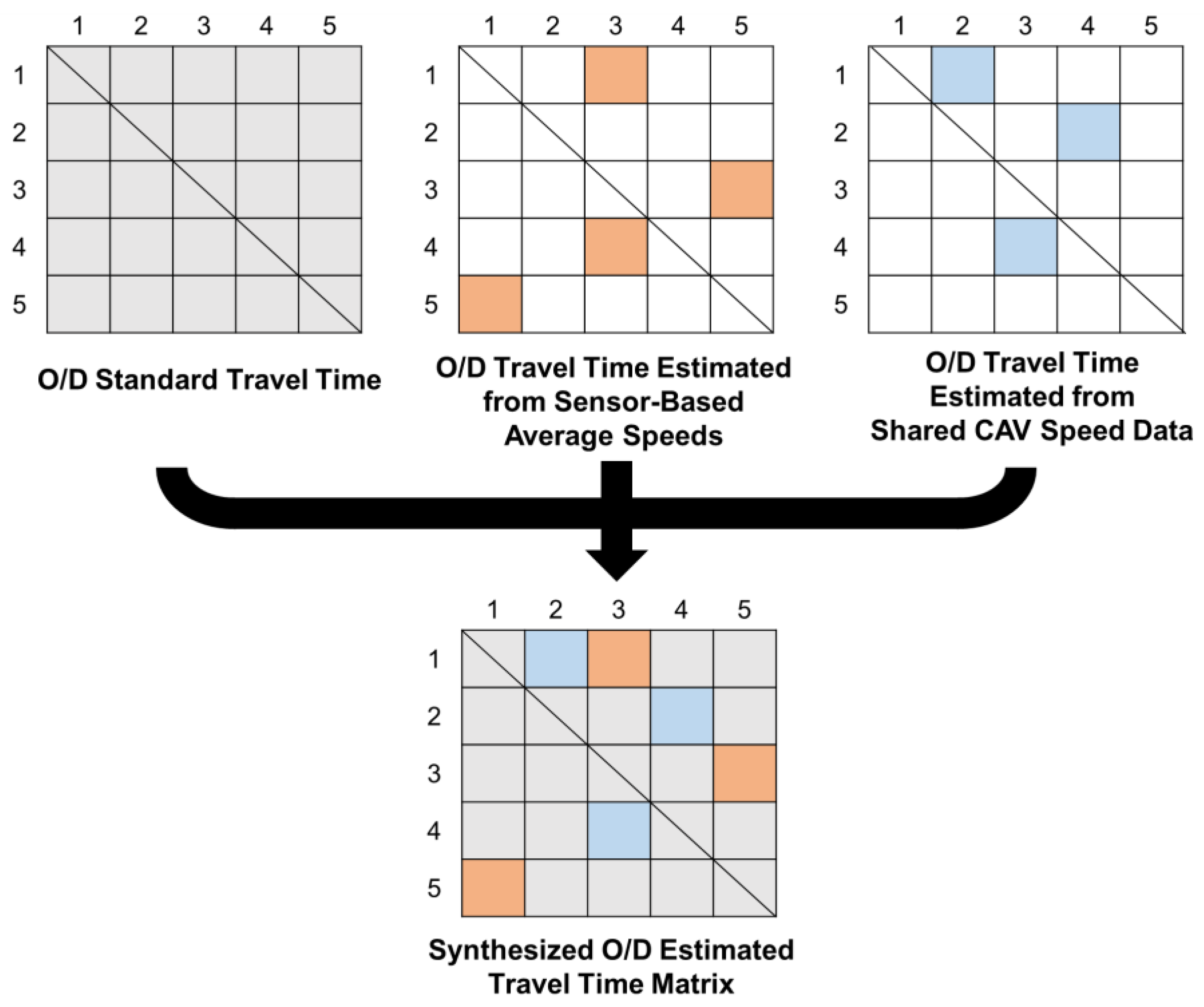
Figure 2.
Overview of car navigation system.
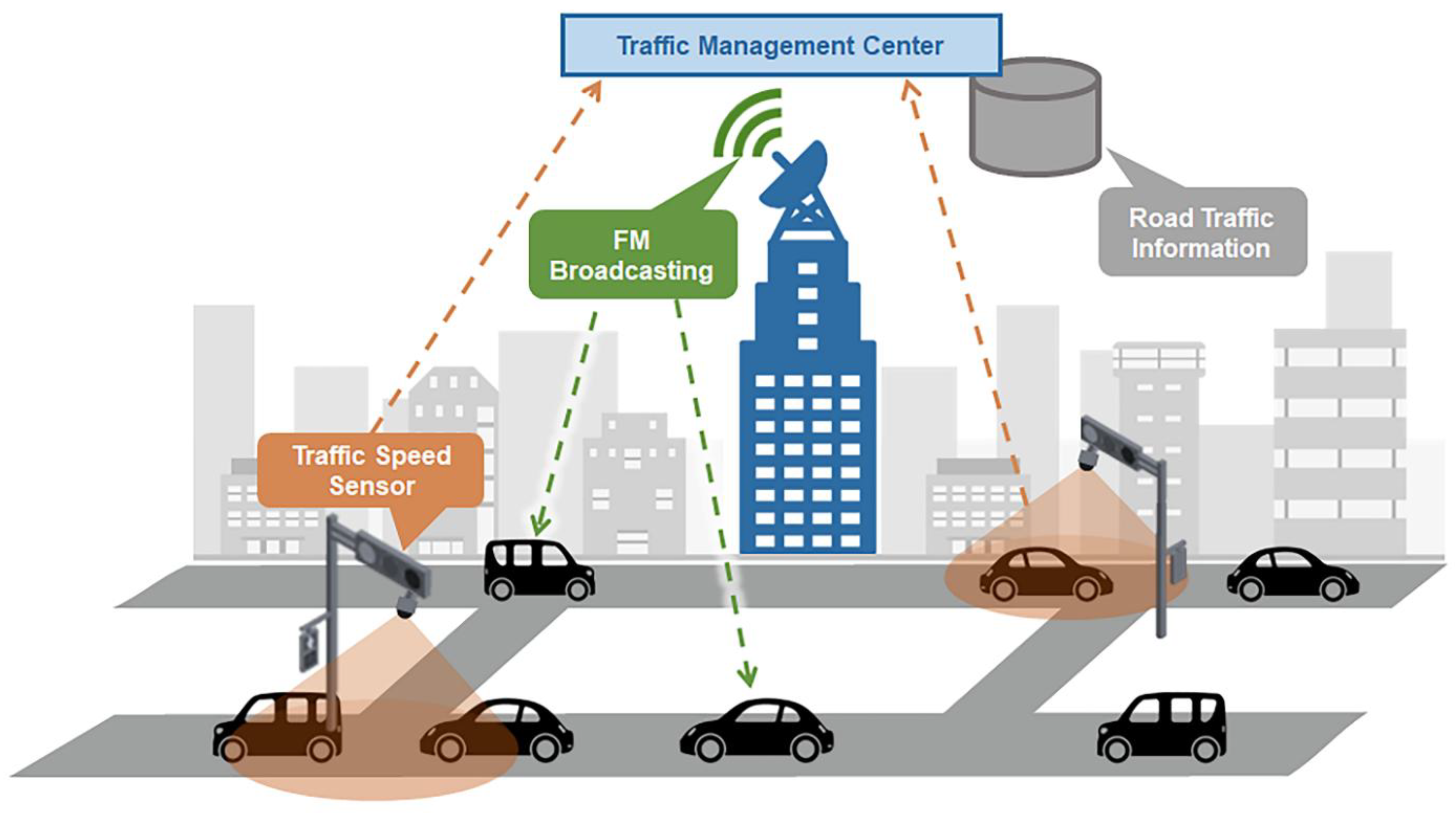
Figure 3.
Information sharing between CAVs.
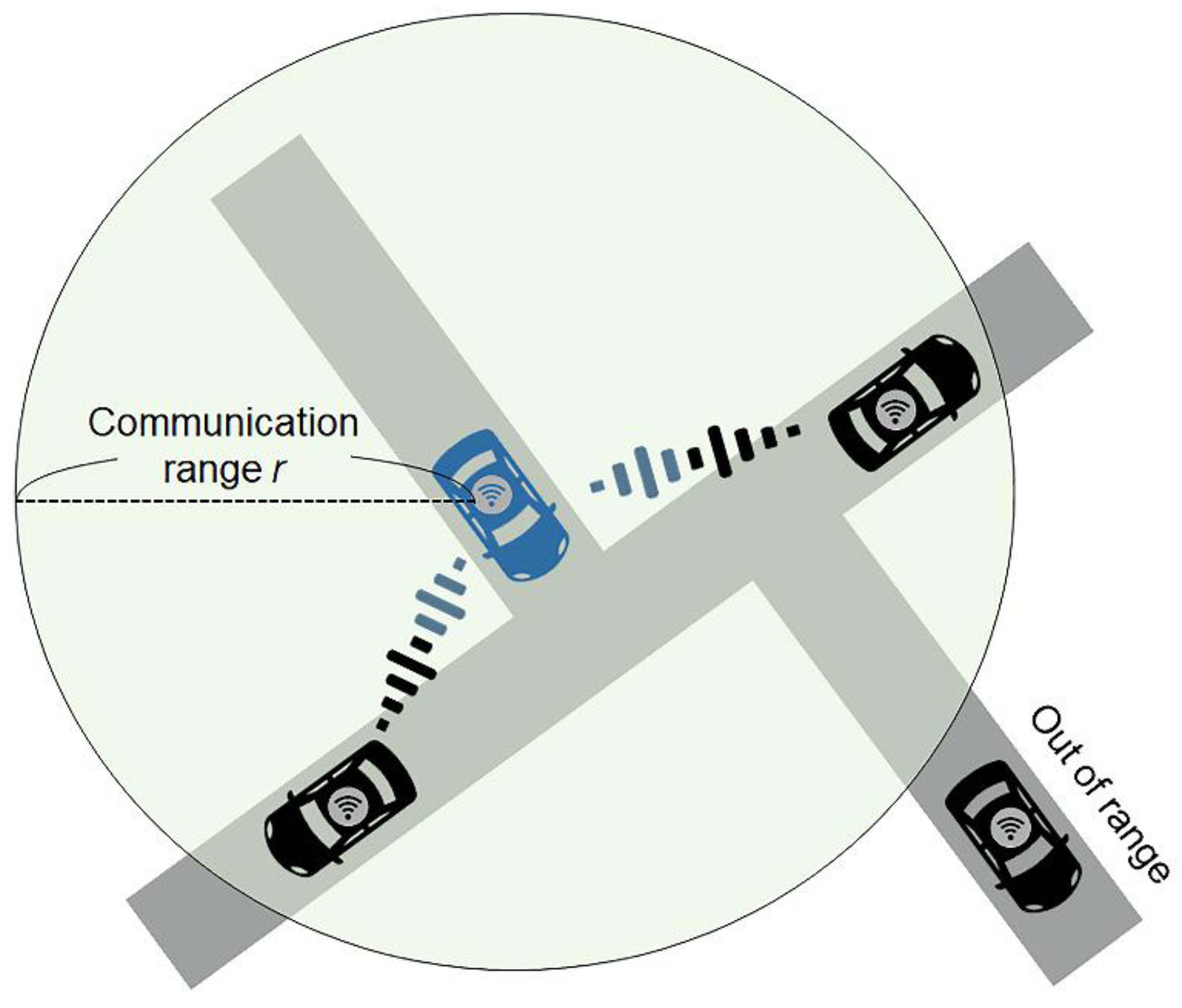
Figure 5.
Road network of Kyoto.
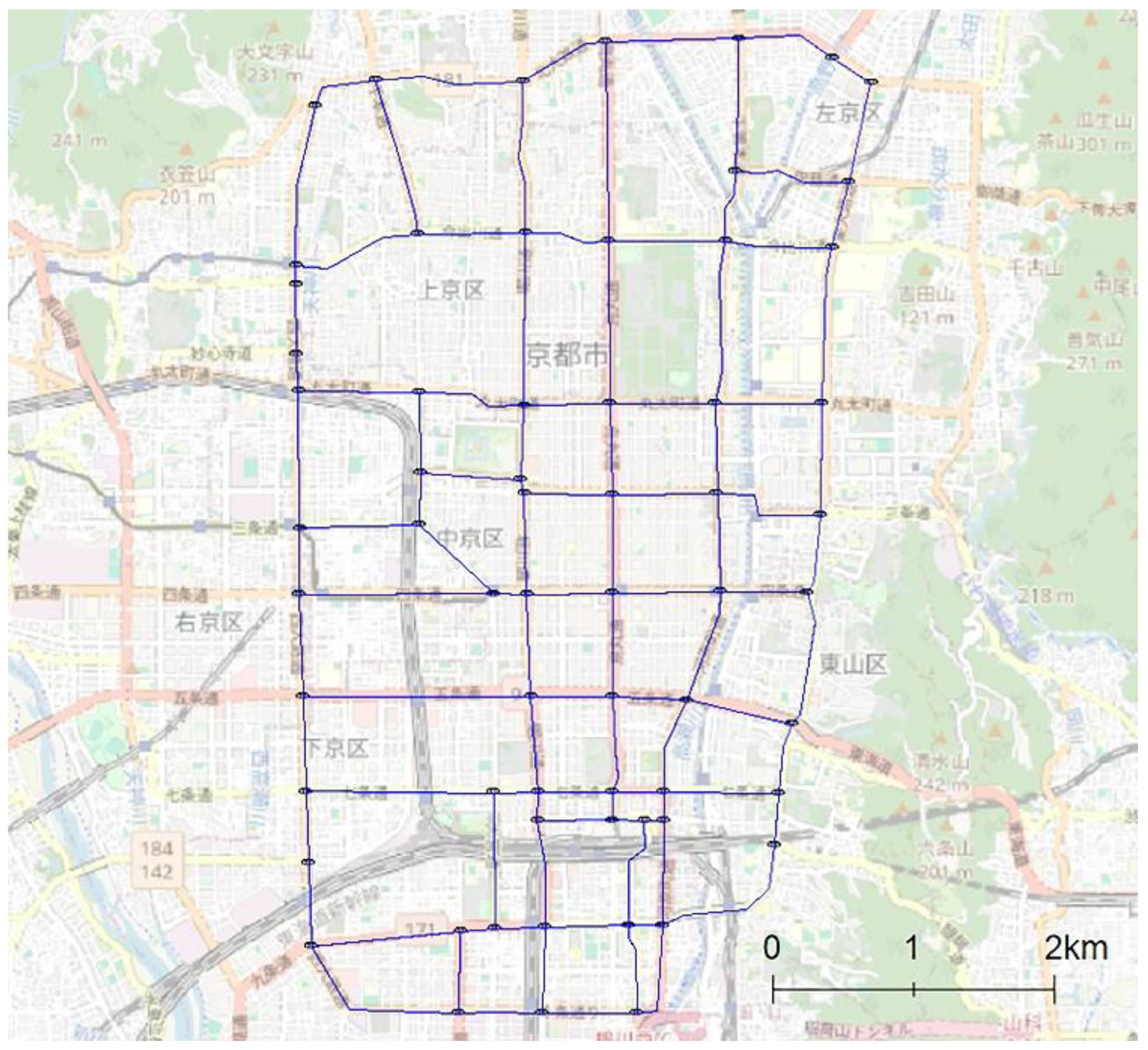
Figure 6.
500-meter mesh population.
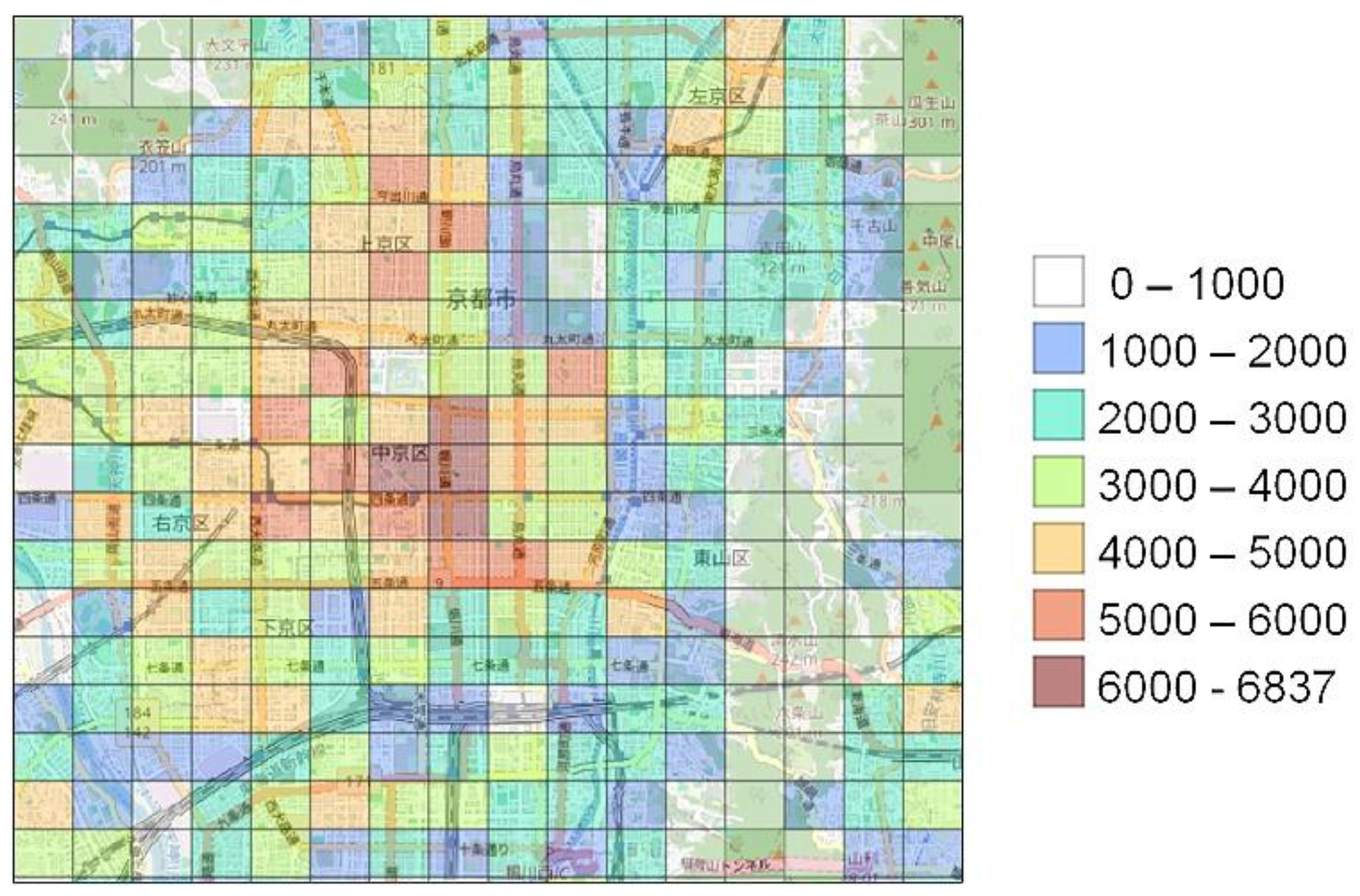
Figure 7.
Logistic curve fittings.
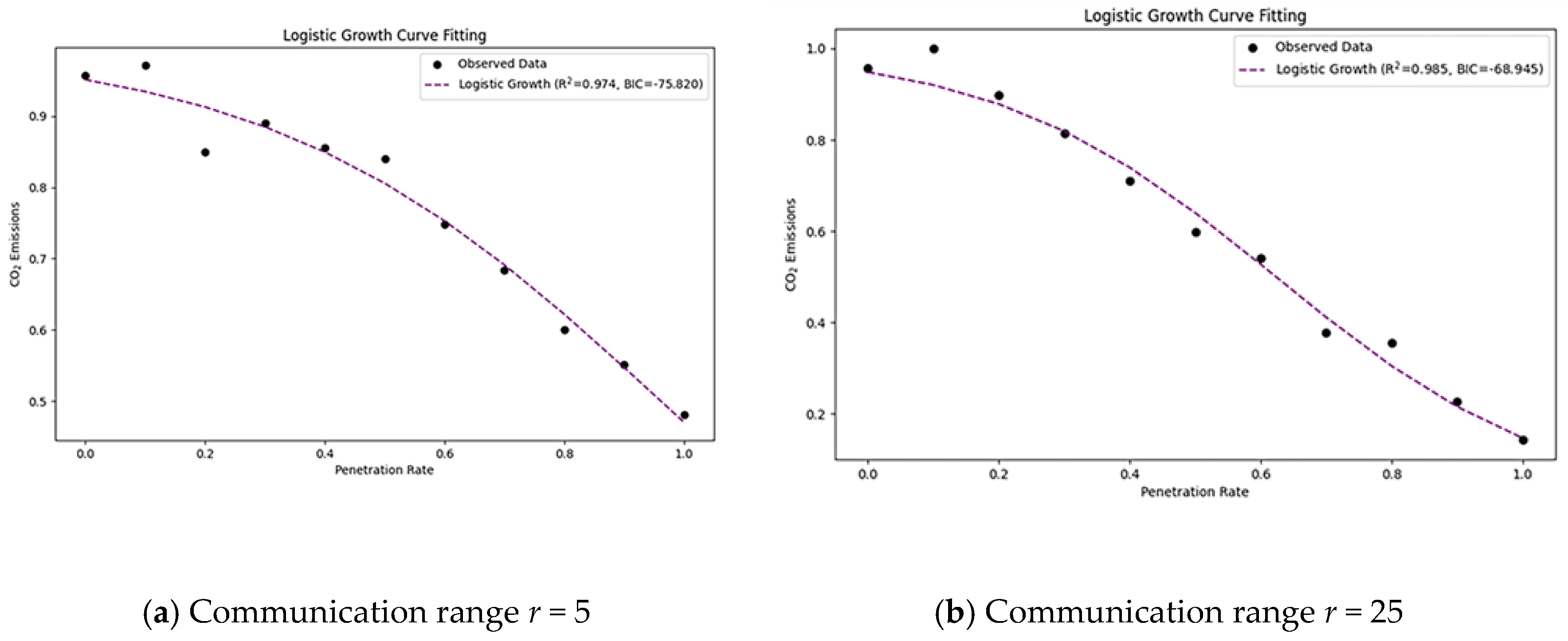
Figure 8.
CO2 reduction effect by communication range of CAVs.
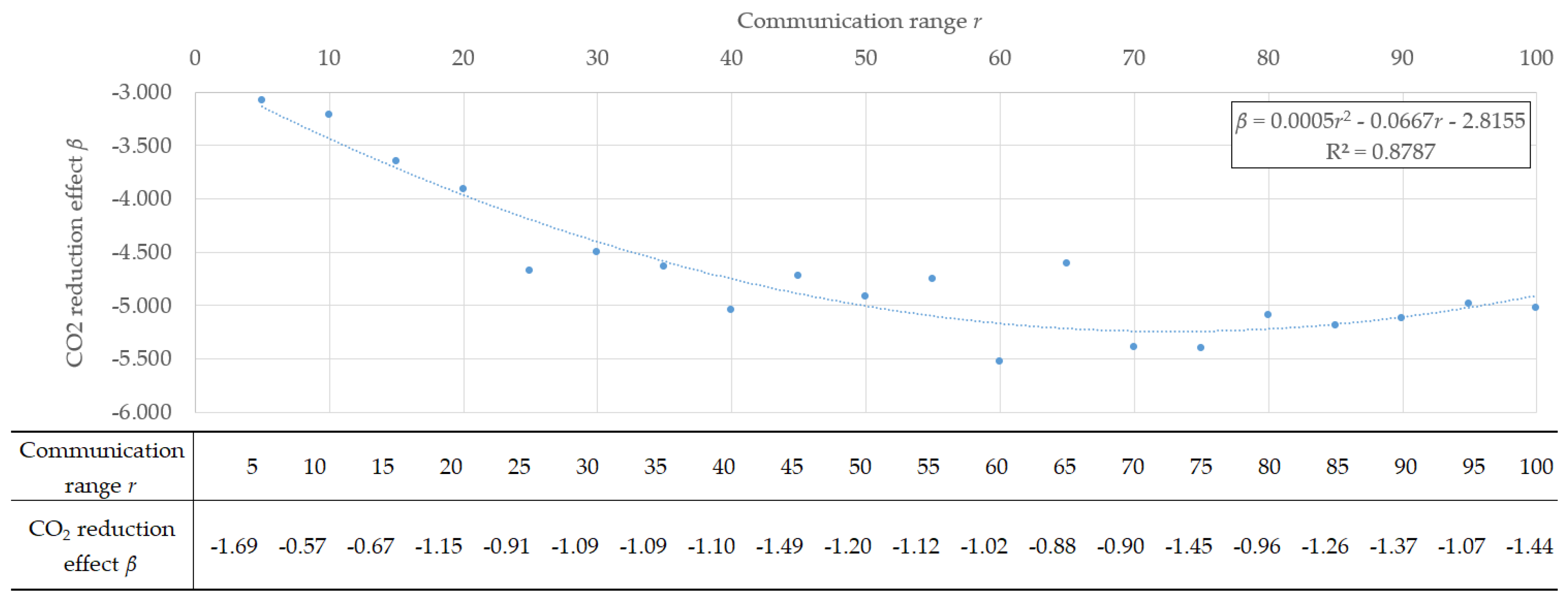

Table 1.
Availability of traffic information by car type.
| Car Type | Standard Travel Time | Traffic Speed Sensor Information | Shared Information Between CAVs |
|---|---|---|---|
| Conventional car | Y | Y | N |
| CAV | Y | Y | Y |
Table 2.
Parameters for estimating CO2 emissions.
| Parameter | Mph | kmph |
|---|---|---|
| b0 | 7.613534994965560 | 12.252766408797900 |
| b1 | -0.138565467462594 | -0.222998949406251 |
| b2 | 0.003915102063854 | 0.006300730355443 |
| b3 | -0.000049451361017 | -0.000079584053339 |
| b4 | 0.000000238630156 | 0.000000384037055 |
Source: Barth & Boriboonsomsin [26].
Table 3.
Experimental results.
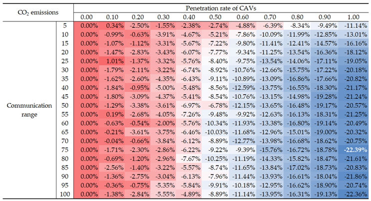
Table 4.
Estimated parameters of the logistic growth model.
| Communication range r | β | x0 | R2 |
|---|---|---|---|
| 5 | -3.083 | 0.962 | 0.974 |
| 10 | -3.214 | 0.781 | 0.965 |
| 15 | -3.653 | 0.690 | 0.985 |
| 20 | -3.909 | 0.649 | 0.994 |
| 25 | -4.675 | 0.623 | 0.985 |
| 30 | -4.505 | 0.593 | 0.991 |
| 35 | -4.640 | 0.573 | 0.992 |
| 40 | -5.041 | 0.567 | 0.987 |
| 45 | -4.729 | 0.583 | 0.984 |
| 50 | -4.917 | 0.572 | 0.986 |
| 55 | -4.758 | 0.581 | 0.979 |
| 60 | -5.528 | 0.573 | 0.986 |
| 65 | -4.608 | 0.571 | 0.982 |
| 70 | -5.390 | 0.567 | 0.992 |
| 75 | -5.401 | 0.568 | 0.978 |
| 80 | -5.095 | 0.562 | 0.982 |
| 85 | -5.189 | 0.573 | 0.992 |
| 90 | -5.126 | 0.576 | 0.990 |
| 95 | -4.987 | 0.578 | 0.981 |
| 100 | -5.022 | 0.564 | 0.980 |
Disclaimer/Publisher’s Note: The statements, opinions and data contained in all publications are solely those of the individual author(s) and contributor(s) and not of MDPI and/or the editor(s). MDPI and/or the editor(s) disclaim responsibility for any injury to people or property resulting from any ideas, methods, instructions or products referred to in the content. |
© 2025 by the authors. Licensee MDPI, Basel, Switzerland. This article is an open access article distributed under the terms and conditions of the Creative Commons Attribution (CC BY) license (http://creativecommons.org/licenses/by/4.0/).
Copyright: This open access article is published under a Creative Commons CC BY 4.0 license, which permit the free download, distribution, and reuse, provided that the author and preprint are cited in any reuse.


